Spatial Wilson loops in the classical field of high-energy heavy-ion collisions

Abstract

It has been previously shown numerically that the expectation value of the magnetic Wilson loop at the initial time of a heavy-ion collision exhibits area law scaling. This was obtained for a classical non-Abelian gauge field in the forward light cone and for loops of area $A\,\,\vbox{\hbox{$\buildrel\displaystyle>\over{\sim}$}}\,\,2/Q_{s}^{2}$. Here, we present an analytic calculation of the spatial Wilson loop in the classical field of a collision within perturbation theory. It corresponds to a diagram with two sources, for both projectile and target, whose field is evaluated at second order in the gauge potential. The leading non-trivial contribution to the magnetic loop in perturbation theory is proportional to the square of its area.

In high-energy collisions the target and the projectile are represented as Lorentz-contracted sheets of valence color charges moving along recoilless trajectories along the light cone. These charges act as sources of a purely transverse gluon field that has a small fraction $x$ of the total longitudinal momentum of the nucleus. Since the charge density $\rho(\bf x)$ is large, the sources belong to a higher dimensional representation of the color algebra and the gauge field they emit can be computed classically MV . After the two sheets of color charge have passed through each other, longitudinal chromo-electric and chromo-magnetic fields are produced Fries:2006pv_TL_LM_KKV . The fluctuations of the chromo-magnetic flux may be viewed as uncorrelated vortices with a typical radius $\sim 0.8/Q_{s}$ DNP . $Q_{s}$ denotes the saturation momentum which is the scale where the gluon field exhibits non-linear dynamics Saturation . The effective area law behavior of the magnetic flux which indicated vortex structure was obtained in ref. DNP numerically. Here we provide some analytic insight within perturbation theory and compare it to the lattice computation. Since the perturbative expansion of the magnetic flux applies only to small loops ($A\ll 1/Q_{s}^{2}$) it may of course deviate from the lattice result obtained for large loops. Indeed, the latter resums screening corrections to the magnetic field DumitruFujiiNara .

The gluon field of the target and the projectile is obtained by solving the classical Yang-Mills equations of motion. Before the collision, the solution corresponds to a non-Abelian analogue of the Weizsäcker-Williams field. In light-cone gauge its form is:

$$\alpha^{i}_{m}=\frac{i}{g}\,U_{m}\,\partial^{i}U_{m}^{\dagger}~{}~{}~{}~{},~{}~{}~{}~{}\partial^{i}\alpha^{i}_{m}=g\rho_{m}~{}.$$ (1)

The subscript $m$, with values 1 and 2, denotes the projectile and the target respectively. Introducing the gauge potential as

$$\Phi_{m}=-\frac{g}{\nabla_{\perp}^{2}}\rho_{m}~{},$$ (2)

the solution to (1) can be written as Kovner:1995ja :

$$\alpha_{m}^{i}=\frac{i}{g}e^{-ig\Phi_{m}}\partial^{i}e^{ig\Phi_{m}}~{}.$$ (3)

The Yang-Mills equations for scattering of two ultra-relativistic nuclei with appropriate boundary conditions on the light cone give the classical field after the collision Kovner:1995ja . At proper time $\tau=\sqrt{t^{2}-z^{2}}=0$, the resulting field is a sum of two pure gauge fields:

$$A^{i}=\alpha_{1}^{i}+\alpha_{2}^{i}~{}.$$ (4)

The sum of two pure gauges is not a pure gauge and strong longitudinal chromo-electric and chromo-magnetic fields are produced in the collision Fries:2006pv_TL_LM_KKV :

$$E_{z} = ig[\alpha_{1}^{i},\alpha_{2}^{i}]~{},$$

$$B_{z} = ig\epsilon^{ij}[\alpha_{1}^{i},\alpha_{2}^{j}]~{}~{}~{},~{}~{}~{}(i,j=1,2)~{}.$$ (5)

$\epsilon^{ij}$ is the antisymmetric tensor. The transverse components of the field strength are zero.

The non-Abelian Wilson loop operator is defined as a path order exponential of the gauge field:

$$M(R) = {\cal P}\exp\left(ig\oint dx^{i}A^{i}\right)$$ (6)

$$= {\cal P}\exp\left[ig\oint dx^{i}\left(\alpha_{1}^{i}+\alpha_{2}^{i}\right)\right]~{},$$

with $R$ the radius of the loop. Note that $M(R)\equiv 1\!\!1$ if evaluated in the field of a single nucleus ($\alpha_{1}^{i}$ or $\alpha_{2}^{i}$) as those are pure gauges. In DNP it was shown that the expectation value of the magnetic Wilson loop in the field $A^{i}$ produced in a collision of two nuclei is proportional to the exponent of the area $A$ of the loop:

$$W_{M}(R)=\frac{1}{N_{c}}\left<{\rm tr}\,M(R)\right>\sim\exp\left(-\sigma_{M}A\right)~{}.$$ (7)

Here, $\sigma_{M}$ is the magnetic string tension. For the SU(2) gauge group its value was estimated to be $\sigma_{M}\simeq 0.12Q_{s}^{2}$. The result (7) was obtained for areas $A\,\,\vbox{\hbox{$\buildrel\displaystyle>\over{\sim}$}}\,\,2/Q_{s}^{2}$. It indicates that the structure of the chromo-magnetic flux at such scales corresponds to uncorrelated vortex fluctuations.

The expectation value in (7) refers to averaging over the color charge distributions in each nucleus. For large nuclei the color sources are treated as random variables with Gaussian probability distribution. Physical observables are then averaged with a Gaussian (McLerran-Venugopalan) action:

$$S_{\rm eff}[\rho^{a}]=\frac{1}{2}\int d^{2}\bf{x}\left[\frac{\rho_{1}^{a}({\bf x})\rho_{1}^{a}({\bf x})}{\mu^{2}_{1}}+\frac{\rho_{2}^{a}({\bf x})\rho_{2}^{a}({\bf x})}{\mu^{2}_{2}}\right]~{},$$ (8)

where $\mu^{2}$ is the color charge squared per unit area, related to the saturation scale via $Q_{s}^{2}\sim g^{4}\mu^{2}$.

To obtain $W_{M}(R)$ we need to determine the deviation of $A^{i}$ from a pure gauge. From the Baker-Campbell-Hausdorff formula DNP

$$W_{M}(R)\simeq\frac{1}{N_{c}}\left<{\rm tr}\,\exp\left(-\frac{1}{2}\left[X_{1},X_{2}\right]\right)\right>\simeq 1-\frac{1}{2N_{c}}\left<g^{2}h^{2}\right>~{},$$ (9)

where:

$$g^{2}h^{2}=\frac{1}{8}f^{abc}f^{\bar{a}\bar{b}c}X_{1}^{a}X_{1}^{\bar{a}}X_{2}^{b}X_{2}^{\bar{b}}~{}.$$ (10)

with:

$$X_{m}=ig\oint dx^{i}\alpha_{m}^{ai}t^{a}~{}.$$ (11)

$f^{abc}$ are the structure constants of the special unitary group and $h^{2}$ corresponds to a four gluon vertex of the fields.

To calculate this expectation value analytically, we expand the fields $\alpha^{i}$ from eq. (3) perturbatively in terms of the coupling constant:

$$\alpha_{m}^{i}= - \partial^{i}\Phi_{m}+\frac{ig}{2}\left(\delta^{ij}-\partial^{i}\frac{1}{\nabla_{\perp}^{2}}\partial^{j}\right)\left[\Phi_{m},\partial^{j}\Phi_{m}\right]$$ (12)

$$+ \mathcal{O}\left(\Phi_{m}^{3}\right)~{}.$$

The loop integral over the first term in (12) vanishes. Therefore, the leading term in the expansion of the field $\alpha^{i}$ in terms of the gauge potential $\Phi$ does not contribute to the Wilson loop $W_{M}$ and it is required to go to quadratic order: $\alpha^{i,a}\sim gf^{abc}\Phi^{b}\partial^{i}\Phi^{c}$:

$$X_{m}=-\frac{g^{2}}{2}\oint dx^{i}~{}\left[\Phi_{m},\partial^{i}\Phi_{m}\right]~{}.$$ (13)

The Feynman diagram representation of the expansion of the field $\alpha^{i}$ is given in fig. 1. At this order the field is still dominated by classical diagrams Kovchegov .

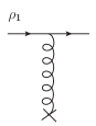
(a)

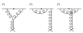
(b)

Figure 1: Diagram representation of the classical gauge field of a single nucleus to first (1a) and second order (1b) Kovchegov .

The expectation value $\left<h^{2}\right>$ that enters in the expression for the magnetic loop involves the fields of both nuclei. The corresponding classical diagram is shown in fig. 2a. A quantum correction at the same order is given in fig. 2b. We defer an analysis of quantum corrections to future work since the primary goal of this paper is to provide a point of comparison to resummed classical lattice gauge computations of the loop DNP which consider strong fields. However, our present analysis should not be taken to imply that small loops in weak fields can be obtained in the classical approximation.

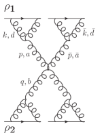
(a)

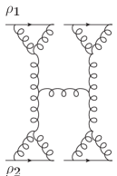
(b)

Figure 2: Classical (2a) and quantum (2b) contributions to the expectation value of the Wilson loop.

The final result we obtain for the expectation value of the magnetic Wilson loop for classical fields $\alpha^{i}$ to second order in the gauge potential is:

$$W_{M}(R)\simeq 1-\frac{\pi^{2}N_{c}^{6}}{64(N_{c}^{2}-1)^{3}}\frac{Q_{s1}^{4}Q_{s2}^{4}}{\Lambda^{4}}A^{2}~{}.$$ (14)

Details of the calculation are given in the appendix. $Q_{s1}$ and $Q_{s2}$ are the saturation scales of the projectile and the target, respectively. They are determined by the variance of the color charge distribution. We use the relation:

$$Q_{s}^{2}=\frac{g^{4}C_{F}}{2\pi}\mu^{2}~{},$$ (15)

where:

$$C_{F}=\frac{N_{c}^{2}-1}{2N_{c}}~{}.$$ (16)

The cut-off $\Lambda$ regulates the infrared divergence of the integrals over the gluon momentum $k$ shown in diagram 2a. It sets the mass scale for the gluon propagator.

From a fit to the lattice data for the Wilson loop for small areas, it was estimated that $W_{M}(R)\simeq 1-2\left(AQ_{s}^{2}\right)^{2}$ DNP . By comparing this expression to the result (14) for $SU(2)$ we can extract $Q_{s}^{4}/\Lambda^{4}\approx 5.477$.

We have calculated the expectation value of the magnetic loop with a Gaussian action. For a finite nuclear thickness, higher order corrections in the charge density of cubic JeonVenugopalan and quartic DJP order arise. As shown in the appendix, the calculation consists of averaging four-point functions and therefore the cubic part of the effective action does not contribute. On the other hand, one would expect the fourth order term to bring a correction to the four-point function. However, the correction to the Wilson loop from the quartic action vanishes because of its vanishing color factor (see appendix).

We now turn to a discussion of the final result (14). The perturbative result for the expectation value of the magnetic Wilson loop gives a leading non-trivial contribution that is proportional to the square of the area. A term proportional to the area of the loop would involve single powers of the target’s and projectile’s saturation scales: $\sim A~{}Q_{s1}Q_{s2}$ DNP . However, Gaussian contractions can only give powers of $Q_{s1}^{2}$ and $Q_{s2}^{2}$:

$$\langle\rho^{a}_{m}({\bf x})\,\rho^{b}_{m}({\bf y})\rangle=\mu_{m}^{2}\delta^{ab}\delta({\bf x}-{\bf y})\sim Q_{s_{m}}^{2}~{},$$ (17)

and therefore a contribution $\sim A^{2}$. Area law scaling of the Wilson loop presumably requires resummation of screening effects and of condensation.

I Appendix

In the appendix we list some steps of the calculation leading to the final result (14). To calculate the expectation value of the Wilson loop, we need the average:

$$\left<g^{2}h^{2}\right>=\frac{1}{8}f^{abc}f^{\bar{a}\bar{b}c}\left<X_{1}^{a}X_{1}^{\bar{a}}\right>_{\rho_{1}}\left<X_{2}^{b}X_{2}^{\bar{b}}\right>_{\rho_{2}}~{}.$$ (18)

Using the second term in the expression for the fields $\alpha_{m}$ in eq. (12) we have:

$$X_{m}^{a}=-\frac{ig^{2}}{2}f^{ade}\oint dx^{i}~{}\Phi_{m}^{d}\partial^{i}\Phi_{m}^{e}~{},$$ (19)

or, in momentum space:

$$X_{m}^{a}=-\frac{ig^{2}}{2(2\pi)^{3}}f^{ade}R\times$$

$$\int d^{2}{\bf k}d^{2}{\bf p}|{\bf k}|J_{1}(R|{\bf p}|)~{}\sin(\alpha-\theta)\Phi_{m}^{d}({\bf k})\Phi_{m}^{e}({\bf p}-{\bf k})~{}.~{}~{}~{}$$ (20)

In the above expression, $R$ is the radius of the loop, $k$ and $p$ are the momenta of the gluons shown in fig. 2a, and $\alpha$ and $\theta$ are their corresponding azimuthal angles. $J_{1}(R|{\bf p}|)$ is a Bessel function of the first kind. Then:

$$\left<X_{m}^{a}X_{m}^{\bar{a}}\right>_{\rho_{m}}=-\frac{g^{4}}{4(2\pi)^{6}}f^{ade}f^{\bar{a}\bar{d}\bar{e}}R^{2}\times$$

$$\int d^{2}{\bf k}~{}d^{2}{\bf p}~{}d^{2}{\bf\bar{k}}~{}d^{2}{\bf\bar{p}}~{}|{\bf k}||{\bf\bar{k}}|~{}J_{1}(R|{\bf p}|)J_{1}(R|{\bf\bar{p}}|)~{}\times$$

$$\sin(\alpha-\theta)\sin(\bar{\alpha}-\bar{\theta})\times$$

$$\left<\Phi_{m}^{d}({\bf k})~{}\Phi_{m}^{e}({\bf p}-{\bf k})~{}\Phi_{m}^{\bar{d}}({\bf\bar{k}})~{}\Phi_{m}^{\bar{e}}({\bf\bar{p}}-{\bf\bar{k}})\right>_{\rho_{m}}~{}.$$ (21)

The gauge potential and the two-point function in momentum space are

$$\Phi^{a}({\bf k})=-\frac{g}{k^{2}}\rho^{a}(\bf{k})~{}~{}~{}~{}\text{and}~{}~{}~{}~{}~{}~{}~{}~{}~{}~{}~{}~{}~{}~{}$$ (22)

$$\langle\rho^{a}({\bf k})\,\rho^{b}({\bf p})\rangle=\mu^{2}\delta^{ab}(2\pi)^{2}\delta({\bf k}+{\bf p})~{}.$$ (23)

The four point-function in (I) receives a contribution from the fourth order term in the extended Gaussian action DJP :

$$S_{Q}[\rho]=\int d^{2}\bf{x}\left[\frac{\rho^{a}({\bf x})\rho^{a}({\bf x})}{2\mu^{2}}+\frac{\rho^{a}({\bf x})\rho^{a}({\bf x})\rho^{b}({\bf x})\rho^{b}(\bf{x})}{\kappa_{4}}\right]~{}.$$ (24)

The correction due to the $\rho^{4}$ operator is:

$$-32\pi^{2}\frac{\mu^{8}}{\kappa_{4}}\left(\delta^{de}\delta^{\bar{d}\bar{e}}+\delta^{d\bar{d}}\delta^{e\bar{e}}+\delta^{d\bar{e}}\delta^{e\bar{d}}\right)\delta\left(\bf{p}+\bf{\bar{p}}\right)~{}.$$ (25)

But, the total color factor of this correction to the expectation value $\left<X_{m}^{a}X_{m}^{\bar{a}}\right>_{\rho_{m}}$ in (I) is equal to zero:

$$f^{ade}f^{\bar{a}\bar{d}\bar{e}}\left(\delta^{de}\delta^{\bar{d}\bar{e}}+\delta^{d\bar{d}}\delta^{e\bar{e}}+\delta^{d\bar{e}}\delta^{e\bar{d}}\right)=0~{},$$ (26)

and does not bring a modification to the expectation value of the Wilson loop.

With the Gaussian contractions (23) the expectation value $\left<X_{m}^{a}X_{m}^{\bar{a}}\right>_{\rho_{m}}$ becomes:

$$\left<X_{m}^{a}X_{m}^{\bar{a}}\right>_{\rho_{m}}=-\frac{g^{8}\mu_{m}^{4}}{16\pi^{2}}f^{ade}f^{\bar{a}de}R^{2}\times$$

$$\int d^{2}{\bf k}~{}d^{2}{\bf p}~{}d^{2}{\bf\bar{k}}~{}d^{2}{\bf\bar{p}}~{}\frac{J_{1}(R|{\bf p}|)J_{1}(R|{\bf\bar{p}}|)}{|{\bf k}||{\bf\bar{k}}|({\bf p}-{\bf k})^{2}({\bf\bar{p}}-{\bf\bar{k}})^{2}}~{}\times$$

$$\sin(\alpha-\theta)\sin(\bar{\alpha}-\bar{\theta})\times$$ (27)

$$\left[\delta({\bf k}+{\bf\bar{k}})\delta({\bf p}-{\bf k}+{\bf\bar{p}}-{\bf\bar{k}})-\delta({\bf k}+{\bf\bar{p}}-{\bf\bar{k}})\delta({\bf p}-{\bf k}+{\bf\bar{k}})\right]~{}.$$

After performing two of the integrals using the delta functions in (I), we get:

$$\left<X_{m}^{a}X_{m}^{\bar{a}}\right>_{\rho_{m}}=\frac{g^{8}\mu_{m}^{4}}{8}N_{c}\delta^{a\bar{a}}R^{2}\int\frac{dk}{k^{3}}\int dp\frac{J_{1}^{2}(R|{\bf p}|)}{|{\bf p}|}~{}.$$ (28)

The integral over the momentum $p$ is convergent and equal to $1/2$. The integral over $k$ is infrared divergent and we introduce a cut-off $\Lambda$ to regulate this divergence:

$$\int_{\Lambda}^{\infty}\frac{dk}{k^{3}}=\frac{1}{2\Lambda^{2}}~{}.$$ (29)

So, finally:

$$\left<X_{m}^{a}X_{m}^{\bar{a}}\right>_{\rho_{m}}=\frac{g^{8}\mu_{m}^{4}}{32\Lambda^{2}}N_{c}\delta^{a\bar{a}}R^{2}~{}.$$ (30)

The cut-off $\Lambda$ can be thought of as due to screening of the gauge potential. Introducing screened propagators in (22):

$$\Phi^{a}({\bf k})=-\frac{g}{k^{2}+m^{2}}\rho^{a}(\bf{k})~{},$$ (31)

reproduces the result (30) with $\Lambda^{2}$ replaced by $m^{2}$. A self-consistent resummation of screening effects is beyond the purpose of the present analysis.

In terms of the saturation scale (15) the final result is:

$$\left<g^{2}h^{2}\right>=\frac{\pi^{2}N_{c}^{7}}{32\left(N_{c}^{2}-1\right)^{3}}\frac{Q_{s1}^{4}Q_{s2}^{4}}{\Lambda^{4}}A^{2}~{},$$ (32)

and

$$W_{M}(R)\simeq 1-\frac{\pi^{2}N_{c}^{6}}{64(N_{c}^{2}-1)^{3}}\frac{Q_{s1}^{4}Q_{s2}^{4}}{\Lambda^{4}}A^{2}~{}.$$ (33)

References

(1)
L. D. McLerran and R. Venugopalan,
Phys. Rev. D 49, 2233 (1994),
Phys. Rev. D 49, 3352 (1994);
Y. V. Kovchegov, Phys. Rev. D54, 5463 (1996).
(2)
D. Kharzeev, A. Krasnitz and R. Venugopalan
Phys. Lett. B 545, 298-306 (2002)
[arXiv:0109253 [hep-ph]];
R. J. Fries, J. I. Kapusta and Y. Li,
nucl-th/0604054;
T. Lappi and L. McLerran,
Nucl. Phys. A 772, 200 (2006).
[hep-ph/0602189].
(3)
A. Dumitru, Y. Nara, E. Petreska,
Phys. Rev. D 88, 054016 (2013)
[arXiv:1302.2064 [hep-ph]].
(4)
L. V. Gribov, E. M. Levin and M. G. Ryskin, Phys. Rept. 100 (1983)
1; A. H. Mueller and J. W. Qiu, Nucl. Phys. B 268 (1986) 427.
(5)
A. Dumitru, H. Fujii and Y. Nara,
Phys. Rev. D 88 031503 (2013)
[arXiv:1305.2780 [hep-ph]].
(6)
A. Kovner, L. D. McLerran and H. Weigert,
Phys. Rev. D 52, 6231 (1995);
[hep-ph/9502289].
Phys. Rev. D 52, 3809 (1995).
[hep-ph/9505320].
(7)
Y. V. Kovchegov
Phys. Rev. D55 5445-5455 (1997)
[arXiv:9701229 [hep-ph]]
(8)
S. Jeon and R. Venugopalan,
Phys. Rev. D 70, 105012 (2004)
[arXiv:hep-ph/0406169];
Phys. Rev. D 71, 125003 (2005)
[arXiv:hep-ph/0503219].
(9)
A. Dumitru, J. Jalilian-Marian and E. Petreska,
Phys. Rev. D 84, 014018 (2011)
[arXiv:1105.4155 [hep-ph]];
A. Dumitru and E. Petreska,
Nucl. Phys. A 879, 59 (2012)
[arXiv:1112.4760 [hep-ph]].