NO TRANSIT TIMING VARIATIONS IN WASP-4

Abstract

We present 6 new transits of the system WASP-4. Together with 28 light curves published in the literature, we perform an homogeneous study of its parameters and search for variations in the transit’s central times. The final values agree with those previously reported, except for a slightly lower inclination. We find no significant long-term variations in $i$ or $R_{P}/R_{\star}$. The $O-C$ mid-transit times do not show signs of TTVs greater than 54 seconds.

1 Introduction

WASP-4b is one of the exoplanets most studied in the literature. Since its discovery (Wilson et al., 2008), many observations of this target have been made and several authors have determined the physical properties of the host-star and the exoplanet (Gillon et al., 2009; Winn et al., 2009; Nikolov et al., 2012). These works reveal that the system is formed by a G7V star with a close-in hot Jupiter ($M_{p}=1.28M_{J}$, $R_{p}=1.39R_{J}$) in a circular orbit which transits the star every 1.33 days. WASP-4b is a highly irradiated planet with a radius larger than the one predicted by models (Fortney et al., 2007). One possibility is that the ongoing orbital circularization provides the heat needed to inflate the planet (Beerer et al., 2011).

The transit timing variations (TTVs) technique has become a very promising method to estimate the mass of a non-transiting planet when it is not possible to get radial velocity measurements (Holman & Murray, 2005). Since the time between transits of a single planet should be constant, variations in this time can be due to the gravitational interaction with another planet in the system. If both planets show transits, it is possible to estimate the radius and mass for each of them, even without spectroscopic observations. In this way, it is possible to determine the densities of planets orbiting late stars. This is one of the key aspects of the TTVs technique.

Different authors carried out TTVs analysis looking for another planetary-mass body in the WASP-4 system without success. However, most of them employed mid-transit times fitted with different models and error treatments. As it has been shown (Southworth et al., 2012; Nascimbeni et al., 2013) the lack of homogeneity in the analysis technique can lead to wrong conclusions about TTVs.

In this work we present the light curves of 6 new transits of WASP-4b obtained with telescopes located in Argentina, and perform an homogeneous study of TTVs, analyzing 34 light curves spanning 6 years of observations. For all these transits we employed the same fitting procedure and error treatment to obtain consistent photometric and physical parameters of the star and the exoplanet.

In Section §2 we present our observations and data reduction, in Section §3 we describe the procedure used to fit the light curves and the parameters derived for the 34 transits. In Section §4 we discuss the new calculated ephemeris. In Section §5 we compare the results obtained with the fit provided by the Exoplanet Transit Database and, finally, in Section §6 we present the conclusions.

2 Observations and data reduction

We observed 6 transits of WASP-4b between October 2011 and July 2013 employing two different telescopes: the Horacio Ghielmetti Telescope (THG) located at the Complejo Astronómico El Leoncito in San Juan (Argentina), and the 1.54 m telescope located at the Estación Astrofísica de Bosque Alegre (EABA, Córdoba, Argentina). One of these transits was observed with both telescopes simultaneously. In the analysis, we considered these two measurements as independent. In Table 1 we show a log of the observations.

The THG is a remotely-operated 40-cm MEADE - RCX 400, with a focal ratio of $f/8$. The instrument is currently equipped with an Apogee Alta U16M camera with 4098 $\times$ 4098, 9 $\mu$m pixels, resulting in a scale of 0.57”/pix and a 49’$\times$49’ field of view. At the EABA, we used the 1.54 m telescope in the Newtonian focus, equipped with a 3070 $\times$ 2048, 9 $\mu$m pixels Apogee Alta U9 camera. This camera provides a scale of 0.25”/pix and a 8’$\times$12’ field of view. For four transits, we employed the Johnson R filter available at both sites, while for the remaining two we made the observations without filter.

At the beginning of each observing night the computer clock was automatically synchronized with the GPS. The central times of the images were expressed in Heliocentric Julian Date based on Coordinated Universal Time ($HJD_{UTC}$). Whenever possible, we observed 90 minutes before and after each transit to obtain a large number of out-of-transit (OOT) data-points to correct possible trends in the light curves. We took 10 bias frames, 8 dark frames and between 15 and 20 dome flat-fields. We averaged all the biases and median-combined the bias-corrected darks. Finally, the bias- and dark-corrected flats were median-combined to generate a master flat in the corresponding band. All the images were processed using standard IRAF tasks.

To obtain instrumental magnitudes with aperture photometry, we developed an algorithm called FOTOMCC. This is a quasi-automatic pipeline developed for the IRAF environment using the “DAOPHOT” package. Initially, FOTOMCC employs a reference image, previously selected by the user, to identify the centroids of the stars in all the images. The optimal size for the aperture is chosen through the growth-curves technique (Howell, 1989). Specifically, we adopted the aperture size for which the star magnitude was stable at the level of 0.001 mag. The thickness of the sky-subtraction area was set to 5 pixels. The magnitude errors were those provided by the DAOPHOT task.

To carry out the differential photometry, for every image we first subtracted from the magnitude of the science star the one of each star in the field. Then, we computed the standard deviation of all the magnitude differences obtained in this way and we selected those stars which gave the light curves with the lower sigma. With the selected stars we built a master star whose magnitude and error were the average magnitude and error of all the chosen stars. The final light curve was built by the subtraction of the magnitudes of the target and the master star. For each photometric data, we estimated the formal error as the quadrature sum of the errors of the target star and the master star.

Light curves present smooth trends mainly originated by differential extinction and/or spectral type differences between the comparison and the target star. To eliminate these slow variations we fitted a Legendre polynomial to the OOT data-points and modified its order until the dispersion of the residuals was minimum. In almost all cases we used a second-order fit, although in some cases a lower dispersion was found by fitting a straight line. Finally, for each light curve we removed the fit from all the data (including transit points) and normalized the OOT to unity. In Figure 1 we present our six light curves, and the best-fit to the data. Errorbars are also shown.

2.1 Archival light curves

To study TTVs and for the parameters determination we also included all other transits publicly available. We considered in particular 20 light curves found in the literature: 1 from Wilson et al. (2008), 2 from Winn et al. (2009), 1 from Gillon et al. (2009), 4 from Sanchis-Ojeda et al. (2011) and 12 observed by Nikolov et al. (2012). We did not include the 4 transits from Southworth et al. (2009), since the authors reported failures in the computer clock which make the mid-transit times unreliable (Southworth et al., 2013). We also included 8 transits observed by amateurs and published in the Exoplanet Transit Database (ETD). We only analyzed the complete transits with the four contact points clearly visible.

3 Light-curves fitting procedure

3.1 Photometric parameters

Based on HARPS high signal-to-noise archival spectra of WASP-4, we derived stellar parameters: effective temperature $T_{eff}$, surface gravity $\log g$, metallicity $[Fe/H]$ and microturbulence $\xi$, using the FUNDPAR code (Saffe 2011). The parameters obtained from the analysis are: $T_{eff}=(5436\pm 34)$ K, $\log g=(4.28\pm 0.06)$ cm/s, $\xi=(0.94\pm 0.03)$ km/s, $[Fe/H]=(-0.05\pm 0.04)$ dex (Jofré et al. in preparation). These agree with previously reported values, except for $\log g$ which is slightly lower (e.g. Doyle et al. 2013).

These stellar parameters were adopted as initial input for the program JKTLD, which calculates theoretical limb-darkening coefficients by bilinear interpolation of the effective temperature and surface gravity using different tabulations. In particular, we employed the tabulations provided by Van Hamme (1993) and Claret (2004). For those transits observed with no filter we used bolometric limb-darkening coefficients.

All the light curves were fitted using the JKTEBOP code. This code models the light curve of a system of two components by performing numerical integration over the surface of concentric circles, under the assumption that the projection of each component is a biaxial ellipsoid. It employs the Levenberg-Marquardt optimization algorithm to get the best-fitting model. One of the advantages of JKTEBOP over other fitting models is that it considers small distortions from sphericity. Since WASP-4b is a bloated planet, this program can give more realistic parameters from the observed data.

For each transit, we ran JKTEBOP following the same fitting procedure:

1) We assumed as free parameters: the inclination of the orbit ($i$), the sum of the fractional radii ($r_{\star}+r_{P}$), the ratio of the fractional radii ($k=r_{\star}/r_{P}$) and the mid transit time ($T_{0}$). We fitted every light curve with the linear, quadratic, logarithmic and square-root limb-darkening laws. For each case, we tried with a) both coefficients fixed, b) the linear coefficient fitted and the nonlinear fixed and c) both coefficients fitted. Finally, we adopted as the best model for a given transit the one which minimizes the $\chi^{2}$ of the fit and gives realistic parameters.

tbf 2) For a few transits, the convergence of some of the adjusted parameters was not achieved in 1). In these cases, assuming the limb-darkening law obtained in the first step, we iterated JKTEBOP taking as initial parameters of each iteration those obtained in the previous one. This process was repeated until convergence.

3) For the solution achieved in 2), we first multiplied the photometric errors by the square-root of the reduced chi-squared of the fit to get $\chi_{r}^{2}=1$. Then, we ran the three algorithms available in JKTEBOP: Bootstrapping and Monte Carlo simulations and Residuals Permutation (RP), which takes red noise into account. For the first two options we performed 1000 iterations. We conservatively adopted as the final errors of the parameters the largest values given by these algorithms.

We adopted as the final value for every parameter the median of those obtained for every transit (except for $T_{0}$, see §4). We adopted as the final error the asymmetric uncertainties $\sigma_{+}$ and $\sigma_{-}$ of the selected distribution, since they are based on the empirical data and are more realistic than those derived by a Gaussian distribution of the parameters.

3.2 Physical parameters

The physical parameters were determined using standard formulae (Southworth, 2009) implemented in the JKTABSDIM code. This code requires as input the measured quantities: $i$, $r_{\star}$, $r_{P}$, the orbital period $P$, the velocity amplitudes of the star and the exoplanet, $K_{\star}$ and $K_{P}$ respectively, the eccentricity $e$, $T_{eff}$, $[Fe/H]$ and their errors. For each light curve, we employed the photometric parameters ($i$, $r_{\star}$, $r_{P}$) obtained with the program JKTEBOP, $P$ determined from the ephemeris, and $T_{eff}$ and $[Fe/H]$ derived using HARPS spectra. We used $e=0$ , and the $K_{\star}$ value given by Triaud et al. (2010). The procedure was the following: First, assuming $K_{P}=150\,km/s$ we calculated a stellar mass (see Eq. (5) of Southworth (2009)). By linearly interpolating this stellar mass and the $[Fe/H]$ calculated in §3.1 within tabulated theoretical model, we determined a predicted radius ($R^{(calc)}_{\star}$) and effective temperature ($T^{(calc)}_{eff}$) for the star. Then, we evaluated the figure of merit:

$$fom=\Bigg{[}\frac{r^{(obs)}_{\star}-(R^{(calc)}_{\star}/a)}{\sigma(r^{(obs)}_{\star})}\Bigg{]}^{2}+\Bigg{[}\frac{T^{(obs)}_{eff}-T^{(calc)}_{eff})}{\sigma(T^{(obs)}_{eff})}\Bigg{]}^{2}$$ (1)

We repeated this process until finding the value for $K_{P}$ which minimizes Eq. (1). In order to avoid any dependence with the stellar-model, we performed this analysis for 4 different sets of stellar models: $Y^{2}$ (Demarque et al., 2004), Padova (Girardi et al., 2000), Teramo (Pietrinferni et al., 2004) and VRSS (VandenBerg et al., 2006). We adopted as the final value for $K_{P}$ the average of the amplitudes given by each model, and the standard deviation as the error of the velocity. Finally, the solution for the system was determined using the JKTABSDIM code. From this procedure, we also estimated the age of the system considering series of models bracketing the lifetime of the star in the main sequence.

The resulting physical parameters of the star and the planet obtained for each transit are listed in Table 2. For the exoplanet, the surface gravity was calculated with:

$$g_{P}=\frac{2\pi}{P}\frac{\sqrt{(1-e^{2})}K_{\star}}{r^{2}_{P}sin(i)}$$ (2)

(Southworth et al., 2007) and the modified equilibrium temperature as:

$$T^{\prime}_{eq}=T_{eff}\sqrt{\frac{R_{\star}}{2a}}$$ (3)

(Southworth 2010). Therefore, both $g_{P}$ and $T^{\prime}_{eq}$ are independent of the stellar models. We performed a weighted average of all the measurements to obtain the final value for each parameter, and the uncertainty was determined as the standard deviation of the sample. Table 3 shows the final values and errors calculated for the photometric and physical parameters of the star and the exoplanet. All these are in good agreement with previous determinations, except for a slightly lower inclination.

The presence of a perturber in the system could produce long-term variations in these parameters (Sartoretti & Schneider 1999, Carter & Winn 2010). Considering that our data comprises 6 years of observations, we studied the long-term behaviour of $i$ and $R_{P}/R_{\star}$ (Fig 2a and 2b). We found that these parameters remain constant within the $\pm 1\sigma$ error of the weighted average, except for the outlier data-point in $i$ corresponding to the epoch 1307, which could have been caused by variable observing conditions such as the presence of cirrus clouds during that night.

4 Transit ephemeris and timing

We transformed the central times of all the observations to $BJD_{TDB}$ (Barycentric Julian Date based on Barycentric Dynamical Time) with the Eastman et al. (2010) online converter. For the amateur light curves, we contacted the observers when extra information was needed. For the mid-transit times we adopted the mean values obtained in Section §3, and considered the symmetric errors ($\pm\sigma$) given by the algorithm with the largest uncertainty. In most cases, the error obtained with the RP method was the largest, indicating the presence of red noise in the data (Pont et al., 2006). This implies that there are correlations between adjacent data points in a light curve, reducing the number of free parameters. The existence of red noise leads to an underestimation of the errors in the adjusted parameters which, in turn, might cause an inaccurate determination of the central time of the transit. The red noise can be quantified with the factor $\beta=\sigma_{r}/\sigma_{N}$, defined by Winn et al. (2008). Here, $\sigma_{r}$ is obtained by averaging the residuals into M bins of N points and calculating the standard deviation of the binned residuals, and $\sigma_{N}$ is the expected deviation, calculated by:

$$\sigma_{N}=\frac{\sigma_{1}}{\sqrt{N}}\sqrt{\frac{M}{M-1}}$$ (4)

where $\sigma_{1}$ is the standard deviation of the unbinned residuals. Considering that the duration of the ingress/egress of the WASP-4b transits is about 20 minutes, we averaged the residuals in bins of between 10 and 30 minutes and calculated the parameter $\beta$ for each case. Finally, we used the median value as the red noise factor corresponding to that light curve. In the absence of red noise, we expect $\beta=1$. For these transits $\beta$ ranges from 0.58 to 2.36.

The whole sample of mid-transit times presents 2 big outliers corresponding to the epochs 298 and 1085. The first transit was obtained from the ETD. In the latter case, we believe there was a failure in the computer clock. We did not considered these points for further analysis. Therefore, we determined the ephemeris in three different ways: a) considering all the 32 remaining transits, b) excluding the incomplete transit (indicated in Fig 1 as 2013-06-06 and observed at EABA), and c) only considering those transits with $\beta\leq 1.6$ (30 points). In the three cases we fitted the data through weighted least-squares to obtain the best period and the minimum reference time. We re-scaled the uncertainties multiplying them by $\sqrt{\chi^{2}_{r}}$. The final values and errors for $P$ and $T_{0}$ obtained from different sets are:

$$a)\,P=1.33823251(31)\,\textrm{days},\,T_{0}=2454697.797973(76)\,BJD_{TDB}$$

$$b)\,P=1.33823251(32)\,\textrm{days},\,T_{0}=2454697.797973(77)\,BJD_{TDB}$$

$$c)\,P=1.33823227(32)\,\textrm{days},\,T_{0}=2454697.797973(77)\,BJD_{TDB}$$

Since there are no differences in $T_{0}$, the inclusion of partial transits, or those obtained with large red noise, does not affect the calculation. We adopted the ephemeris given by the sample a) including all the transits.

With the new ephemeris, we calculated the $O-C$ mid-transit times, which are shown in Figure 2c. Except for the already mentioned outliers, all differences are within the $\pm 1\sigma$ error. The RMS of the data is 54 seconds. We ran a Lomb-Scargle periodogram (Horne & Baliunas, 1986) to the data, excluding the 2 big outliers, and no significant peak was found.

5 Comparison between JKTEBOP and the fitting model in the ETD

For the light curves taken from the ETD, we compared the mid-transit times obtained with JKTEBOP and those given by the ETD, which provides an automatic fit, modeling the photometric data with the function (Poddany et al. 2010):

$$m(t_{i})=A-2.5\log F(z[t_{i},t_{0},D,b],p,c_{1})+B(t_{i}-t_{mean})+C(t_{i}-t_{mean})^{2}$$ (5)

where $m(t_{i})$ are the relative magnitudes taken at the times $t_{i}$, $N$ is the number of data-points, $t_{mean}=t_{i}/N$ is the mean time of the observations, $z$ is the projected relative-separation of the planet from the star, $p$ is the ratio of the planet to star radii and $F(z,p,c_{1})$ is the $occultsmall$ routine of Mandel & Agol (2002), giving the relative flux of the star as the planet transits. This model assumes a linear limb-darkening law with the coefficient $c_{1}$ fixed at an arbitrary value of $0.5$. The user has the possibility to fit or maintain fixed the mid-transit time, the duration and the depth parameters. The coefficients of Eq. (5) are calculated using the Levenberg-Marquardt non-linear least-squares algorithm from Press et al. (1992). The optimal parameters are determined by iterating the procedure until the difference between two successive values of $\Delta\chi^{2}$ is negligible.

We fitted the three parameters simultaneously and converted the resulting $HJD_{UTC}$ mid-transit times to $BJD_{TDB}$. In Figure 2d we show the differences between the central times determined in both ways. The errorbars are those derived using the ETD model. The differences are as large as 1.5 minutes. We believe these disagreements are due to the very simple limb-darkening law assumed in the ETD fit. In any case, these differences point out to the need to derive the mid-transit times with an homogeneous method, when searching for TTVs.

6 Summary and conclusions

In this work we present 6 new observations of transits of WASP-4b, observed between 2011 and 2013. Using these observations together with another 28 transits previously reported (including 8 observed by amateurs), we performed an homogeneous study of the system taking into account the realistic possibility of distortions in its components. The physical parameters of the star and the exoplanet are consistent with previous determinations, except for the inclination which is slightly lower, probably due to the fitting procedure.

In addition, we analyzed the long-term behaviour of different parameters. Except for one outlier in $i$, and two for the $O-C$ mid-transit times, all these parameters remain stable within the $\pm 1\sigma$ error of the weighted averages. The RMS of the mid-transit times is 54 seconds. Therefore, we confirm previous results, and found that the system does not show significant TTVs attributable to the presence of a perturber, a conclusion we expanded with two more years of observations, to a baseline of 6 years. The lack of temporal variations in the rest of the parameters supports this conclusion.

Finally, we report differences as large as 1.5 minutes between the mid-transit times modeled by the fitting programs provided by the ETD and JKTEBOP. Therefore, we believe that the central times provided by the ETD should be used with caution in TTV studies.

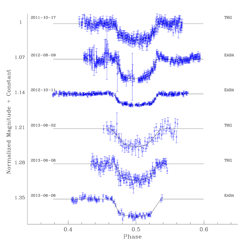
Figure 1: Light-curves presented in this work. The photometric observations and their error-bars are in blue. Black solid lines represent the best-fit to the data. For each transit, the date and the telescope are indicated.

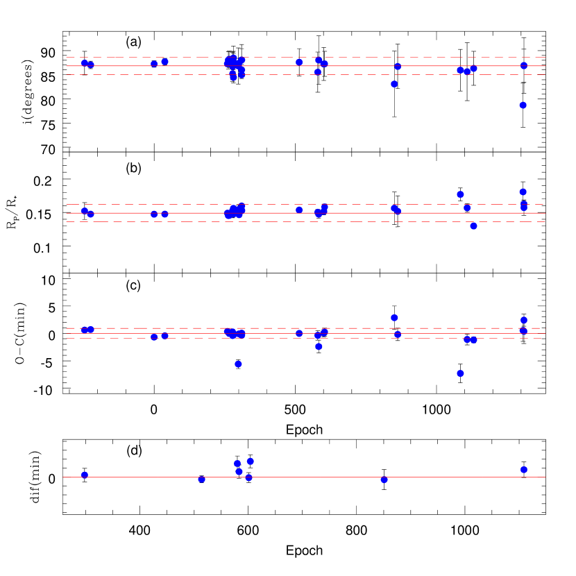
Figure 2: Figures a, b and c: $i$, $R_{P}/R_{\star}$ and $O-C$ as a function of the transit epoch. Blue points are the values obtained for the 34 light curves. The solid and dashed horizontal red lines represent the weighted average and its $\pm 1\sigma$ errors, respectively. Figure d: Differences between the central transit times obtained with the model used in the ETD and the ones obtained in this work.

.

Table 1: Log of our observations

Date	Telescope	Camera	Filter	Bin-size	Exposure-Time (s)	$N_{obs}$	$\sigma$(mag)
Oct 17 2011	THG	U16M	no filter	1x1	25	315	0.0059
Aug 9 2012	EABA	U9	no filter	1x1	40-50	306	0.0069
Oct 11 2012	EABA	U9	R	2x2	25	272	0.0019
Jun 2 2013	THG	U16M	R	2x2	180	68	0.0090
Jun 6 2013	THG	U16M	R	2x2	45	90	0.0063
Jun 6 2013	EABA	U9	R	2x2	90	141	0.0035

Table 2: Physical properties of the star and the exoplanet derived in this work for the 34 light curves

Epoch	Date	$i$($\arcdeg$)	$M_{P}$ ($M_{Jup}$)	$R_{P}$ ($R_{Jup}$)	$g_{P}$ [m/s2]	$T^{\prime}_{eq}$ (K)	$M_{\star}$ ($M_{\odot}$)	$R_{\star}$ ($R_{\odot}$)	$\log g_{\star}$ [cm/s]	Age (Gyr)	a (AU)	Author
-246	2007-09-25	87.42 $\pm$ 2.46	1.22 $\pm$ 0.032	1.349 $\pm$ 0.088	16.6 $\pm$ 2.8	1657 $\pm$ 56.5	0.894 $\pm$ 0.031	0.915 $\pm$ 0.052	4.467 $\pm$ 0.048	5.1 $\pm$ 3	0.02289 $\pm$ 0.00026	1
-225	2007-10-07	87.05 $\pm$ 0.76	1.218 $\pm$ 0.03	1.31 $\pm$ 0.028	17.5 $\pm$ 1.4	1657 $\pm$ 22.5	0.891 $\pm$ 0.029	0.914 $\pm$ 0.015	4.466 $\pm$ 0.012	5.5 $\pm$ 3	0.02287 $\pm$ 0.00025	2
0	2008-08-19	87.23 $\pm$ 0.68	1.215 $\pm$ 0.031	1.323 $\pm$ 0.028	17.2 $\pm$ 1.4	1666 $\pm$ 23.5	0.888 $\pm$ 0.03	0.923 $\pm$ 0.015	4.456 $\pm$ 0.012	6.8 $\pm$ 3	0.02284 $\pm$ 0.00026	3
38	2008-10-09	87.72 $\pm$ 0.72	1.226 $\pm$ 0.034	1.314 $\pm$ 0.025	17.5 $\pm$ 1.3	1654 $\pm$ 22.9	0.9 $\pm$ 0.033	0.914 $\pm$ 0.014	4.471 $\pm$ 0.01	5.1 $\pm$ 3.1	0.02294 $\pm$ 0.00028	3
260	2009-08-02	87.29 $\pm$ 0.59	1.217 $\pm$ 0.028	1.329 $\pm$ 0.023	17 $\pm$ 1.2	1660 $\pm$ 19	0.891 $\pm$ 0.026	0.918 $\pm$ 0.012	4.462 $\pm$ 0.009	5.7 $\pm$ 2.7	0.02286 $\pm$ 0.00022	4
263	2009-08-06	88.03 $\pm$ 1.80	1.218 $\pm$ 0.03	1.291 $\pm$ 0.027	18.1 $\pm$ 1.4	1656 $\pm$ 21.1	0.892 $\pm$ 0.028	0.914 $\pm$ 0.014	4.467 $\pm$ 0.01	5.3 $\pm$ 2.8	0.02287 $\pm$ 0.00024	4
266	2009-08-10	88.21 $\pm$ 1.70	1.217 $\pm$ 0.031	1.291 $\pm$ 0.037	18.1 $\pm$ 1.7	1656 $\pm$ 24.4	0.891 $\pm$ 0.03	0.913 $\pm$ 0.016	4.467 $\pm$ 0.013	5.4 $\pm$ 3	0.02286 $\pm$ 0.00026	4
278	2009-08-26	86.72 $\pm$ 3.07	1.206 $\pm$ 0.035	1.355 $\pm$ 0.111	16.2 $\pm$ 3.3	1680 $\pm$ 52.8	0.877 $\pm$ 0.032	0.934 $\pm$ 0.047	4.44 $\pm$ 0.043	8.8 $\pm$ 2.5	0.02274 $\pm$ 0.00028	5
278	2009-08-26	87.63 $\pm$ 2.23	1.219 $\pm$ 0.031	1.325 $\pm$ 0.083	17.2 $\pm$ 2.8	1664 $\pm$ 43.5	0.893 $\pm$ 0.03	0.922 $\pm$ 0.038	4.46 $\pm$ 0.035	5.9 $\pm$ 2.6	0.02288 $\pm$ 0.00026	5
278	2009-08-26	85.23 $\pm$ 1.60	1.195 $\pm$ 0.035	1.447 $\pm$ 0.087	14.1 $\pm$ 2.3	1717 $\pm$ 51	0.863 $\pm$ 0.033	0.971 $\pm$ 0.045	4.399 $\pm$ 0.039	11.2 $\pm$ 3.3	0.02262 $\pm$ 0.00029	5
278	2009-08-26	86.81 $\pm$ 2.81	1.208 $\pm$ 0.03	1.375 $\pm$ 0.068	15.8 $\pm$ 2.1	1677 $\pm$ 41.8	0.879 $\pm$ 0.028	0.932 $\pm$ 0.037	4.443 $\pm$ 0.033	8.5 $\pm$ 2	0.02276 $\pm$ 0.00024	5
281	2009-08-30	88.49 $\pm$ 2.47	1.231 $\pm$ 0.035	1.307 $\pm$ 0.107	17.8 $\pm$ 3.6	1654 $\pm$ 54.6	0.906 $\pm$ 0.033	0.916 $\pm$ 0.049	4.471 $\pm$ 0.046	4.1 $\pm$ 3	0.02299 $\pm$ 0.00028	5
281	2009-08-30	84.47 $\pm$ 1.15	1.195 $\pm$ 0.038	1.461 $\pm$ 0.069	13.8 $\pm$ 1.9	1711 $\pm$ 48	0.862 $\pm$ 0.037	0.964 $\pm$ 0.04	4.406 $\pm$ 0.035	11.3 $\pm$ 3.7	0.02261 $\pm$ 0.00032	5
281	2009-08-30	87.70 $\pm$ 2.14	1.223 $\pm$ 0.037	1.332 $\pm$ 0.093	17 $\pm$ 3.1	1655 $\pm$ 60.1	0.897 $\pm$ 0.036	0.913 $\pm$ 0.054	4.47 $\pm$ 0.051	4.6 $\pm$ 3.4	0.02291 $\pm$ 0.00031	5
281	2009-08-30	86.89 $\pm$ 2.53	1.217 $\pm$ 0.036	1.367 $\pm$ 0.069	16.1 $\pm$ 2.3	1666 $\pm$ 43.4	0.89 $\pm$ 0.034	0.923 $\pm$ 0.036	4.457 $\pm$ 0.033	6.8 $\pm$ 3.1	0.02285 $\pm$ 0.00029	5
298	2009-09-21	86.83 $\pm$ 3.75	1.206 $\pm$ 0.035	1.402 $\pm$ 0.248	15.1 $\pm$ 6	1687 $\pm$ 136	0.877 $\pm$ 0.032	0.942 $\pm$ 0.14	4.433 $\pm$ 0.13	8.8 $\pm$ 2.6	0.02274 $\pm$ 0.00028	6
301	2009-09-26	87.42 $\pm$ 1.00	1.218 $\pm$ 0.03	1.31 $\pm$ 0.032	17.5 $\pm$ 1.5	1661 $\pm$ 25.9	0.892 $\pm$ 0.029	0.919 $\pm$ 0.019	4.462 $\pm$ 0.016	6.2 $\pm$ 2.6	0.02287 $\pm$ 0.00025	4
310	2009-10-08	88.06 $\pm$ 2.34	1.234 $\pm$ 0.031	1.347 $\pm$ 0.107	16.8 $\pm$ 3.3	1643 $\pm$ 52.8	0.909 $\pm$ 0.029	0.904 $\pm$ 0.048	4.484 $\pm$ 0.046	3.7 $\pm$ 2.4	0.02302 $\pm$ 0.00025	5
310	2009-10-08	84.99 $\pm$ 0.78	1.202 $\pm$ 0.03	1.484 $\pm$ 0.05	13.5 $\pm$ 1.4	1699 $\pm$ 37.8	0.869 $\pm$ 0.029	0.953 $\pm$ 0.032	4.419 $\pm$ 0.028	10.1 $\pm$ 2.6	0.02268 $\pm$ 0.00025	5
310	2009-10-08	86.02 $\pm$ 1.22	1.213 $\pm$ 0.029	1.382 $\pm$ 0.068	15.7 $\pm$ 2.1	1673 $\pm$ 44.5	0.884 $\pm$ 0.027	0.929 $\pm$ 0.04	4.448 $\pm$ 0.037	7.4 $\pm$ 2.3	0.0228 $\pm$ 0.00023	5
310	2009-10-08	88.09 $\pm$ 3.16	1.234 $\pm$ 0.031	1.333 $\pm$ 0.14	17.2 $\pm$ 4.2	1641 $\pm$ 74.2	0.909 $\pm$ 0.029	0.903 $\pm$ 0.072	4.486 $\pm$ 0.069	3.7 $\pm$ 2.3	0.02302 $\pm$ 0.00025	5
514	2010-07-07	87.60 $\pm$ 2.83	1.226 $\pm$ 0.037	1.362 $\pm$ 0.159	16.3 $\pm$ 4.5	1653 $\pm$ 84.3	0.9 $\pm$ 0.036	0.912 $\pm$ 0.081	4.472 $\pm$ 0.077	4.5 $\pm$ 3.5	0.02294 $\pm$ 0.00031	7
580	2010-10-04	85.55 $\pm$ 4.17	1.212 $\pm$ 0.036	1.353 $\pm$ 0.201	16.4 $\pm$ 5.5	1669 $\pm$ 95.8	0.882 $\pm$ 0.031	0.924 $\pm$ 0.095	4.452 $\pm$ 0.089	7.7 $\pm$ 2	0.02279 $\pm$ 0.00027	8
583	2010-10-07	88.05 $\pm$ 5.01	1.232 $\pm$ 0.035	1.293 $\pm$ 0.299	18.2 $\pm$ 9.1	1644 $\pm$ 153.8	0.907 $\pm$ 0.033	0.905 $\pm$ 0.158	4.482 $\pm$ 0.153	4 $\pm$ 2.9	0.023 $\pm$ 0.00028	8
601	2010-11-01	87.24 $\pm$ 3.42	1.231 $\pm$ 0.031	1.336 $\pm$ 0.202	17 $\pm$ 5.8	1651 $\pm$ 143.6	0.905 $\pm$ 0.029	0.912 $\pm$ 0.149	4.475 $\pm$ 0.143	3.6 $\pm$ 2.3	0.02298 $\pm$ 0.00024	9
604	2010-11-05	87.26 $\pm$ 2.60	1.233 $\pm$ 0.03	1.38 $\pm$ 0.155	16 $\pm$ 4.2	1634 $\pm$ 83.6	0.908 $\pm$ 0.028	0.895 $\pm$ 0.082	4.493 $\pm$ 0.08	3.6 $\pm$ 2.3	0.023 $\pm$ 0.00024	8
851	2011-10-01	83.10 $\pm$ 6.80	1.188 $\pm$ 0.06	1.553 $\pm$ 0.796	12.2 $\pm$ 13.2	1779 $\pm$ 265.8	0.85 $\pm$ 0.045	1.037 $\pm$ 0.292	4.336 $\pm$ 0.251	14.6 $\pm$ 1.6	0.02251 $\pm$ 0.0004	6
863	2011-10-17	86.74 $\pm$ 4.62	1.223 $\pm$ 0.029	1.355 $\pm$ 0.235	16.5 $\pm$ 6.3	1672 $\pm$ 171.4	0.895 $\pm$ 0.026	0.932 $\pm$ 0.182	4.451 $\pm$ 0.172	5.2 $\pm$ 1.7	0.0229 $\pm$ 0.00022	10
1085	2012-08-09	85.95 $\pm$ 4.30	1.235 $\pm$ 0.036	1.51 $\pm$ 0.256	13.4 $\pm$ 5.1	1628 $\pm$ 156.1	0.908 $\pm$ 0.031	0.888 $\pm$ 0.16	4.499 $\pm$ 0.158	3.6 $\pm$ 2.2	0.02301 $\pm$ 0.00026	11
1109	2012-09-10	85.64 $\pm$ 6.01	1.202 $\pm$ 0.045	1.457 $\pm$ 0.333	14 $\pm$ 7.1	1698 $\pm$ 213	0.871 $\pm$ 0.039	0.953 $\pm$ 0.225	4.42 $\pm$ 0.209	9.6 $\pm$ 3.1	0.02269 $\pm$ 0.00033	12
1132	2012-10-11	86.34 $\pm$ 3.50	1.204 $\pm$ 0.036	1.202 $\pm$ 0.101	20.6 $\pm$ 4.3	1693 $\pm$ 67.3	0.874 $\pm$ 0.034	0.949 $\pm$ 0.063	4.426 $\pm$ 0.057	9.2 $\pm$ 2.6	0.02272 $\pm$ 0.00029	11
1307	2013-06-02	78.72 $\pm$ 4.56	1.241 $\pm$ 0.111	2.252 $\pm$ 0.477	6 $\pm$ 3.2	1947 $\pm$ 222.6	0.892 $\pm$ 0.108	1.262 $\pm$ 0.238	4.186 $\pm$ 0.163	13 $\pm$ 6.3	0.02287 $\pm$ 0.00092	10
1310	2013-06-06	86.93 $\pm$ 5.76	1.22 $\pm$ 0.035	1.34 $\pm$ 0.359	16.8 $\pm$ 9.7	1661 $\pm$ 155.6	0.894 $\pm$ 0.029	0.92 $\pm$ 0.162	4.462 $\pm$ 0.155	5 $\pm$ 1.8	0.02289 $\pm$ 0.00025	10
1310	2013-06-06	86.89 $\pm$ 3.44	1.196 $\pm$ 0.032	1.53 $\pm$ 0.271	12.6 $\pm$ 5	1712 $\pm$ 126.3	0.867 $\pm$ 0.03	0.966 $\pm$ 0.132	4.406 $\pm$ 0.119	10.8 $\pm$ 2.4	0.02266 $\pm$ 0.00026	11

Note. — (1) Wilson et al. (2008); (2) Gillon et al. (2009); (3) Winn et al. (2009); (4) Sanchis-Ojeda et al. (2011); (5) Nikolov et al. (2012); (6) Tifner (ETD); (7) Sauer (ETD); (8) Curtis (ETD); (9) TgTan (ETD); (10) This work (THG); (11) This work (EABA); (12) Evans (ETD).

Table 3: Final parameters of the WASP-4 system derived in this work

Parameter	Value	Error
Period $P$(days)	1.33823251	0.00000031
Minimum reference Time $T_{0}$($BJD_{TDB}$)	2454697.797973	0.000076
Inclination $i$($\arcdeg$)	86.85	1.76
Stellar Radius $R_{\star}$($R_{\sun}$)	0.92	0.06
Stellar Mass $M_{\star}$($M_{\sun}$)	0.89	0.01
Stellar gravity $\log g_{\star}$($cm/s$)	4.461	0.054
Semimajor axis $a$($UA$)	0.0228	0.00013
Age (Gyr)	7.0	2.9
Stellar effective temperature $T_{eff}$(K)	5436	34
Metallicity $[Fe/H]$(dex)	-0.05	0.04
Planet Radius $R_{P}$($R_{Jup}$)	1.33	0.16
Planet Mass $M_{P}$($M_{Jup}$)	1.216	0.013
Planet surface gravity $g_{P}$($m/s^{2}$)	16.41	2.49
Planet equilibrium temperature $T^{\prime}_{eq}$(K)	1664	54

References

- Beerer et al. (2011) Beerer, I. M., Knutson, H. A., Burrows, A., et al., 2011, ApJ, 727, 23
- Carter & Winn (2010) Carter J. A., & Winn J. N., 2010, ApJ, 716, 850
- Claret (2004) Claret, A., 2004, AA, 428, 1001
- Demarque et al. (2004) Demarque, P., Woo, J. H., Kim, Y. C., Yi, S. K., 2004, ApJS, 155, 667
- Doyle et al. (2013) Doyle, A. P., Smalley, B., Maxted, P. F. L., Anderson, D. R., et al., 2013, MNRAS, 428, 3164
- Eastman et al. (2010) Eastman, J., Siverd, R., Gaudi, B. S., 2010, PASP, 122, 935
- Fortney et al. (2007) Fortney, J. J., Marley, M. S., Barnes, J. W., 2007, ApJ, 668, 1267
- Gillon et al. (2009) Gillon, M., Smalley, B., Hebb, L. et al., 2009, AA, 496, 259
- Girardi et al. (2000) Girardi, L., Bressan, A., Bertelli, G., Chiosi, C., 2000, AAS, 141, 371
- Holman & Murray (2005) Holman, M. J., & Murray, 2005, Science, 307, 1288
- Horne & Baliunas (1986) Horne, J. H., & Baliunas, S. L., 1986, ApJ, 302, 757
- Howell (1989) Howell, S. B., 1989, PASP, 101, 616
- Mandel & Agol (2002) Mandel, K., & Agol, E., 2002, ApJ, 580, 171
- Nascimbeni et al. (2013) Nascimbeni, V., Cunial, A., Murabito, S., et al., 2013, AA, 549, 30
- Nikolov et al. (2012) Nikolov N., Henning T., Koppenhoefer J., et al., 2012, AA, 539, A159
- Pietrinferni et al. (2004) Pietrinferni, A., Cassisi, S., Salaris, M., Castelli, F., 2004, ApJ, 612, 168
- Poddany et al. (2010) Poddany, S., Brat, L., Pejcha, O., 2010, NewAstronomy, 15, 297
- Pont et al. (2006) Pont, F., Zucker S., Queloz, D., 2006, MNRAS, 373, 231
- Press et al. (1992) Press, W. H., Teukolsky, S. A., Vetterling, W. T., Flannery, B. P., 1992. Numerical Recipes in C. The Art of Scientific Computing. University Press, Cambridge.
- Saffe (2011) Saffe, C., 2011, RMxAA, 47, 3
- Sanchis-Ojeda et al. (2011) Sanchis-Ojeda R., Winn J. N., Holman M. J., et al., 2011, ApJ, 733, 127
- Sartoretti & Schneider (1999) Sartoretti P., & Schneider J., 1999, AAS, 134, 553
- Southworth (2009) Southworth, J., 2009, MNRAS, 394, 272
- Southworth (2010) Southworth, J., 2010, MNRAS, 408, 1689
- Southworth et al. (2007) Southworth, J., Wheatley, P. J., & Sams, G., 2007, MNRAS, 379, 11
- Southworth et al. (2009) Southworth, J., Hinse, T. C., Burgdorf, M. J., et al., 2009, MNRAS, 399, 287
- Southworth et al. (2012) Southworth, J., Bruni, I., Mancini, L., Gregorio, J., 2012, MNRAS, 420, 2580
- Southworth et al. (2013) Southworth, J., Mancini, L., Browne, P., et al., 2013, accepted for publication in MNRAS
- Triaud et al. (2010) Triaud, A. H. M. J., et al., 2010, AA, 524, 25
- Van Hamme (1993) Van Hamme, W., 1993, AJ, 106, 2096
- VandenBerg et al. (2006) VandenBerg, D. A., Bergbusch, P. A., Dowler, P. D., 2006, ApJS, 162, 375
- Wilson et al. (2008) Wilson, D. M., Gillon, M., Hellier, C., et al., 2008, ApJ, 675, 113
- Winn et al. (2008) Winn, J. N., Holman, M. J., Torres, G., et al., 2008, ApJ, 683, 1076
- Winn et al. (2009) Winn, J. N., Holman, M. J., Carter, J. A., et al., 2009, AJ, 137, 3826
.