Competition between memory-keeping and memory-erasing decoherence channels

Sommario

We study the competing effects of simultaneous Markovian and non-Markovian decoherence mechanisms acting on a single spin. We show the existence of a threshold in the relative strength of such mechanisms above which the spin dynamics becomes fully Markovian, as revealed by the use of several non-Markovianity measures. We identify a measure-dependent nested structure of such thresholds, hinting at a causality relationship amongst the various non-Markovianity witnesses used in our analysis. Our considerations are then used to argue the unavoidably non-Markovian evolution of a single-electron quantum dot exposed to both intrinsic and Markovian technical noise, the latter of arbitrary strength.

The dynamics of open quantum systems BreuerPbook is of considerable interest both from a fundamental perspective, e.g. for the study of the quantum-to-classical transition Joosetalbook , and for quantum technology. In the latter context, it is important to understand and characterize the effects that an environment has on the quantum features of a given system NielsenCbook . One can distinguish between non-Markovian dynamics, where the coupling with the environment results in the revival of the coherences in the state of the system, and Markovian ones for which no environmental back-action occurs. In many realistic situations, system $\mathcal{S}$ interacts (at different characteristic timescales) with distinct physical environments. This is the case, for instance, for an electron in a quantum dot (QD) that is strongly coupled to the surrounding nuclei and, more weakly, to the phonons of the substrate where it has grown HansonKPTV07 , for a nitrogen-vacancy (NV) center coupled to a bath of spins, embodied by the nitrogen impurities in diamond, where the carbon-13 nuclear spins, on the other hand, couple only weakly to the NV spin Hansonetal08 , and for a single-donor electron spin in silicon Plaeetal12 ; Tyryetal12 , where, thanks to the availability of a isotopically enriched ²⁸Si form without magnetic nuclei, and in presence of a magnetic field gradient, interactions with other donors (with non-zero nuclear magnetic moment) are almost suppressed.

While even the intuitive picture of a non-Markovian process provided above is not universally agreed on and we lack of a general consensus on the very meaning of memory–keeping dynamics in the quantum realm, some theoretical tools have been recently proposed and used to characterize the degree of the non-Markovian nature in the dynamics of open quantum systems. Measures aiming at quantifying any deviation from a Markovian evolution have been put forward BreuerLP09 ; LorenzoPP13 ; RivasHP10 ; LuoFS12 ; bogna and applied to a number of physical situations models , including the first experiments pointing towards the controlled simulation of non-Markovian dynamics experiments .

Notwithstanding a few attempts aimed at finding a unification and an ordering for such a variety of tools BreuerLP09 ; Chruciski1KR11 ; HaikkaCM11 , and apart from the simple case in which only a single decoherence channel is present uncanale , where all of the previous proposals are essentially equivalent, a conclusive picture has yet to be found. In this work we perform some significant steps in this direction by considering the effects of simultaneous environmental mechanisms. Our aim is to investigate open-system dynamics in the presence of competing effects arising because of the simultaneous presence of various channels on a system of interest. We will consider the interaction between the system and an environment ${\mathcal{E}}_{nM}$ that induces strong non-Markovian features, and, at the same time, will assume the system to be also exposed to the influences of a completely forgetful channel ${\mathcal{E}_{M}}$ that, on its own, would be responsible for Markovian evolution. Under these conditions, we determine the amount of a “standard white noise” (enforcing a Markovian behavior) that one needs to add to the given memory–keeping channel in order to let it become fully memoryless.

We show that it is possible to identify precise working conditions under which the system evolution changes from Markovian to non-Makovian and viceversa, thus highlighting the way channels of different nature mutually interfere so as to induce a radical change in the character of a dynamics. This is becoming increasingly important in light of schemes that have been recently proposed for quantum state engineering and quantum control based on non-Markovian evolutions control .

Before entering the core of our analysis, it is beneficial to review shortly the features of the various tools for the analysis of non-Markovianity that have been mentioned above. A common aspect of such quantifiers is that they are expressed in terms of non-Markovianity rates $X_{l}(t)$ (also termed ${\cal N}_{l}$-rates in the following, with label $l$ used to distinguish the various cases that will be addressed below). For Markovian dynamics, these quantities are supposed to stay negative (or constant) in time, while any deviation from negativity signals the non-Markovian nature of an evolution, which is quantified by integrating over the time windows where $X_{l}(t)>0$

$$\mathcal{N}_{l}{=}\int_{X_{l}(t){>}0}X_{l}(t)\leavevmode\nobreak\ {dt}.$$ (1)

A few choices for $X_{l}$ have been made so far BreuerLP09 ; LorenzoPP13 ; RivasHP10 ; LuoFS12 , implying that different evidences of non-Markovianity can be gathered from the very same dynamics: The measure proposed in Ref. BreuerLP09 , denoted here as ${\cal N}_{BLP}$, is based on the observation that a non-Markovian evolution induces a non-increasing behavior of the state distinguishability. In Ref. LorenzoPP13 , some of us proposed to consider $X_{LPP}{=}\partial_{t}{\left|\left|{F}\right|\right|}$, where ${F}$ is the affine transformation of the Bloch vector of the system induced by a dynamical map and $\left|\left|{F}\right|\right|$ is the absolute value of its determinant. The corresponding measure ${\cal N}_{LPP}$ is based on the assumption that a Markovian dynamics induces a monotonic shrinking of the volume of accessible states of $\mathcal{S}$. According to Ref. RivasHP10 , Markovianity is equivalent to the divisibility of the dynamical map $\Phi_{(t,0)}$ (defined so that $\rho^{\cal S}_{t}=\Phi_{(t,0)}\rho^{\cal S}_{0}$, where $\rho^{\cal S}_{t}$ is the state of the system at time $t$).

Writing $\Phi_{(t+\tau,0)}=\Phi_{(t{+}\tau,\tau)}\circ\Phi_{(t,0)}$ with $\circ$ standing for the composition of two maps, Markovianity is mathematically translated into the condition that $\Phi_{(t+\tau,t)}$ should be a completely positive and trace preserving (CPT) map for all $t$ and $\tau$. This implies that one can relate the integrand of ${\cal N}_{RHP}$ in Eq. (1) to the deviation from positivity of the Choi matrix (isomorphic to the map $\Phi_{t{+}\tau,\tau}$). Finally, in Ref. LuoFS12 Markovianity is synonymous of monotonic decrease of the mutual information between the system and an ancilla whose joint initial state is maximally entangled.

Let us now consider a system ${\mathcal{S}}$ interacting with two environments, ${\mathcal{E}_{M}}$ and ${\mathcal{E}}_{nM}$ under the assumption that, if ${\mathcal{S}}$ interacted only with the former (latter), its dynamics would be Markovian (non-Markovian). In order to fix the ideas, we consider both ${\cal S}$ and ${\cal E}_{nM}$ embodied by a spin-${1}/{2}$ particle. The action of the environment ${\cal E}_{M}$ on the state $\rho_{t}$ of the ${\cal S}$-${\cal E}_{nM}$ system is described by the master equation $\dot{\rho}_{t}{=}{-}i[{\hat{\cal{H}}},{\rho_{t}}]+{\mathcal{L}}_{t}\rho_{t}$, where $\hat{\cal H}$ is the Hamiltonian describing the ${\cal S}$-${\cal E}_{nM}$ dynamics and ${\cal L}_{t}$ is the Liouville super-operator

$${\mathcal{L}}_{t}\rho_{t}{=}\sum_{k,j{=}1}^{3}\!\!\frac{\gamma_{kj}}{2}\left([\hat{\sigma}^{\cal S}_{k},\rho_{t}{{\hat{\sigma}}^{{\cal S}\dagger}_{j}}]{+}[{\hat{\sigma}}^{\cal S}_{k}\rho_{t},{{\hat{\sigma}}^{{\cal S}\dagger}_{j}}]\right)$$ (2)

that describes the Markovian dynamics that would be enforced by ${\cal E}_{M}$ only. Here, $\hat{\sigma}^{\cal S}_{j}$ is the $j$-Pauli matrix of $\cal S$ ($j=x,y,z$), and $\gamma_{kj}$ are the entries of the (hermitian) Kossakowski matrix ${\bm{\gamma}}$ GKS ; Daffer . The dynamical map corresponding to the master equation above is completely positive for ${\bm{\gamma}}\geq 0$. In what follows, we will restrict our attention to Kossakowski matrices taking the form ${\bm{\gamma}}{=}{{\left(\begin{matrix}\gamma_{x}&\alpha{+}i\beta&0\\ \alpha{-}i\beta&\gamma_{y}&0\\ 0&0&\gamma_{z}\end{matrix}\right)}}$. Although this choice does not embody the most general case, it encompasses several relevant quantum channels RomeroLF12 . For instance, for $\alpha=\beta=0$ we have a Pauli channel cerf , while an amplitude damping channel is retrieved for $\alpha=\gamma_{z}=0$ with $\beta=2\gamma_{x,y}{=}\gamma$ NielsenCbook .

Finally, we take the $\cal S$-${\cal E}_{nM}$ interaction to be of the Ising-type, $\hat{\cal{H}}{=}({J}/{2})\hat{\sigma}_{A}^{z}\hat{\sigma}_{{\cal E}_{nM}}^{z}$ and, from now on, use the exchange constant $J$ as our frequency unit. This choice allows us to provide an interesting analysis without introducing unnecessary complications inherent in other coupling models, and, in addition, it links to the experimental scenarios we are going to address.

The reduced dynamics of $\cal S$, described by the dynamical map $\rho^{\cal S}_{t}{=}\phi_{t}(\vec{\gamma},\alpha,\beta)\rho^{\cal S}_{0}$ (with $\rho^{\cal S}_{t}{=}{\rm Tr}_{{\cal E}_{nM}}[\rho_{t}]$) is completely characterized by the choice of the entries of ${\bm{\gamma}}$, here identified by the vector $\vec{\gamma}{=}(\gamma_{x},\gamma_{y},\gamma_{z})$ and by the parameters $\alpha$ and $\beta$. As initial conditions, we consider the factorized state $\rho_{0}{=}\rho^{\cal S}_{0}{\otimes}\rho^{{\cal E}_{nM}}_{0}$ with $\rho^{\cal S}_{0}{=}{{\begin{pmatrix}A^{++}_{0}&A^{+-}_{0}\\ A^{-+}_{0}&A^{--}_{0}\end{pmatrix}}}$ and $\rho^{{\cal E}_{nM}}_{0}{=}{{\begin{pmatrix}B^{++}_{0}&B^{+-}_{0}\\ B^{-+}_{0}&B^{--}_{0}\end{pmatrix}}}$, both written in the basis $\{\left|\pm\right\rangle\}$ of eigenstates of $\hat{\sigma}_{z}$. Due to the form of the coupling chosen above, a prominent role will be played by the initial magnetization of ${\cal E}_{nM}$. We therefore introduce the parameter $z{=}2B^{--}_{0}{-}1$. The evolved state of the system has matrix elements

$$A^{++}_{t}=\sum_{p=\pm}A^{pp}_{0}\left(\frac{f_{t}^{p}}{2}-\frac{\beta f_{t}^{-}}{\gamma_{x}{+}\gamma_{y}}\right),$$ (3)

$$A^{+-}_{t}=A^{+-}_{0}[\text{Ch}{+}i\,z\,\text{Sh}]{+}A^{-+}_{0}(\gamma_{x}{-}\gamma_{y}-2i\alpha)\text{Sh}$$

where we have introduced the functions $f_{t}^{\pm}{=}1{\pm}e^{-2(\gamma_{x}{+}\gamma_{y})t}$ that account for the dissipative action of ${\cal E}_{M}$, and the short-cut notation $\{\text{Ch},\text{Sh}\}{=}e^{{-}(\gamma_{x}{+}\gamma_{y}{+}2\gamma_{z})t}\{\cosh\xi t,\frac{\sinh\xi t}{\xi}\}$ with $\xi{=}\sqrt{(\gamma_{x}{-}\gamma_{y})^{2}{+}4\alpha^{2}{-}1}$. These embody both the decoherence induced by ${\cal E}_{M}$ and the (non-Markovian) dynamics due to the coupling with $\mathcal{E}_{nM}$. The populations of $\rho^{\cal S}_{t}$ do not depend on the parameters of $\hat{\mathcal{H}}$ nor on $\rho^{{\cal E}_{nM}}_{0}$ due to the fact that the $\cal S$-${\cal E}_{nM}$ coupling is dissipationless. In addition, the coherences are symmetric under the exchange of $B^{--}_{0}$ with $B^{++}_{0}$ (or $z$ with $-z$) and viceversa.

With the dynamical map $\phi_{t}(\vec{\gamma},\alpha,\beta)$, we can now evaluate some of the measures of non-Markovianity recalled above. Let us start with the isotropic depolarizing channel acting on $\cal S$. This is set by taking $\gamma_{x}{=}\gamma_{y}=\gamma_{z}=\gamma_{0}/4$ and ${\alpha,\beta}=0$. In this case, we can provide compact analytical expressions for the ${\cal N}$-rates $X_{l}$ at the core of Eq. (1) for the four measures discussed above. We find

$$X_{BLP} =\partial_{t}|G_{t}|,\,\,\,\,\,X_{LPP}=\partial_{t}\left[(2f_{t}{-}1)|G_{t}|^{2}\right],$$ (4)

$$X_{RHP} =\lim_{\tau\to 0^{+}}\frac{1}{2\tau}\left(g(t,\tau){-}f_{\tau}{+}\left|g(t,\tau){-}f_{\tau}\right|\right),$$

$$X_{LFS} {=}\partial_{t}[2{+}2h(1{-}f_{t})+\sum_{s{=}\pm}h(f_{t}{+}s|G_{t}|)],$$

where $h(x){=}(x/2)\log_{2}(x/2)$, $G_{t}{=}\sum_{p{=}\pm}e^{-\gamma_{0}t{+}ipt}B^{pp}_{0}$, $f_{t}{=}{(1{+}e^{-\gamma_{0}t})}/{2}$, and $g(t,\tau){=}\left|{G_{t+\tau}}/{G_{t}}\right|$. The dynamics of $\cal S$ is non-Markovian for any pair $(\gamma_{0},z)$ such that the quantities in Eqs. (4) are positive. For the $N_{RHP}$ measure, this condition leads to

$$\mu(z,t,\gamma_{0})\equiv\gamma_{0}{+}\frac{(1-z^{2})\sin(2t)}{1-(1-z^{2})\sin^{2}t}{<}0.$$ (5)

As the function $\mu(z,t,\gamma_{0})$ is even in $z$, we can take $z{\in}\left(0,1\right]$, and obtain $\gamma_{RHP}^{*}{=}(1{-}z^{2})/{z}$ as a threshold for the onset of Markovianity.

This means that $\mathcal{N}_{RHP}{=}0$ and the dynamics is Markovian for all $\gamma_{0}\geq\gamma_{RHP}^{*}$. The case of $z{=}0$, associated with equal diagonal entries in $\rho^{{\cal E}_{nM}}_{0}$, deserves special attention as in this case $\gamma_{RHP}^{*}\to\infty$, implying that the reduced dynamics will always be non-Markovian, regardless of the strength of the coupling between $\cal S$ and ${\cal E}_{M}$. Following a similar procedure we find the thresholds for the BLP and LPP measures as $\gamma_{BLP}^{*}{=}(3/2)\gamma_{LPP}^{*}=(1{-}z^{2})/2z$.

Apart from the thresholds in the depolarizing rates, we can also compare the time windows in which the ${\cal N}$–rates are positive and the non-Markovian nature of the dynamics explicitly appears. These are the time intervals effectively contributing to the integral of Eq. (1). For the first three measures these can be cast into the form $\tan{t}^{+}_{m}\in[y^{-}_{m},y^{+}_{m}]$, where $y^{\pm}_{m}{=}({b_{m}{\pm}\sqrt{b^{2}_{m}{-}4z^{2}}})/{2z^{2}}$, $m$ is a label identifying the various measures, and

$$b_{RHP}=2b_{BLP}{=}3b_{LPP}{=}{2(z^{2}-{}1)}/{\gamma}.$$ (6)

Differently from the other ${\cal N}$–rates, $X_{LFS}$ does not allow for an analytical treatment, and both the threshold for Markovianity onset and the time window have been evaluated numerically, see Fig. (1). It is interesting to notice that for the $N_{LFS}$ measure there is a critical value of the rate $\gamma$ beyond which the evolution of $\cal S$ is Markovian regardless of the value of $z$. This feature is unique of such measure, as the remaining ones allow for values of $(\gamma,z)$ such that the dynamics remains non-Markovian for any $\gamma$.

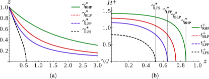
Figura 1: (Color online) (a) Markovianity phase diagram in the $(\gamma,z)$-plane. In the region above (below) each curve, the dynamics of $\mathcal{S}$ is Markovian (non-Markovian) according to the corresponding measure. (b) Hierarchy of the time windows giving contributions to Eq. (1). In the cases corresponding to the three upper curves, the time evolution is periodic, and positivity intervals recur in time. For the LPS measure, due to lack of periodicity, we only report the first positivity interval, noticing that the subsequent intervals all stay below the $t^{+}_{LPP}$ curve.

The results presented so far are fully consistent with what is found by using a time-local master equation for the reduced dynamics of $\mathcal{S}$. By following the approach outlined in Ref. AnderssonCH07 , this reads

$$\dot{\rho}^{\cal S}_{t}{=}{-}i[{\lambda\hat{\sigma}^{\cal S}_{z}},{\rho}^{\cal S}_{t}]{+}\!\!\!\sum_{i{=}\pm,z}\!\!\Gamma_{i}(t)\!\left([\hat{\sigma}^{\cal S}_{i},\rho_{t}{{\hat{\sigma}}^{{\cal S}\dagger}_{i}}]{+}[{\hat{\sigma}}^{\cal S}_{i}\rho_{t},{{\hat{\sigma}}^{{\cal S}\dagger}_{i}}]\right),$$ (7)

where we introduced the ladder operators $\hat{\sigma}^{\cal S}_{\pm}{=}(\hat{\sigma}^{\cal S}_{x}{\pm}i\hat{\sigma}^{\cal S}_{y})/2$, the parameters $\Gamma_{\pm}(t){=}\gamma$ and $\Gamma_{z}(t){=}\frac{1}{2}[\gamma{-}\frac{(z^{2}{+}1)\sin(2t)}{1-(1-z^{2})\sin^{2}t}]$, and the frequency shift $\lambda$ for the system. The map generated by Eq. (7) is non-Markovian when $\Gamma_{z}(t){<}0$, which yields the very same threshold as $\gamma^{*}_{RHP}$.

We have thus found a hierarchy of non-Markovianity in the model under study which orders the four measures that we have addressed using the depolarizing-rate thresholds

$$\gamma_{RHP}^{*}\geq\gamma_{BLP}^{*}\geq\gamma_{LPP}^{*}\geq\gamma_{LFS}^{*}.$$ (8)

The equalities hold only for $z{=}1$ [cf. Fig. 1 (a)]. Moreover, as shown in Fig. 1 (b), we have identified a nested structure of the time windows contributing to the integral measures in Eq. (1), showing that

$$t^{+}_{LFS}{\subset}t^{+}_{LPP}{\subset}t^{+}_{BLP}{\subset}t^{+}_{RHP}.$$ (9)

While highlighting in a clear and original way the inherent differences in the various measures that we have considered, each addressing a different facet of non-Markovianity, this result paves the way to the analysis of other dynamical models, in an attempt to establish a universal, model-independent hierarchy supplenota . Moreover, all of the measures discussed here share the same extremal behavior w.r.t. the initial population of the non-Markovian environment $\mathcal{E}_{nM}$, i.e., at $z{=}1$ all measures give zero, whereas at $z{=}0$ they achieve their maximum values. Remarkably, at this point, the dynamics of $\mathcal{S}$ cannot be made Markovian by adding isotropic depolarizing noise for any value of the decay rate according to three of the measures here employed. On the contrary, the LFS measure gives the threshold $\gamma^{*}\sim 0.6$ for the onset of Markovian dynamics. Finally, a further common feature to all the measures here addressed is that the non-Markovian behavior of the open system is enhanced by increasing the degree of mixedness of $\mathcal{E}_{nM}$.

In order to establish a link between the features discussed here and a situation of experimental relevance, we discuss the case of a single electron quantum dot (QD) HansonKPTV07 ; Urbaszeketal13 , which, inter alia, constitutes one of the most promising platforms for quantum information processing ima ; KloeffelL13 . While the electron constitutes the open system $\mathcal{S}$, the nuclear spins surrounding it might embody an instance of $\mathcal{E}_{nM}$. Moreover, stray phonon excitations due to impurities in the substrate onto which the dot has grown provide an environment that is large enough and sufficiently weakly coupled to $\cal S$ to be responsible for a Markovian channel HansonKPTV07 . In the following, to fix the ideas, we will refer to the case of a semiconductor quantum dot of the II-VI group, such as, e.g., CdTe/ZnTe or Cd/Se QDs Wu10 ; LeGalletal12 ; Guptaetal99 . However, our results are fully general, do not depend on the specific instance of physical system at hand, and can be applied to other similar physical situations which are described by the central-spin model, such as the NV^--center at large magnetic fields (Supplementary Material of Ref. Hansonetal08 ), and a single electron spin phosphorus donors in isotopically enriched ²⁸Si crystal with a reduced abundance of ²⁹Si Tyryetal12 ; WitzelDS06 .

The interaction of the electron spin loaded into the quantum dot with the nuclear ones is described by the Fermi contact hyperfine Hamiltonian $\hat{\cal H}_{\mathcal{S},\mathcal{E}^{nM}}{=}\sum_{n{=}1}^{N}J_{n}\hat{\bm{\sigma}}{\cdot}\hat{\bm{I}}^{n}$, where $I{=}\frac{1}{2}$ for the $N{\simeq}10^{3}$ nuclei in the QD. The coupling strength is proportional to the electronic envelop wavefunction $\left|\psi\left(\bm{r}_{n}\right)\right|^{2}$ at the $n^{\rm th}$ nuclear position. Without loss of generality for our purposes, we use the so-called box model for the electronic wave function $\left|\psi\left(\vec{r}_{n}\right)\right|^{2}{=}{1}/{V}$ (with $V$ the volume occupied by the QD), which implies homogeneous electron-nucleus couplings. We assume that a strong magnetic field is applied to the QD so that we can legitimately retain the sole longitudinal coupling. By introducing the collective operator $\hat{\bm{\mathcal{I}}}{=}\sum_{n{=}1}^{N}\hat{\bm{I}}^{n}$ for the nuclear spins and invoking the rotating-wave approximation, the interaction Hamiltonian takes an Ising-like form $\hat{\cal H}{=}J\hat{\sigma}^{z}\hat{\mathcal{I}^{z}}$ HansonKPTV07 ; Tayloretal07 . In the mean-field approach, the fluctuations of the nuclear magnetic field along the $z$-axis, commonly known as Overhauser field Urbaszeketal13 , are responsible for the dephasing of the electron-spin state KhaetskiiLG02 . The typical timescale for such an effect is $T_{2}\simeq 2.5\unit{ns}$ at zero magnetic field Guptaetal99 as a result of the averaging over many Overhauser field configurations. However, in the presence of strong external magnetic fields and with the application of dynamical-decoupling techniques, coherence times $T_{2}$ up to seconds have have been achieved experimentally Awschalometal13 . In the following, we assume such conditions of negligible nuclear-spin-induced dephasing. As an additional remark, we notice that dissipation induced by the relaxation of nuclear spins due to the dipole-dipole interaction (which is not total angular momentum conserving) occurs at much longer timescales $T_{1}$ MerkulovER02 .

Within these assumptions, the only environmental effects on the electron spin should be ascribed to fluctuating electrical fields caused by or by technical noise (fluctuating gate potentials, spurious background charges or fabrication defects). In the following we show that, even if these noise sources could be modelled by Markovian mechanisms, the dynamics of the electron will never be Markovian.

The dynamics of the open system coupled to $N$ mutually non-interacting spins as described above, under the assumption of a general environmental action characterized by the depolarising parameter $\gamma$, yields the same map $\rho^{\mathcal{S}}_{t}{=}\phi_{t}\rho^{\mathcal{S}}_{0}$ reported above. Here, however, we have $G_{t}{=}e^{-\gamma t}{\rm Tr}[e^{-i\hat{\mathcal{I}}^{z}t}\rho^{{\cal E}_{nM}}]$, where $\hat{\mathcal{I}}^{z}{=}\sum_{n=1}^{N}\hat{I}^{z}_{n}$ is the collective nuclear spin operator along the $z$-axis, $\rho^{{\cal E}_{nM}}$ is the density matrix of the $N$ spins that make up $\mathcal{E}_{nM}$ and we took again $J$ as a frequency unit. Although this expression can be evaluated for any environmental spin state, here we restrict our attention to the experimentally motivated case of $\rho^{{\cal E}_{nM}}{=}\otimes^{N}_{p=1}\rho_{nM}^{p}$. In this case, the single-spin state $\rho_{{nM}}^{p}$ is the same regardless of $p$. These assumptions entail

$${\rm Tr}[e^{-i\hat{\mathcal{I}}^{z}t}\rho^{{\cal E}_{nM}}] {=}\!\sum_{k{=}0}^{N}\!\binom{N}{k}\!\frac{e^{-iI^{z}t\left(2k-N\right)}}{2^{N}}({1\!+\!z})^{k}({1\!-\!z})^{N-k}$$ (10)

$${=}\left[\cos t+iz\sin t\right]^{N},$$

where $k$ is the number of environmental spins in the $\left|0\right\rangle$ state. A straightforward calculation shows that the threshold for the onset of Markovian dynamics increases linearly with $N$ as $\gamma_{{N}_{RHP}}^{*}{=}N\gamma_{RHP}^{*}$, whereas the time intervals at which $\partial_{t}{X}{>}0$ in Eq. (1) shrinks due to $b_{RHP}{=}2N\left(z^{2}{-}1\right)/\gamma$. Considering that, within the range of temperatures typical for quantum dots, $\rho^{{\cal E}_{nM}}{=}2^{-N}{\openone}$, i.e., $z{=}0$, we obtain the remarkable result that the open system dynamics of the dot cannot be made Markovian by adding a Markovian noise of whatever rate. In addition, for $N{\rightarrow}\infty$, we obtain $\mathcal{N}_{RHP}{=}1$, $\mathcal{N}_{BLP}{=}(e^{\pi\gamma}-1)^{-1}$ and $\mathcal{N}_{LPP}=(e^{3\pi\gamma}-1)^{-1}$, meaning that the dynamics of $\cal S$ is non-Markovian for any initial state of $\mathcal{E}_{nM}$ that is not an eigenstate of $\hat{\mathcal{I}}^{z}$. As seen above, for $z{=}1$ the reduced dynamics is Markovian regardless of $\gamma$ and $N$.

We have investigated the behavior of the open-system dynamics of a spin-$\frac{1}{2}$ subject to the competing action of Markovian and non-Markovian environments, identifying the conditions under which the system evolution becomes Markovian. These account in well defined thresholds in the the relative strength of the coupling of the system to the various environments. A nested hierarchical structure then results for the measures of non-Markovianity that we have considered, which suggests a causality relation amongst the different physical phenomena used to characterize non-Markovianity in this context. Our findings might be used to acquire information on the open-system dynamics of a single-electron QD for which, under fairly reasonable assumptions, a Markovian description of the dynamics turns out to be fully inadequate.

Acknowledgments.– TJGA and CDF thank L.  Mazzola and A.  Xuereb for useful discussions. TJGA is supported by the European Commission, the European Social Fund and the Region Calabria through the program POR Calabria FSE 2007-2013-Asse IV Capitale Umano-Obiettivo Operativo M2. MP thanks the UK EPSRC (grant nr. EP/G004579/1), the Alexander von Humboldt Stiftung, and the John Templeton Foundation (grant ID 43467) for financial support.

Appendix: analysis of other decoherence channels

In this Appendix we extend the analysis presented in the main text to the case of a more general decoherence channel given by a combination of an amplitude damping and a depolarizing ones. The resulting channel is characterized by the Kossakowski matrix

$${\bm{\gamma}}{=}\begin{pmatrix}\gamma_{A}&i\gamma_{A}/2&0\\ {-}i\gamma_{A}/2&\gamma_{A}&0\\ 0&0&0\end{pmatrix}+\begin{pmatrix}\gamma_{D}&0&0\\ 0&\gamma_{D}&0\\ 0&0&\gamma_{D}\end{pmatrix}.$$ (11)

The case $\gamma_{A}=0$ has been already analized in the main text. In the presence of the amplitude damping component, the explicit expressions for the ${\cal N}$-rates are analogous to the ones reported in the main text in Eq. (4). By introducing $f_{t}^{\pm}=1\pm e^{-4(\gamma_{A}+\gamma_{D})t}$ we have

$$X_{BLP} =\partial_{t}|G_{t}|,$$ (12)

$$X_{LPP} =\partial_{t}[(f^{+}_{t}{-}1)|G_{t}|^{2}],$$

$$X_{RHP} =\lim_{\tau\to 0^{+}}\frac{1}{2\tau}\left(g(t,\tau){-}\frac{f^{+}_{\tau}}{2}{+}\left|g(t,\tau){-}\frac{f^{+}_{\tau}}{2}\right|\right),$$

$$X_{LFS} {=}\partial_{t}{\cal I}(\sigma),$$

where $\mathcal{I}(\sigma)$ stands for the Quantum mutual information of the matrix

$$\sigma=\frac{1}{4}\begin{pmatrix}f^{+}_{t}{-}\frac{\Upsilon}{2}f^{-}_{t}&0&0&2G^{*}_{t}\\ 0&f^{-}_{t}{-}\frac{\Upsilon}{2}f^{-}_{t}&0&0\\ 0&0&f^{-}_{t}{+}\frac{\Upsilon}{2}f^{-}_{t}&0\\ 2G_{t}&0&0&f^{+}_{t}{+}\frac{\Upsilon}{2}f^{-}_{t}\\ \end{pmatrix},$$ (13)

where we have introduced the parameters

$$\Upsilon=\dfrac{\gamma_{A}}{(\gamma_{A}+\gamma_{D})},\leavevmode\nobreak\ \leavevmode\nobreak\ G_{t}=\sum_{p{=}\pm}e^{-2(\gamma_{A}+2\gamma_{D})t{+}ipt}B^{pp}_{0},$$ (14)

$$g(t,\tau)=\sqrt{\left(\frac{\beta}{4}f^{-}_{\tau}\right)^{2}+\left|\frac{G_{t+\tau}}{G_{t}}\right|^{2}}.$$

The dynamics of $\cal S$ turns out to be non-Markovian for any triplet $\gamma_{A}$, $\gamma_{D}$, $z$ such that the quantities in Eqs. (4) are positive. For the ${\cal N}_{RHP}$ measure, this condition leads to the inequality

$$4\gamma_{D}{-}\frac{(z^{2}-1)\sin(2t)}{\cos^{2}t{+}z^{2}\sin^{2}t}{<}0.$$ (15)

As this function does not depend on $\gamma_{A}$, this implies that a Markovian behavior occurs for decoherence rates satisfying the same threshold valid for the sole depolarizing channel.

For the ${\cal N}_{BLP}$ and the $N_{LPP}$ measures, on the other hand, the positivity condition leads to

$$4(\gamma_{A}+m\gamma_{D})+\frac{(1-z^{2})\sin(2Jt)}{\cos^{2}(Jt)+z^{2}\sin^{2}(Jt)}{<}0,$$ (16)

with $m=2$ ($m=3$) for the BLP (LPP) measure. For the BLP case, the onset of Markovian dynamics is found to occur for $\gamma_{A}+2\gamma_{D}{=}(1{-}z^{2})/{2z}$, while the analogous condition for the LPP measure reads $2\gamma_{A}+3\gamma_{D}{=}(1{-}z^{2})/{3z}$. The form taken by the LFS measure does not allow for an analytic expression. Its behavior is shown in Fig. 2 as a function of $\gamma_{A}$ and $\gamma_{D}$, at a set value of $z$, and is compared to the BLP and LPP measures so as to establish a Markovianity phase-diagram valid for the respective measure.

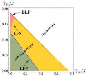
Figura 2: (Color online) Markovianity phase diagram in the $(\gamma_{A},\gamma_{D})$ plane, with $z=0.5$ (other values of the initial magnetization for ${\cal E}_{nM}$ give rise to similar behaviors). The dynamics of the system is Markovian within the colored regions according to the various non-Markovianity measures. The borders of these regions (pointed by the arrows) represent the threshold conditions discussed in the text. The LFS measure has a different behavior for small $\gamma_{A}$, while it tends to coincide with the others quantifiers when the rate of the amplitude damping channel gets larger.

A hierarchical relation among the time windows that contribute to the evaluation of the different indicators can be found here too and leads precisely to the structure given in Eq. (9).