Tuning between singlet, triplet, and mixed pairing states in an extended
Hubbard chain

Abstract

We study spin-half fermions in a one-dimensional extended Hubbard chain at low filling. We identify three triplet and one singlet pairing channels in the system, which are independently tunable as a function of nearest-neighbor charge and spin interactions. In a large-size system with translational invariance, we derive gap equations for the corresponding pairing gaps and obtain a Bogoliubov–de Gennes Hamiltonian with its non-trivial topology determined by the interplay of these gaps. In an open-end system with a fixed number of particles, we compute the exact many-body ground state and identify the dominant pairing revealed by the pair density matrix. Both cases show competition between the four pairing states, resulting in broad regions for each of them and relatively narrow regions for mixed-pairing states in the parameter space. Our results enable the possibility of tuning a nanowire between singlet and triplet pairing states without breaking time-reversal or $SU(2)$ symmetry, accompanied by a change in the system’s topology.

I Introduction

Cooper pairingCooper56 is a key ingredient for exploring condensation, superconductivity and superfluidity in interacting many-fermion systemsLeggett06 . In an electronic system, phonon-mediated pairing between two electrons through a singlet channel accounts for the onset of conventional superconductivity, which is well described by the Bardeen-Cooper-Schrieffer (BCS) theory invented over a half century agoBardeen57 . Since then, pairing mechanisms via different spin and orbital channels have been extensively investigated, resulting early in successful understanding of triplet pair superfluid phases in liquid ³HeAnderson61 ; Balian63 ; Anderson73 ; Leggett75 ; Wheatley75 ; Lee97 ; Leggett06 or later in active studies on a variety of unconventional superconductors such as cupratesSigrist91 ; Dagotto94 ; Tsuei00 ; Demler04 ; Lee06 and iron pnictidesStewart11 ; Chubukov12 ; Seo08 ; Mereo09 ; Wang09 ; Wu ; Hung12 with singlet pairing order parameters as well as several heavy-fermion compoundsJoynt02 ; Pfleiderer09 and strontium ruthenate Sr₂RuO₄Mackenzie03 ; Maeno12 with triplet ones.

Multiple pairing effects enable the possibility of a transition (or crossover) from one energetically favorable pairing state to another as the system parameters change. In a triplet pairing case, superfluid ³He can undergo a first-order phase transition between an equal-spin-pairing state and a specific ${}^{3}P_{0}$ spin-orbit pairing state (³He-$A$ and $B$ phases, respectively)Leggett75 ; Leggett06 , as a function of temperature and pressure. In a singlet pairing case, the BCS-type superconductor or superfluid with a uniform pairing order parameter can undergo a transition to a state with spatially oscillatory ones in the presence of spin imbalance or magnetic field, such as the Fulde-Ferrell-Larkin-Ovchinnikov stateFF ; LO with its experimental evidence in CeCoIn₅ Matsuda07 ; Pfleiderer09 and cold ⁶Li gasesLiao10 , or the theoretically proposed $p$-orbital pair condensateZhang10 . In addition, several exotic transitions between $d$-$(d+is)$-$s$Musaelian96 ; Khodas12 , $(p+ip)$-$p$Gurarie05 and $(p+ip)$-$f$Cheng10 orbital pairing orders have also been theoretically discussed. However, all these cases show the changes of the order parameters only in the orbital or $z$-component spin space, while the total spin of the pairing order remains the same (singlet or triplet) upon the transitions. A transition or crossover between singlet and triplet pairing states was less studied.

Moreover, in three dimensions there is an interesting state showing the coexistence of $s$- and $p$-wave pairing orders (reminiscent of a fragmented condensate), provided the interparticle potentials in triplet and singlet channels are both energetically favorableBalian63 . Such a mixed state survives merely in a restrictive parameter regime and has not been much focusedLeggett75 . In two dimensions, the mixed state has been proposed with the assistance of spin-orbit couplingsGorkov01 , interfacial barriers,Romano13 or deformation in the Fermi surface.Kuboki01 Recent findings have suggested a feasible proposal for this mixture, which is proximity-induced $p$-wave superconductivity in a ferromagnets/$s$-wave superconductor heterostructure Volkov03 ; Bergeret05 ; Keizer06 ; Eschrig08 ; Linder10 ; Almog11 ; Klose12 ; Quarterman12; Leksin12 ; Bergeret13 ; Hikino13 . In these devices, even if the competition between singlet and triplet pairing orders always exists since the attractive interaction between opposite spins accompanies with the desired attractive interaction between same spins, they can coexist within a range across the interface, with thickness comparable to the superconducting coherence length. Nevertheless, the ferromagnet/superconductor interface is strongly inhomogeneous such that the mixed region can hardly be described as a uniform phase. For effectively characterizing the quantum phases with singlet, triplet, and mixed pairing order parameters, a well-defined uniform system and its modeling ought to be further investigated.

Recently, a lot of interest has been stimulated in one-dimensional (1D) superconductors for their topological nontrivial properties and potential application on quantum information processingKitaev01 ; Wilczek09 ; Franz10 ; Alicea12 ; Beenakker13 . In a system of spinless fermions on an open chain, the superconducting state, which has a $p$-wave (triplet) pairing order parameter, has been shown in a given parameter range as a topological state that carries one Majorana fermion on each end of the chainKitaev01 . In a case of spin-half fermions, the Majorana fermion states can emerge within a heterostructure in the presence of $s$-wave (singlet) pairing order, spin-orbit coupling and magnetic Zeeman fieldLutchyn10 ; Oreg10 ; Stoudenmire11 , which has been experimentally realized in semiconductor nanowires having a proximity-induced superconducting gapMourik12 ; Deng12 ; Rokhinson12 ; Das12 ; Finck13 ; Churchill13 . On the other hand, a singlet superconductor without spin-orbit and magnetic couplings is always topologically trivial. Therefore, regarding the equivalence between a spin-half system and two copies of spinless ones in the limit of spin decoupling, one could expect that the tuning between one-dimensional singlet and triplet pairing states may induce a change in the system’s topology and hence provide a new route for topological manipulation. In addition, the topological property of a mixed pairing state would also be an interesting subject. From this point of view, systems with inside tunable pairing channels would be more appropriate for investigation.

In this paper, we study an extended one-dimensional Hubbard model with nearest-neighbor charge and spin interactions, particularly focusing on the pairing phenomena in uniform and low-filling regimes. We show that the system contains all four possible pairing channels in the pair spin space, with coupling strengths that can be independently varied by the tuning of charge and spin interactions. We apply a mean-field treatment on a large-size case with translational invariance and will derive gap equations characterizing two intraspin triplet, one interspin triplet as well as one singlet pairing orders, and mixed regions of them. We shall obtain the effective Bogoliubov–de Gennes (BdG) Hamiltonian of the model and discuss its topological properties. Beyond the mean-field treatment, we perform exact diagonalization on an open-end chain with a fixed number of particles, with modifications to reduce finite-size effects (see detailed discussions in Sec. IV.1). We compute pair fractions of the exact many-body ground state that indicates dominant and stable pair species toward large-size and low-filling regimes (reminiscent of a pair condensate). The results will show a change of dominant pair species from one to another as the corresponding couplings vary, accompanied with a characteristic behavior of pair susceptibility or entanglement entropy. The mixed pairing state will also be identified in regions where more than one pair species dominate. Finally we compare the mean-field and exact-diagonalization results.

The paper is organized as follows. In Sec. II we introduce the model Hamiltonian and phenomenologically discuss the pairing physics in the system. In Sec. III we perform the mean-field treatment on a translation-invariant system to derive the gap equations, followed by discussions of the pairing behavior as well as the topological properties of the system. In Sec. IV we compute the exact ground state of a fixed-number open-end chain. We present data that show evolution of dominant pair species as the function of couplings and plot state diagrams that characterize various stable pairing states including mixed ones. Finally we summarize this study in Sec. V.

II Model

In this section we introduce the model Hamiltonian and phenomenologically discuss the pairing tendency in the system. We begin with an extended 1D Hubbard Hamiltonian with charge as well as spin interactions and represent it in a suggestive form that directly pinpoints four independently tunable pairing channels. We then write down a fixed-number BCS-type ansatz to explain how various pair species energetically compete with each other. Finally we discuss how the system’s symmetry enables a mixed pairing state.

The extended Hubbard model has a general form of

$$\tilde{H}=\sum\limits_{i}\Big{[}{\sum\limits_{\sigma=\uparrow,\downarrow}{-{{t}_{\sigma}}\left({\hat{c}_{\sigma i}^{\dagger}{{\hat{c}}_{\sigma i+1}}+{\rm{H}}{\rm{.c}}{\rm{.}}}\right)-{{\mu}_{\sigma}}{{\hat{n}}_{\sigma i}}}}$$

$$+U{{\hat{n}}_{\uparrow i}}{{\hat{n}}_{\downarrow i}}+\sum\limits_{\sigma,\sigma^{\prime}=\uparrow,\downarrow}{{{V}_{\sigma\sigma^{\prime}}}{{\hat{n}}_{\sigma i}}{{\hat{n}}_{\sigma^{\prime}i+1}}}+4J{{{\bf{\hat{S}}}}_{i}}\cdot{{{\bf{\hat{S}}}}_{i+1}}\Big{]},$$ (1)

where $\hat{c}_{\sigma i}^{\dagger}$ creates a fermion of spin $\sigma$ on site $i$, $\hat{n}_{\sigma i}=\hat{c}_{\sigma i}^{\dagger}\hat{c}_{\sigma i}$ is the number operator, ${\bf{\hat{S}}}_{i}=\hat{c}_{\alpha i}^{\dagger}{\vec{\sigma}}_{\alpha\beta}\hat{c}_{\beta i}/2$ is the spin operator with ${\vec{\sigma}}=\{\sigma^{x},\sigma^{y},\sigma^{z}\}$ being Pauli matrices, $t$ is the nearest-neighbor tunneling strength, and $\mu$ is the chemical potential. The couplings $U$, $V$ and $J$ represent the on-site charge, nearest-neighbor charge, and spin interactions, respectively. The parameters $t$, $\mu$, and $V$tuningV are taken as spin-dependent for the most general case (notice that ${V_{\uparrow\downarrow}}={V_{\downarrow\uparrow}}$ is required for most physical interactions).

In the following, we consider a case in which two spin species are balanced and have the same single-particle spectrum, or $t_{\sigma}\to t$ and $\mu_{\sigma}\to\mu$. We also focus on low-filling regimes in which the double occupancies are dilute such that the onsite repulsion can be treated as effective contributions to the chemical potential in a Hartree approximation, ${{\hat{n}}_{\uparrow i}}{{\hat{n}}_{\downarrow i}}\to\left\langle{{{\hat{n}}_{\downarrow i}}}\right\rangle{{\hat{n}}_{\uparrow i}}+\left\langle{{{\hat{n}}_{\uparrow i}}}\right\rangle{{\hat{n}}_{\downarrow i}}$. However, the nearest-neighbor charge and spin interactions account for intersite correlations that are essential for the pairing behavior (as we will discuss later) and hence can not be decoupled as single-site quantities. (We will show later in this section that the physics of interest does not qualitatively alter even incorporating the onsite interaction as its original form in Eq. (1), no matter whether it is repulsive or attractive.) Therefore, with the approximation for the onsite repulsion, one can pinpoint the pairing channels by rewriting the Hamiltonian of Eq. (1) in a suggestive form using two intrapin triplet pair operators ${\hat{b}_{\sigma,i}^{\dagger}=\hat{c}_{\sigma,i+1}^{\dagger}\hat{c}_{\sigma,i}^{\dagger}}$ for $\sigma=\uparrow,\downarrow$ as well as two interspin triplet and singlet pair operators ${\hat{b}_{\pm,i}^{\dagger}=(\hat{c}_{\downarrow,i+1}^{\dagger}\hat{c}_{\uparrow,i}^{\dagger}\pm\hat{c}_{\uparrow,i+1}^{\dagger}\hat{c}_{\downarrow,i}^{\dagger}})/\sqrt{2}$, respectively, as

$$\hat{H}=\sum\limits_{i}\big{(}\hat{H}^{0}_{i}+\hat{H}^{\rm{I}}_{i}\big{)},$$ (2)

with the non-interacting part,

$$\hat{H}^{0}_{i} ={\sum\limits_{\sigma=\uparrow,\downarrow}{-t\left({\hat{c}_{\sigma i}^{\dagger}{{\hat{c}}_{\sigma i+1}}+{\rm{H}}{\rm{.c}}{\rm{.}}}\right)-\mu{{\hat{n}}_{\sigma i}}}},$$ (3)

and the interacting part,

$$\hat{H}^{\rm{I}}_{i} =\sum\limits_{\alpha=\uparrow,\downarrow,\pm}{{g_{\alpha}}\hat{b}^{\dagger}_{\alpha,i}\hat{b}_{\alpha,i}}.$$ (4)

Here the four pair couplings $g_{\uparrow,\downarrow,\pm}$ are independently tunable via the tuning of the charge and spin interactions ${V_{\uparrow\uparrow}}$, ${V_{\downarrow\downarrow}}$, ${V_{\uparrow\downarrow}}$ and $J$ in Eq. (1) as

$${g_{\uparrow(\downarrow)}} = {V_{\uparrow\uparrow(\downarrow\downarrow)}}+J,$$ (5)

$${g_{+}} = {V_{\uparrow\downarrow}}+J,$$ (6)

$${g_{-}} = {V_{\uparrow\downarrow}}-3J.$$ (7)

The Hamiltonian of Eq. (2) conserves the total number of each spin species $N_{\uparrow(\downarrow)}$. We phenomenologically discuss the pairing tendency by applying a generalized number-conserving BCS ansatznumberconserving on the many-body ground state in the momentum space $k$,

$${{\psi_{{\rm{BCS}}}}=\mathcal{A}{{\prod\limits_{\alpha=\uparrow,\downarrow,\pm}{\left({\sum\limits_{k}{{f_{\alpha,k}}\hat{b}_{\alpha,k}^{\dagger}}}\right)}}^{M_{\alpha}}}}{\left|{{\rm{vac}}}\right\rangle}.$$ (8)

Here the pair operators are defined in terms of Fourier-transformed single-particle operators $\{\hat{c}^{\dagger}_{\alpha,k}\}$, as ${\hat{b}_{\uparrow(\downarrow),k}^{\dagger}=\hat{c}_{\uparrow(\downarrow),k}^{\dagger}\hat{c}_{\uparrow(\downarrow),-k}^{\dagger}}$ and ${\hat{b}_{\pm,k}^{\dagger}=\hat{c}_{\downarrow,k}^{\dagger}\hat{c}_{\uparrow,-k}^{\dagger}\pm\hat{c}_{\uparrow,k}^{\dagger}\hat{c}_{\downarrow,-k}^{\dagger}}$, $f_{\alpha,k}$ is the amplitude for $b_{\alpha,k}^{\dagger}$, ${\left|{{\rm{vac}}}\right\rangle}$ is the vacuum state, and $\mathcal{A}$ is the normalization constant. The total numbers of each pair species $M_{\alpha}$ are subject to number conservation relations $2M_{\uparrow(\downarrow)}+M_{+}+M_{-}={N_{\uparrow(\downarrow)}}$. Such constraints enable an energetic competition between each pair species. From this point of view, we expect the ground state with the favor (disfavor) of intraspin triplet, interspin triplet or singlet pairing [or $M_{\alpha}$ dominates (diminishes)] if the corresponding coupling $g_{\alpha}$ is negative (positive) or attractive (repulsive). From Eqs. (5)–(7) we note that the attractive charge interaction (negative $V$) always benefits pairing. The antiferromagnetic spin coupling (positive $J$) leads to the favor of singlet pairing, as reminiscent of the singlet ($d$-wave) superconducting order in the two-dimensional $t$-$J$ modelLee06 , while the ferromagnetic coupling (negative $J$) favors the triplet pairing, as reminiscent of the proximity-induced $p$-wave superconducting order in ferromagnet-superconductor junctionsVolkov03 ; Bergeret05 ; Keizer06 ; Eschrig08 ; Linder10 ; Almog11 ; Klose12 ; Gingrich12 ; Leksin12 ; Bergeret13 ; Hikino13 . If one considers the onsite interaction $U$ as its original form in Eq. (1), it will energetically contribute only to the singlet pair species. In this case, one could follow the same discussion above for the energetic competition between different pair species, except now the effect considered from the nearest-neighbor singlet coupling $g_{-}$ should be replaced by a combined effect of $g_{-}$ itself and $U$. Therefore, we do not expect a qualitative change in the trend of pairing tendency by incorporating the $U$ term, no matter whether it is attractive or repulsive, and can thus stay with Eq. (2) both for simplicity and without the loss of generality. The ansatz of Eq. (8) also tells that once a pair species is more energetically favorable than the others, its total number tends to maximize. Therefore, only one dominant pairing order is usually expected in a number-conserving system, unless such trend is protected by symmetries as discussed below.

The system possesses time-reversal symmetry if $g_{\uparrow}=g_{\downarrow}$ and $SU(2)$ symmetry if $g_{\uparrow}=g_{\downarrow}=g_{+}$. These symmetries insert a sufficient condition of the coexistence of multiple triplet pairing orders. For example, both intraspin pairing orders should simultaneously emerge in the presence of time-reversal symmetry, and together accompany the interspin triplet one in the presence of $SU(2)$ symmetry. We note that the mixture of the two intraspin pairing orders [e.g., $M_{\uparrow}=M_{\downarrow}\neq 0$ and $M_{\pm}=0$ in Eq. (8)] is different from the interspin triplet pairing state (e.g., $M_{+}\neq 0$ and $M_{\uparrow,\downarrow,-}=0$). The former is a fragmented state (which has more than one dominant pair species), while the latter is spin coherent and known as an equal spin pairing state [${\hat{b}_{+,k}^{\dagger}\to\hat{c}_{\uparrow,k}^{\dagger}\hat{c}_{\uparrow,-k}^{\dagger}+\hat{c}_{\downarrow,k}^{\dagger}\hat{c}_{\downarrow,-k}^{\dagger}}$ after an $SU(2)$ roration], analogous to the liquid ³He-A phase Leggett06 . In the limit of $g_{\pm}\to 0$, the Hamiltonian of Eq. (2) decouples to two independent chains, each of which is described by Kitaev’s spinless fermionic modelKitaev01 in the presence of $U(1)$ symmetry breaking, capable of carrying Majorana fermions in a topologically nontrivial state. Starting from this limit, our model provides a route studying various couplings between such two chains and their evolution toward the singlet pairing (topological trivial) regime, hinting of a topological phase transition. Finally, we remark that triplet and singlet orders can coexist without breaking any of the symmetries discussed above. However, even if they coexist, we expect the mixture in a relatively narrow parameter range where the two pair species are energetically compatible, outside which one order can always overcome the other and become dominant. In Secs. III and IV we use two different methods investigating the competition between the four pairing orders as a function of the four couplings and identifying the dominant regions for each pair species or their mixture.

III Mean-field treatment on a large-size system

In this section, we establish a mean-field treatment for the extended Hubbard Hamiltonian $\hat{H}$ in Eq. (2) with translational invariance (large-size limit) at zero temperature to understand the possibility of triplet and singlet pairings. First, we start from the exact quantum partition function and perform a Hubbard-Stratonovich transformation with one singlet and three triplet auxiliary bosonic fields. After the transformation, we obtain an effective BdG Hamiltonian and turn to discuss its topology with the four pairings. Back to the main track, we derive the gap equations of pairings and then find the parameter range corresponding to the presence of pairing.

Before proceed, we comment that although the mean-field treatment does not incorporate quantum fluctuations, which could be essential for studying the 1D physics, it has been widely applied to describe various 1D superconducting states both qualitatively and quantitatively. For example, the mean-field solutionsMizushima05 ; *Parish07; *Liu07; *Sun11; *Baksmaty11; *Sun12 for 1D spin-imbalanced superconductors well match those obtained from unbiased methodsOrso07 ; *Feiguin07; *Bolech09 and agree with experimental findingsLiao10 . In Appendix A, we consider another supportive example of 1D superconducting systems, the Richardson modelRoman02 ; Dukelsky04 , and show the mean-field solution consistent with the exact one for characterizing the superconducting phase. Moreover, our BdG Hamiltonian, which exhibits interesting topological properties as discussed below, can be effectively applied on nano-wires with proximity-induced superconducting gapsMourik12 ; Deng12 ; Rokhinson12 ; Das12 ; Finck13 ; Churchill13 , producing potential realization of tunable 1D topological superconductors. Therefore, our mean-field study in this section is not only valid to a certain extent but is also useful from both theoretical and practical standpoints.

The quantum partition function of the system can be written as

$$Z=\int\prod_{i}\mathfrak{D}{\bf c}_{i}\mathfrak{D}{\bf c}_{i}^{\dagger}e^{-\int_{0}^{\beta}d\tau[{\bf c}^{\dagger}_{i}\partial_{\tau}{\bf c}_{i}+\hat{H}_{i}^{0}+\hat{H}_{i}^{\rm{I}}({\bf c}_{i},{\bf c}_{i}^{\dagger})]},$$ (9)

where ${\bf c}_{i}=(c_{\uparrow i},c_{\downarrow i})^{T}$. We introduce four bosonic (scalar) auxiliary fields $\rho_{i}=(\Delta_{\uparrow i},\Delta_{\downarrow i},\Delta_{+i},\Delta_{-i})$ corresponding to pairing $b_{\uparrow i},\ b_{\downarrow i},\ b_{+i}$ and $b_{-i}$ respectively to perform a Hubbard-Stratonovich transformation for the partition function

$$Z=\int\big{(}\prod_{p}\mathfrak{D}{\bf c}_{p}\mathfrak{D}{\bf c}_{p}^{\dagger}\big{)}\prod_{i}d\rho_{i}d\rho_{i}^{*}e^{-\int_{0}^{\beta}d\tau({\bf c}^{\dagger}_{i}\partial_{\tau}{\bf c}_{i}+S_{i})},$$

where ${\bf c}_{p}=(c_{\uparrow p},c_{\downarrow p})^{T}$ and

$$S_{i}=\sum_{\alpha=\uparrow,\downarrow,\pm}\left[-\frac{\Delta_{\alpha i}^{*}\Delta_{\alpha i}}{g_{\alpha}}+\Delta_{\alpha i}b^{\dagger}_{\alpha i}+{\rm{H.c.}}\right]+\hat{H}^{0}_{i}.$$ (11)

Although the action gains extra degrees of freedom from the auxiliary fields ($b_{\alpha i}$), the effective Hamiltonian with $b_{\alpha i}$ becomes integrable for ${\bf c}^{\dagger}_{\alpha i}$ and ${\bf c}_{\alpha i}$. Later, ${\bf c}^{\dagger}_{\alpha i}$ and ${\bf c}_{\alpha i}$ will be integrated out, and the pairing gaps $\Delta_{\alpha}$ will be determined by finding the local extremum of the action. Furthermore, understanding the expression of the action in momentum space is necessary to compute the gap equation in the following steps. Before performing Fourier transformation, we assume the auxiliary fields to be translation invariant so the site index $i$ can be neglected. In the momentum space, the partition function with the translation-invariant auxiliary fields is rewritten as

$$\mathbf{Z}=\int\big{(}\prod_{p}\mathfrak{D}{\bf c}_{p}\mathfrak{D}{\bf c}_{p}^{\dagger}\big{)}d\rho d\rho^{*}e^{-\int_{0}^{\beta}d\tau\Big{[}L\sum_{\alpha=\uparrow,\downarrow,\pm}\frac{\Delta_{\alpha}^{*}\Delta_{\alpha}}{g_{\alpha}}+\sum_{p}({\bf c}^{\dagger}_{p}\partial_{\tau}{\bf c}_{p}+\bf C_{p}^{\dagger}H_{p}^{\rm{BdG}}\bf C_{p})\Big{]}},$$ (12)

up to a constant multiplier. Here $L$ is the total number of the system sites,

$$H^{\rm{BdG}}_{p}=\begin{pmatrix}\frac{-2t\cos p-\mu}{2}&0&i\sin p\Delta_{\uparrow}&\frac{-i\sin p\Delta_{+}-\cos p\Delta_{-}}{\sqrt{2}}\\ 0&\frac{-2t\cos p-\mu}{2}&\frac{-i\sin p\Delta_{+}+\cos p\Delta_{-}}{\sqrt{2}}&i\sin p\Delta_{\downarrow}\\ -i\sin p\Delta_{\uparrow}^{*}&\frac{i\sin p\Delta_{+}^{*}+\cos p\Delta_{-}^{*}}{\sqrt{2}}&\frac{2t\cos p+\mu}{2}&0\\ \frac{i\sin p\Delta_{+}^{*}-\cos p\Delta_{-}^{*}}{\sqrt{2}}&-i\sin p\Delta_{\downarrow}^{*}&0&\frac{2t\cos p+\mu}{2}\end{pmatrix},$$ (13)

and $\bf C_{p}=\begin{pmatrix}c_{\uparrow p}&c_{\downarrow p}&c^{\dagger}_{\uparrow-p}&c^{\dagger}_{\downarrow-p}\end{pmatrix}^{T}$ is a vector describing particle and hole variables. The effective Hamiltonian $H^{\rm{BdG}}_{p}$ is identified as the well-known BdG HamiltonianDeGennes66 describing superconducting systems in the momentum space. If all the triplet gaps vanish $\Delta_{\uparrow}=\Delta_{\downarrow}=\Delta_{+}=0$, $H^{\rm{BdG}}_{p}$ return to the BCS pairing case. If $\Delta_{+}$ and $\Delta_{-}$ vanish, the system of $H^{\rm{BdG}}_{p}$ can be treated as two decoupled Kitaev’s 1D chainsKitaev01 , which are time-reversal partners.

Let us return to the parent Hamiltonian in Eq. (2). Before the Hubbard-Stratonovich transformation, the parent Hamiltonian shows that the system preserves time-reversal symmetry given $g_{\uparrow}=g_{\downarrow}$. Although $U(1)$ symmetry is broken after the transformation, the time-reversal symmetry should be preserved in $H^{\rm{BdG}}_{p}$. For spin-half particles, the time-reversal symmetry is defined as $\Theta=is_{y}K$ in the spin space, where $K$ is the complex conjugation operator, such that $c^{\dagger}_{\uparrow}\rightarrow-c^{\dagger}_{\downarrow}$ and $c^{\dagger}_{\downarrow}\rightarrow c^{\dagger}_{\uparrow}$. Therefore, in the hole basis, the time-reversal symmetry is still of the same form. To preserve time-reversal symmetry in $H^{\rm{BdG}}_{p}$, the constraints of the pairing gaps must be imposed:

$$\Delta_{\uparrow}=\Delta_{\downarrow}^{*},\ \Delta_{+}=-\Delta^{*}_{+},\ \Delta_{-}=\Delta^{*}_{-}.$$ (14)

In general, because of the $U(1)$ symmetry breaking, the phase of each pairing gap can be arbitrarily chosen by a $U(1)$ gauge transformation. However, under arbitrary $U(1)$ transformation, the constraints above no longer hold, and the definition of the time-reversal operator $\Theta$ also changes. Hence, to avoid the ambiguities of the unfixed pairings and the expression of $\Theta$, we require the $U(1)$ gauge fixed once the time-reversal-invariant constraints are imposed.

In the following, we turn to investigate the topological phases of the $H_{p}^{\rm{BdG}}$. The BdG Hamiltonian, which possesses particle and hole bases, automatically preserves particle-hole symmetry with the corresponding symmetry operator $\Xi=\sigma_{x}K$, which exchanges particle and hole. On the other hand, for a spin-$1/2$ system, the time-reversal operators obeys $\Theta^{2}=-1$ so this system belongs to the class DIII, which exhibits $\mathbb{Z}_{2}$ topological property in one dimension. To determine the topology of the 1D chain, we first consider a simple case where $\Delta_{+}=\Delta_{-}=0$. The BdG Hamiltonian becomes block diagonalized and each block can be treated as a Kitaev 1D chain. Hence, the system corresponds to two decoupled Kitaev 1D chains. We expect that two Majorana modes arise at each end of the entire 1D non-trivial system. KitaevKitaev01 shows that the nontrivial region is given by $|\mu|<2t$. Now we recover nonzero $\Delta_{+}$ and $\Delta_{-}$ to discuss the topology. In the absence of all triplet pairings, the topological phase of the singlet pairing superconductor is expected to be trivial. This 1D chain is either nontrivial or trivial so the boundary between the two phases is to be determined. The boundary is topological phase transition points where the energy gap is closed. To find the transition points, we write down the energy spectrum of $H^{\rm{BdG}}_{p}$,

$$4E_{\pm}^{2}=\left(2t\cos p+\mu\right)^{2}+\left(\sin p|\Delta_{t}|\pm\cos p|\Delta_{-}|\right)^{2},$$ (15)

where

$$|\Delta_{t}|^{2}= |\Delta_{\uparrow}|^{2}+|\Delta_{\downarrow}|^{2}+|\Delta_{+}|^{2}.$$ (16)

When $E_{\pm}=0$, the transition occurs. That is, ${2t|\Delta_{t}|}/{\sqrt{|\Delta_{-}|^{2}+|\Delta_{t}|^{2}}}=|\mu|$ is the boundary of the non-trivial region. Because $t>|\mu|$ is the nontrivial region in the Kitaev model, the region can be extended to

$$\frac{2t|\Delta_{t}|}{\sqrt{|\Delta_{-}|^{2}+|\Delta_{t}|^{2}}}>|\mu|,$$ (17)

for our model. Here we see that the system is always topologically trivial in a purely singlet pairing state ($\Delta_{-}\neq 0,\Delta_{t}=0$) and has the maximum topologically nontrivial region (the same region as in Kitaev’s model) in a purely triplet pairing state ($\Delta_{-}=0,\Delta_{t}\neq 0$). In a mixed pairing state ($\Delta_{-}\neq 0,\Delta_{t}\neq 0$), the enhancement of the singlet pairing strength shrinks the topologically nontrivial region, which indicates a topological order as a result from the competition between singlet and triplet pairings. Our finding also enables a different route for realizing a topological transition via the tuning of the singlet pairing $|\Delta_{-}|$, given $t$, $\mu$ and the triplet pairing $|\Delta_{t}|$ (the three components in Kitaev’s model) all fixed. The rigorous derivation of the topologically nontrivial region by computing $\mathbb{Z}_{2}$ invariant is provided in Appendix B for interested readers.

Now our focus is back on the partition function $\mathbf{Z}$ to determine the values of the pairings. We integrate out all of the fermion operators $c^{\dagger}_{\beta p}$ and $c_{\beta p}$ in the partition function

$$\mathbf{Z}=\int d\rho d\rho^{*}e^{\beta\sum_{\alpha=\uparrow,\downarrow,\pm}\frac{\Delta_{\alpha}^{*}\Delta_{\alpha}}{g_{\alpha}}+\frac{1}{2}\sum_{p,n}\ln\det(G_{\Delta}^{-1})},$$ (18)

where

$$G_{\Delta}^{-1}=H^{\rm{BdG}}_{p}-i\omega_{n}\mathbb{I}_{4\times 4},$$ (19)

and $\omega_{n}=\pi(2n+1)\beta$ is the Matsubara frequency. To obtain the equilibrium state (extremum of the free energy) of the system, we take a variation of the action with respect to the pairing gaps, which generates four gap equations,

$$\frac{\Delta^{*}_{\uparrow}}{g_{\uparrow}} = -\frac{\Delta^{*}_{\uparrow}}{2\beta L}\sum_{p,n}\frac{\sin^{2}p(\omega_{n}^{2}+T^{2}+2D_{-})}{(\frac{\omega_{n}^{2}+T^{2}}{2})^{2}+(\omega_{n}^{2}+T^{2})D_{+}+|D_{-}|^{2}},$$

$$\frac{\Delta^{*}_{\downarrow}}{g_{\downarrow}} = -\frac{\Delta^{*}_{\downarrow}}{2\beta L}\sum_{p,n}\frac{\sin^{2}p(\omega_{n}^{2}+T^{2}+2D_{-})}{(\frac{\omega_{n}^{2}+T^{2}}{2})^{2}+(\omega_{n}^{2}+T^{2})D_{+}+|D_{-}|^{2}},$$

$$\frac{\Delta^{*}_{+}}{g_{+}} = -\frac{\Delta^{*}_{+}}{2\beta L}\sum_{p,n}\frac{\sin^{2}p(\omega_{n}^{2}+T^{2}+2D_{-})}{(\frac{\omega_{n}^{2}+T^{2}}{2})^{2}+(\omega_{n}^{2}+T^{2})D_{+}+|D_{-}|^{2}},$$

$$\frac{\Delta^{*}_{-}}{g_{-}} = -\frac{\Delta^{*}_{-}}{2\beta L}\sum_{p,n}\frac{\cos^{2}p(\omega_{n}^{2}+T^{2}+2D_{-})}{(\frac{\omega_{n}^{2}+T^{2}}{2})^{2}+(\omega_{n}^{2}+T^{2})D_{+}+|D_{-}|^{2}},$$

where

$$T = t\cos p+\mu,$$ (24)

$$D_{\pm} = \pm\cos^{2}p|\Delta_{-}|^{2}+\sin^{2}p|\Delta_{t}|^{2}.$$ (25)

Since the strategy to solve these gap equations depends on the symmetry properties of the triplet couplings, we first focus on the $SU(2)$-symmetry-preserving case ($g_{+}=g_{\uparrow}=g_{\downarrow}$) and then extend the results to the $SU(2)$-symmetry-breaking case ($g_{+}\neq g_{\uparrow}=g_{\downarrow}$).

When $SU(2)$ symmetry is preserved, Eqs. (LABEL:up_gap)–(LABEL:plus_gap_equation) divided by their own pairings are identical. Only two gap equations are involved in determining the values of the pairings, which is similar to the $SU(2)$-symmetry-breaking case. In the following, we solve these two gap equations in Eq. (LABEL:minus_gap_equation) and in the same form of Eqs. (LABEL:up_gap)–(LABEL:plus_gap_equation) at zero temperature. Therefore, as $\beta\rightarrow\infty$, $\frac{\sum_{\omega_{n}}}{\beta}\rightarrow\int^{\infty}_{-\infty}\frac{d\omega}{2\pi}$ due to Matsubara frequency $\omega_{n}=\pi(2n+1)/\beta$. After the integration of $\omega$, the gap equations are given by

$$\frac{1}{g_{\gamma}} = \frac{1}{L}\sum_{p\geq 0}\sin^{2}p\bigg{[}\frac{1}{A_{+}}+\frac{1}{A_{-}}$$ (26)

$$+\left|\frac{\cos p\Delta_{-}}{\sin p\Delta_{t}}\right|\left(\frac{1}{A_{+}}-\frac{1}{A_{-}}\right)\bigg{]}$$

$$\frac{1}{g_{-}} = \frac{1}{2L}\sum_{p}\cos^{2}p\bigg{[}\frac{1}{A_{+}}+\frac{1}{A_{-}}$$ (27)

$$+\left|\frac{\sin p\Delta_{t}}{\cos p\Delta_{-}}\right|\left(\frac{1}{A_{+}}-\frac{1}{A_{-}}\right)\bigg{]},$$

where $g_{\uparrow}=g_{\downarrow}=g_{+}\equiv g_{\gamma}$ and

$$A_{\pm}=\sqrt{2D_{+}+T^{2}\pm 2|\sin 2p\Delta_{t}\Delta_{-}|}.$$ (28)

We note that given a set of the coupling constants, the gap equations simultaneously determine only the two $SU(2)$ invariants $|\Delta_{t}|$ and $|\Delta_{-}|$. In other words, the value of each triplet pairing can not be determined separately. The reason is that the mean-field pairings $\Delta_{\uparrow},$ $\Delta_{\downarrow}$ and $\Delta_{+}$ are actually not individually invariant under $SU(2)$ transformation as shown in Appendix B.

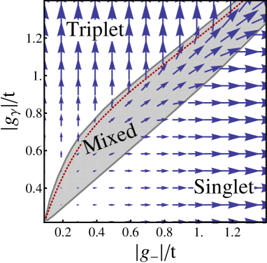
Figure 1: (Color online) Mean-field phase diagram characterizing singlet, triplet and mixed pairing states under time-reversal and $SU(2)$ symmetries (when the three triplet couplings are equal, $g_{\uparrow}=g_{\downarrow}=g_{+}\equiv g_{\gamma}$). The diagram is obtained by numerically solving the gap equations, which determine the equilibrium state of the system. Singlet ($|\Delta_{-}|$) and triplet ($|\Delta_{t}|$) pairing strengths are illustrated by vector arrows $(|\Delta_{-}|,|\Delta_{t}|)$ as a function of attractive singlet and triplet pair couplings, $g_{-}$ and $g_{\gamma}$, respectively (notice that both couplings are negative). Each arrow has length proportional to $\sqrt{|\Delta_{-}|^{2}+|\Delta_{t}|^{2}}$ and slope equal to $|\Delta_{-}/\Delta_{t}|$. Purely triplet and purely singlet regions (filled with horizontal and vertical arrows, respectively) sandwich a relatively narrow mixed-pairing region (shadowed, filled with finite-slope arrows), with boundaries marked by gray solid lines. The red dashed line in the mixed region indicates the boundary between topologically trivial (below) and nontrivial (above) regions as the chemical potential $\mu=-1.7t$. There is no pairing beyond the left and bottom axes of this diagram.

Numerically solving the gap equations in Eqs. (26) and (27) gives us the equilibrium state of the system. We obtain a mixed pairing state (where $|\Delta_{-}|\neq 0,|\Delta_{t}|\neq 0$) only in a restrictive region in the parameter space of negative (attractive) $g_{\gamma}$ and $g_{-}$. Outside this region there is no mixed-pairing solution, which means one or both of the gaps have to be zero. We thus solve Eq. (26) [Eq. (27)] for $|\Delta_{t}|$ ($|\Delta_{-}|$) by setting $|\Delta_{-}|=0$ ($|\Delta_{t}|=0$) in the triplet (singlet) coupling dominant region $|g_{\gamma}|>|g_{-}|$ ($|g_{-}|>|g_{\gamma}|$). In Fig. 1 we plot a phase diagram in the $|g_{-}|$-$|g_{\gamma}|$ plane for a low-filling case of $\mu=-1.7t$ and draw a boundary (red dashed curve) between topologically trivial and nontrivial regions. We use vector arrows $(|\Delta_{-}|,|\Delta_{t}|)$ to represent singlet and triplet pairing strengths, such that an arrow’s length is proportional to $\sqrt{|\Delta_{-}|^{2}+|\Delta_{t}|^{2}}$ and its slope is equal to $|\Delta_{-}/\Delta_{t}|$. We see that the vector length increases with the coupling strength. Horizontal and vertical arrows indicate purely singlet and triplet pairing phases, respectively, which sandwich a relatively narrow mixed-pairing region of finite-slope arrows. There is no pairing in regions of $|g_{-}|<0.1t$, $|g_{\gamma}|<0.2t$, or repulsive couplings. The diagram agrees with the picture of energetic competition between different pair species discussed in Sec. II; one can imagine $g_{-}$ and $g_{\gamma}$ as two “forces” that competitively stretch and orient the vectors. Our data show that the arrow smoothly rotates along a path from a singlet state to a triplet one across the mixed region, implying a continuous evolution of the system’s free energy.

When $SU(2)$ symmetry is broken ($g_{+}\neq g_{\uparrow}=g_{\downarrow}$), the pairings $\Delta_{+}$ and $\Delta_{\uparrow,\downarrow}$ are competing. Some pairings must vanish to obey Eqs. (LABEL:up_gap)–(LABEL:plus_gap_equation). Determining the vanishing pairings involves the comparison of the free energy corresponding to each pairing order. The one with higher free energy should vanish. However, computing the free energy is quite difficult. Instead, we give a qualitative argument as we did in Sec. II. The negative values of the coupling constants represent attractive interaction between the electrons. From the energetic point of view, stronger attractive force implies a higher possibility of pairing. Therefore, the pairing with stronger attractive coupling wins the competition. We can conclude that when $0\geq g_{+}>g_{\uparrow,\downarrow}$ ($0\geq g_{\uparrow,\downarrow}>g_{+}$), $\Delta_{+}=0$ ($\Delta_{\uparrow,\downarrow}=0$) and the pairings $\Delta_{\uparrow,\downarrow}$ ($\Delta_{+}$) dominate. In this case, Eqs. (LABEL:up_gap)–(LABEL:plus_gap_equation) becomes Eqs. (26) and (27) with $g_{\gamma}=g_{\uparrow,\downarrow}$ ($g_{+}$). As a result, the survival pairings are also determined by Eqs. (26) and (27) and hence described by Fig. 1.

From the mean-field approach, the coupling constants control singlet and triplet pairings. In the next section, we will study the exact ground state of a fixed-number open-end chain and compare the pairing behaviors with those in this section.

IV Exact solutions of a fixed-number open-end system

In this section we perform exact diagonalization using the Lanczos algorithmLin90 ; Dagotto94 to solve the Hamiltonian of an open-end chain with $L$ sites as well as fixed $N$ particles and discuss the pairing physics showed by the results. The exact solutions preserve all symmetries of the system and incorporate effects of quantum fluctuations that are ignored in the mean-field treatment. The $U(1)$ symmetry makes the Hamiltonian of Eq. (2) block-diagonalized with respect to the total number of each spin species ($N_{\uparrow}$ and $N_{\downarrow}$, as discussed in Sec. II) and hence allows us to deal with only the block where the ground state locates. However, this symmetry makes the original BCS-type pairing amplitude $\langle\hat{b}_{\alpha}\rangle$ no longer a good order parameter for the exact ground state.

Here we consider the pairing phenomenon as the condensation of paired fermionsYang62 ; Leggett06 . To study this, one can make an analogy to the condensation of bosons. In the Bose system, a condensed state can be identified by macroscopic occupation of a single-particle state, or mathematically, a macroscopic eigenvalue of the single-particle density matrixPenrose56 ; Leggett06 . In our Fermi system, it is the pair density matrix that is used to identify the pairing as a trend toward the macroscopic occupation of paired fermions. Specifically, we study the pairing tendency (favor or disfavor of pairing) by comparing the largest eigenvalue of the pair density matrix of the system with that of a free system. The pair density matrix ${\rho^{{\rm{pair}}}}$ is defined as

$$\rho_{{r_{1}}{\sigma_{1}},{r_{2}}{\sigma_{2}};{{r}_{1}^{\prime}}{{\sigma}_{1}^{\prime}},{{r}_{2}^{\prime}}{{\sigma}_{2}^{\prime}}}^{{\rm{pair}}}=\left\langle{\hat{c}_{{\sigma_{1}}{r_{1}}}^{\dagger}\hat{c}_{{\sigma_{2}}{r_{2}}}^{\dagger}{{\hat{c}}_{{{\sigma}_{2}^{\prime}}{{r}_{2}^{\prime}}}}{{\hat{c}}_{{{\sigma}_{1}^{\prime}}{{r}_{1}^{\prime}}}}}\right\rangle,$$ (29)

where the matrix indices are denoted by a set of two-particle states $\{{r_{1}}{\sigma_{1}},{r_{2}}{\sigma_{2}}\}$ with $r$ and $\sigma$ being spatial and spin quantum numbers, respectively. We compute the eigen functions of ${\rho^{{\rm{pair}}}}$ and find that each of them is also an eigen state of a pair’s total spin ${\hat{\bf S}^{{\rm{pair}}}}$ and its $z$ component $\hat{S}_{z}^{{\rm{pair}}}$. Therefore, each eigen function falls into one of the four pair classes including two intraspin triplet states for $\uparrow/\downarrow$ ($\{{S^{{\rm{pair}}}},S_{z}^{{\rm{pair}}}\}=\{1,\pm 1\}$), one interspin triplet state ($\{1,0\}$), and one singlet state ($\{0,0\}$). From each class we find the largest eigen value $\lambda^{(0)}$ and define a relative pair fraction as

$${P_{\alpha}}=\frac{{\lambda_{\alpha}^{(0)}-2}}{N},$$ (30)

where $\alpha=\uparrow,\downarrow,\pm$ denote the type of pairs in the same convention as in Sec. II and $N=N_{\uparrow}+N_{\downarrow}$ is the total number of particles. The relative pair fraction $P_{\alpha}$ is evaluated as a comparison with a free system, whose maximum eigenvalue is always 2 pairinfreesystem . Since a free system has no pairing preference, compared with this, positive (negative) $P_{\alpha}$ indicates the favor (disfavor) of $\alpha$ pair species. In the thermodynamic limit, the onset of pair condensation is signaled by $P\approx\lambda^{(0)}\sim O(1)$, although in most realistic systems $P=0.01\%$–$1\%$Leggett06 . In our case of an open chain, we take $P$ (i) positive, (ii) increasing as the system expands (by enlarging $L$ at fixed $N/L$), and (iii) increasing as the system dilutes (by enlarging $L$ at fixed $N$) as three signatures to identify a stable pairing state. Signature (ii) helps confirm the pairing tendency in the thermodynamic limit (see the applications on the Richardson modelRoman02 ; Dukelsky04 and the original Hubbard model discussed in Appendixes A and C, respectively), while (iii) does in the dilute regime of our interest (see discussions in Sec. IV.2 and Appendix C). Strictly speaking, such stable pairing state of a finite-size chain is not physically equivalent to a pair condensate that should be defined in the thermodynamic limit but could imply one if the trend persists. According to a theorem in Ref. [Yang62, ], the eigenvalues of a finite system with $N$ fermions and $L$ sites are bounded as $\lambda^{(0)}\leq N(2L-N+2)/2L$. Substituting a typical set in our calculations, $L=20$ and $N=8$, we obtain $P\leq 60\%$.

In the following we focus on the time-reversal symmetric case, so the number of independent couplings and hence that of independent pair species is reduced by 1, allowing us to denote $g_{\uparrow}=g_{\downarrow}\equiv g_{\updownarrow}$ and $P_{\uparrow}=P_{\downarrow}\equiv P_{\updownarrow}$. In Sec. IV.1 we discuss the finite-size effects and the stability of pairing in the dilute limit. We suggest a modification to maintain sufficient pairing tendency against the finite-size effects without the lost of generality. In Sec. IV.2, we present results showing the evolution of the system between different pairing states and the competition between these pairings. We plot state diagrams characterizing various stable pairing states as a function of couplings and compare them with the mean-field results obtained in Sec. III.

IV.1 Finite-size effects and stability of pairing

In a continuum system, only states within an energy scale of the pairing gap around the Fermi level mainly participate in Cooper pairing. In a finite-size chain of $L$ sites, the single particle spectrum is always discrete and gapped by $O(t/L)$. At a weak coupling of $|g_{\alpha}|<t/L$, it is the two degenerate states of spin up and down at the Fermi level that mainly participate in the interspin pairing, while the intraspin pairing is expected to be more suppressed due to the lack of two such available states. In fact, we explore the Hamiltonian of Eq. (2) with $N_{\uparrow,\downarrow}=4,L=8\sim 24$ and find that $P_{\pm}>0$ in a wide parameter range but $P_{\updownarrow}$ is always negative, even in the range of $g_{\updownarrow}<0,|g_{\updownarrow}|\simeq t\gg t/L$. In order to enhance the intraspin pairing, we increase the single particle density of states around the Fermi level by incorporating a second-nearest-neighbor tunneling into Eq. (2),

$$\sum\limits_{i}{\sum\limits_{\sigma=\uparrow,\downarrow}{-t^{\prime}\left({\hat{c}_{\sigma i}^{\dagger}{{\hat{c}}_{\sigma i+2}}+{\rm{H}}{\rm{.c}}{\rm{.}}}\right)}}.$$ (31)

In Fig. 2(a) we plot $P_{\updownarrow}$ (blue solid curve) and the single-particle density of state at the Fermi level (DoS, red dashed curve) as a function of the second nearest-neighbor tunneling strength $t^{\prime}$ for the case of an attractive $g_{\updownarrow}=-0.1t$, $g_{\pm}=0$, $N_{\uparrow}=N_{\downarrow}=4$, and $L=20$. We see that both $P_{\updownarrow}$ and DoS increase as $t^{\prime}$ increases from zero, simultaneously reaching the maxima around $t^{\prime}=-0.3t$. Such a trend agrees with our expectation that the more states are around the Fermi level, the higher pairing tendency the system shows. Below we consider a combined Hamiltonian of Eqs. (2) and (31) with $t^{\prime}=-t/3$ so $P_{\updownarrow}$ is large and positive ($\gg 0.01\%$) in a sufficiently large parameter regime. Notice that we implement $t^{\prime}$ to compensate the discreteness of states due to the finite-size effects. In a large enough system, we expect DoS around the Fermi level high enough for significant pairing even with only the nearest-neighbor tunneling as in Eq. (2).

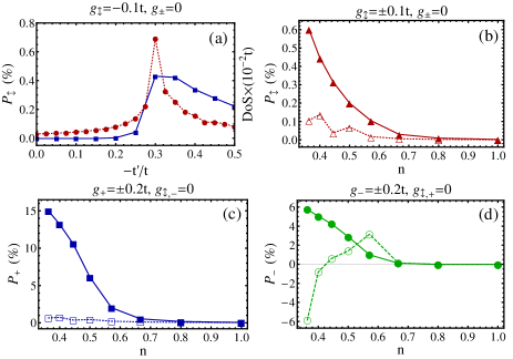
Figure 2: (Color online) (a) Intraspin pair fraction $P_{\updownarrow}$ (solid curve, axis on the left of graph) and the single-particle density of states (DoS) at the Fermi level (dashed curve, axis on the right of graph) vs the second-nearest-neighbor tunneling $t^{\prime}$. (b) Intraspin pair fraction $P_{\updownarrow}$ vs filling $n$ at attractive ($g_{\updownarrow}=-0.1t$, solid curve) and repulsive ($0.1t$, dashed) pairing interactions while the other two couplings are set zero, $g_{\pm}=0$. (c),(d) Interspin triplet and singlet pair fractions $P_{\pm}$ vs $n$ in attractive ($g_{\pm}=-0.2t$, respectively, solid curves) and repulsive ($0.2t$, dashed) cases, with the other two couplings set to zero as denoted in the plots. The relative pair fraction is measured from that of a free system, so negative values mean the disfavor of pairing.

Now we turn to discuss the stability of pairing in the low-filling regime of our interests. In the mean-field treatment in Sec. III, the pairing order vanishes if the corresponding coupling is positive (repulsive). In an open chain, we find that the relative pair fraction can be (slightly) positive in the repulsive regime. We attribute this to a finite-size effect and expect that attraction instead of repulsion is the relevant coupling for stable pairing as the system approaches the low-filling limit via expansion in size. Figures 2(b)–2(d) show the three relative pair fractions $P_{\updownarrow,+,-}$ as a function of filling number $n=(N_{\uparrow}+N_{\downarrow})/L$ at the corresponding coupling been attractive (solid curves) or repulsive (dashed ones), respectively. In each panel, we set the corresponding repulsive (attractive) interaction as $g_{\updownarrow,+,-}>0$ ($<0$) and keep the other two pairing effects irrelevant by setting the couplings to zero. The filling is varied by the tuning of $L$ at fixed $N_{\uparrow}=N_{\downarrow}=4$. We see that the pairing tendencies are inapparent at half filling ($n=1$) in all cases. Away from it, all the attractive cases show a monotonically increasing $P$ toward lower fillings, while in the repulsive cases $P$ either alternates in small positive values or becomes negative in the low-filling regime. We confirm two of the stable-pairing-state signatures discussed at the beginning of Sec. IV as (i) $P$ positive and (ii) monotonically increasing toward lower filling. Therefore, only the attractive interactions sustain a stable pairing state, in agreement with the mean field results in Sec. III. In Sec. IV.2 we use these two plus (iii) the increase of the pair fraction upon the system’s expansion at fixed filling to identify the stable pairing states and study the tuning between them in a general case in which more than one coupling is nonzero.

IV.2 Results and discussions

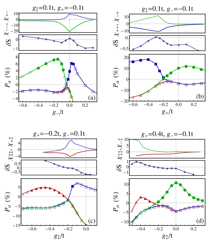
Figure 3: (Color online) Four cases shows relative pair fractions $P_{\alpha}$ (bottom panels), entanglement entropy $\delta S$ (middle) and pair susceptibility $\chi$ (top) tuned with the pairing couplings $g$. The intraspin, interspin triplet, and singlet pair fractions ($P_{\alpha=\updownarrow,+,-}$) are represented by red triangles, blue squares, and green circles, respectively. The filled (empty) symbols denote states that show (do not show) the three signatures for a stable pairing state discussed in text. (a) Tuning between singlet and interspin triplet pairings as the singlet coupling $g_{-}$ varies, while the top panel shows pair susceptibilities $\chi_{--}$ (green solid curve) and $\chi_{+-}$ (blue dashed). (b) Tuning between interspin triplet and singlet pairings as the interspin triplet coupling $g_{+}$ varies, presented together with $\chi_{++}$ (blue solid) and $\chi_{-+}$ (green dashed). (c) Tuning between intraspin and interspin triplet pairings as the intraspin coupling $g_{\updownarrow}$ varies, presented together with $\chi_{\updownarrow\updownarrow}$ (red solid) and $\chi_{+\updownarrow}$ (blue dashed). (d) Tuning between intraspin and singlet pairings as the intraspin coupling $g_{\updownarrow}$ varies, presented together with $\chi_{\updownarrow\updownarrow}$ (red solid) and $\chi_{-\updownarrow}$ (green dashed).

In this section, by computing the exact ground state of a time-reversal symmetric open-end chain with $N=8$ and $L=20$ (thus $N_{\uparrow}=N_{\downarrow}=4$ and the filling $N/L=0.4$) in a sufficiently wide parameter range of $g_{\updownarrow,+,-}$, we present results that show the evolution between different pairing states and thus identify paths of tuning between singlet and triplet or between multiple triplet pairing states in the parameter space. We also obtain state diagrams characterizing the stable regions for different pairing states. Following the three signatures discussed at the beginning of Sec. IV, a stable pairing state of pair species $\alpha$ here is identified by the relative pair fraction $P_{\alpha}$ (i) being positive, (ii) increasing as compared with cases of $L=18$ and $L=16$ at fixed $N=8$, and (iii) increasing as compared with that of $L=10$ at fixed $N/L=0.4$. In addition, we calculate two other physical quantities, pair susceptibility and von Neumann entanglement entropy, and study their behaviors upon the cross between two different stable-pairing regions. The pair susceptibility $\chi_{\alpha\beta}$ is defined as a second derivative of the ground-state energy $E_{G}$ with respect to the pairing couplings $g_{\alpha}$ and $g_{\beta}$,

$${\chi_{\alpha\beta}}=\frac{{{\partial^{2}}{E_{G}}}}{{\partial{g_{\alpha}}\partial{g_{\beta}}}}\times t,$$ (32)

with a multiplication of tunneling $t$ that makes $\chi$ dimensionless. According to the Hellmann-Feynman theorem, the first derivative of $E_{G}$ with respect to $g_{\alpha}$, $\partial{E_{G}}/\partial{g_{\alpha}}=\left\langle{\partial H/\partial{g_{\alpha}}}\right\rangle$, is hence proportional to the total number of $\alpha$ pairs on nearest-neighbor sites. Thus $\chi_{\alpha\beta}$ describes the response of the total number of such $\alpha$ pairs to $g_{\beta}$ (or $\beta$ pairs to $g_{\alpha}$ since $\chi_{\alpha\beta}$=$\chi_{\beta\alpha}$). The von Neumann entanglement entropy presented here is a relative value measured from the free case (where all pairing couplings vanish),

$$\delta S=-{\rm{Tr}}\left({{\rho^{{\rm{red}}}}\ln{\rho^{{\rm{red}}}}-\rho_{0}^{{\rm{red}}}\ln\rho_{0}^{{\rm{red}}}}\right),$$ (33)

where ${{\rho^{{\rm{red}}}}}$ is a reduced density matrix constructed by tracing out the degrees of freedom of the right-half chain, and ${{\rho_{0}^{{\rm{red}}}}}$ is that of a free system. The relative entanglement entropy quantifies how much more or less entangled (positive or negative $\delta S$, respectively) the system is driven by the pairing couplings.

In Fig. 3, we plot $P_{\updownarrow,+,-}$ (red triangles, blue squares, and green circles, respectively) vs $g$ in four cases that show the tuning between different stable pairing states (filled symbols in the $P$ curve contract to the empty ones denoting states that do not satisfy the three stability criterions). The bottom panel of Fig. 3(a) shows the tuning between interspin triplet and singlet pairing states ($P_{+}$ and $P_{-}$ dominates, respectively) as we vary $g_{-}$ and keep $g_{\updownarrow}$ repulsive as well as $g_{+}$ attractive. We see that the intraspin triplet pairing is always unfavorable ($P_{\updownarrow}<0$ everywhere). The interspin triplet pairing is stable in a region of weakly positive and negative $g_{-}$, while the interspin singlet pair fraction rises, overcomes the interspin triplet one across a switch point where $P_{+}=P_{-}$, and becomes stable as $g_{-}$ goes more negative. Toward the region of largely positive (negative) $g_{-}$, the interspin triplet (singlet) pairing decreases and becomes unstable. In the bottom panel of (b), we plot the tuning between the same two pairing states but in a different path in which $g_{+}$ is varied and $g_{-}$ is kept attractive. We see a similar competition that the singlet pairing dominates until is conquered by the interspin triplet one as $g_{+}$ goes sufficiently negative. The bottom panel of (c) [(d)] shows how the stable intraspin triplet pairing state emerges with the suppression of interspin triplet (singlet) pairing as $g_{\updownarrow}$ varies from positive toward sufficiently negative regions. In general, we find the tunability from stable $\beta$-pairing to $\alpha$-pairing states, across a switch point where $P_{\alpha}=P_{\beta}$, by varying $g_{\alpha}$ from positive to sufficiently negative values and keeping $g_{\beta}$ a negative constant, also in a condition that the other coupling $g_{\gamma}$ is set positive for the disfavor of $\gamma$ pairing all the time. Both facts of (1) the switch between stable $\beta$- and $\alpha$-pairing states around a negative $g_{\alpha}$ and (2) increasing $P_{\alpha}$ accompanied with decreasing $P_{\beta}$ around the switch point indicate a competition between the two pair species: $g_{\alpha}$ has to overwhelm $g_{\beta}$ to make the $\alpha$-pair species dominant. This results agrees with the phenomenological discussions in Sec. II using the number-conserving BCS ansatz of Eq. (8). The competition also implies that a mixed state of two stable pairings either hardly occurs or does so in a relatively small parameter range. In fact, only in (b) do we see a mixture of weakly stable interspin triplet and singlet pairings ($P\gtrsim 0$) around a small region of $g_{+}=-0.2t$, while the other three cases lack such mixture. We will discuss the mixed pairing state in more details later.

Here we turn to study the pair susceptibility $\chi$, which could show more information about the competition. The top panels of (a)–(d), cases with tuning $g_{\alpha}$ at negatively constant $g_{\beta}$, show $\chi_{\alpha\alpha}$ and $\chi_{\beta\alpha}$ (or the rate of change in numbers of nearest-neighbor $\alpha$ and $\beta$ pairs with $g_{\alpha}$) vs $g_{\alpha}$ (solid and dashed curves, respectively). We see in (a)–(c) that both $\chi_{\alpha\alpha}$ and $\chi_{\beta\alpha}$ develop peaks with opposite signs around the switch point where $P_{\alpha}=P_{\beta}$, reflecting a drastic increase of $\beta$ pairs and drop of $\alpha$ pairs as $g_{\alpha}$ increases toward the positive or repulsive region. The slight mismatch between the switch point and the susceptibility peaks can be due to the difference between $P$ and $\chi$; the former represents pairs only for the dominant eigen wavefunction of the pair density matrix, while the latter counts the nearest-neighbor pairs only. In (d), neither $\chi_{\updownarrow\updownarrow}$ nor $\chi_{-\updownarrow}$ exhibits a peak around the switch point $g_{\updownarrow}=-0.23t$. This shows that the competition between intraspin triplet and interspin singlet pairings is much weaker than that between any other sets of two pairings. In addition, we plot the relative entanglement entropy $\delta S$ vs $g$ on each of the middle panel of (a)–(d). We see in most stable pairing regions in (a) and (b) that the interspin triplet and singlet pairing states are less entangled than the free system, or $\delta S<0$, while it reaches a local maximum (slightly positive) around the switch point and the peak of $\chi$. In the stable pairing regions in (c) and (d), $\delta S$ monotonically decreases from positive to negative as $g_{\updownarrow}$ increases, with its zero value exactly on the switch point. These results show that the intraspin pairing state tends to sustain higher long-range entanglement than the free system, while the two interspin pairing ones do the opposite.

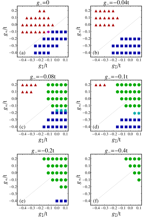
Figure 4: (Color online) (a)–(f)State diagrams showing stable pairing regions in $g_{+}$-$g_{\updownarrow}$ plane at $g_{-}/t=0$, $-0.04$, $-0.08$, $-0.1$, $-0.2$, and $-0.4$, respectively. Red triangles, blue squares and green circles represent intraspin, interspin triplet and singlet pairing, respectively, while the magenta diamonds and cyan stars represent a mix of intraspin and interspin pairings as well as that of interspin triplet and singlet pairings, respectively. The dashed lines $g_{+}=g_{\updownarrow}$ indicates $SU(2)$ symmetry of the system.

In Fig. 4, we plot state diagrams characterizing regions of various stable paring states, including intraspin triplet (denoted by triangles), interspin triplet (squares), and singlet pairings (circles), as well as a mixture of the two triplet pairings (diamonds) and that of the interspin triplet and singlet pairings (stars), in the $g_{\updownarrow}$–$g_{+}$ plane at a descending series of $g_{-}/t=0$, $-0.04$, $-0.08$, $-0.1$, $-0.2$ and $-0.4$ [(a)–(f), respectively]. The dashed line on each diagram denotes the $SU(2)$-symmetric region where $g_{+}=g_{\updownarrow}$. At $g_{-}=0$ [(a)], the diagram has stable intraspin and interspin triplet pairing regions, which qualitatively match $\{g_{\updownarrow}<0,g_{+}>g_{\updownarrow}\}$ and $\{g_{+}<0,g_{+}<g_{\updownarrow}\}$, respectively, indicating the survival pairing state due to both the attractive interaction and the success in competition against the other one. There is no stable pairing state in a region where the two couplings are both repulsive or both strongly attractive such that no one wins the competition. The diagram also shows no stable singlet pairing everywhere. Remarkably, we find a mixed pairing state with both triplet pairings being stable on the overlap between the two triplet pairing regions along the dashed line denoting $SU(2)$ symmetry. We check that the mixed state has the same pair fractions of the two triplet pairings $P_{\updownarrow}=P_{+}$, in agreement with the discussion in Sec. II that this mixture is guaranteed by $SU(2)$ symmetry. [In fact, all data points along the dashed lines in Fig. 4 show the same set of eigenvalues corresponding to the intraspin and interspin triplet pairings, $\{\lambda^{(i)}_{\updownarrow}\}=\{\lambda^{(i)}_{+}\}$, reflecting the $SU(2)$ symmetry of the pair density matrix (see details in Appendix D).] At $g_{-}=-0.04t$ [(b)], the two triplet pairing regions separately move away from the dashed line, no longer overlap, and hence leave no mixed pairing state. At $g_{-}=-0.08t$ [(c)], the two triplet pairing regions further separate and there appear singlet pairing states in the region of positive or slightly negative $g_{\updownarrow,+}$. The singlet pairing region overlaps the intraspin triplet one, producing a mixed pairing region on a horizontal line of $\{g_{+}=-0.16t=2g_{-},g_{\updownarrow}\geq 0\}$. This mixture comprises triplet and singlet pair species, which have different total spin angular momentum but the same $\hat{z}$-component one. Since there is no symmetry protection here, the pair fractions of both species are not necessarily equal, or in general, $P_{+}\neq P_{-}$. At $g_{-}=-0.1t$ [(d)], the state diagram is similar to (c), with further withdrawals of intraspin and interspin triplet pairing regions toward the top-left and bottom-right corners, respectively, an expansion of singlet pairing region, and a shift of the mixed region of interspin triplet and singlet pairings to a horizontal line of $\{g_{+}=-0.2t=2g_{-},g_{\updownarrow}\geq 0.05t\}$. At $g_{-}=-0.2t$ [(e)], the intraspin triplet pairing disappears in the parameter range of interests, while the interspin triplet and singlet pairing regions further separate from each other such that the mixed region disappears as well. Finally, at a relatively strong $g_{-}=-0.4t$ [(f)], only a small singlet pairing region survives in the scope, occupying the top-right corner of the diagram.

We turn to compare the mean-field results for a translation-invariant system obtained in Sec. III and the exact solutions for a fixed-number open-end chain here. First, both cases show that a pairing state exists only if the corresponding pairing coupling is attractive (negative). If two or more pairing couplings are attractive, the corresponding pairing states will compete with each other. Second, the quantities that characterize pairing (the gaps in Sec. III or the pair fractions here) always satisfy the same time-reversal or $SU(2)$ symmetry or both as the Hamiltonian does. Given time-reversal symmetry, both cases can show mixed-pairing solutions of singlet and triplet pairings. Given both time-reversal and $SU(2)$ symmetries, the mean-field case still shows this mixture but the open-chain case does not. In addition, the open-chain case does not exhibit notable topological signatures as the BdG Hamiltonian does in the mean-field case. We attribute these issues to the finite-size effects in the open-chain case and expect the two cases’ results closer to each other as the open-end chain size increases. To achieve this, the study using density matrix renormalization-group methodsWhite93 ; Schollwock05 would be helpful.

V Conclusion

In this paper, we studied a low-filling Hubbard chain model with nearest-neighbor charge and spin interactions, which produce four independently tunable pairing couplings, corresponding to two intrapin triplet, one interspin triplet, and one singlet pairing channels, respectively. First, we performed a mean-field treatment on a large-size system with translational invariance and derived four gap equations characterizing the pairing order parameters. The BdG Hamiltonian obtained in the treatment can exhibit nontrivial topology in a chemical potential range that is the same as Kitaev’s modelKitaev01 in a purely triplet pairing state but shrinks with the presence of a singlet pairing order. The mean-field phase diagram under the time-reversal and $SU(2)$ symmetries shows a purely triplet or singlet pairing region if the corresponding coupling overwhelms the other and a mixed pairing region when both couplings are compatible. (After the completion of this work, we perceived that two other works investigating two-dimensional electronic systems also indicated a topological phase transition due to the competition between triplet and singlet pairing states.Lu13 ; Yao13 ) Second, we employed an exact-diagonalization algorithm to compute the many-body ground state of an open-end fixed-number system with modification to reduce the finite-size effect. We used three signatures of pair fractions to identify a stable pairing state of the system, which approaches a pair condensate if such trends persist. Our results under the time-reversal symmetry show a stable intraspin triplet, interspin triplet, or singlet pairing state in a region where the corresponding coupling dominates and an overlapped region of mixed intraspin and interspin triplet or mixed interspin triplet and singlet pairing states. The system’s switch from the singlet or intraspin triplet pairing state to the interspin triplet one accompanies a peak in the pair susceptibility, and that from the singlet or interspin triplet pairing state to the intraspin triplet one accompanies a sign change in the relative entanglement entropy. Both the mean-field and exact-diagonalization cases agreeably show a competitive nature of these pairings and hence enable the tuning of the system between different pairing states as well as mixtures of them.

Finally, we point out two platforms with properties suited for the potential realization of tunable pairing channels—the key mechanism in our model. First, recently focused Rydberg or Rydberg-dressed atomic gasesHenkel10 ; *Pupillo10; *Saffman10; *Honer10; *Mukherjee11; *Schmidt-Kaler11; *Sevincli11; *Ji11; *Schaub12; *Viteau12; *Hague12; *Lauer12; *Robert-de-Saint-Vincent13; *Baluktsian13; *Mattioli13; *McQuillen13; *Honing13 exhibit controllable $s$-wave and $p$-wave two-body interactionsHamilton02 ; Kurz13 as well as significant nearest-neighbor couplings when loaded in optical latticesPohl10 ; Weimer10 ; Viteau11 ; Anderson11 ; Saha14 . Second, multispecies dipolar gasesSamokhin06 ; *Wu10; *Shi10; *LiaoR10; *Kain11; *Shi13; *Qi13 have been investigated for the competition between short-range singlet and long-range triplet interactions, capable of realizing various pairing states and their mixture in higher-dimensional systems. In addition, a recent experimentGreif13 has demonstrated a method to measure the spin-correlation in optical lattices, which is directly related to the pair fraction in our study. However, how to tailor theses ideas to a practical scheme for our chain lattices is a challenge. One of the future directions is to study the model realization and to propose experimental detection for its pairing order as well as topological state.

Appendix A Validity of mean-field and exact-diagonalization calculations on the Richardson model

In this Appendix, we perform mean-field (MF) and exact-diagonalization (ED) calculations on the Richardson modelRoman02 ; Dukelsky04 , which is a 1D exactly solvable model approaching the BCS limit. Our results show the critical coupling for the onset of superconductivity consistent with the exact solution and thus the validity of both methods on 1D superconducting systems (such as our model) to a certain extent.

For both $U(1)$-preserving finite-size and $U(1)$-breaking infinite-size systems, computing the pair density matrix of Eq. (29) is a valid method to determine the presence of superconducting pairingLeggett06 . A macroscopic eigenvalue of the pair density matrix shows the region of coupling constant corresponding to a pair condensation or the superconducting pairing. In the following, we calculate the pair density matrix by performing ED on a few-body finite-size Richardson model and MF treatment on the model in the thermodynamic limit. The Richardson model is described by a half filling Hamiltonian in the form of

$$H_{\rm{R}}=\frac{2}{1}\sum_{j=1,\sigma=\uparrow,\downarrow}^{N}{\epsilon_{j\sigma}}c^{\dagger}_{j\sigma}c_{j\sigma}-G\sum_{j,j^{\prime}=1}^{N}c^{\dagger}_{j\uparrow}c^{\dagger}_{j\downarrow}c_{j^{\prime}\downarrow}c_{j^{\prime}\uparrow},$$

where $N$ denotes the number of sites, which is equal to the number of particles, and $G$ is the coupling constant. The Hamiltonian is different from the BCSBardeen57 Hamiltonian in lattices. The single-body term describes an on-site energy ($\epsilon_{j\sigma}$) instead of hopping, and the two-body term represents interaction within all possible ranges rather than the on-site one. The Hamiltonian above still preserves $U(1)$ symmetry and can be exactly solved to obtain the many-body ground state and the ground-state energy. By choosing some specific energy $(\epsilon_{j\sigma})$ distribution, the physical phase of the system can be determined in the thermodynamic limit ($N\rightarrow\infty$). In the following, we discuss the onset of superconductivity in a two-level distribution $\epsilon_{j\sigma}=\pm\epsilon_{1}$. For the comparison between different system sizes, we normalize the interacting effects by defining a normalized coupling constant $g=GN$. We note that the arrangement of the energies on each site does not change the physical properties because the strength of the interaction in each range is described by the same coupling constant $G$.

By performing ED, we obtain the pair density matrices for the ground states of $N=6$, $8$, and $10$. The presence of the superconducting pairing is determined by the largest eigenvalue of the pair density matrix being $O(N)$. In our ED case, the system size is always too small to make a conclusion. Instead, we calculate the relative pair fraction $P_{N}$ for $N$ particles as defined in Eq. (30) but only for the singlet pairing here (so the spin index $\alpha$ is dropped for convenience). The $-2$ in the definition of $P$ is to measure the eigenvalue from that of a free systempairinfreesystem (also see detailed discussions in Sec. IV). If the superconducting pairing occurs, we expect that $P$ increases as $N$ increases, which suggests that $P_{N}-P_{N-2}$ changes sign across the transition point. As shown in the inset of Fig. 5, at $N=10$ the transition point is near $g=-1$ and $P_{N}>P_{N-2}$ as $g<-1$ so the region of $g<-1$ corresponds to possible superconductor pairing. Our result is consistent with the two-level Richardson model in the thermodynamic limit discussed in Ref. Roman02, .

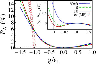
Figure 5: (Color online) The relative pair fraction $P_{N}$ vs normalized coupling constant $g$ at half-filling with three different particle numbers of $N=6$, $8$, and $10$ (blue dotted, green dashed, and red solid curves, respectively). In the region of $g/\epsilon_{1}<-1$, larger $N$ means larger $P_{N}$, so the system is regarded as a superconducting state. The inset shows that the phase-transition point $P_{N}-P_{N-2}=0$ approaches the exact solution $g_{c}=-\epsilon_{1}$ as $N$ increases. The red circles, which are for an infinitely large-size system predicted by the mean-field (MF) treatment, show that $P$ rises from zero exactly at $g_{c}$.

In the following, we use a MF treatment to calculate the pair fraction in the thermodynamic limit ($N\to\infty$) and compare it with the results from ED as well as the exact solution. The order parameter is defined as a function of spacial coordination $\Delta_{i}=\sum_{j}(-G_{ij})\left<c_{j\downarrow}c_{j\uparrow}\right>$ (where the coupling $G_{ij}$ is first assumed spatial dependent). At the MF level, the Hamiltonian can be rewritten as

$$H^{\rm MF}_{\rm R} = \sum_{i}\left(c^{\dagger}_{i\uparrow},c_{i\downarrow}\right)H_{i}\left(\begin{array}[]{c}c_{i\uparrow}\\ c^{\dagger}_{i\downarrow}\end{array}\right)-\sum_{ij}(G^{-1})_{ij}\Delta^{*}_{i}\Delta_{j},$$ (37)

$$H_{i} = \left(\begin{array}[]{cc}\frac{1}{2}(\epsilon_{i\uparrow}-\mu)&\Delta^{*}_{i}\\ \Delta_{i}&-\frac{1}{2}(\epsilon_{i\downarrow}-\mu)\end{array}\right).$$ (40)

The energy and the corresponding eigenstates are the followings,

$$E_{\pm} = \mu_{i}\pm E_{i},$$ (41)

$$\mu_{i} = \frac{1}{4}\left(\epsilon_{j\uparrow}-\epsilon_{j\downarrow}\right),$$ (42)

$$E_{i} = \sqrt{\frac{1}{16}\left(\epsilon_{j\uparrow}+\epsilon_{j\downarrow}-2\mu\right)^{2}+|\Delta_{j}|^{2}}$$ (43)

$$\equiv \sqrt{\varepsilon_{i}^{2}+|\Delta_{i}|^{2}},$$

$$\Phi^{\dagger}_{i+}\left|{\psi_{g}}\right\rangle = \left(\cos\frac{\theta_{i}}{2}c^{\dagger}_{i\uparrow}+\sin\frac{\theta_{i}}{2}e^{i\phi_{i}}c_{i\downarrow}\right)\left|{\psi_{g}}\right\rangle$$ (44)

$$\equiv \left(u_{i}c^{\dagger}_{i\uparrow}+v_{i}c_{i\downarrow}\right)\left|{\psi_{g}}\right\rangle,$$

$$\Phi^{\dagger}_{i-}\left|{\psi_{g}}\right\rangle = \left(-\sin\frac{\theta_{i}}{2}c^{\dagger}_{i\uparrow}+\cos\frac{\theta_{i}}{2}e^{i\phi_{i}}c_{i\downarrow}\right)\left|{\psi_{g}}\right\rangle,$$ (45)

$$\tan\theta_{i} = \frac{|\Delta_{i}|}{\varepsilon_{i}},\tan\phi_{i}=\frac{\rm Im\Delta_{i}}{\rm Re\Delta_{i}}.$$ (46)

Here $\left|{{\psi_{g}}}\right\rangle$ is the ground state and $\Phi^{\dagger}_{i\pm}$ are quasiparticle operators. Similar to the BCS theory, we have the self-consistent gap equation as

$$\Delta_{i}=\sum_{j}(-G_{ij})\frac{\Delta_{j}}{2E_{j}}\left[\frac{1}{e^{\beta(\mu_{j}+E_{j})}+1}-\frac{1}{e^{\beta(\mu_{j}-E_{j})}+1}\right].$$

For simplicity, we consider the same setup as in the ED case, $\mu_{i}=0$ and $\varepsilon_{i}=\epsilon_{1}/2$. By assuming the homogeneity of the system, $\Delta_{i}=\Delta$, $G_{ij}=G$, and $E_{i}=E$, the gap equation becomes

$$|\Delta| = (-g)\frac{|\Delta|}{2E}\tanh\left(\frac{\beta E}{4}\right).$$ (48)

At zero temperature, the gap equation can be simplified as

$$|\Delta| = (-g)\frac{|\Delta|}{2E},$$ (49)

and results in a solution $|\Delta|=\sqrt{g^{2}-\epsilon_{1}^{2}}/2$. The transition from a normal phase ($\Delta=0$) to a superconducting phase ($\Delta\neq 0$) appears at a critical coupling $g_{c}=-\epsilon_{1}$ as $g$ goes below $g_{c}$. These results agree with the exact solution.

Now we turn to calculate the pair fraction. The MF ground state can be obtained as

$$\left|{{\psi_{g}}}\right\rangle=\prod\limits_{i}{\left({{u_{i}}c_{i\uparrow}^{\dagger}c_{i\downarrow}^{\dagger}+{v_{i}}}\right)}\left|{{\rm{vac}}}\right\rangle.$$ (50)

Then the pair density matrix is of the form

$$\rho_{{i_{1}}{\sigma_{1}},{i_{2}}{\sigma_{2}};{{i}_{1}^{\prime}}{{\sigma}_{1}^{\prime}},{{i}_{2}^{\prime}}{{\sigma}_{2}^{\prime}}}^{{\rm{pair}}}=\left\langle{\hat{c}_{{i_{1}}{\sigma_{1}}}^{\dagger}\hat{c}_{{i_{2}}{\sigma_{2}}}^{\dagger}{{\hat{c}}_{{{i}_{2}^{\prime}}{{\sigma}_{2}^{\prime}}}}{{\hat{c}}_{{{i}_{1}^{\prime}}{{\sigma}_{1}^{\prime}}}}}\right\rangle$$ (51)

$$= {\delta_{{i_{1}}{i_{2}}}}{\delta_{{{i}_{1}^{\prime}}{{i}_{2}^{\prime}}}}{\delta_{{\sigma_{1}},-{\sigma_{2}}}}{\delta_{{{\sigma}_{1}^{\prime}},-{{\sigma}_{2}^{\prime}}}}(\delta_{\sigma_{1},\uparrow}-\delta_{\sigma_{1},\downarrow})(\delta_{\sigma_{1}^{\prime},\uparrow}-\delta_{\sigma_{1}^{\prime},\downarrow})$$

$$\times \left[\delta_{i_{1},i_{1}^{\prime}}|u_{i_{1}}|^{2}+(1-\delta_{i_{1},i_{1}^{\prime}})u^{*}_{{i_{1}}}v^{*}_{{i_{1}^{\prime}}}u_{{i_{1}^{\prime}}}v_{{i_{1}}}\right]$$

$$+ (1-\delta_{i_{1},i_{2}})\left[{\delta_{{i_{1}}{i_{1}^{\prime}}}}{\delta_{{{i}_{2}}{{i}_{2}^{\prime}}}}{\delta_{{\sigma_{1}},{\sigma_{1}^{\prime}}}}{\delta_{{{\sigma}_{2}},{{\sigma}_{2}^{\prime}}}}\right.$$

$$- \left.\delta_{{i_{1}}{i_{2}^{\prime}}}{\delta_{{{i}_{2}}{{i}_{1}^{\prime}}}}{\delta_{{\sigma_{1}},{\sigma_{2}^{\prime}}}}{\delta_{{{\sigma}_{2}},{{\sigma}_{1}^{\prime}}}}\right].$$

In the uniform case, only the off-diagonal elements

$$\rho_{i\sigma,i(-\sigma);i^{\prime}\sigma,i^{\prime}(-\sigma)}^{{\rm{pair}}}=-\rho_{i\sigma,i(-\sigma);i^{\prime}(-\sigma),i^{\prime}\sigma}^{{\rm{pair}}}={\left|u\right|^{2}}{\left|v\right|^{2}}$$

($i\neq i^{\prime}$) contribute to the macroscopic eigenvalue $\lambda^{(0)}$ and hence the pair fraction $P$ in the large-$N$ limitPenrose56 ; Yang62 ; Leggett06 ; Sun09 . They are obtained as

$$\lambda^{(0)} \approx 2N{\left|u\right|^{2}}{\left|v\right|^{2}}=\frac{N}{2}\left[1-\left(\frac{\varepsilon}{E}\right)^{2}\right],$$ (53)

$$P = \frac{\lambda_{\rm max}-2}{N}\approx\frac{(g^{2}-\epsilon_{1}^{2})}{2g^{2}}.$$ (54)

The above equations work only for $g<0$ or attractive interaction. We can see that the pair fraction $P$ rises from zero when $g<g_{c}=-\epsilon_{1}$ (see red circles in Fig. 5), which means that the superconducting pairing appears as the attractive interaction becomes stronger than the critical value. This predicted $g_{c}=-1$ from the pair fraction agrees with our ED calculations. We also see a trend that the ED results approach the MF ones as $N$ increases.

Appendix B $\mathbb{Z}_{2}$ topological invariant in a class DIII chain

In this Appendix, we compute $\mathbb{Z}_{2}$ invariant for the BdG Hamiltonian $H_{p}^{\rm{BdG}}$ in Eq. (13), which can distinguish the topologically nontrivial and trivial phases more rigorously. To simplify the problem, let us first perform an $SU(2)$ transformation in spin basis

$$\begin{pmatrix}c^{\dagger}_{\uparrow}\\ c^{\dagger}_{\downarrow}\end{pmatrix}=\begin{pmatrix}\nu&\eta\\ -\eta^{*}&\nu^{*}\end{pmatrix}\begin{pmatrix}c^{\prime\dagger}_{\uparrow}\\ c^{\prime\dagger}_{\downarrow}\end{pmatrix}.$$ (55)

The unitarity of $SU(2)$ requires $|\nu|^{2}+|\eta|^{2}=1$. After the $SU(2)$ transformation, the pairing functions in $H^{\rm{BdG}}_{p}$ is given by

$$\Delta^{\prime}_{\uparrow} = \Delta_{\uparrow}\nu^{2}+\Delta_{\downarrow}\eta^{*2}+\sqrt{2}\Delta_{+}\nu\eta^{*},$$ (56)

$$\Delta^{\prime}_{\downarrow} = \Delta_{\uparrow}\eta^{2}+\Delta_{\downarrow}\nu^{*2}-\sqrt{2}\Delta_{+}\nu^{*}\eta,$$ (57)

$$\Delta^{\prime}_{+} = -\sqrt{2}\Delta_{\uparrow}\nu\eta+\sqrt{2}\Delta_{\downarrow}\nu^{*}\eta^{*}+\Delta_{+}(|\nu|^{2}-|\eta|^{2}),$$ (58)

$$\Delta^{\prime}_{-} = \Delta_{-}.$$ (59)

Therefore, $\Delta_{-}$ is invariant under $SU(2)$ due to the singlet pairing. Furthermore, we find $\Delta_{+}^{2}-2\Delta_{\uparrow}\Delta_{\downarrow}$ and $|\Delta_{t}|^{2}=|\Delta|^{2}+|\Delta_{\uparrow}|^{2}+|\Delta_{\downarrow}|^{2}$ also invariant under the $SU(2)$ transformation. We note that the time-reversal constraints for the pairings in Eq. (14) still hold under $SU(2)$ so $\Delta_{-}$ is real. By choosing a proper $SU(2)$ transformation, the three triplet pairings can be simplified as $\Delta_{\uparrow}=\Delta_{\downarrow}\equiv\Delta_{t}/\sqrt{2}$ is real and $\Delta_{+}$ vanishes. Therefore, the BdG Hamiltonian can be written as

$$H^{\rm{BdG}}_{p}=\begin{pmatrix}\frac{-2t\cos p-\mu}{2}&0&\frac{i\sin p\Delta_{t}}{\sqrt{2}}&-\frac{\cos p\Delta_{-}}{\sqrt{2}}\\ 0&\frac{-2t\cos p-\mu}{2}&\frac{\cos p\Delta_{-}}{\sqrt{2}}&\frac{i\sin p\Delta_{t}}{\sqrt{2}}\\ -\frac{i\sin p\Delta_{t}}{\sqrt{2}}&\frac{\cos p\Delta_{-}}{\sqrt{2}}&\frac{2t\cos p+\mu}{2}&0\\ -\frac{\cos p\Delta_{-}}{\sqrt{2}}&-\frac{i\sin p\Delta_{t}}{\sqrt{2}}&0&\frac{2t\cos p+\mu}{2}\end{pmatrix}.$$

After performing a unitary transformation

$$U=\frac{1}{2}\begin{pmatrix}i&-1&-i&1\\ 1&-i&1&-i\\ -i&1&-i&1\\ -1&i&1&-i\\ \end{pmatrix},$$ (61)

we can simplify the BdG Hamiltonian as

$$H^{\prime\rm{BdG}}_{p}=UH^{\rm{BdG}}_{p}U^{\dagger}$$ (62)

$$= \begin{pmatrix}0&0&A_{+}e^{-i\theta_{+}}&0\\ 0&0&0&A_{-}e^{-i\theta_{-}}\\ A_{+}e^{i\theta_{+}}&0&0&0\\ 0&A_{-}e^{i\theta_{-}}&0&0\\ \end{pmatrix},$$

where

$$A_{\pm}(p)e^{i\theta_{\pm}(p)}=\frac{2t\cos p+\mu}{2}+\frac{i}{\sqrt{2}}(\cos p\Delta_{-}\pm\sin p\Delta_{t}).$$

Similarly, the time-reversal operator under the unitary transformation becomes

$$\Theta^{\prime}=\begin{pmatrix}0&i\tau_{y}\\ i\tau_{y}&0\\ \end{pmatrix}K.$$ (64)

Solving the eigen problem in the half filling scenario, we have two occupied eigenstates with negative energies,

$$|u^{\rm{I}}(p)\rangle = \begin{pmatrix}e^{-i\theta_{+}(p)/2}&0&e^{i\theta_{+}(p)/2}&0\end{pmatrix}^{T},$$ (65)

$$|u^{\rm{II}}(p)\rangle = \begin{pmatrix}0&e^{-i\theta_{-}(p)/2}&0&e^{i\theta_{-}(p)/2}\end{pmatrix}^{T}.$$ (66)

Furthermore, these two states are time-reversal partners ($|u^{\rm{I}}(p)\rangle=\Theta^{\prime}|u^{\rm{II}}(-p)\rangle,\ |u^{\rm{II}}(p)\rangle=-\Theta^{\prime}|u^{\rm{I}}(-p)\rangle$).

Finally, we are able to compute the topological invariant from the occupied states. The definition of the $Z_{2}$ topological invariant in one dimension for symmetry class DIII is given byFu06 ; Budich13

$$P^{I}_{o}=\frac{1}{2\pi}\left[\int^{\pi}_{0}dp\mathcal{A}_{o}(p)+i\ln\left(\frac{\rm{Pf}\theta_{o}(\pi)}{\rm{Pf}\theta_{o}(0)}\right)\right],$$ (67)

where $\mathcal{A}_{o}(p)=-i(\langle u^{\rm{I}}(p)|\partial_{p}|u^{\rm{I}}(p)\rangle+\langle u^{\rm{II}}(p)|\partial_{p}|u^{\rm{II}}(p)\rangle)$, $\theta_{o}(p)$ is a matrix defined as $\theta_{o}^{\alpha\beta}(p)=\langle u^{\alpha}(p)|\Theta^{\prime}|u^{\beta}(-p)\rangle$ and Pf denotes the Pfaffian. When particle-hole symmetry is present, $P^{I}_{o}$ is quantized and its value (mod $1$) describes topology in 1D time-reversal superconductors (0 trivial and 1/2 nontrivial). In our case,

$$P^{I}_{o}=\frac{i}{2\pi}\ln\left(\frac{\cos(\frac{\theta_{-}(0)-\theta_{+}(0)}{2})}{\cos(\frac{\theta_{-}(\pi)-\theta_{+}(\pi)}{2})}\right),$$ (68)

where

$$\theta_{-}(0)-\theta_{+}(0) = 0,$$ (69)

$$\theta_{-}(\pi)-\theta_{+}(\pi) = \begin{cases}0,\quad\quad\rm{as}\ \frac{4\Delta_{t}^{2}t^{2}}{\Delta_{t}^{2}+\Delta_{-}^{2}}<\mu^{2},\\ -2\pi,\ \ \rm{as}\ \frac{4\Delta_{t}^{2}t^{2}}{\Delta_{t}^{2}+\Delta_{-}^{2}}>\mu^{2},\end{cases}$$ (70)

Therefore, when $\frac{4\Delta_{t}^{2}t^{2}}{\Delta_{t}^{2}+\Delta_{-}^{2}}>\mu^{2}$, $P^{I}_{o}=1/2$ corresponds to a topologically nontrivial phase, which is consistent with the topological region in Eq. (17) with $SU(2)$ invariant $\Delta_{-}$ and $\Delta_{t}^{2}$.

Appendix C Trends of the pair fraction in a Hubbard chain with onsite interaction

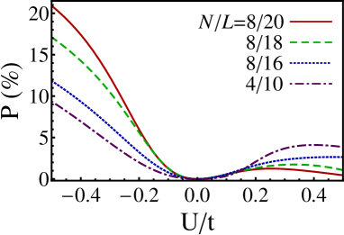
Figure 6: (Color online) The relative pair fraction $P$ vs on-site interaction $U$ in a Hubbard chain with various numbers of particles $N$ and sites $L$. The red solid, green dashed, blue dotted, and purple dot-dashed curves represent the cases of $(N,L)=(8,20)$, $(8,18)$, $(8,16)$, and $(4,10)$, respectively. In the attractive interaction region ($U<0$), increasing size at fixed $N$ (as the system dilutes) and at fixed $N/L$ (extends) coincides with positive and increasing $P$, so the system is regarded as a stable pairing state or a superconducting state in the thermodynamic limit. Such trends do not hold in the repulsive interaction region ($U>0$). Therefore, we obtain the transition point at $U=0$, consistent with the solution from the BCS gap equation (see text).

In this Appendix, we show that the three signatures of the relative pair fraction $P$ [defined in Eq. (30)], (i) being positive, (ii) increasing as the system extends, and (iii) increasing as the system dilutes, which are used in Sec. IV to identify a stable pairing state in our extended Hubbard chain, also apply to the original Hubbard chain with only on-site interaction. The Hamiltonian of the original Hubbard model has the same form as Eq. (1) with the nearest-neighbor couplings $V$ and $J$ vanishing. In this case, the on-site interaction $U$ can induce only the singlet pairing in the system.

First, we perform exact diagonalization on a finite-size setup similar to that in Sec. IV, with the same noninteracting terms and the interacting terms replaced by the on-site interaction. Figure 6 shows $P$ as a function of $U$ at various particle numbers $N_{\uparrow}=N_{\downarrow}=N/2$ and sizes $L$ of the system. In the attractive region ($U<0$), comparing the cases of $(N,L)=(8,16)$, $(8,18)$, and $(8,20)$ (blue dotted, green dashed, and red solid curves, respectively), we see positive and increasing $P$ as the system dilutes. Comparing the cases of $(N,L)=(4,10)$ and $(8,20)$ (purple dot-dashed and red solid curves, respectively), we see positive and increasing $P$ as the system extends at a fixed density. In the repulsive region ($U>0$), although $P$ can be positive, the other signatures disappear. As the trends persist toward the thermodynamic limit, we expect that $P$ approaches a finite value, indicating a stable pairing or superconducting state, at $U<0$ and $0$, indicating a normal state, at $U>0$. The transition point is thus $U=0$.

Second, we apply the same mean-field treatment as in Sec. III and obtain the BCS gap equation,

$$\frac{{\Delta_{-}^{*}}}{U}=-\frac{{\Delta_{-}^{*}}}{{\beta L}}\sum\limits_{p,n}{\frac{1}{{\omega_{n}^{2}+{{\left({E_{p}^{0}-\mu}\right)}^{2}}+{{\left|{{\Delta_{-}}}\right|}^{2}}}}},$$ (71)

where $E^{0}_{p}$ is the single-particle energy spectrum. The gap equation has nonzero solutions if $U<0$ and the only solution of $\Delta_{-}=0$ if $U>0$. These also indicate a transition point at $U=0$. Therefore, with the use of the three signatures, the exact-diagonalization results agree with those from the mean-field treatment.

Appendix D SU(2) symmetry and eigenvalues of pair density matrix

In this Appendix, we show that the three triplet blocks of the pair density matrix in Eq. (29) are identical under $SU(2)$ symmetry and hence have the same set of eigenvalues. Provided that there is a unique ground state subject to our Hamiltonian under $SU(2)$ symmetry, it should also be invariant under the $SU(2)$ transformation. In addition, our Hamiltonian commutes with the total spin $\hat{S}_{z}$ ($=\hat{N}_{\uparrow}-\hat{N}_{\downarrow}$) of the system, so $S_{z}$ is a good quantum number for the unique ground state. In other words, any spin-flip operator that changes $S_{z}$ should vanish when sandwiched by the ground state.

A general form of the pair density matrix is block-diagonalized with two intraspin blocks and one interspin block, due to the $S_{z}$ conservation. The interspin trplet block can be further separated from the singlet one after a proper transformation. As a result, the matrix elements of the three triplet blocks that correspond to the same spatial coordinate $\{i,j\}$ can be written respectively as

$$m_{\uparrow} = \langle\hat{c}^{\dagger}_{j\uparrow}\hat{c}^{\dagger}_{i\uparrow}\hat{c}_{i\uparrow}\hat{c}_{j\uparrow}\rangle,$$ (72)

$$m_{\downarrow} = \langle\hat{c}^{\dagger}_{j\downarrow}\hat{c}^{\dagger}_{i\downarrow}\hat{c}_{i\downarrow}\hat{c}_{j\downarrow}\rangle,$$ (73)

$$m_{+} = \frac{1}{2}\langle(\hat{c}^{\dagger}_{j\downarrow}\hat{c}^{\dagger}_{i\uparrow}+\hat{c}^{\dagger}_{j\uparrow}\hat{c}^{\dagger}_{i\downarrow})(\hat{c}_{i\uparrow}\hat{c}_{j\downarrow}+\hat{c}_{i\downarrow}\hat{c}_{j\uparrow})\rangle.$$ (74)

Performing an $SU(2)$ transformation,

$$\hat{c}_{\uparrow}=\frac{1}{\sqrt{2}}(\hat{c}^{\prime}_{\uparrow}+c^{\prime}_{\downarrow}),\quad\hat{c}_{\downarrow}=\frac{1}{\sqrt{2}}(-\hat{c}^{\prime}_{\uparrow}+\hat{c}^{\prime}_{\downarrow}),$$ (75)

we obtain a relation between the matrix elements in the original and the new spin basis as

$$m_{\uparrow} = \frac{1}{4}(m^{\prime}_{\uparrow}+m^{\prime}_{\downarrow}+2m^{\prime}_{+}),$$ (76)

$$m_{\downarrow} = \frac{1}{4}(m^{\prime}_{\uparrow}+m^{\prime}_{\downarrow}+2m^{\prime}_{+}),$$ (77)

$$m_{+} = \frac{1}{2}(m^{\prime}_{\uparrow}+m^{\prime}_{\downarrow}),$$ (78)

which immediately shows $m_{\uparrow}=m_{\downarrow}$. Since each matrix element is a physical observable (two-body correlation), which should be the same $SU(2)$ invariant as the Hamiltonian, we have

$$m^{\prime}_{\uparrow}=m_{\uparrow},\ m^{\prime}_{\downarrow}=m_{\downarrow},\ m^{\prime}_{+}=m_{+}.$$ (79)

Combining these relations, we obtain

$$m_{\uparrow}=m_{\downarrow}=m_{+}.$$ (80)

The result is valid for every spatial coordinate $\{i,j\}$, so the three triplet blocks are identical.

References

- (1) L. N. Cooper, Phys. Rev. 104, 1189 (1956).
- (2) A. J. Leggett, Quantum Liquids, 1st ed. (Oxford University Press, Oxford, 2006).
- (3) J. Bardeen, L. N. Cooper, and J. R. Schrieffer, Phys. Rev. 106, 162 (1957); Phys. Rev. 108, 1175 (1957).
- (4) P. W. Anderson and P. Morel, Phys. Rev. 123, 1911 (1961).
- (5) R. Balian and N. R. Werthamer, Phys. Rev. 131, 1553 (1963).
- (6) P. W. Anderson and W. F. Brinkman, Phys. Rev. Lett. 30, 1108 (1973).
- (7) A. J. Leggett, Rev. Mod. Phys. 47, 331 (1975); Nature (London) 270, 585 (1977); Rev. Mod. Phys. 76, 999 (2004); Mod. Phys. Lett. B, 24, 2525 (2010).
- (8) J. C. Wheatley, Rev. Mod. Phys. 47, 415 (1975).
- (9) D. M. Lee, Rev. Mod. Phys. 69, 645 (1997).
- (10) M. Sigrist and K. Ueda, Rev. Mod. Phys. 63, 239 (1991).
- (11) E. Dagotto, Rev. Mod. Phys. 66, 763 (1994).
- (12) C. C. Tsuei and J. R. Kirtley, Rev. Mod. Phys. 72, 969 (2000).
- (13) E. Demler, W. Hanke, and S.-C. Zhang, Rev. Mod. Phys. 76, 909 (2004).
- (14) P. A. Lee, N. Nagaosa, and X.-G. Wen, Rev. Mod. Phys. 78, 17 (2006).
- (15) G. R. Stewart, Rev. Mod. Phys. 83, 1589 (2011).
- (16) A. Chubukov, Annu. Rev. Condens. Matter Phys. 3, 57 (2012).
- (17) K. Seo, B. A. Bernevig, and J. Hu, Phys. Rev. Lett. 101, 206404 (2008).
- (18) A. Moreo, M. Daghofer, J. A. Riera, and E. Dagotto, Phys. Rev. B 79, 134502 (2009).
- (19) F. Wang, H. Zhai, Y. Ran, A. Vishwanath, and D.-H. Lee, Phys. Rev. Lett. 102, 047005 (2009).
- (20) J. Wu, P. Phillips, and A. H. Castro Neto, Phys. Rev. Lett. 101, 126401 (2008); J. Wu, and P. Phillips, Phys. Rev. B 79, 092502 (2009); W. Lv, J. Wu, and P. Phillips, Phys. Rev. B 80, 224506 (2009); J. Wu, and P. Phillips, J. Phys.: Condens. Matter 23, 094203 (2011).
- (21) H.-H. Hung, C.-L. Song, X. Chen, X. Ma, Q.-k. Xue, and C. Wu, Phys. Rev. B 85, 104510 (2012).
- (22) R. Joynt and L. Tallifer, Rev. Mod. Phys. 74, 235 (2002).
- (23) C. Pfleiderer, Rev. Mod. Phys. 81, 1551 (2009).
- (24) A. P. Mackenzie and Y. Maeno, Rev. Mod. Phys. 75, 657 (2003).
- (25) Y. Maeno, S. Kittaka, T. Nomura, S. Yonezawa, and K. Ishida, J. Phys. Soc. Jpn. 81, 011009 (2012).
- (26) P. Fulde and R. A. Ferrell, Phys. Rev. 135, A550 (1964).
- (27) A. I. Larkin and Yu. N. Ovchinnikov, Sov. Phys. JETP 20, 762 (1965) [Zh. Eksp. Teor. Fiz. 47, 1136 (1964)].
- (28) Y. Matsuda and H. Shimahara, J. Phys. Soc. Jpn. 76 051005 (2007).
- (29) Y. Liao, A. S. C. Rittner, T. Paprotta, W. Li, G. B. Partrige, R. G. Hulet, S. K. Baur, and E. J. Mueller, Nature (London) 467, 567 (2010).
- (30) Z. Zhang, H.-H. Hung, C. M. Ho, E. Zhao, and W. V. Liu, Phys. Rev. A 82, 033610 (2010).
- (31) K. A. Musaelian, J. Betouras, A. V. Chubukov, and R. Joynt, Phys. Rev. B 53, 3598 (1996).
- (32) M. Khodas and A. V. Chubukov, Phys. Rev. Lett. 108, 247003 (2012).
- (33) V. Gurarie, L. Radzihovsky, and A. V. Andreev, Phys. Rev. Lett. 94, 230403 (2005).
- (34) M. Cheng, K. Sun, V. Galitski, and S. Das Sarma, Phys. Rev. B 81, 024504 (2010).
- (35) L. P. Gor’kov and E. I. Rashba, Phys. Rev. Lett. 87, 037004 (2001).
- (36) A. Romano, P. Gentile, C. Noce, I. Vekhter, and M. Cuoco, Phys. Rev. Lett. 110, 267002 (2013).
- (37) K. Kuboki, J. Phys. Soc. Jpn. 70, 2698 (2001).
- (38) A. F. Volkov, F. S. Bergeret, and K. B. Efetov, Phys. Rev. Lett. 90, 117006 (2003).
- (39) F. S. Bergeret, A. F. Volkov, and K. B. Efetov, Rev. Mod. Phys. 77, 1321 (2005).
- (40) R. S. Keizer, S. T. B. Goennenwein, T. M. Klapwijk, G. Miao, G. Xiao and A. Gupta, Nature (London) 439, 825 (2006).
- (41) M. Eschrig and T. Lofwander, Nat. Phys. 4, 138 (2008).
- (42) J. Linder, M. Cuoco, and A. Sudbo, Phys. Rev. B 81, 174526 (2010).
- (43) B. Almog, S. Hacohen-Gourgy, A. Tsukernik, and G. Deutscher, Phys. Rev. B 84, 054514 (2011).
- (44) C. Klose, T. S. Khaire, Y. Wang, W. P. Pratt, N. O. Birge,B. J. McMorran, T. P. Ginley, J. A. Borchers, B. J. Kirby, B. B. Maranville, and J. Unguris, Phys. Rev. Lett. 108, 127002 (2012).
- (45) E. C. Gingrich, P. Quarterman, Y. Wang, R. Loloee, W. P. Pratt, Jr., and N. O. Birge, Phys. Rev. B 86, 224506 (2012).
- (46) P. V. Leksin, N. N. Garifyanov, I. A. Garifullin, Ya. V. Fominov, J. Schumann, Y. Krupskaya, V. Kataev, O. G. Schmidt, and B. Buchner, Phys. Rev. Lett. 109, 057005 (2012).
- (47) F. S. Bergeret and I. V. Tokatly, Phys. Rev. Lett. 110, 117003 (2013).
- (48) S. Hikino and S. Yunoki, Phys. Rev. Lett. 110, 237003 (2013).
- (49) A. Yu Kitaev, Phys. Usp. 44, 131 (2001).
- (50) F. Wilczek, Nat. Phys. 5, 614 (2009).
- (51) M. Franz, Physics 3, 24 (2010).
- (52) J. Alicea, Rep. Prog. Phys. 75, 076501 (2012).
- (53) C. W. J. Beenakker, Annu. Rev. Condens. Matter Phys. 4, 113 (2013).
- (54) R. M. Lutchyn, J. D. Sau, and S. Das Sarma, Phys. Rev. Lett. 105, 077001 (2010).
- (55) Y. Oreg, G. Refael, and F. von Oppen, Phys. Rev. Lett. 105, 177002 (2010).
- (56) E. M. Stoudenmire, J. Alicea, O. A. Starykh, and M. P. A. Fisher, Phys. Rev. B 84, 014503 (2011).
- (57) V. Mourik, K. Zuo, S. M. Frolov, S. R. Plissard, E. P. A. M. Bakkers, L. P. Kouwenhoven, Science 336, 1003 (2012).
- (58) M. T. Deng, C. Yu, G. Huang, M. Larsson, P. Caroff, and H. Q. Xu, Nano Lett. 12, 6414 (2012).
- (59) L. P. Rokhinson, X. Lui, and J. K. Furdyna, Nat. Phys. 8, 795 (2012).
- (60) A. Das, Y. Ronen, Y. Most, Y. Oreg, M. Heiblum, and H. Shtrikman, Nat. Phys. 8, 887 (2012).
- (61) A. D. K. Finck, D. J. Van Harlingen, P. K. Mohseni, K. Jung, and X. Li, Phys. Rev. Lett. 110, 126406 (2013).
- (62) H. O. H. Churchill, V. Fatemi, K. Grove-Rasmussen, M. T. Deng, P. Caroff, H. Q. Xu, and C. M. Marcus, Phys. Rev. B 87, 241401(R) (2013).
- (63) An atomic Fermi gas with two hyperfine states can be treated as an effective spin-half system. In such system, it is possible to differently tune the interactions , and via the tuning of the Feshbach resonance (see Ref. Chin10, for details).
- (64) This ansatz is difference from but as physically effective as the well-known BCS form that breaks symmetry. See detailed discussions in Ref. Leggett06, .
- (65) T. Mizushima, K. Machida, and M. Ichioka, Phys. Rev. Lett. 94, 060404 (2005).
- (66) M. M. Parish, S. K. Baur, E. J. Mueller, and D. A. Huse, Phys. Rev. Lett. 99, 250403 (2007).
- (67) X.-Ji Liu, H. Hu, and P. D. Drummond, Phys. Rev. A 76, 043605 (2007); Phys. Rev. A 78, 023601 (2008).
- (68) K. Sun, J. S. Meyer, D. E. Sheehy, and S. Vishveshwara, Phys. Rev. A 83, 033608 (2011).
- (69) L. O. Baksmaty, H. Lu, C. J. Bolech, and H. Pu, Phys. Rev. A 83, 023604 (2011); New J. Phys. 13, 055014 (2011).
- (70) K. Sun and C. J. Bolech, Phys. Rev. A 85, 051607(R) (2012); Phys. Rev. A 87, 053622 (2013).
- (71) G. Orso, Phys. Rev. Lett. 98, 070402 (2007).
- (72) A. E. Feiguin and F. Heidrich-Meisner, Phys. Rev. B 76, 220508(R) (2007).
- (73) P. Kakashvili and C. J. Bolech, Phys. Rev. A 79, 041603(R) (2009).
- (74) J. M. Rom an, G. Sierra, and J. Dukelsky, Nucl. Phys. B 634, 483 (2002).
- (75) J. Dukelsky, S. Pittel, and G. Sierra, Rev. Mod. Phys. 76, 643 (2004).
- (76) P. G. de Gennes, Superconductivity of Metals and Alloys (Addison-Wesley, Reading, MA, 1989).
- (77) H. Q. Lin, Phys. Rev. B 42, 6561 (1990).
- (78) C. N. Yang, Rev. Mod. Phys. 34, 694 (1962).
- (79) O. Penrose and L. Onsager, Phys. Rev. 104, 576 (1956).
- (80) The ground state of a free system is a product of single-particle states below a Fermi level (). The pair density matrix is block diagonal in this basis, with each non-zero block being a matrix where both and . Therefore each eigenvalue of the pair density matrix is either or . (The maximum eigenvalue argued in Ref. Leggett06, is 1, which could be a typographical error according to private communication with the author.)
- (81) S. R. White, Phys. Rev. Lett. 69, 2863 (1992); Phys. Rev. B 48, 10345 (1993).
- (82) U. Schollwöck, Rev. Mod. Phys. 77, 259 (2005); Ann. Phys. 326, 96 (2011).
- (83) Y.-M. Lu, T. Xiang, and D.-H. Lee, arXiv:1311.5892.
- (84) H. Yao and F. Yang, arXiv:1312.0077.
- (85) N. Henkel, R. Nath, and T. Pohl, Phys. Rev. Lett. 104, 195302 (2010).
- (86) G. Pupillo, A. Micheli, M. Boninsegni, I. Lesanovsky, and P. Zoller, Phys. Rev. Lett. 104, 223002 (2010).
- (87) M. Saffman, T. G. Walker, and K. Mølmer, Rev. Mod. Phys. 82, 2313 (2010).
- (88) J. Honer, H. Weimer, T. Pfau, and H. P. Büchler, Phys. Rev. Lett. 105, 160404 (2010).
- (89) R. Mukherjee, J. Millen, R. Nath, M. P. A. Jones, and T. Pohl, J. of Phys. 44, 184010 (2011).
- (90) F. Schmidt-Kaler, T. Feldker, D. Kolbe, J. Walz, M Müller, P. Zoller, W. Li, and I. Lesanovsky, New J. Phys. 13, 075014 (2011).
- (91) S. Sevinçli, N. Henkel, C. Ates, and T. Pohl, Phys. Rev. Lett. 107, 153001 (2011).
- (92) S. Ji, C. Ates, and I. Lesanovsky, Phys. Rev. Lett. 107, 060406 (2011).
- (93) P. Schau, M. Cheneau, M. Endres, T. Fukuhara, S. Hild, A. Omran, T. Pohl, C. Gross, S. Kuhr, and I. Bloch, Nature (London) 491, 87 (2012).
- (94) M. Viteau, P. Huillery, M. G. Bason, N. Malossi, D. Ciampini, O. Morsch, E. Arimondo, D. Comparat, and P. Pillet, Phys. Rev. Lett. 109, 053002 (2012).
- (95) J. P. Hague and C. MacCormick, Phys. Rev. Lett. 109, 223001 (2012).
- (96) A. Lauer, D. Muth, and M. Fleischhauer, New J. Phys. 14, 095009 (2012).
- (97) M. Robert-de-Saint-Vincent, C. S. Hofmann, H. Schempp, G. Gunter, S. Whitlock, and M. Weidemuller, Phys. Rev. Lett. 110, 045004 (2013).
- (98) T. Baluktsian, B. Huber, R. Low, and T. Pfau, Phys. Rev. Lett. 110, 123001 (2013).
- (99) M. Mattioli, M. Dalmonte, W. Lechner, and G. Pupillo, Phys. Rev. Lett. 111, 165302 (2013).
- (100) P. McQuillen, X. Zhang, T. Strickler, F. B. Dunning, and T. C. Killian, Phys. Rev. A 87, 013407 (2013).
- (101) M. Höning, D. Muth, D. Petrosyan, and M. Fleischhauer, Phys. Rev. A 87, 023401 (2013).
- (102) E. L. Hamilton, C. H. Greene and H. R. Sadeghpour, J. Phys. B 35, L199 (2002).
- (103) M. Kurz and P. Schmelcher, Phys. Rev. A 88, 022501 (2013).
- (104) T. Pohl, E. Demler, and M. D. Lukin, Phys. Rev. Lett. 104, 043002 (2010).
- (105) H. Weimer and H. P. Büchler, Phys. Rev. Lett. 105, 230403 (2010).
- (106) M. Viteau, , M. G. Bason, J. Radogostowicz, N. Malossi, D. Ciampini, O. Morsch, and E. Arimondo, Phys. Rev. Lett. 107, 060402 (2011).
- (107) S. E. Anderson, K. C. Younge, and G. Raithel, Phys. Rev. Lett. 107, 263001 (2011).
- (108) K. Saha, S. Sinha, and K. Sengupta, Phys. Rev. A 89, 023618 (2014).
- (109) K. V. Samokhin and M. S. Mar’enko, Phys. Rev. Lett. 97, 197003 (2006).
- (110) C. Wu and J. E. Hirsch, Phys. Rev. B 81, 020508(R) (2010).
- (111) T. Shi, J.-N. Zhang, C.-P. Sun, and S. Yi, Phys. Rev. A 82, 033623 (2010).
- (112) R. Liao and J. Brand, Phys. Rev. A 82, 063624 (2010).
- (113) B. Kain and H. Y. Ling, Phys. Rev. A 83, 061603(R) (2011); Phys. Rev. A 85, 013631 (2012).
- (114) T. Shi, S.-H. Zou, H. Hu, C.-P. Sun, and S. Yi, Phys. Rev. Lett. 110, 045301 (2013).
- (115) R. Qi, Z.-Yu Shi, and H. Zhai, Phys. Rev. Lett. 110, 045302 (2013).
- (116) D. Greif, T. Uehlinger, G. Jotzu, L. Tarruell, and T. Esslinger, Science 340, 1307 (2013).
- (117) K. Sun, C. Lannert, and S. Vishveshwara, Phys. Rev. A 79, 043422 (2009).
- (118) L. Fu and C. L. Kane, Phys. Rev. B 74, 195312 (2006).
- (119) J. C. Budich and E. Ardonne, Phys. Rev. B 88, 134523 (2013).
- (120) C. Chin, R. Grimm, P. Julienne, and E. Tiesinga, Rev. Mod. Phys. 82, 1225 (2010).