Spin-noise in the anisotropic central spin model

Abstract

Spin-noise measurements can serve as direct probe for the microscopic decoherence mechanism of an electronic spin in semiconductor quantum dots (QD). We have calculated the spin-noise spectrum in the anisotropic central spin model using a Chebyshev expansion technique which exactly accounts for the dynamics up to an arbitrary long but fixed time in a finite size system. In the isotropic case, describing QD charge with a single electron, the short-time dynamics is in good agreement with a quasi-static approximations for the thermodynamic limit. The spin-noise spectrum, however, shows strong deviations at low frequencies with a power-law behavior of $\omega^{-3/4}$ corresponding to a $t^{-1/4}$ decay at intermediate and long times. In the Ising limit, applicable to QDs with heavy-hole spins, the spin-noise spectrum exhibits a threshold behavior of $(\omega-\omega_{L})^{-1/2}$ above the Larmor frequency $\omega_{L}=g\mu_{B}B$. In the generic anisotropic central spin model we have found a crossover from a Gaussian type of spin-noise spectrum to a more Ising-type spectrum with increasing anisotropy in a finite magnetic field. In order to make contact with experiments, we present ensemble averaged spin-noise spectra for QD ensembles charged with single electrons or holes. The Gaussian-type noise spectrum evolves to a more Lorentzian shape spectrum with increasing spread of characteristic time-scales and $g$-factors of the individual QDs.

I Introduction

Single electron or hole spins confined in semiconductor quantum dots (QDs) have been suggestedSchliemann et al. (2003); Hanson et al. (2007) as prime candidates for the realization of solid-state qubits. Single-shot readout of the electron spin has been demonstrated in gate controlledElzerman et al. (2004) QDs, and a very high degree coherent control of spins has been achieved in self-assembled QDs.Bonadeo et al. (1998); Greilich et al. (2007); Fokina et al. (2010); Spatzek et al. (2011) While the strong confinement of the electronic wave function in QDs reduces the interaction with the substrate and, therefore, suppresses electronic decoherence mechanisms, it simultaneously enhances the hyperfine interaction between the confined electronic spin and the nuclear spin bath formed by the underlying lattice. Although spin-lattice relaxation processes might contribute to the spin dephasing, it is believedSchliemann et al. (2003); Hanson et al. (2007); Merkulov et al. (2002); Khaetskii et al. (2003); Coish and Loss (2004) that the hyperfine interaction dominates the spin relaxation in such systems.

The dynamics of a single-electron spin coupled to a nuclear spin bath of non-interacting spinsHanson et al. (2007); Fischer et al. (2008); Testelin et al. (2009) is described by the Gaudin’s central spin modelGaudin (1976) (CSM). Even though the CSM is exactly solvableGaudin (1976) using a Bethe ansatz (BA), up to now there exist no thermodynamic Bethe ansatz equations for this model as for the Kondo model.Andrei et al. (1983) The explicit solution of the BA equations are restricted to a finite size system of $N<25$ bath spins,Bortz and Stolze (2007); Bortz et al. (2010) while larger spin bath sizes require stochastical techniquesFaribault and Schuricht (2013a, b) to extract the spin dynamics of the central spin and are still limited to a small number of nuclear spins of $N<50$.

Recent spin-noise measurements performed on quantum dotsCrooker et al. (2010); Dahbashi et al. (2012); Li et al. (2012); *ZapasskiiGreilichBayer2013 charged with single electrons or holes aimed to directly reveal the intrinsic dynamics of central spins interacting with a nuclear spin bath. The spin-noise spectrum measured in $z$-direction shifts upon increasing the transversal magnetic field $B_{x}$ to higher frequencies and traces the Larmor frequency $\omega_{L}$, while the low-frequency range crosses over from a nearly Lorentz shape to a $1/f$ noise.Crooker et al. (2010); Li et al. (2012); *ZapasskiiGreilichBayer2013

In this paper, we investigate the spin-noise spectra for the anisotropic CSMGaudin (1976); Fischer et al. (2008); Testelin et al. (2009) using the Chebyshev expansion technique (CET). The CET has been developed 30 years agoEzer and Kosloff (1984); *Kosloff-94; Weiße et al. (2006) and offers an accurate way to calculate the time evolution of a single initial state $|\psi_{0}\rangle$ under the influence of a general time-independent Hamiltonian ${\cal H}$ operating on a finite dimensional Hilbert space. This approach has been proposedDobrovitski and De Raedt (2003) as an efficient scheme for numerical simulations of the spin-bath decoherence and applied to the isotropic CSMZhang et al. (2006a) as well as two coupled spins 1/2 in contact with a spin bath.Dobrovitski and De Raedt (2003); Yuan et al. (2008) The original applicationDobrovitski and De Raedt (2003); Zhang et al. (2006a); Yuan et al. (2008) of the CET was restricted to the propagation of a single wave function. We have extended the approach (i) to thermodynamic ensembles and also (ii) have averaged over many randomly generated hyperfine coupling constant configurations. While (i) significantly increases the accuracy of the CET for incoherent spin baths in the high temperature limit relevant to the experiments,Crooker et al. (2010); Dahbashi et al. (2012); Li et al. (2012); *ZapasskiiGreilichBayer2013 (ii) turns out to be crucial for obtaining a smooth noise spectrum. In any finite-size system, the exact spectral functions are given by a finite number of $\delta$-functions. Since the eigenenergies depend on the configuration of hyperfine couplings, averaging over many configurations mimics a much larger system and smoothens the superposition of $\delta$-functions to a continuous function when introducing a very small, but finite broadening similar to the $z$-averagingYoshida et al. (1990) used in the time-dependent numerical renormalization group approachBulla et al. (2008); Anders and Schiller (2005); *AndersSchiller2006 to the non-equilibrium dynamics.

For a rigorous solutionGaudin (1976); Bortz and Stolze (2007); Bortz et al. (2010); Faribault and Schuricht (2013a, b) of the central spin dynamics the surrounding spin bath must be taken into account exactly. Spin baths differ fundamentally from bosonic bathsLeggett et al. (1987) due to their degeneracies and their finite dimensional Hilbert space. Over the last decade, very intuitive pictures for the qualitative understanding of the decoherence induced by a spin bath have emerged. The separation of time scales Merkulov et al. (2002) – a fast electronic precession around an effective nuclear magnetic field, and slow nuclear spin precessions around the fluctuating electronic spin – has motivated various quasi-static approximationsMerkulov et al. (2002); Khaetskii et al. (2003); Erlingsson and Nazarov (2004); Cucchietti et al. (2005); Merkulov et al. (2010) (QSA) and semiclassical approximationsAl-Hassanieh et al. (2006); Chen et al. (2007); Sinitsyn et al. (2012) which describe very well the short-time dynamics but predict a non-decaying fraction of the central spin polarization. Early on, it became clearMerkulov et al. (2002) that non-Markovian correctionsKhaetskii et al. (2003); Coish and Loss (2004) caused by slowly fluctuating nuclear bath configurations generate corrections to this non-decaying fraction as well as the long-time decay of spin polarization. The functional form is non-universal and depends on the details of the distribution function of the hyperfine coupling constants.Khaetskii et al. (2003); Coish and Loss (2004) A crossover from $\propto 1/\log^{\alpha}(t)$ in the absence of an external magnetic field to a $\propto 1/t\log^{2}(t)$ in a finite field has been predictedKhaetskii et al. (2003); Coish and Loss (2004) where the exponent $\alpha$ is non-universal and depends on the distribution function.

Semiclassical approachesMerkulov et al. (2002); Khaetskii et al. (2003); Erlingsson and Nazarov (2004); Cucchietti et al. (2005) have been employed to access the long-time dynamics of the spin-dynamics using either a spin-coherent-state P representationAl-Hassanieh et al. (2006); Sinitsyn et al. (2012) or a path integral formulation,Chen et al. (2007) both based on coherent spin states. Spin fluctuations in quantum dot ensembles have been addressed by a semi-classical Langevin term in the Bloch equation.Glazov and Ivchenko (2012); Stanek et al. (2013)

All quasi-statical and semiclassical approximations or truncation schemes in quantum-master equations allow to access the thermodynamic limit by neglecting higher order correlations in the spin bath. While such an approximation is very useful for tracing the spin-decay of an initially polarized central spin coupled to an incoherent spin bath, these approximations become questionable in coherent control experimentsGreilich et al. (2007); Fokina et al. (2010); Spatzek et al. (2011) where a pulsed pump laser induces frequency focusing of electron spin coherenceGreilich et al. (2007) by a non-equilibrium nuclear spin polarization.

Numerical methods, however, accurately include the entanglement between the central spin and the spin bath but are limited to finite spin bath size. Recently, the time-dependent density matrix renormalization group (TD-DMRG)White (1992); *SchollwoeckDMRG2005; *Schollwoeck2011 has been adapted to the central spin modelFriedrich (2006); Stanek et al. (2013) and has been able to push this limit to up to $N\approx 1000$ bath spinsStanek et al. (2013) in calculation for the short time dynamics.

While most of the theoretical literature has focused on the dynamics of the central spin in a single QD, only recently a semi-classical approachGlazov and Ivchenko (2012) has been applied to the calculation of spin-noise in an ensemble of QDs charged with single electrons or holes as investigated in experiments.Crooker et al. (2010); Dahbashi et al. (2012); Li et al. (2012); Zapasskii et al. (2013) We have extended the CET approach to ensembles of QDs and present spin-noise spectra for this case as well. We find an evolution of a Gaussian-type spin-noise spectrum of a single QD to a more Lorentzian shape spectrum at finite transversal magnetic field in a QD ensemble similar to the observed experimental data on electron spins Crooker et al. (2010) or hole spins.Li et al. (2012)

Most of those approaches predict a non-decaying fraction of the central spin polarization and a very slow, non-exponential decay of the spin in the long-time limit which has not been observed in the experiments. Therefore, it has been suggested that taking into account additional nuclear quadrupole couplingsSinitsyn et al. (2012) can lead to an exponential decay when these quadrupole coupling constants exceed the hyperfine coupling strength. In this paper, however, we do not consider such an additional quadrupole term. We restrict ourselves to the minimal anisotropic CSM and focus on an exact finite size calculation including all correlations between the electronic spin and the nuclear spins.

I.1 Preliminaries

We have calculated the spin-correlation function $S(t)=[\left\langle S^{z}(t)S^{z}\right\rangle+\left\langle S^{z}S^{z}(t)\right\rangle]/2$ and its Fourier transformation, the spin-noise spectrum $S(\omega)$, for the anisotropic CSM. Its isotropic limit is relevant to QDs charged with a single electron, while the maximally anisotropic case, the exactly solvable Ising limit, can be applied to dot-confined heavy-hole spins.Lee et al. (2005); Hanson et al. (2007); Testelin et al. (2009) The generic anisotropic regime interpolates between these two extreme cases and accounts for dot-confined hole spin of arbitrary mixtures of light-hole and heavy-hole contributions. We have studied $S(\omega)$ as a function of the external transversal magnetic field $B_{x}$: while an external longitudinal field $B_{z}$ suppresses the spin decay of a spin initially polarized in longitudinal direction, a transverse field $B_{x}$ induces a Larmor precession with the Larmor frequency $\omega_{L}\propto|\vec{B}|$ of the electronic spin.

The following qualitative picture has emerged for the spin-noise spectrum $S(\omega)$. In addition to a $\delta$-peak at zero frequency whose spectral weight is given by the non-decaying fraction of the spin polarization, we find a Gaussian type noise spectrum plus corrections in the isotropic CSM. The width and center of the spectrum are given by the intrinsic energy scale of the fluctuating nuclear hyperfine field $1/T^{*}$. A finite transversal magnetic field destroys the $\delta$-peak and the center of the spectrum is shifted to larger frequencies which is given by the Larmor frequency in the limit $\omega_{L}T^{*}\gg 1$.

In the Ising limit, the quasi-static approximation becomes exact. In zero-field, $S_{z}$ cannot decay at all, and at any finite magnetic field a finite non-decaying fraction of the spin polarization remains after averaging over all randomly precessing configurations in the long-time limit. In the thermodynamic limit, the finite frequency part of the noise spectrum shows a threshold behavior, where the threshold frequency $\omega_{\rm th}$ is given by $\omega_{L}$. Above the threshold, we find $S(\omega)\propto(\omega-\omega_{\rm th})^{-\alpha}$ for $\omega>0$ where the fits to our numerics are consistent with the predictionsKhaetskii et al. (2003); Coish and Loss (2004) of $\alpha=1/2$. Far away from the threshold, the noise spectrum contains non-universal parts and is cutoff sharply at the largest eigenenergy difference $\omega_{\rm max}<\sqrt{\omega^{2}_{L}+A^{2}_{s}/4}$, where $A_{s}$ is determined by the details of the electronic wave function of the confined hole in the QD.

In the anisotropic CSM, the spin-noise spectrum depends strongly on the anisotropy parameter $\lambda$ and the external magnetic field. We find a crossover from a more threshold-like noise spectrum for transversal fields that are small compared to $\lambda$ to a more Gaussian type shape but with a renormalized width $1/T^{*}_{\lambda}$ which depends on the asymmetry parameter.

I.2 Plan of the Paper

As outlined above, the main objective of the paper is the discussion of the electronic spin noise in the anisotropic CSM. Since the two extreme limits, the isotropic CSM and the Ising limit, show two distinct spectral properties, we divide the part on the results in three sections.

But first we begin with an introduction of the model in Sec. II.1 and the discussion of a realistic distribution of hyperfine coupling constants in Sec. II.2. That distribution depends not only on the envelope of the electronic wave-function but also on the finite volume $V\propto r_{0}^{3}$ that encloses the QDs since with increasing volume the number of nuclear spins which couple exponentially weak is increasing. We briefly review the CET in Sec. II.6 before we state the expansion of $S(\omega)$ in terms of Chebychev polynomials in Sec. II.7.

Sec. III is devoted to the results for the isotropic CSM while Sec. IV.1 focuses on the Ising limit. In Sec. IV.2 we present our data for the fully anisotropic case and investigate the crossover from small to large transversal magnetic fields.

In order to establish the accuracy of the CET approach, we compare the CET results with exact diagonalization (ED) for small bath sizes in Sec. III.1; we also augmented our data with the prediction of QSA for the short time dynamics that has been reviewed in Sec. II.5. Sec. III.2.1 is devoted to an investigation of the influence of the distribution function on the real-time dynamics while we extract the cutoff dependence of the non-decaying fraction of spin polarization in Sec. III.2.2.

In Sec. V we present results for ensemble averaged spin-noise spectra for parameters which closely resemble the recent experiments.Crooker et al. (2010); Dahbashi et al. (2012); Li et al. (2012); *ZapasskiiGreilichBayer2013 We explicitly demonstrate that a distribution of characteristic time scales of the quantum dots modifies the spectral properties from a more Gaussian like shape to an ensemble averaged spectrum which can be fitted with a Lorentzian. We will discuss the $g$-factor induced and hyperfine interaction induced broadening of the single QD spectra. We summarize our findings in Sec. VI and give a brief outlook.

II Theory

II.1 Modelling of the quantum dots

For the spin decoherence in semiconductor QDs various interactions play a role. As main contributions three sources have been identified for relativistic electrons confined in a semiconductor QD: the (i) Fermi contact hyperfine interaction, (ii) the dipole-dipole interaction and (iii) the coupling of the orbital angular momentum to the nuclear spin.Fischer et al. (2008) The Fermi contact hyperfine interaction provides the largest energy scale of the three contributions.Fischer et al. (2008)

Since the atomic contributionLee et al. (2005); Fischer et al. (2008) to the electron wave function stems mainly from 4s-orbitals in Ga and As, the Fermi-contact hyperfine-interaction dominates. The wave functions for light and heavy holes, however, are dominated by 4p-orbitals which vanish at the nuclei. Therefore, the sources (ii) and (iii) govern the coupling for light and heavy holes to the nuclear spins.

Fischer et al.Fischer et al. (2008) have shown that all cases can be casted into an anisotropic CSMTestelin et al. (2009) given by the Hamiltonian

$$H = \omega_{L}\vec{S}\vec{n}_{B}+\sum_{k=1}^{N}A_{k}\left(S^{z}I_{k}^{z}+\frac{1}{\lambda}\left(S^{x}I_{k}^{x}+S^{y}I_{k}^{y}\right)\right)$$ (1)

where $\vec{S}$ denotes the electron spin operator, $\vec{I}_{k}$ the nuclear spin of the $k$-th nucleus, $N$ the number of nuclear spins, and $\vec{n}_{B}=\vec{B}/|\vec{B}|$ is the unit vector of the external magnetic field direction. We include the electron or hole $g$-factor as well as the external magnetic field strength $B=|\vec{B}|$ into the Larmor frequency $\omega_{L}=g\mu_{B}B$. The anisotropy parameter $\lambda$ distinguishes the three different cases: $\lambda=1$ for electrons, $\lambda=1/2$ for light holes and $\lambda\rightarrow\infty$ for heavy holes. For mixed heavy and light hole states $1<\lambda<\infty$ holds. We will review a realistic distribution of the $A_{k}$ and an estimate of the orders of magnitude in the next section below. Since $\lambda$ introduces an anisotropy axis, we use the term longitudinal for external magnetic fields in $z$-direction and call $B_{x}$ a transverse field.

For $\lambda=1$, we recover the standard isotropic central-spin modelGaudin (1976) which conserves the total spin $\vec{J}=\vec{S}+\sum_{k}\vec{I}_{k}$ of the coupled system in absence of an external field, and the spin component of the total spin in the direction of the applied field. For $\lambda\neq 1$ only the component $J^{z}=S^{z}+\sum_{k}I^{z}_{k}$ of the total spin commutes with the Hamiltonian for the absence of a transversal external field. Throughout the paper we will use the convention $\hbar=1$, $k_{B}=1$ unless otherwise stated.

Recently, the effect of additional nuclear quadrupole couplings in the Hamiltonian on the central spin dynamics have been investigated.Sinitsyn et al. (2012) Such nuclear quadrupole terms significantly change the bath characteristics. They lift the very large degeneracies of the nuclear spin bath and lead to an exponential spin decaySinitsyn et al. (2012) once the nuclear quadrupole coupling strength exceeds the hyperfine interaction. In this paper, however, we do not include these additional nuclear quadrupole couplings and present an exact finite size calculation that avoids any truncations or factorization of correlations which typically changes the type of long-time dynamics.

Definition of a time scale: In addition to the Larmor frequency $\omega_{L}$, the fluctuations of the transversal and longitudinal component of an unpolarized nuclear spin bath in the absence of an external field defines the time scale $T^{*}_{\lambda}$

$$[T_{\lambda}^{*}]^{-2} = \frac{1}{\lambda^{2}}\sum_{k=1}^{N}A_{k}^{2}$$ (2)

and $T^{*}=T^{*}_{\lambda=1}$ respectively. These scales govern the short-time spin decay of the electronic spin polarized along the $z$-axis. We use the transversal time scale to define the dimensionless hyperfine couplings $a_{k}=A_{k}T_{\lambda}^{*}$ which enters the dimensionless Hamiltonian $\tilde{H}=HT^{*}_{\lambda}$

$$\tilde{H} = \lambda b\vec{S}\vec{n}_{B}+\sum_{k=1}^{N}a_{k}\left(S^{z}I_{k}^{z}+\frac{1}{\lambda}\left(S^{x}I_{k}^{x}+S^{y}I_{k}^{y}\right)\right)\,.$$ (3)

The longitudinal scale $T^{*}$ has been used to define the dimensionless magnetic field $b=\omega_{L}T^{*}$.

II.2 Distributions of the coupling constants $A_{k}$

In numerical simulations of the CSM either a modelBortz and Stolze (2007); Bortz et al. (2010); Stanek et al. (2013); Faribault and Schuricht (2013a, b) distribution function $P(A)$ for the hyperfine coupling constants $A_{k}$, or a more realisticSchliemann et al. (2003) distribution based on the envelope function (9) have been used. In materials the coupling constants $A_{k}$ are given byAbragam (1961); Hanson et al. (2007); Lee et al. (2005); Fischer et al. (2008)

$$A_{k} =\frac{16\mu_{B}\mu_{N}\gamma_{k}}{I_{k}}\left\lvert\Psi(\vec{R}_{k})\right\rvert^{2}\eta_{k} =A_{s}v_{0}\eta_{k}\left\lvert\Psi(\vec{R}_{k})\right\rvert^{2},$$ (4)

where $\mu_{B}$ is the Bohr magneton, and $\mu_{N}$ the nuclear magneton, and $\gamma_{k}$ the gyro-magnetic factor of the $k$-th nuclei. $I_{k}$ denotes the spin of the $k$-th nucleus. $v_{0}$ is the average volume occupied by a single nucleus within the crystal, and $A_{s}=16\mu_{B}\mu_{k}/v_{0}I_{k}$.

The electron (or hole) wave function $\psi(\vec{r})=\Psi(\vec{r})u(\vec{r})$ is divided into a slowly varying envelope function $\Psi(\vec{r})$, that appears in (4), and a fast varying dimensionless Bloch factor $u(\vec{r})$ describing the wave function in the individual unit cells at the nuclei $k$ and determining $\eta_{k}$. The factor $\eta_{k}$ encodes the symmetries of the Bloch factor and differs for electrons and holes:Testelin et al. (2009)

$$\eta^{e}_{k} =\frac{\pi}{3}\left\lvert u(\vec{R}_{k})\right\rvert^{2}$$ (5)

$$\eta^{h}_{k} =\frac{8}{5}v_{0}\left\langle\frac{1}{\left\lvert\vec{r}-\vec{R}_{k}\right\rvert^{3}}\right\rangle\,.$$ (6)

(For details on the definition of Eq. (6) see appendix A of Ref. Testelin et al., 2009.) In case of a simple Bloch wave of a free electron, $|u(\vec{R}_{k})|^{2}=1$, and different factors $\eta^{e}_{k}$ and $\eta^{h}_{k}$ are discussed in the literatureSchliemann et al. (2003); Testelin et al. (2009) to account for the different values of the electronic wave function at Ga and As nuclear sites in the unit cell.

In this paper, however, we neglect these differences and restrict our investigation to a generic spin bath with $j=1/2$. We set $\eta^{e(h)}_{k}=1$ and absorb the value into the definition of $A_{s}$.

Since $\Psi(\vec{R}_{k})$ varies slowly over the volume of a single nucleus, $|\Psi(\vec{R}_{k})|^{2}$ is taken as constant over the volume $v_{0}$, and the normalization integral can be approximated by a discrete sum over all nuclei

$$1 =\int\text{d}^{3}R\left\lvert\Psi(\vec{R}_{k})\right\rvert^{2}\approx\sum_{k}v_{0}\left\lvert\Psi(\vec{R}_{k})\right\rvert^{2}$$ (7)

from which we conclude:

$$A_{s} = \sum_{k}A_{k}$$ (8)

and is constant independent of the details of the wave function as a consequence of the wave function normalization. $A_{s}$ is typicallyLee et al. (2005); Hanson et al. (2007); Testelin et al. (2009) of the order $O(10^{-5}\,\text{eV})$ for electrons and predictedTestelin et al. (2009) about a factor $10-1000$ times smaller for holes yielding a much larger decoherence time $T^{*}$ for hole-spins.

A typical distribution of $A_{k}$ for an (InGa)As self-assembled quantum dot with base diameter of $15\,\text{nm}$ is depicted in Fig. 2 of Ref. Lee et al., 2005. This suggests a normalized envelope function of

$$\Psi(\vec{r}) = (\sqrt{\pi}L_{0})^{-3/2}e^{-\frac{r^{2}}{2L_{0}^{2}}}$$ (9)

varying on a length scale of $L_{0}\approx 5\,\text{nm}$. UsingLee et al. (2005) the lattice constant of GaAs of $\approx 0.5\,\text{nm}$, $L_{0}=5\,\text{nm}$ and the ${\rm max}\{A_{k}\}\approx 8\,\text{neV}$, we obtain a realistic estimateLee et al. (2005); Hanson et al. (2007); Testelin et al. (2009) for $A_{s}\approx 20\,\mu\text{eV}$.

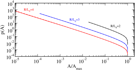
Figure 1: Probability density $P(A)$ vs $A_{s}/A_{max}$ for three different radii $R/L_{0}=2,3,4$. The dashed lines of the same color depict the histogram of the distribution generated by $10^{8}$ random picks for $A_{k}$.

Apparently, the probability to find a nucleus with coupling $A(r)$ increases quadratically with radius $r$: the distribution function $P(A)$ diverges for $A\to 0$ and requires a finite cutoff radius $R>L_{0}$ for which the envelope wave function has almost vanished and $\Psi(\vec{r})$ is approximately normalized in that sphere of radius $R$. Although the physics must be independent of this artificial cutoff $R$, only those nuclei with a significant coupling constant contribute to the dynamics of the central spin. Using the probability density for point of fixed radius $r$, $P(r)=3r^{2}/R^{3}$ and $P(A)dA=P(r)dr$, we derive the probability distribution

$$P(A,r_{0}) = \frac{3}{2}\frac{1}{r_{0}^{3}A}\sqrt{\log(A_{max}/A)}$$ (10)

where $A_{max}=A(0)=A_{s}v_{0}/(\sqrt{\pi}L_{0})^{3}$ and the ratio $r_{0}$ is defined as $r_{0}=R/L_{0}$. This distribution is shown in Fig. 1 for three different ratios $r_{0}=R/L_{0}=2,3,4$. We also added the histogram from $10^{8}$ randomly generated $A_{k}$ values as dashed line in the same color. They are nearly indistinguishable from the analytic function stated in (10). Note that this distribution function is almost identical to the one used by Coish and Loss.Coish and Loss (2004)

Using this probability distribution $P(A)$ it is straight forward to calculate the average $\bar{A}=\int dAP(A)A\approx A_{s}/N(R)$ where $N(R)=n_{0}4\pi R^{3}/3$ denotes the number of nuclei in the sphere of radius $R$. The square average $\bar{A}^{2}$ is approximately given by $\bar{A}^{2}\approx\sqrt{2}A_{s}^{2}[3\sqrt{\pi}N(R)N(L_{0})]^{-1}$. Both approximations become exact for $R\to\infty$.

Since the choice of the radius $R$ should be arbitrary, as long as $R>L_{0}$ and $|\Psi(R)|^{2}\approx 0$, the physical properties of the central spin model must not depend on $R$. This is clearly the case for $A_{s}=\sum_{k}A_{k}=N(R)\bar{A}$ since we have $N(R)$ different coupling constants. For the time scale $T^{*}$, the inverse rms of the Overhauser field, which governs the short time dynamics, we obtain

$$[T^{*}]^{-2} = \sum_{k=1}^{N}A_{k}^{2}=N(R)\bar{A}^{2}=A_{s}^{2}\frac{1}{3\sqrt{\pi}N(L_{0})}$$ (11)

which is also independent of the radius $R$. It is only dependent on $A_{s}$ and the number of nuclei which are located within the sphere defined by the length scale $L_{0}$ of the electronic envelope function. Using the parameters from above an estimate for $T^{*}\approx 30$ ns and a characteristic frequency $f=1/T^{*}\approx 32$ Mhz for electrons and a factor $10^{-1}-10^{-3}$ times smaller value for hole spins.

Although the cutoff $r_{0}$ controls the width of the distribution function $P(A,r_{0})$, the physics must remain invariant in the thermodynamic limit, when sending $N\to\infty$ first and then $r_{0}\to\infty$. In a finite size calculation, however, each random configuration of hyperfine couplings $\{A_{k}\}$ generated by $P(A,r_{0})$ yields a slightly different dynamics. To bridge between the typically $N(L_{0})\approx 10^{5}$ nuclear spins in real QDs and the numerical CET simulations of a spin bath with $N=20$, each configuration $\{A_{k}\}$ is normalized to a fixed $1/T^{*}=\sqrt{\sum_{k}A_{k}^{2}}$ which is the energy unit used in all calculations. Therefore, each configuration is characterized by exactly the same short time dynamics, and by averaging over typically $n=50-100$ different configurations we mimic a much larger spin-bath.

A word is in order about varying the cutoff $r_{0}$. For very large $r_{0}$, the ratio $a$ between the largest and the smallest hyperfine coupling is exponentially large and the probability of generating exponentially low coupling constants is large. In this case, we will end up with one or two large couplings $a_{k}=A_{K}T^{*}\to 1$, while all other are exponentially small for a fixed $N$. The resulting unphysical dynamics will be discussed in Sec. III.1 below.

In order to avoid this effect one could demand that the largest dimensionless coupling $a_{max}={\rm max}\{a_{k}\}$ must be a constant when varying $r_{0}$. This requires a simultaneous change of the bath size $N$ when varying $r_{0}$. Choosing $a_{max}=0.5$ ensures a reasonable distribution of dimensionless coupling constants $\{a_{k}\}$ since the sum of all other couplings squares must be $3/4$. For $r_{0}=1.5$ we can fulfill this condition with $N=18$ while for $r_{0}=1$ only $N=8$ would be sufficient. For $r_{0}=2$, however, we would need $N=42$ nuclear spins which is beyond the reach of the CET. For $r_{0}=2$ and $N=18$ we find $a_{max}=0.64$: this is only slightly larger than $0.5$ and implies that all other hyperfine constants still contribute $\approx 60\%$ to $T^{*}$. In our simulations, we typically us $r_{0}=1.5$ and $N=18$.

II.3 Definition of the spin-noise function

Experimentally the spin-noise is measured via fluctuations of the Faraday rotation angle using a linearly polarized probe laser in $z$-direction of the sample. The auto-correlation function of the Faraday rotation angle is equivalent to the symmetrized fluctuation function

$$S(t) = \frac{1}{2}\left[\left\langle S^{z}(t)S^{z}\right\rangle+\left\langle S^{z}S^{z}(t)\right\rangle\right]-\left\langle S^{z}\right\rangle^{2}$$ (12)

where $\left\langle S^{z}\right\rangle$ denotes the average spin-polarization which vanishes in the absence of an external magnetic field. The probe laser only weakly perturbs the system, and all expectation values are calculated using the equilibrium density operator. Since $S(t)$ is symmetric in time, the spin-noise spectrum

$$S(\omega) = \int_{-\infty}^{\infty}S(t)e^{-i\omega t}dt=\int_{-\infty}^{\infty}S(t)\cos(\omega t)dt\,.$$ (13)

From these definitions, we obtain the obvious sum-rule

$$\int_{-\infty}^{\infty}\frac{d\omega}{2\pi}\,S(\omega) = S(0)=\left\langle(S^{z})^{2}\right\rangle-\left\langle S^{z}\right\rangle^{2}$$ (14)

for the spin-noise spectrum. In the absence of an external magnetic field, its value is fixed to $1/4$ for a QD filled with a single electron or hole spin. This sum-rule is useful to test the accuracy of any numerical spin-noise calculation.

II.4 Connection between the spin-noise function and the real-time dynamics

The spin-noise measurements are performed in thermal equilibriumCrooker et al. (2010) at $T\approx 5\,\text{K}\rightarrow k_{B}T\approx 4\cdot 10^{-4}\,\text{eV}$. Since the intrinsic energy scale $A_{s}$ of the system is of the order $O(10^{-5}\,\text{eV})$ for electrons and even one order of magnitude smaller for holes, $\beta A_{s}\ll 1$ holds, and we can consider the coupled system consisting of the nuclear spin bath and the central spin in the limit of high temperature and being characterized by the initial density operator

$$\rho_{0} =\frac{1}{D}\underline{\underline{1}}\,,$$ (15)

where $D$ is the dimension of the Hilbert space and $\underline{\underline{1}}$ is the identity matrix. Using the commutator $\left[\rho_{0},S^{z}\right]=0$, we conclude: $\left\langle S^{z}(t)S^{z}\right\rangle=\left\langle S^{z}S^{z}(t)\right\rangle$.

If we prepare an initially fully polarized electron (hole) spin along the $z$-direction coupled to an incoherent nuclear spin bath, the density operator for such a system is given by

$$\rho_{p} =\rho_{0}(\underline{\underline{1}}+2S^{z})\,\,.$$ (16)

The time evolution $\left\langle S_{z}(t)\right\rangle$ for this initial condition

$$\left\langle S^{z}(t)\right\rangle_{\rho_{p}} = \textrm{Tr}\left[\rho_{p}S^{z}(t)\right]=\left(\left\langle S^{z}\right\rangle+2\left\langle S^{z}(t)S^{z}\right\rangle\right)$$ (17)

$$= 2\left\langle S^{z}(t)S^{z}\right\rangle=2S(t)$$

is equivalent to twice the correlation function $S(t)$ where the expectation values are calculated with respect to $\rho_{0}$. Therefore, $S(t)$ can also be interpreted as the dynamics of an initially fully polarized spin coupled to a bath at high temperature. In this limit, we still can neglect the spin polarization in Eq. (12) in a magnetic field, since the large field limit discussed below implies a large magnetic field in comparison to the hyperfine energy scale but still small compared to the temperature.

II.5 Quasi-static approximation for $\vec{B}=0$

MerkulovMerkulov et al. (2002) et al. proposed a quasi-static approximation (QSA) to calculate the short-time dynamics of an initially polarized electron spin which later has been extended to dot-confined hole spins by Testelin et al.Testelin et al. (2009) It is based on a separation of energy scales and, therefore, time scales. While a single nuclear spin just is exposed to the field generated by the single central spin whose magnitude is proportional to $A_{k}\ll A_{s}$, the electron spin precesses in a constant effective magnetic field $\vec{B}_{\text{eff}}$ provided by a frozen nuclear spin bath configuration $\left|\psi_{\rm bath}\right\rangle$

$$\vec{B}_{\text{eff}} = \frac{1}{\mu_{B}g_{e}}\sum_{k}A_{k}\left\langle\psi_{\rm bath}\right|\vec{I}_{k}\left|\psi_{\rm bath}\right\rangle=B_{\text{eff}}\vec{n}$$ (18)

for the time scale defined by the effective Larmor frequency $\omega_{\text{eff}}=g_{e}\mu_{B}|\vec{B}_{\text{eff}}|$ which is of the order of $O(A_{s})$. In this momentarily frozen field in the direction $\vec{n}=\vec{B}_{\text{eff}}/|\vec{B}_{\text{eff}}|$, the Bloch equations for the electronic spin dynamics have the simple solution

$$\left\langle\vec{S}(t)\right\rangle = \left(\vec{S}_{0}\cdot\vec{n}\right)\vec{n}+\left(\vec{S}_{0}-\left(\vec{S}_{0}\cdot\vec{n}\right)\vec{n}\right)\text{cos}(\omega_{\text{eff}}t)$$ (19)

$$+\left[\vec{n}\times\left(\vec{S}_{0}-\left(\vec{S}_{0}\cdot\vec{n}\right)\vec{n}\right)\right]\text{sin}(\omega_{\text{eff}}t),$$

with initial polarization of the electron spin $\vec{S}_{0}$.

The effective magnetic field is generated by a large number of small contributions from randomly oriented nuclear spins. Therefore, the direction is isotropically distributed over a unit-sphere, and, in the limit of large $N$, the magnitude of the effective field is described by the Gaussian probability distribution

$$W(\vec{B}_{\text{eff}}) =\frac{1}{\pi^{3/2}\Delta_{B}^{3}}\text{exp}\left(-\frac{\vec{B}_{\text{eff}}^{2}}{\Delta_{B}^{2}}\right),$$ (20)

$$\Delta_{B}^{2} =\frac{1}{2(\mu_{B}g_{e})^{2}}\sum_{k}A_{k}^{2}=\frac{1}{2(\mu_{B}g_{e}T^{*})^{2}}$$ (21)

whose width is defined by the fluctuation time scale $T^{*}$. Averaging the central spin dynamics (19) over the distribution function $W(\vec{B}_{\text{eff}})$

$$\left\langle\vec{S}(t)\right\rangle = \int d\Omega\int_{0}^{\infty}B^{2}\text{d}B\,W(\vec{B}_{\text{eff}})\vec{S}(t)$$ (22)

the QSA resultMerkulov et al. (2002) for $\vec{S}(t)=S^{z}(t)\vec{e}_{z}$

$$\left\langle S^{z}(t)\right\rangle = \frac{S^{z}_{0}}{3}\left[1+2\left(1-\left(\frac{t}{2T^{*}}\right)^{2}\right)e^{-\frac{1}{2}\left(\frac{t}{2T^{*}}\right)^{2}}\right]$$ (23)

$$= 2M(t)$$

has been obtained. It is straight forward to calculate its Fourier transformation $M(\omega)$

$$M(\omega) = \int_{-\infty}^{\infty}\text{d}t\,\text{e}^{-i\omega t}M(t)$$

$$= \frac{S_{0}}{3}\left[2\pi\delta(\omega)+\omega^{2}(\sqrt{8}T^{*})^{3}\sqrt{\pi}\text{e}^{-2(\omega T^{*})^{2}}\right]\,,$$

where $S_{0}=S^{z}_{0}/2$, because $S_{0}$ refers to the correlation function $S(t)$ instead of $\left\langle S^{z}(0)\right\rangle$. Since the QSA generates decoherence only by angular averaging, it lacks long-time decay and contains a large non-decaying contribution of $1/3$ of the initial spin-polarization $S_{0}$. This large non-decaying contribution defines the weight of the spin-noise $\delta$-function at $\omega=0$.

II.6 The Chebyshev expansion technique

II.6.1 Expansion of the time evolution operator

Since all our results have been obtained using the CET,Ezer and Kosloff (1984); Kosloff (1994); Weiße et al. (2006) we briefly review the CET, in order to introduce the notation used below.

The CETEzer and Kosloff (1984); Kosloff (1994); Weiße et al. (2006) has been developed 30 years ago and offers an accurate way to calculate the time evolution of a single initial state $|\psi_{0}\rangle$ under the influence of a general time-independent and finite-dimensional Hamiltonian ${\cal H}$:

$$|\psi(t)\rangle = e^{-i{\cal H}t}|\psi_{0}\rangle.$$ (25)

The main idea of the method is to construct a stable numerical approximation for the time-evolution operator $e^{-i{\cal H}t}$ that is independent of the initial state $|\psi_{0}\rangle$ and whose error can be reduced to machine precision for any given time $t$. Its limitation lies in the need to explicitly store certain states in the course of the calculation, which limits the size of the Hilbert space that can be handled.

There are different ways to expand the time-evolution operator. The most direct one is the conventional expansion of the exponent in powers of ${\cal H}$ using the definition of any operator function. One would like, however, to use an expansion that converges uniformly, independent of the initial state $|\psi_{0}\rangle$. The Chebyshev polynomials turned out to be such a suitable choiceEzer and Kosloff (1984). They are defined by the recursion relation

$$T_{n+1}(z)=2zT_{n}(z)-T_{n-1}(z),$$ (26)

subject to the initial conditions $T_{0}(z)=1$ and $T_{1}(z)=z$. Those polynomials can be used to expand any function $f(z)$ on the interval $-1\leq z\leq 1$. Explicitly, $f(z)$ is expressed as an infinite series

$$f(z) = \sum_{n=0}^{\infty}b_{n}T_{n}(z),$$ (27)

where the expansion coefficients $b_{n}$ are given by

$$b_{n} = \frac{2-\delta_{n,0}}{\pi}\int_{-1}^{1}dx\,\frac{f(x)T_{n}(x)}{\sqrt{1-x^{2}}}\,.$$ (28)

Using the integral representationAbramowitz and Stegun (1972) of the Bessel function

$$J_{n}(z) = \frac{i^{-n}}{\pi}\int_{0}^{\pi}d\vartheta e^{iz\cos\vartheta}\cos(n\vartheta)$$ (29)

and $T_{n}(\cos\vartheta)=\cos(n\vartheta)$, we immediately arrive for $z\in[-1:1]$ at

$$e^{-iz\tau} = \sum_{n=0}^{\infty}b_{n}T_{n}(z)$$ (30)

with the expansion coefficients $b_{n}=(2-\delta_{0,n})i^{n}J_{n}(\tau)$.

If the spectrum of the Hamiltonian is bound to $E_{\rm min}\leq E\leq E_{\rm max}$, the time-evolution operator $e^{-i{\cal H}t}$ can be expanded in the same fashion after mapping the Hamiltonian to the dimensionless $H^{\prime}=(H-\alpha)/\Delta E$ where we have defined the center of the energy spectrum $\alpha=(E_{\rm max}+E_{\rm min})/2$ and its half-width $\Delta E=(E_{\rm max}-E_{\rm min})/2$. Identifying $\tau=\Delta Et$ we arrive at

$$e^{-iHt}=\sum_{n=0}^{\infty}b_{n}(t)T_{n}(H^{\prime})\,$$ (31)

with

$$b_{n}(t) = (2-\delta_{0,n})i^{n}e^{-i\alpha t}J_{n}(\Delta Et).$$ (32)

Finally, applying Eq. (31) to the initial state $|\psi_{0}\rangle$ one obtains

$$|\psi(t)\rangle=\sum_{n=0}^{\infty}b_{n}(t)|\phi_{n}\rangle,$$ (33)

where the infinite set of states $|\phi_{n}\rangle=T_{n}({\cal H}^{\prime})|\psi_{0}\rangle$ obey the recursion relationWeiße et al. (2006)

$$|\phi_{n+1}\rangle=2{\cal H}^{\prime}|\phi_{n}\rangle-|\phi_{n-1}\rangle,$$ (34)

subject to the initial condition $|\phi_{0}\rangle=|\psi_{0}\rangle$ and $|\phi_{1}\rangle={\cal H}^{\prime}|\psi_{0}\rangle$.

Several comments are in order. First, all time dependence is confined in Eq. (33) to the expansion coefficients $b_{n}(t)$, which are independent of the initial state $|\psi_{0}\rangle$. Second, the Chebyshev recursion relation of Eq. (34) reveals the iterative nature of the calculations. Starting from the initial state $|\psi_{0}\rangle$, one constructs all subsequent states $|\phi_{n}\rangle$ using repeated applications of the “transformed” Hamiltonian ${\cal H}^{\prime}$. Third, since $J_{n}(x)\sim(ex/2n)^{n}$ for large order $n$, the Chebyshev expansion converges quickly as $n$ exceeds $\Delta Et$. This allows to terminate the series (33) after a finite number of elements $N_{C}$ guaranteeing an exact result up to a well defined order. Finally, the Chebyshev expansion has the virtue that numerical errors are practically independent of $t$, allowing access to very long times. The main limitation of the approach, as commented above, stems from the size of the Hilbert space, since each of the states $|\phi_{n}\rangle$ must be constructed explicitly.

For the application of the CET to the central spin model, an estimation of the upper and lower bound of the Hamiltonian is required entering the center of the energy spectrum $\alpha$ and its half-width $\Delta E$. Applying the power iteration method, the series

$$\left\lvert\varphi_{n}\right\rangle=\frac{{\cal H}^{n}\left\lvert\varphi_{0}\right\rangle}{\sqrt{\left\langle\varphi_{0}\right\rvert{\cal H}^{n}{\cal H}^{n}\left\lvert\varphi_{0}\right\rangle}}$$ (35)

converges to the eigenvector associated with the eigenvalue $\bar{E}$ the largest absolute value ${\rm max}\{|E_{\text{min}}|,|E_{\text{max}}|\}$. For $\lambda=1$, and $A_{k}>0$, one can show that the eigenvalue obtained by the power iteration determines $E_{\text{min}}$ while $E_{\text{max}}=\omega_{L}/2+A_{s}/4$. For the Ising regime, $\lambda\to\infty$, the largest eigenvalue $E_{+}$ and the smallest eigenvalue $E_{-}$ are exactly known

$$E_{\pm} = \pm\sqrt{\left(\frac{\omega_{L}}{2}\right)^{2}+\left(\frac{A_{s}}{4}\right)^{2}}$$ (36)

and for any finite $\lambda$, we interpolate between these to limits. Alternatively, one can set $\alpha=0$ and only use the eigenenergy $\bar{E}$ to define $\Delta E=2\bar{E}$. In either case, $\alpha$ and $\Delta E$ entering the Chebyshev expansion are easily obtained.

II.6.2 Evaluating traces

The original applicationDobrovitski and De Raedt (2003) of the CETEzer and Kosloff (1984); *Kosloff-94 focused on the dynamics of a single wave-function. We have extended the approach to thermodynamic ensembles to incorporate the incoherent spin-bath at high-temperature relevant to the experiments.

The expectation value of an arbitrary time-dependent observable $O$ is given by

$$\left\langle O(t)\right\rangle = \text{Tr}\left[\rho_{0}O(t)\right]=\sum_{i=1}^{D}\left\langle i\right\rvert\rho_{0}\text{e}^{iHt}O\text{e}^{-iHt}\left\lvert i\right\rangle$$ (37)

$$= \sum_{i=1}^{D}\left\langle i^{\prime}(t)\right|O\left|i(t)\right\rangle$$

where $\left\lvert i\right\rangle$ denotes a state of the complete basis set. $D=2^{N+1}$ grows exponentially with the number of bath spins, and the direct evaluation of the trace cannot be computed in moderate time for large $N$. In addition, the CET provides only the time evolution of a single state $\left|i(t)\right\rangle=\text{e}^{-iHt}\left|i\right\rangle$ and $\left|i^{\prime}(t)\right\rangle=\text{e}^{-iHt}\rho_{0}\left|i\right\rangle$.

Therefore, we employ a stochastical method discussed by Weisse et al..Weiße et al. (2006) It is based on the generation of $N_{s}$ random states $\left|r\right\rangle$ of the form

$$\left\lvert r\right\rangle = \sum_{i=1}^{D}\xi_{ri}\left\lvert i\right\rangle$$ (38)

with the real coefficients $\xi_{si}$ fulfilling the relations

$$\left\langle\left\langle\xi_{ri}\right\rangle\right\rangle = 0,$$ (39)

$$\left\langle\left\langle\xi_{ri}\xi_{r^{\prime}j}\right\rangle\right\rangle = \delta_{r,r^{\prime}}\delta_{i,j}$$ (40)

where $\left\langle\left\langle\cdots\right\rangle\right\rangle$ refers to the statistical average of these random numbers. Note that $\left|r\right\rangle$ is not a normalized state for $\xi_{si}$ fulfilling those relations. However, the trace of an operator $\hat{A}$ can be evaluatedWeiße et al. (2006) by

$$\left\langle\left\langle\frac{1}{N_{s}}\sum_{r=1}^{N_{s}}\left\langle r\right|\hat{A}\left|r\right\rangle\right\rangle\right\rangle = \frac{1}{N_{s}}\sum_{r=1}^{N_{s}}\sum_{i,j=1}^{D}\left\langle\left\langle\xi_{ri}\xi_{rj}\right\rangle\right\rangle\left\langle i\right|\hat{A}\left|j\right\rangle$$ (41)

$$= \sum_{i=1}^{D}\left\langle i\right|\hat{A}\left|i\right\rangle$$

by statistical average of the random numbers.

Using the self-averaging properties of $\xi_{ri}$ drawn from a Gaussian distribution, the trace is approximatedWeiße et al. (2006) by

$$\frac{1}{N_{s}}\sum_{r=1}^{N_{s}}\left\langle r\right|\hat{A}\left|r\right\rangle = \sum_{i=1}^{D}\left\langle i\right|\hat{A}\left|i\right\rangle+O\left(\frac{1}{\sqrt{N_{s}D}}\right)\,.$$ (42)

The error is well controlled and scales with $(N_{s}D)^{-1/2}$: only a few states $N_{s}$ are needed for an exponentially large Hilbert space. In our simulations we typically use $N_{s}=5$ different randomly generated states for the evaluation of the traces.

For very small Hilbert-spaces $N<10$, we have the reverse situation: the number $N_{s}$ of random states required for a small error might exceed the dimension of the Hilbert-space $D$. In such cases, the trace has been evaluated exactly.

II.7 Spin-noise spectra obtained from Chebyshev polynomial expansion

Since the time-dependent coefficients of the CET are known and are stated in Eq. (28), we can analytically perform the Fourier transformation of $S(\omega)$ in Eq. (13) and derive an explicit expression for the spin noise in terms of the momentum $\mu_{n,m}$ and a convolution of two Chebyshev polynomials

$$S(\omega) = \frac{2\pi}{\Delta E}\sum_{n,m=0}^{\infty}\mu_{n,m}\int_{-1}^{1-\frac{\omega}{\Delta E}}\text{d}\tilde{\omega}\,$$ (43)

$$\times\frac{T_{n}(\tilde{\omega})T_{m}(\tilde{\omega}+\frac{\omega}{\Delta E})}{\sqrt{(1-\tilde{\omega}^{2})(1-(\tilde{\omega}+\frac{\omega}{\Delta E})^{2})}}$$

for $\omega\geq 0$. While the convolution of two Chebyshev polynomials only depends on the half-width $\Delta E$ of the spectrum of $H$ and is independent of the dynamics, the momentum $\mu_{n,m}$ gather all Hamiltonian dependent information about the dynamics and are defined as

$$\mu_{n,m} = \frac{2-\delta_{n,0}}{\pi}\frac{2-\delta_{m,0}}{\pi}$$ (44)

$$\times\text{Tr}\left\{\rho_{0}T_{n}(H^{\prime})S^{z}T_{m}(H^{\prime})S^{z}\right\}\,.$$

and evaluated with the method presented in Sec. II.6.

The additional prefactors $g_{n}$

$$g_{n} = \frac{(N_{C}-n+2)\text{cos}\frac{\pi n}{N_{C}+2}+\text{sin}\frac{\pi n}{N_{C}+2}\text{cot}\frac{\pi}{N_{C}+2}}{N_{C}+2},$$ (45)

referring to as Jackson kernel,Weiße et al. (2006) considerably reduce the truncation errorWeiße et al. (2006) when evaluating the truncated series

$$S(\omega) = \frac{2\pi}{\Delta E}\sum_{n,m=0}^{N_{C}}g_{n}g_{m}\mu_{n,m}I_{n,m}(\frac{\omega}{\Delta E})$$ (46)

instead of the true infinite series given by Eq. (43). Since the function $I_{n,m}(x)$ defined as

$$I_{n,m}(x) = \int_{-1}^{1-x}\text{d}\tilde{\omega}\,\frac{T_{n}(\tilde{\omega})T_{m}(\tilde{\omega}+x)}{\sqrt{(1-\tilde{\omega}^{2})(1-(\tilde{\omega}+x)^{2})}}$$ (47)

is independent of the Hamiltonian, it can be calculated and stored independently, and later used in the summation (46) of the momenta.

From the orthogonality relation of the Chebyshev polynomials we can immediately conclude that only the momentum $\mu_{0,0}$ contributes to the spin noise sum-rule (14):

$$S(t=0) = \frac{1}{2\pi}\int_{-\infty}^{\infty}\text{d}\omega\,S(\omega)$$

$$= \sum_{n,m=0}^{N_{C}}\text{Tr}\left[\rho_{0}T_{n}(H^{\prime})S^{z}T_{m}(H^{\prime})S^{z}\right]\delta_{n,0}\delta_{m,0}$$

$$= \text{Tr}\left[\rho_{0}(S^{z})^{2}\right]=\frac{1}{4}.$$ (49)

Thus all spectral functions calculated from the CET exactly fulfill the sum-rule independent of the number $N_{C}$ of included Chebyshev polynomials.

III Dephasing of an electron spin: the isotropic central spin model

We begin with the discussion of the spin dynamics for a single electron confined in a single quantum dot by investigating the isotropic CSM with $\lambda=1$. For all simulations of the real-time dynamics, we used the CET for the evolution of the states in a system of $N$ bath spins for a fixed configuration $\{A_{k}\}$ drawn from the probability distribution $P(A,r_{0})$ stated in Eq. (10). Since the number of bath sites is limited to $N\approx 20$, we average over typically $50$ configurations $\{A_{k}\}$. By this averaging we minimize finite size oscillations and essentially mimic an effectively larger bath.

III.1 Benchmarks

In order to establish the virtue and the limitations of the CET approach in combination with a statistical evaluation of the traces, we have investigated the influence of (i) the number of bath spins $N$, (ii) the order of the largest polynomial $N_{C}$, (iii) the number of random states $N_{s}$.

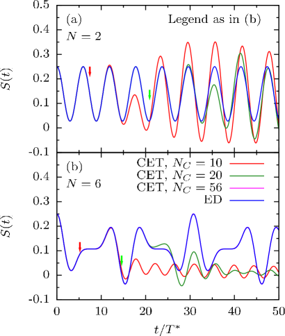
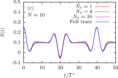
Figure 2: (color online) Benchmark for the CET calculating the time evolution of the spin correlation function $S(t)$ for uniform coupling constants $A_{k}=\frac{A_{s}}{N}$. Two different orders $N_{C}$ of the expansion are compared to ED for $N=2$ (a) and $N=6$ (b) bath spins. After the time scale indicated by the arrows the CET-error exceeds $O(10^{-3})$. In (a)-(b) the occurring traces have been calculated exactly and no error from the statistical evaluation of traces enters. (c) treats this error for $N=10$, by comparing results for a varying number $N_{s}$ of random states to a result taking the full trace into account with $N_{C}=66$.

To benchmark the CET in small test systems accessible to exact diagonalisation (ED), we restrict ourselves to uniform coupling constants $A_{k}=A_{s}/N$ at first, defining $T_{1}^{*}=T^{*}=\sqrt{N}/A_{s}$. We compare results obtained by ED with CET calculations for $N=2,6$ and three different CET orders $N_{C}$ in Figs. 2 (a)-(b). For such small systems, we evaluate the traces for the momenta $\mu_{n,m}$ in (44) exactly, since the number $N_{s}$ of randomly generated states needed for an accurate statistical evaluation of the traces exceeds the dimension of the Hilbert space. Therefore, the only error of the CET data at longer times in Figs. 2 (a)-(b) arises from the finite $N_{C}$ while for the short-time dynamics up to $t<t_{\rm max}(N_{C})$ an essentially exact result is obtained.

The convergence of the CET for any given time $t$ is ensured by the analytic properties of the Bessel functions of large order given by $J_{n}(\Delta Et)\sim\left(e\Delta Et/2n\right)^{n}$. The vertical arrows in Figs. 2 (a)-(b) indicate where this estimate exceeds the value $10^{-3}$ for $N_{C}=10$ and $20$. Apparently the CET reproduces the exact ED results accurately up to this time. Thus, the order of the CET for all further calculations is determined by the smallest $N_{C}$ fulfilling the condition $\left(e\Delta Et_{\rm max}/2N_{C}\right)^{N_{C}}\leq 10^{-3}$, where $t_{\rm max}$ is the largest time of interest. For $N=6$ and $t_{\text{max}}(N_{C})/T^{*}=50$ this estimate yields $N_{C}=56$. Consequently, the CET renders the ED result exactly up to $t/T^{*}=50$. To illustrate the deviations at larger time for an insufficiently large $N_{C}$, $S(t)$ is plotted for the additional two values $N_{C}=10,20<56$ in Fig. 2 (b).

Fig. 2(c) illustrates the effect of the error arising from the statistical evaluation of traces for $N=10$ bath spins. The CET-result where the traces have been exactly calculated (blue line) is serving as reference. Since the error of the statistical evaluation is of the order $O((N_{s}D)^{-1/2})$, each ascending value for $N_{s}$ shown in Fig. 2 (c) reduces the remaining error by a factor $2$ independent of the time $t$. This decrease of the statistical error is clearly visible. For $N=10$, where the Hilbert space has the dimension of $D=2^{11}=2048$, our results with $N_{s}=16$ random states already converged enough to be optically almost undistinguishable from the exact calculations. By choosing either a large number of random states $N_{s}$ or a large number of nuclei $N$, we are able to obtain an accurate representation of the exact evaluation of the traces.

The physics of the CSM with uniform coupling constants $A_{k}=A/N$ is well understood.Khaetskii et al. (2003) For a system with only two bath spins we observe a coherent oscillation as depicted in Fig. 2(a) since the central spin effectively only interacts with the triplet state formed by the two bath spins while the singlet is decoupled. The oscillation frequency is given by the full width $2\Delta E=E_{\text{max}}-E_{\text{min}}$ of the Hamiltonian’s spectrum. For larger systems the dynamics is still coherent and of the form as exemplarily shown for $N=6$ and $N=10$ in Figs. 2 (b)-(c). The short time dynamics for $N>3$ is governed by $T^{*}$ and the recurrence time $T_{\rm rec}$, where $S(T_{\rm rec}+t)=S(t)$, increases linearly with the bath size since the differences of the eigenenergies are commensurable. We find $T_{\rm rec}\approx 30T^{*}$ for $N=6$ and $T_{\rm rec}\approx 40T^{*}$ for $N=10$.

III.2 Results in the absence of an external magnetic field

III.2.1 Influence of the distribution function on the real-time dynamics

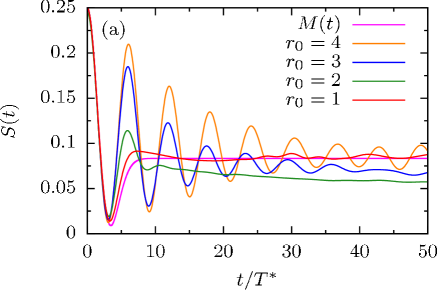
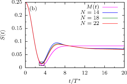
Figure 3: (color online) The spin correlation function $S(t)$ for randomly generated coupling constants $A_{k}$ calculated via CET. Each shown curve has been averaged over $n=50$ different random realizations of couplings. (a) Short-time evolution of $S(t)$ for increasing $r_{0}$ with $N=18$. (b) The analytical result $M(t)$ in comparison to calculated data for increasing bath size $N$ based on a fixed ratio $r_{0}=R/L_{0}=1.5$. The inset shows the area marked by the box.

Now we discuss the influence of randomly generated coupling constants $A_{k}$ onto the time evolution of the spin-correlation function $S(t)$. In numerically accurate simulations of the real-time dynamics using a statistical evaluation of the Bethe-ansatz equations,Faribault and Schuricht (2013a, b) the maximum number of bath spins $N\approx 45$ still remains several orders of magnitude smaller than the $10^{5}$ nuclear spins present in experimental samples. The dynamics of small systems is influenced by the range of coupling constants defining the ratio $a=A_{\text{max}}/A_{\text{min}}$ between the largest and the smallest coupling constant. Increasing $a$ at constant $N$ increases the number of nuclear spins which are only very weakly coupled to the electronic spin. In addition the deviation of the average square, $\left\langle A\right\rangle^{2}$ and the fluctuation $\left\langle A^{2}\right\rangle$ increase. The short and intermediate dynamics is dominated by a decreasing number of bath spins for a fixed $N$, while thevery weakly coupled spins are only contributing significantly at extremely long times.

In a statistical evaluation of the exact Bethe ansatz equationsFaribault and Schuricht (2013a, b) the fixed set of $A_{k}=A/N\exp[-(k-1)/(N-1)]$ has been chosen, leading to the ratio $a={\rm e}$. A recent TD-DMRGStanek et al. (2013) study has pushed the limit to up to $N=100-1000$ nuclear bath spins. In this study, the configurations of $\{A_{k}\}$ have been drawn from $P(A)=const$ on the interval $A_{0}[1/2,1]$, corresponding to a ratio $a=2$. For the first distribution, the fluctuation $u=\left\langle A\right\rangle^{2}/\left\langle A^{2}\right\rangle\approx(1+1/e)/(1-1/e)/2\approx 1.082$, while the distribution $P(A)=const.$ yields $u=28/27$. In both cases $u\approx 1$ holds which does not differ significantly from $A_{k}=const$. Therefore, the non-decaying fraction of the spin polarization remains close to the QSA result.

In the distribution function $P(A,r_{0})$, defined in Eq. (10), the cutoff ratio $r_{0}$ directly translates into the ratio $a=\exp(r_{0}^{2})$. For large $r_{0}$ the probability $P(A,r_{0})$ is high for adding more and more nuclei to the system whose interaction with the central spin is negligible, e. g. for $r_{0}=4$ the ratio between the largest and smallest coupling constant $A_{k}$ has already reached $A_{\text{max}}/A_{\text{min}}\approx 10^{7}$. In order to obtain results faithfully representing a larger system, a set of several $A_{k}$ must be taken into account for each order of magnitude which is impossible for a system size of only $N=20$ bath spins.

Fig. 3 (a) illustrates the influence of the cutoff $r_{0}$ onto the real-time dynamics. The results are calculated for $N=18$ bath spins and averaged over $n=50$ different random configurations $\{A_{k}\}$ to reduce the influence of fluctuations and effectively take more nuclei into account. We added the QSA result $M(t)$ stated in Eq. (23) as a guide for the short-time dynamics obtained from a random nuclear field approximation in the thermodynamic limit $N\to\infty$. All CET curves perfectly coincide with $M(t)$ for very short time scales $t/T^{*}<3$.

For $r_{0}=1$, the ratio $a=e$, and only significant coupling constants of the same order of magnitude are taken into account. The polarization saturates approximately at the value $S(0)/3$ as predicted by the QSA. However, slight deviations between the CET curve and $M(t)$ are observed for times $t/T^{*}>3$. Nevertheless the CET short-time dynamics and results obtained by other approachesFaribault and Schuricht (2013a, b); Stanek et al. (2013) agree remarkably well with each other and with the QSA. This indicates that the generic dynamics can already be obtained by a rather small numbers of bath spins.

For increasing cutoffs $r_{0}>1$, the short-time dynamics of $S(t)$ evolves from passing through a single minimum as described by the QSA curve to a damped oscillation as depicted in Fig. 3(a). This behavior is easily understood by the distribution of coupling constants in any of the random configurations $\{A_{k}\}$. For a large cutoff $r_{0}$ and a fixed number of bath spins $N$, the number of nuclei which couple to the central spin with a coupling constant $A_{k}/A_{s}=O(1)$ becomes very small in $\{A_{k}\}$ due to the increasing probability to find a small coupling. Essentially we see a similar coherent motion as in Fig. 2(a) involving only one or two bath spins with the strongest coupling constants, while the slow dephasing is induced by the remaining very weakly coupled nuclear spins. Therefore, we conclude that such choices of the cutoff $r_{0}$ do not render the dynamics for $N\to\infty$ when working with a fixed and small $N$.

Fig. 3(b) focuses on the bath-size dependency of the short-time evolution of $S(t)$ for $N=14,18,22$ and fixed $r_{0}=1.5$. This cutoff would correspond to $N(R)\approx 10^{5}$ in a real system, implying a ratio $a\approx 8$. The figure compares exact simulations for three different bath sizes to the QSA result $M(t)$ and demonstrate the fast convergent with the bath size for $r_{0}=1.5$.

The initial decay of $S(t)$ is well described by $M(t)$ and for increasing $N$ the exact finite size curves approach the QSA solution for short-time scales. But after the initial decay the central spin’s polarisation drops below the value predicted by the QSA approach. This deviation arises from the contribution of the small coupling constants, whose interaction with the central spin is too weak to have major influence on the short time behavior of $S(t)$, but on large time scales the small couplings become dominant. Since the QSA result is based on the assumption of a static bath, it is not surprising that it is only able to describe the short-time and intermediate-time evolution of the central spin that is dominated by the strongly coupling nuclei.

III.2.2 The influence of $r_{0}$ onto the long-time limit

The deviation of the non-decaying fraction of the spin-polarization from the QSA value of $S(0)/3$ observed in Fig. 3(b) justifies a more detailed analysis.

The influence of $r_{0}$ onto the long-time limit is depicted in Fig. 4(a). With increasing $r_{0}$ we observe two effects: (i) the non-decaying part of the polarization $S_{\infty}=\lim_{t\to\infty}S(t)$ is decreasing, (ii) the relaxation time from the pre-equilibrated intermediate state reached after a short transient time of the order of $O(10T^{*})$ into the steady-state is increasing. Since the weakly-coupled nuclei can only contribute on large-time scales, the second observation is intuitively clear due to the increasing number of weakly coupling nuclei with increasing $r_{0}$ and fixed $N$.

The first observation can be also understood within a simple argument. In the QSA approach, no spin polarization transfer between the central spin and the spin bath can occur since the nuclear magnetic field has been treated statically. The spin decay is purely driven through dephasing by averaging over the random and isotropic effective magnetic field distribution yielding a finite steady-state value $S_{\infty}=S(0)/3$.

Recent Bethe-ansatz calculationsFaribault and Schuricht (2013a, b) up to $N=44$ nuclei confirm that the non-decaying fraction of the spin-polarization depends on the distribution of the coupling constants. In any finite size representation of the model with a small number of coupling constants $\{A_{k}\}$ a finite non-decaying fraction of the spin-polarization is found. This fraction, however, decreases when additionally weak coupling nuclear spins have been added. Faribault et al. gave an analytical argumentFaribault and Schuricht (2013b) why there must be a finite non-decaying fraction of the spin-polarization in any finite-size system, where the distribution of coupling constants $\{A_{k}\}$ is limited to the same order of magnitude. This agrees perfectly with our findings for a finite size system.

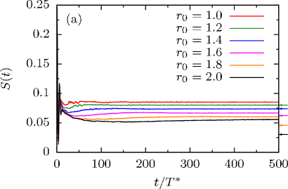
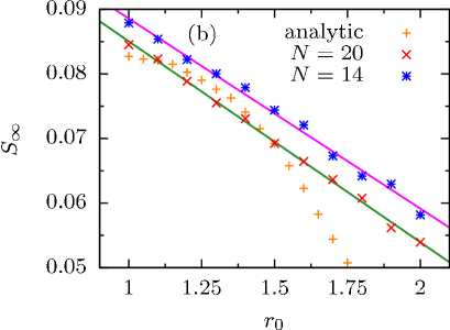
Figure 4: (color online) The behavior of $S(t)$ on long-time scales for different values of $r_{0}$ and $N=18$ (a). Each shown curve has been averaged over $n=50$ different random configurations $\{A_{k}\}$ of couplings. The colored arrows indicate the long-time values for $S_{\infty}$ predictedMerkulov et al. (2002) from the fluctuation ratio $u=\left\langle A^{2}\right\rangle/\left\langle A\right\rangle^{2}$. (b) The non-decaying fraction $S_{\infty}$, obtained by averaging the data over the calculated data points in the interval $\frac{t}{T^{*}}\in[450:500]$, vs. the cutoff $r_{0}$ for two different system sizes $N=14,20$. The straight lines are linear fits. The analytical predictions using the fluctuation ratio $u$ are added for comparison.

In contrast to exact evaluations of small systems, approximate treatmentsMerkulov et al. (2002); Khaetskii et al. (2002); Zhang et al. (2006b); Coish and Loss (2004) of the model allows to access the thermodynamic limit. Such treatments require the neglecting of higher order correlation effects and predict a finite non-decaying fraction. Taking into account non-Markovian contributions in second order of the transverse coupling,Coish and Loss (2004) leads to a non-exponential correction to the mean-field solution stated in Eq. (23) of the form $1/\log t$ in the absence of a magnetic field in the decay to a finite steady-state limit. Even though we observe a non-trivial transient behavior with a very slow decay between $100<t/T^{*}<1000$ the data is not sufficient to extrapolate a $[\log t]^{-\alpha}$ correction or a power-law decay to the non-decaying fraction from the data presented in Fig. 4(a). However, we have been able to extract a power-law behavior from the low-frequency properties of spin-noise spectra which will be discussed in Sec. III.3.

For bridging to the experiments we can ask the question what is the asymptotic non-decaying fraction of spin-polarization in the thermodynamic limit $r_{0}\to\infty$ and $N\to\infty$. In order to shed some light on this question within the framework of the CET approach, we have investigated the scaling properties of the non-decaying fraction of the polarization with respect to $r_{0}$ for two bath sizes $N=14,20$ in the interval $1\leq r_{0}\leq 2$, in which $S(t)$ has reached a steady-state limit as shown in Fig. 4(a). The short time dynamics is always governed by the time-scale $T^{*}$ and agrees very well with the QSA result.

The long-time limit is plotted as function of the cutoff $r_{0}$ for two different bath sizes $N$ in Fig. 4(b). The steady-state polarisation decreases linearly with $r_{0}$ for $r_{0}\leq 2$. Since the CET dynamics does not properly represent the large $N$ limit for $r_{0}$ exceeding $r_{0}>2$, as illustrated in panel (a) and discussed above, no data is shown for such cutoffs.

The linear scaling of $S_{\infty}$ as function of $r_{0}$ suggests that the non-decaying part of the central-spin polarization should vanish when the influence of very large numbers of small coupling constants is taken into account. Extrapolating our linear fit to the data for $N=20$ indicates that this is the case for $r_{0}\approx 3.7$, corresponding to a ratio $a\approx 10^{6}$. However, with increasing of the number of bath spins $N$, the predicted cutoff $r_{0}$ for that $S_{\infty}$ should vanish decreases as exemplified by the fit to two different spin bath dimensions in Fig. 4(b).

Our scaling analysis indicates that the spin correlations will completely decay at infinitely long times in the thermodynamic limit, e.g. $N\to\infty$ and then $r_{0}\to\infty$. This finding is fully consistent with an extension of the QSA which takes into account the long-time fluctuations of the nuclear magnetic field. Averaging Eq. (19) over times larger than the electron spin-precession time but much smaller than the nuclear spin precession time, the spin precession contribution vanishes and only the term $(\vec{S}_{0}\vec{n})\vec{n}$ survices. After inclusion of the explicit time-dependence of the nuclear field $\vec{B}_{\rm eff}=B_{\rm eff}\vec{n}(t)$ and spin, the ensemble average is given by Eq. (12) in Ref. [Merkulov et al., 2002]

$$\left\langle\vec{S}(t)\right\rangle = \left\langle\vec{n}(t)[\vec{n}(t)\vec{S}(t)]\right\rangle$$ (50)

Since $[\vec{B}_{\rm eff}(t)\vec{S}(t)]$ accounts for the total energy of the central-spin model, it is a conserved quantity and time independent: $[\vec{B}_{\rm eff}(t)\vec{S}(t)]=[\vec{B}_{\rm eff}(0)\vec{S}(0)]$. Furthermore the nuclear-spin-spin correlation function is isostropic leading to

$$\left\langle\vec{S}(t)\right\rangle = \gamma(t)\frac{\vec{S}(0)}{3}$$ (51)

where $\gamma(t)=\left\langle\vec{n}(t)\vec{n}(0)\right\rangle$ is defined as correlation function of the nuclear spin orientation.

For the long-time limit, $\gamma(t)$ approaches a stationary valueMerkulov et al. (2002) and is only dependent on the ratio $u=\left\langle A^{2}\right\rangle/\left\langle A\right\rangle^{2}$. We added our estimates for $S_{\infty}$ using $\gamma(u)$ derived in Ref. Merkulov et al., 2002 as horizontal arrows in Fig. 4(a) as well as crosses labeled “analytic“ into Fig. 4(b). Although our finite size scaling qualitatively agrees with a decreasing $\gamma(u)$ for increasing $r_{0}$, the functional form of $\gamma(u)$ differs from our linear scaling. This might be related to the change of the largest hyperfine coupling when varying $r_{0}$ for fixed $N$. Keeping both $T^{*}$ and the largest hyperfine coupling fixed requires the increase of $N$ when increasing $r_{0}$. This would accelerate the decrease of $S_{\infty}$ when increasing $r_{0}$ in closer agreement with $\gamma(u)$.

Another argument of why the non-decaying fraction $S_{\infty}$ must vanish in the long-time limit for $N\to\infty$ in QDs with smooth electronic confinement potential was given by Chen et al.Chen et al. (2007) based on the distribution function of the $A_{k}$. Although the total angular momentum in the isotropic CSM is conserved it will be equally redistributed onto all nuclear spins at large times. Since angular momentum transfer from the central spin to the nuclear spin $k$ occurs on a time scale $t>1/A_{k}$, only those spins within a given radius $R(t)=L_{0}[\ln(A_{0}t)]^{1/2}$ can contribute to the spin decay using the Gaussian envelope function (9) and $A_{0}=A(R_{k}=0)$. Only the strongly coupling spins in the sphere with radius $R_{s}=R(T^{*})$ contribute to the short-time dynamics up to the time $t$. Therefore, the central spin should decay as

$$\left\langle S^{z}(t)\right\rangle \propto \frac{N(R_{s})}{N(R(t))}\propto[\ln(A_{0}t)]^{-3/2}$$ (52)

in the long time limit $t\gg T^{*}$ in three dimensions and its expectation value vanishes for $t\to\infty$. Hence, the non-decaying fraction of the central spin-polarization must vanish in the thermodynamic limit. In any finite size calculation,Bortz and Stolze (2007); Bortz et al. (2010); Stanek et al. (2013); Faribault and Schuricht (2013a, b) however, there exist a smallest coupling constant $A_{\rm min}$ which limits the time scale beyond which the exact finite-size calculation will deviate from the thermodynamic limit.

III.2.3 Summary

Before we move on to the discussion of the spin noise spectra, we briefly summarize the results of this section. We have demonstrated the accuracy of the CET by a comparison of the real-time dynamics with small systems exactly solvable using ED. While in principle arbitraryly long times could be reached with the CET approach, it is limited by the largest polynomial order $N_{C}$ which has been included in the calculation. We have established the quality of the statistical evaluation of the momentum $\mu_{n,m}$ entering the extension of the CET approach to ensemble averages. The short-time dynamics is governed by the time scale $T^{*}$ and agrees qualitatively well with the QSA result. However, we observe small deviations which can be traced to (i) the distribution of the coupling constants $A_{k}$, to (ii) the number of bath spins and to (iii) the ratio between the largest and the smallest $A_{k}$. The larger this ratio is for fixed number of bath spins $N$, the smaller the number of bath spins which couple with an $A_{k}=O(1/T^{*})$, the less bath spins contribute effectively to the short time dynamics. The finite value of $S_{\infty}$ in a finite-size system depends on the distribution function $P(A)$.

III.3 Spin noise spectra

In recent experiments,Crooker et al. (2010); Dahbashi et al. (2012); Li et al. (2012); *ZapasskiiGreilichBayer2013 the spin noise spectra have been measured in QD ensembles. Assuming independent QDs, it is sufficient to average the generic spin-noise spectrum $S(\omega)$ over the distribution of time scales $T^{*}$ and $g$-factors to make a connection to the experimental data. Therefore, we focus on calculating the spin-noise spectrum $S(\omega)$ for a single QD first and postpone the discussion to spin-noise spectra for QD ensembles to Sec. V.

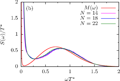
Figure 5: (color online) The spin-noise spectrum $S(\omega)$ in the absence of an external field for $r_{0}=1.5$. Panel (a) illustrates the convergence properties of the CET for varying $N_{C}$ and the effect of averaging results for several ($n$) configurations of the coupling constants $A_{k}$ based on $N=18$ bath spins and $r_{0}=1.5$. Panel (b) focuses on the finite bath size effects where we have averaged over $n=50$ different configurations $\{A_{k}\}$. $M(\omega)$ denotes the Fourier transformation of the semi-classical result where the $\delta$-peak in $M(\omega)$ at $\omega=0$ has been approximated by a Lorentzian.

A realistic modelling of the QD requires the treatment of the order $O(10^{5})$ nuclei. Even on a fine frequency scale, the noise spectrum will be continuous while $S(\omega)$ obtained from an exact simulation for $\sim 20$ bath spins with a single distribution $\{A_{k}\}$ clearly reflects the spectrum’s discrete character. In order to recover a continuous spectrum from the finite size CET calculation, we use two different ingredients: (i) averaging over random distributions $\{A_{k}\}$ and (ii) choosing a rather low order $N_{C}$ in the CET calculations. The averaging over several random distributions $\{A_{k}\}$ mimics a larger number of nuclei than contained in a single configuration. By artificially reducing $N_{C}$, we can effectively add a broadening to the individual $\delta$-peaks of the finite size spectrum which would only be precisely recovered in the limit $N_{C}\to\infty$. Increasing $N_{C}$ systematically increases the frequency resolution which we have employed to reveal a power-law in the low-frequency spin-noise spectrum. Note that no spectral weight is lost by this procedure since the sum-rule (14) is exactly fulfilled for arbitrary $N_{C}$.

In order to illustrate the effect of those two ingredients, we show a direct comparison of $S(\omega)$ for a single configuration ($n=1$) and data averaged over $n=100$ random configurations $\{A_{k}\}$ with $N_{C}=400$, $r_{0}=1.5$ and $N=18$ in Fig. 5(a). Additionally, the corresponding spectrum for a lower order $N_{C}=100$ of the CET and a reduced number of configurations $n=50$ has been added. While $S(\omega)$ obtained from a single configuration displays a clear signature of a superposition of discrete peaks a quasi-continuous spectrum is generated by the configuration averaging.

The calculations with a lower Chebychev order $N_{C}=100$ reproduce the calculations for $N_{C}=400$ excellently, except at small frequencies being consistent with linear scaling of the largest accessible time scale with $N_{C}$. Even though it would be sufficient to use rather small $N_{C}$ for an accurate description of the short-time dynamics, the numerical effort increases substantially to access the low frequency behavior of the spin-noise spectrum.

Based on the largest accessible time discussed in Sec. III.1, the smallest accessible frequency of the CET is given by $\omega_{\text{min}}\geq 10^{3/N_{C}}\pi\text{e}\Delta E/N_{C}$. Note that there are two limiting factors to the accessibility of small frequencies in our simulations: the finite $N_{C}$ and the finite cutoff $r_{0}$ which set the boundary to the lowest $A_{k}$ and therefore, the lowest non-zero excitation energy of the system. Choosing a larger $N_{C}$ than required by the means of this lowest excitation energy does not add additional information to the finite frequency spectrum but only sharpens the $\delta(\omega)$-peak.

The spectral functions $S(\omega)$ depicted in Fig. 5(b) for increasing number of bath spins and $r_{0}=1.5$ correspond to the time resolved data shown in Fig. 3(b). We note the fast convergence of $S(\omega)$ as function of $N$. We also added the QSA spin noise $M(\omega)$ stated in Eq. (II.5). The $\delta$-peak in $M(\omega)$ at $\omega=0$ has been approximated by a Lorentzian, and its spectral weight is given by the non-decaying fraction of the spin polarization.

The high-frequency part of $S(\omega)$ agrees remarkably well with the QSA spin-noise spectrum $M(\omega)$ rendering the excellent agreement in the short-time dynamics between both approaches. As expected, the broad high-frequency peak is centered at $1/T^{*}$ and its width given by $1/2T^{*}$. However, we notice significant deviations between $M(\omega)$ and $S(\omega)$ for smaller frequencies. Those differences also reflect the different transient behavior at times $t\gg T^{*}$ depending on the configurations of $\{A_{k}\}$.

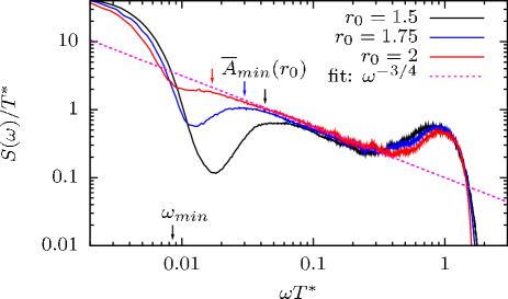
Figure 6: (color online) $S(\omega)$ vs $\omega T^{*}$ on a log-log scale for different values of $r_{0}=1.5,1.75,2$. The dashed line is a fit to the low-frequency behavior above the resolution-broadened $\delta(\omega)$-peak. The smallest accessible frequency $\omega_{\rm min}$ and the expectation value of the smallest contributing coupling constant $\overline{A}_{\text{min}}$ are indicated by arrows. Parameters: $N_{C}=1000,n=100,N=18,b=0$.

At low frequencies a small shoulder around $\omega T^{*}\approx 0.1$ is observed in $S(\omega)$ (green curve) in Fig. 5(a) when using $N_{C}=400$ and $n=100$ configuration averages. This indicates the existence of an additional low-frequency feature in $S(\omega)$, that is not covered by the QSA result, located above the resolution-broadened zero-frequency $\delta$-peak and below the Gaussian type high-energy peak around $\omega T^{*}\approx 1$.

In order to reveal the shape and nature of the low frequency part of the spin-noise spectrum in greater details, we have pushed the CET order to $N_{C}=1000$ to significantly increase the frequency resolution to $\omega_{\rm min}T^{*}=8.5\cdot 10^{-3}$. As depicted in Fig. 6, now the resolution-broadened $\delta(\omega)$-peak, whose full-width half maximum can be estimated by $2\omega_{\rm min}$, is well separated from the remaining low-frequency part of $S(\omega)$: the shoulder has evolved into a threshold-type behavior with a crossover around $\omega T^{*}\approx 0.03$ defined by the smallest excitation energy of the finite size system. A power law $\propto\omega^{-3/4}$ can be fitted in this region over approximately one decade and is indicated as dashed line. At larger frequencies, the previously discussed Gaussian-like peak remains visible and is centered around $\omega T^{*}\approx 1$.

The $r_{0}$-dependency of the crossover scale separating the low-energy feature in $S(\omega)$ from the resolution-broadened $\delta(\omega)$-peak is clearly visible in Fig. 6. Increasing $r_{0}$ extends the frequency range which can be fitted by $\propto\omega^{-3/4}$ to lower frequencies. The cutoff parameter $r_{0}$ determines the smallest hyperfine coupling $A_{k}$ contained in the configurations $\{A_{k}\}$ and, therefore, the smallest excitation energy in the system. We have indicated the value $\bar{A}_{\rm min}(r_{0})=\left\langle{\rm min}[A_{k}]\right\rangle$ averaged over all configurations $\{A_{k}\}$ by an additional vertical arrow in Fig. 6. Apparently, $\bar{A}_{\rm min}(r_{0})$ determines the low-frequency crossover scale to the power-law behavior.

We have demonstrated in Fig. 4 that the non-decaying fraction of the central spin polarization and, hence the spectral weight of the $\delta(\omega)$ peak decreases with increasing $N$ and $r_{0}$ and eventually vanishes in the thermodynamic limit.Chen et al. (2007) Hence, spectral weight of the $\delta(\omega)$-peak is transferred to the low-frequency part of $S(\omega)$ dominating the long-time properties of the spin correlation function $S(t)$. We conjecture that the observed finite low-energy crossover scale is approaching zero-frequency in the limit $r_{0}\to\infty$ and $N\to\infty$.

Restricted by the finite size of the spin bath and the frequency resolution, our numerical data is not accurate enough to predict the precise analytic form of $S(\omega)$ in the thermodynamic limit. The guide-to-the-eye fit to our data, however, would suggest $S(\omega)\propto\omega^{-3/4}$ implying a $1/t^{1/4}$ decay at long-time scales. This finding is consistent with the prediction $S(t)\propto\ln^{-3/2}(t)$, because in the intermediate time regime we can access via the CET both findings are almost indistinguishable in the time domain. To predict a deviation a fit over more than one decade is necessary.

III.4 Magnetic field dependence of the spin noise

III.4.1 Transversal magnetic field

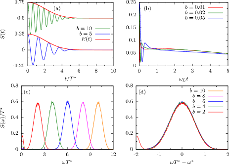
Figure 7: (color online) All shown simulations have been averaged over $n=50$ configurations. The spectral functions are all based on $N_{C}=100$. (a) The correlation function $S(t)$ for two different values of $b$. To distinguish the results for different $b$ an offset of $0.5$ has been added to the upper curve. The function $E(t)=\frac{1}{4}\text{exp}\left(-\frac{1}{2}\left(\frac{t}{2T^{*}}\right)^{2}\right)$ approximates the envelope of the signals. (b) $S(t)$ for small external field strengths. (c) The renormalized spin-noise function $S(\omega)$ for $b=2,4,...,10$. (d) The same data as shown in (c) shifted by $\omega^{*}=\sqrt{b^{2}+\frac{1}{2}}$, pointing out that the width of the occuring maxima is given by $T^{*}$ and that $\omega^{*}$ is the exact frequency of the occuring spin precession. Parameters: $N=20,r_{0}=1.5$.

Adding a transversal magnetic field $B_{x}$ to the system has two important effects on the time evolution of the correlation function $S(t)$. First, it breaks the conservation of the total polarization along the $z$-axis. Second, the short-time dynamics is now governed by a shifted time scale $1/T^{{}^{\prime}*}(b)=\sqrt{(T^{*})^{-2}+2\omega^{2}_{L}}$ which evolves continuously from $(T^{*})^{-1}$ with the external magnetic field. This can be either analytically derived from the von-Neumann equation or can be extracted from the numerical data for large $b$ as depicted Fig. 7(d).

Applying a large external magnetic field $b=\omega_{L}T^{*}\gg 1$ causes a damped oscillation in $S(t)$ whose dimensionless frequency is given by $\omega^{*}=\sqrt{b^{2}+1/2}$. Since the hyperfine interaction remains the origin of dephasing, the characteristic time scale of the decay is governed by the intrinsic time scale $T^{*}$. Fig. 7(a) demonstrates this behavior for two different magnetic field strengths fulfilling $\omega_{L}T^{*}>1$. Additionally the function

$$E(t) = \frac{1}{4}\exp\left[-\frac{1}{2}\left(\frac{t}{2T^{*}}\right)^{2}\right]$$ (53)

has been added as an approximation to the envelope of the real-time dynamics.

Fig. 7(c) shows the spin-noise spectrum $S(\omega)$ for five different magnetic field strengths $b=2,4,6,8,10$. The resulting spectrum contains a small contribution near $\omega=0$ that vanishes quickly for growing magnetic field strength. The main contribution of the spectrum, however, consists of a central peak around $\omega^{*}=\sqrt{b^{2}+1/2}$ with a field independent width proportional to $1/T^{*}$ and is well separated from the low-frequency part of the spectrum. The universality of $S(\omega)$ is revealed by shifting the dimensionless frequency $\Delta\omega=\omega T^{*}-\omega^{*}$. All curves collapse onto this universal curve independent of $b$ as depicted in Fig. 7(d). This also proves the claim that the envelope function of the spin-decay is governed by $T^{*}$ independent of $b$. Furthermore, we note that $S(\omega)$ is independent of the number of bath spins for a fixed $r_{0}$.

Fig. 7(b) focuses on the time evolution $S(t)$ for a weak external field. The short-time evolution of the central spin remains unaffected by the application of a very small magnetic field, $b=\omega_{L}T^{*}\ll 1$. By symmetry breaking, $S_{\infty}=0$, so that the correlation function $S(t)$ approaches zero in the long time limit. Thus the $\delta$-peak occurring at $\omega=0$ in the spin-noise function $S(\omega)$ must already vanish for an infinitesimal small transversal field. Due to the finite-time resolution of the CET, we only can show the transient behavior, while no change can be resolved in $S(\omega)$ for $\omega\to 0$ (not shown) compared to Fig. 5.

The long-time transients are not governed by the nuclear-field fluctuation time $T^{*}$ but by $\omega_{L}$. This is clearly visible in Fig. 7(b) where we plotted $S(t)$ for three different weak magnetic field values as function of the dimensionless time $\omega_{L}t$. We find universality on the intermediate time scale depicting a very slow decay for $t\to\infty$. This findings agree with the Bethe-ansatz data of Faribault et al.Faribault and Schuricht (2013a, b)

We can ask how does the spectrum evolve from $b=0$ to finite $b>0$. Since the eigenvalue spectrum evolves adiabatically from $b=0$, we must observe two effects. (i) the $\delta(\omega)$-peak vanishes and its spectral weight is shifted to finite frequencies, and (ii) all finite frequency excitation energies will shift with the magnetic field. Therefore, the center of the Gaussian shaped peak with a width of $T^{*}$ gradually evolves to $\sqrt{(T^{*})^{-2}+2\omega^{2}_{L}}$ as function of the magnetic field as depicted in Fig. 7(d).

III.4.2 Longitudinal magnetic field $B_{z}$

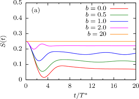
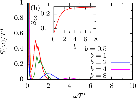
Figure 8: (color online) The spin correlation function $S(t)$ for increasing applied longitudinal fields (a), $N=18$ and an average over $n=10$ different configurations. (b) Corresponding calculated spectral functions $S(\omega)$. The inset depicts the spectral weight of the $\delta(\omega)$-peak as function of $b$ corresponding to the non-decaying fraction of $S(t)$. Parameter: $N_{C}=100$, $n=50$ and $r_{0}=1.5$.

Applying a magnetic field $B_{z}$ in longitudinal direction induces a finite energy difference between the different eigenstates of the total spin component $J_{z}$, and the spin-flip processes of the central spin are suppressed by this additional energy barrier. The initial spin-decay is almost independent of $b$ for ultra-short time scales until $t\approx 1/b$ where the further decay of $S(t)$ starts to be oppressed. Consequently, the non-decaying fraction of the spin polarization is increasing with $b$: the spin-decay is completely suppressed for $b\to\infty$ as can be seen in Fig. 8(a).

The corresponding spin-noise spectrum is displayed in Fig. 8(b). The increasing non-decaying fraction $S_{\infty}$ in $S(t)$ corresponds to an increasing spectral weight of the $\delta$-peak located at $\omega=0$. Since the total spectral weight is conserved, there is a spectral weight transfer from the broader peak centered around $\omega^{*}T^{*}\approx 1$ to the $\delta(\omega)$-peak. The broad finite-frequency peak is shifted to higher frequencies and is again centered at $\omega^{*}\approx\sqrt{b^{2}+1/2}$ at large magnetic field. The major difference to the application of a transversal magnetic field is the loss of spectral weight at finite frequencies in favor of the zero-frequency peak.

As discussed above, the CET is restricted to a finite accessible $t_{\rm max}\propto N_{C}$ which defines the lowest frequency resolution $\Delta\omega$. Therefore, the $\delta(\omega)$ cannot be accurately resolved. We define a low frequency cutoff $\omega_{\rm min}$ and calculate the total spectral weight $S_{+}$

$$S_{+} = \int_{\omega_{min}}^{\infty}\frac{d\omega}{2\pi}\,S(\omega)$$ (54)

of the finite frequency part of the spin-noise spectrum. Since the CET spin-noise exactly fulfills the spectral sum-rule, we obtain the spectral weight $S_{0}=2\pi S_{\infty}$ of the $\delta(\omega)$-peak from the difference $S_{0}=1/4-S_{+}$. The resulting $S_{\infty}$ as function of $b$ is plotted as inset in Fig. 8(b) and reveals the increase of the weight with increasing longitudinal magnetic field.

IV Spin dynamics of the anisotropic CSM

IV.1 Spin dynamics in the Ising limit

Up until now, the results were restricted to the isotropic case, $\lambda=1$. In order to set the stage for the anisotropic model with finite $\lambda<\infty$, we focus on the opposite limit $\lambda\rightarrow\infty$, the Ising limit, in this section. Then, the Hamiltonian (1) of the CSM reduces to an Ising interaction between the central spin and the nuclear spins

$$H =\omega_{L}\vec{S}\vec{n}_{B}+\sum_{k}A_{k}S^{z}I_{k}^{z}$$ (55)

and can be solved in a closed analytical form in some limiting cases.Koppens et al. (2007); Fischer et al. (2008); Testelin et al. (2009) This limit describes a pure heavy-hole spin.Koppens et al. (2007); Fischer et al. (2008); Testelin et al. (2009)

Obviously, all nuclear spin operators $I_{k}^{z}$ commute with $H$ and are conserved. Therefore, the spin-bath is static and fully determined by the eigenvalue configuration $\{m_{k}\}$ of all $I_{k}^{z}$. In the absence of an external magnetic field, the eigenenergies are given by $E^{*}(\sigma,\{m_{k}\})$

$$E^{*}(\sigma,\{m_{k}\}) = \sigma\sum_{k}A_{k}m_{k}=\sigma E^{*}\{m_{k}\})$$ (56)

where $\sigma$ is the eigenvalue of $S^{z}$.

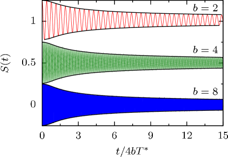
Figure 9: (color online) The spin noise function $S(t)$ for the Ising limit $\lambda\rightarrow\infty$ of the anisotropic central spin model plotted vs the dimensionless time $\tau=t/4bT^{*}$ for three values of the external magnetic field $b=2,4,8$. An offset of $0.5$ has been added to distinguish the three individual curves. The envelope of $E_{z}(\tau)$ given by Eq. (58) has been added as a black line to each simulation. All curves have been calculated for $r_{0}=1.5$, $n=20$ and $N=18$.

In a finite external magnetic field, the Hamilton matrix decomposes in $2\times 2$ subblocks for each fixed nuclear configuration $\{m_{k}\}$. For an external magnetic field in $x$-direction, we obtain the two eigenenergies $E_{\pm}(\{m_{k}\}))=\pm\sqrt{\omega_{L}^{2}+[E^{*}\{m_{k}\})]^{2}}/2$. The electronic spin precesses around the resulting effective magnetic field $\vec{B}_{\rm eff}(\{m_{k}\})=(\omega_{L},0,E^{*}(\{m_{k}\}))^{T}$ which depends on the bath configuration.Koppens et al. (2007)

Averaging over the Larmor oscillations, the projection of the spin component $\vec{n}[\vec{n}\vec{S}(0)]$ onto the magnetic field direction $\vec{n}$ survives as already discussed above in the context of Eq. (50). For a spin initially polarized in $z$-direction, the $z$-component of the non precessing contribution $(\vec{e}_{z}\vec{n})^{2}|\vec{S}(0)|$ has to be averaged over all nuclear configurations $\{m_{k}\}$

$$\left\langle(\vec{e}_{z}\vec{n})^{2}\right\rangle_{\{m_{k}\}} = \left\langle\frac{[E^{*}(\{m_{k}\})]^{2}}{\omega_{L}^{2}+[E^{*}\{m_{k}\})]^{2}}\right\rangle_{\{m_{k}\}}$$ (57)

where $\vec{e}_{z}$ is the unit vector in $z$-direction. For large magnetic fields, this average yields $\left\langle(\vec{e}_{z}\vec{n})^{2}\right\rangle=1/4b^{2}$ while in zero magnetic field $\left\langle(\vec{e}_{z}\vec{n})^{2}\right\rangle=1$.

When applying a transversal external magnetic field $B_{x}$, the fast dynamics of a spin initially polarized in $z$-direction is determined by the Larmor frequency $\omega_{L}\propto b$. The spin-decay, however, is governed by a slowly varying envelope function. Fig. 9 depicts the real-time dynamics of $S(t)$ for three values of a large external magnetic field for the Ising limit of the Hamiltonian. An offset of $0.5$ has been added to distinguish the different curves.

Testelin and collaboratorsTestelin et al. (2009) have extended the semi-classical approach of Merkulov et. al.Merkulov et al. (2002) to the Ising limit of the CSM and derived the analytic decay function $E_{z}(t)$

$$E_{z}(\tau) = \frac{1}{4}\left[\frac{\text{cos}(4b^{2}\tau+\frac{1}{2}\text{arctan}(\tau))}{(1+\tau^{2})^{1/4}}\right.$$ (58)

$$\left.+\frac{1}{4b^{2}}\left(1-\frac{\text{cos}(4b^{2}\tau+\frac{3}{2}\text{arctan}(\tau))}{(1+\tau^{2})^{3/4}}\right)\right],$$

for the spin-component in $z$-direction in the limit of large magnetic fields $b\gg 1$ where the new dimensionless time scale $\tau=t/4bT^{*}$ has been introduced. It consists of two oscillatory terms governed by the Larmor frequency $4b^{2}\tau=\omega_{L}t$ with an additional phase shift term and two decaying envelope functions $\propto(1+\tau^{2})^{1/4}$ and $\propto(1+\tau^{2})^{3/4}$. The functional form of this non-exponential decay has been derivedKoppens et al. (2007) by averaging the coherent spin-precession of the central spin for a given nuclear configuration $\{m_{k}\}$ over all nuclear configurations using a Gaussian distribution of the nuclear field. The value of the non-decaying fraction $1/4b^{2}$ agrees exactly with the prediction of Eq. (57). The increase of the dephasing time $T_{\rm deph}=4bT^{*}$ with increasing field strength can be understood by the suppression of the effective field fluctuation.

We have added the envelope of the function $E_{z}(\tau)$ to Fig. 9 for the three different magnetic field strengths. The semi-classical approach excellently reproduces the exact simulations for large magnetic fields $b\gg 1$. Our numerical results confirm the slow decay of the longitudinal spin component $\propto 1/\sqrt{t}$ for large times in this limit.

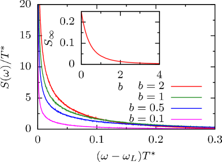
Figure 10: (color online) The spin noise spectra $S(\omega)$ for $(\omega-\omega_{L})\geq 0$ in the Ising limit calculated by exact Fourier transformation of (59) for different external magnetic fields $b$. The inset shows the non-decaying fraction $S_{\infty}$ which defines the spectral weight of the $\delta$-peak at $\omega=0$. Parameters: $N=18$, $r_{0}=1.5$.

While the power-law decay for large magnetic fields is well establishedKoppens et al. (2007); Fischer et al. (2008); Testelin et al. (2009) it is not obvious whether the analytic form of the long-time envelope prevails in the crossover regime to small fields. In order to reveal the envelope function for the long time decay, one can subtract the non-decaying fraction from $S(t)$ and multiply the remaining oscillatory part with the dominating long-time decay. We find that the amplitude of the oscillatory function $(S(t)-S_{\infty})(1+\tau^{2})^{1/4}$ reaches a time-independent long time limit – not shown here.

To substantiate these findings, we expand the initial spin polarized state $\left|\uparrow,\{m_{k}\}\right\rangle$

$$\left|\uparrow,\{m_{k}\}\right\rangle = c_{+}(\{m_{k}\})\left|+,\{m_{k}\}\right\rangle+c_{-}(\{m_{k}\})\left|-,\{m_{k}\}\right\rangle$$

using the exact eigenstates $\left|\pm,\{m_{k}\}\right\rangle$ for a given configuration $\{m_{k}\}$ and exactly calculate the spin-noise function $S(t)=\left\langle S^{z}(t)\right\rangle_{\rho_{p}}/2$ by averaging over all excitation energies $\Delta E(\{m_{k}\})=\sqrt{\omega_{L}^{2}+[E^{*}\{m_{k}\})]^{2}}$:

$$S(t) = S_{\infty}+\sum_{\{m_{k}\}}c_{+}^{2}c_{-}^{2}\cos(\Delta E(\{m_{k}\})t)$$ (59)

$$S_{\infty} = \sum_{\{m_{k}\}}\frac{1}{4}\left(c_{+}^{2}-c_{-}^{2}\right)^{2}\,\,.$$ (60)

While the time-independent part $S_{\infty}$ is equivalent to (57) and defines the spectral weight of $S(\omega)$ at zero frequency, the Fourier transformation of the second part can be calculated analytically and yields the exact finite frequency contribution to the noise spectra.

For the frequency distribution of $\sqrt{\omega_{L}^{2}+[E^{*}\{m_{k}\})]^{2}}$ we conclude that (i) there exists a finite threshold frequency $\omega_{\rm th}$ below which $S(0<\omega<\omega_{\rm th})=0$ and (ii) $\omega_{L}=\lim_{N\to\infty}\omega_{\rm th}$. Consequently, the spectral gap in $S(\omega)$ below $\omega_{\rm th}$ will prevail in the thermodynamic limit. Since the largest frequency in (59) is limited by the two fully polarized configurations $\{m_{k}=\uparrow\},\{m_{k}=\downarrow\}$, the spin noise spectrum $S(\omega)$ also must vanish for $|\omega|>\sqrt{\omega_{L}^{2}+[E^{*}_{\rm max}]^{2}}$.

Fig. 10 depicts the exact $S(\omega)$ as function of $\omega-\omega_{L}$ for different magnetic fields. $S(\omega)$ can be fitted by a power law $(\omega-\omega_{L})^{-\alpha}$ very close to the Larmor frequency. We have extracted a universal exponent $\alpha\approx 1/2$ independent of $b$. For small $b$, however, the non-decaying fraction of the spin dominates and the finite frequency spectral function is very small. Therefore, the fitting accuracy decreases for $b\to 0$.

Approximating $S(\omega)$ by $C(\omega-\omega_{L})^{-\alpha}$ close to the threshold frequency up to some finite cutoff frequency $\omega_{\rm max}$ and a normalization constant $C$, we can analytically extrapolate the long-time approach to $S_{\infty}$ from

$$\Delta S(t) = S(t)-S_{\infty}=2\Re e\left[\int_{\omega_{L}}^{\omega_{\rm max}}\frac{d\omega}{2\pi}\frac{C}{(\omega-\omega_{L})^{\alpha}}e^{i\omega t}\right]$$ (61)

$$= \frac{C}{\pi t^{1-\alpha}}\Re e\left[e^{i\omega_{L}t}\int_{0}^{(\omega_{\rm max}-\omega_{L})t}du\frac{e^{iu}}{u^{\alpha}}\right]$$

which can be approximated for $t\to\infty$ and $\alpha=1/2$ to

$$\Delta S(t) \approx \frac{aC}{\pi}\frac{\cos(\omega_{L}t+\pi/4)}{\sqrt{t}}$$ (62)

where $a\approx 1.25331$. This result recovers the long-term limit of $E_{z}(t)$ stated in Eq. (58) independent from the $b\gg 1$ limit.

IV.2 Spin dynamics in the generic anisotropic CSM

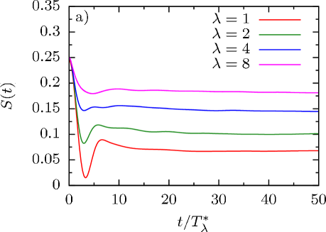
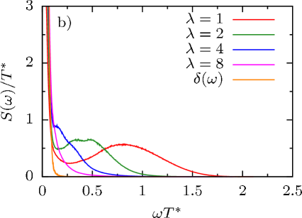
Figure 11: (color online) (a) $S(t)$ vs $t/T^{*}_{\lambda}$ for different values of the anisotropy factor $\lambda=1,2,4,8$. (b) Spin-noise spectra vs $\omega T^{*}$ for the same parameters as in panel (a) and $N_{C}=100$. A $\delta$-peak at zero frequency resolved by the CET with the same number of moments has been added as reference. Parameters: $N=18,n=50,r_{0}=1.5$.

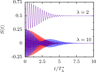
Figure 12: (color online) Comparison between the analytical prediction (blue) of Eq (26c) of Ref. [Testelin et al., 2009] using a QSA and the CET approach for $b/\lambda>1$. All curves have been calculated for $b=10$ and $\lambda=2$ or $\lambda=10$. We have added an offset of $0.5$ to the $\lambda=2$-curves for better comparison. Parameters: $N=18,r_{0}=1.5$.

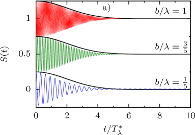
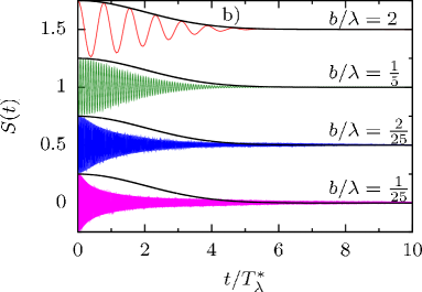
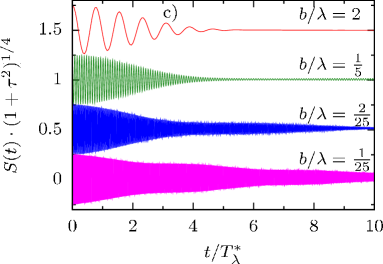
Figure 13: (color online) $S(t)$ in a transversal magnetic field: (a) for a fixed value $\lambda=10$ and $b=2,6,10$, and (b) for a fixed value $b=4$ and four different values of $\lambda=2,20,50,100$. For all cases we have added the envelope function $0.25\exp[-(t/T^{*}_{\lambda})^{2}/8]$ to reveal the difference to the short-time dynamics of the isotropic CSM. (c) Rescaled spin correlation function $S(t)(1+\tau^{2})^{1/4}$ vs $t/T^{*}_{\lambda}$ for the same parameters as in panel (b) with $\tau=t/4bT^{*}_{1}$. Parameters: $N=18,n=20,r_{0}=1.5$.

So far we have discussed the two extreme limits of the Hamiltonian (1): the isotropic CSM and the Ising limit. Now we investigate the influence of an arbitrary anisotropy factor $\lambda$ onto the spin-noise spectra as function of a transversal external magnetic field.

In the absence of an external magnetic field, the decay of the spin correlation function $S(t)$ is only caused by the transversal terms in the Hamiltonian whose relative strength is controlled by the factor $1/\lambda$. Presenting the data as function of the dimensionless time $t/T^{*}_{\lambda}=t/\lambda T^{*}$ clearly reveals the $\lambda$-dependence of the intrinsic time scale: the location of the minimum in the short-time dynamics remains almost independent of $\lambda$ as depicted in Fig. 11(a). With increasing $\lambda$, the non-decaying fraction of $S(t)$ monotonically increases, and the curves basically interpolate between the isotropic CSM limit and Ising limit where $S(t)=1/4=const.$ does not decay at all.

The corresponding spin-noise spectrum $S(\omega)$ is shown as a function of the dimensionless frequency $\omega T^{*}_{1}$ in Fig. 11(b). We have added the result for the isotropic CSM as reference for comparison. Since the CET approach has a finite resolution of a $\delta(\omega)$-peak for $\omega\to 0$, the data for $\lambda=\infty$ serves as reference and indicates the change of the spectral function at finite frequencies as function of $\lambda$. The height of the Gaussian shaped peak close to $\omega\approx 1/T^{*}_{\lambda}$ of the isotropic CSM decreases with increasing $\lambda$, and spectral weight is shifted in parts into the $\delta$-peak at $\omega=0$ and to smaller frequencies $\omega>0$. For $\lambda>3$, the peak close to $\omega\approx 1/T^{*}_{\lambda}$ has disappeared and the spectra are monotonically increasing for decreasing $\omega$.

Now we proceed to the spin response in a transversal magnetic field. A word is in order to clarify the definition of a strong external field in the anisotropic CSM. The Hamiltonian (1) contains two terms driving (i) the decoherence and (ii) the dephasing of the central spin in $z$-direction: (i) the transversal spin-flip term is governed by the characteristic timescale $T^{*}_{\lambda}$ and (ii) the external transversal field is governed by $T^{*}_{\lambda}/\lambda b$. If $b\cdot\lambda\gg 1$ holds, the external magnetic field dominates over the spin-flip term, and, therefore, is called a strong external field. The central spin performs several Larmor precessions before the decoherence due to the nuclei sets in to the spin bath. In the opposite limit, $b\cdot\lambda\ll 1$, the central spin cannot complete a single Larmor precession on the time scale $T^{*}_{\lambda}$ on which $S(t)$ decays due to the hyperfine interaction.

We begin to investigate the strong field regime defined by $b\cdot\lambda>1$. We compare the analytical predictionsTestelin et al. (2009) by the QSA with our CET results for short-time and intermediate-time scales as depicted in Fig. 12. While for $\lambda=2,b=10$ good agreement is found between both methods significant deviations are observed for an increased asymmetry $\lambda=10,b=10$ already at short times. While the numerical exact results show a monotonic decay of the envelope function, the QSA predicts an oscillation of the spin polarization amplitude. It turns out that this result can be generalized to the statement, that Eq (26c) of Ref. [Testelin et al., 2009] using the QSA only describes $S(t)$ in a transversal magnetic field adequately if the parameter $b/\lambda$ is large compared to $1$. This indicates the importance of the ratio $b/\lambda$ for separating different types of the dynamics in the anisotropic central spin model.

To gain more information on the influence of the ratio $b/\lambda$, CET results for $S(t)$ are shown at either a fixed $\lambda=10$ and different magnetic field strengths $b=2,6,10$ in panel (a), or at fixed magnetic field strength $b=4$ and several values of $\lambda=2,10,20,50$ in panel (b) of Fig. 13. Augmenting the numerical data with the envelope funtion $0.25\exp[-(t/T^{*}_{\lambda})^{2}/8]$ demonstrates that the short-time response is governed by the characteristic time scale $T^{*}_{\lambda}$ and the decay is well captured by a Gaussian envelope function for $b/\lambda\geq 1$ as predicted by the QSA.Testelin et al. (2009)

Deviations from such a Gaussian decay increase with decreasing ratio $b/\lambda<1$ and are very pronounced for $b/\lambda=1/25$. For these parameters, the initial decay occurs much faster but on long-time scales significantly slower than described by a Gaussian envelope function. The dependency of the crossover on the ratio $b/\lambda$ can be understood from the fact that the hyperfine-field asymmetry increases with increasing $\lambda$, and a larger transversal external magnetic field $b$ is required to induce a dynamics similar to the isotropic CSM. Only at very strong transversal magnetic fields $B_{x}$, the relevance of anisotropy of the hyperfine interaction is reduced and the Gaussian type of decay is expected for $b/\lambda>1$.

For strong external fields, $b\cdot\lambda>1$, the ratio $b/\lambda$ solely dictates the form of the envelope of $S(t)$: for several different combinations of $b$ and $\lambda$, the envelope functions for $S(t)-S_{\infty}$ are identical - being not explicitly shown here.

For further illustration of the crossover from a Gaussian to the Ising type decay, we plotted the rescaled spin correlation function $S(t)[1+\tau^{2}]^{1/4}$ vs $t/T^{*}_{\lambda}$ in Fig. 13(c), where $\tau=t/4bT^{*}$. This reveals an Ising type power law decay for long-time scales that is recovered for $\lambda\to\infty$. For $b=4$ and $b/\lambda=2$, we clearly observe a Gaussian dominated decay. For decreasing $b/\lambda$, an increasing intermediate-time regime develops where the envelope function follows a slower power-law type decay. Note that $S(t)[1+\tau^{2}]^{1/4}$ yields a non-decaying oscillation in the Ising limit, which can not be shown in figure 13(c) due to the underlying time-scale.

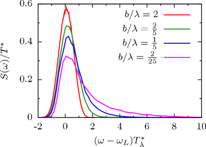
Figure 14: (color online) Spin noise spectra $S(\omega)$ for $b=4$ and $\lambda=2,10,20,50$, plotted vs $(\omega-\omega_{L})T^{*}_{\lambda}$. Since the characteristic time-scale $T^{*}_{\lambda}$ increases with increasing $\lambda$, we adjusted the number of Chebychev momenta to $N_{C}(\lambda=2)=100$, $N_{C}(\lambda=10)=300$, $N_{C}(\lambda=20)=600$, and $N_{C}(\lambda=50)=1500$ to provide an adequate frequency resolution. The chosen parameters are equivalent to those in FIG. 13.

We have been able to identify three different regimes for $b\cdot\lambda>1$. For $b>\lambda$, (i) the decay is of Gaussian typeTestelin et al. (2009) similar to the isotropic CSM. As long as $\lambda$ is less than one order of magnitude larger than $b$, (ii) the decay of $S(t)$ deviates from the Gaussian envelope, but the long-time decay is still governed by the tail of the envelope function. In the last regime, (iii) where $\lambda\gg b$ holds, the behavior of the spin-noise function approaches the Ising regime discussed in the previous section.

The corresponding spin-noise spectrum for this crossover regime $b/\lambda<1$ is depicted as function of $(\omega-\omega_{L})T_{\lambda}^{*}$ in Fig. 14. In leading order, the peak position of $S(\omega)$ is clearly given by the Larmor frequency $\omega_{L}$, while the peak width is governed by $T^{*}_{\lambda}$. Note that the smallest and the largest value of $\lambda$ differ by a factor of $25$. Therefore, the increase of $T^{*}_{\lambda}$ requires a significant increase of the Chebychev order $N_{C}$ for a reliable resolution of the spectra. $S(\omega)$ evolves from a Gaussian shape for $b/\lambda=2$, to a precursor of a threshold behavior for $b/\lambda=2/25$. While the high frequency tail can be fitted with a Lorentzian, the low frequency spectrum is rapidly suppressed below the Larmor frequency for $0<\omega<\omega_{L}$ with increasing anisotropy. In the limit $\lambda\to\infty$, the Ising limit of the spectrum, as shown in Fig. 10, must be recovered. Therefore, the increasing low frequency gap with increasing asymmetry prevails in the thermodynamic limit.

Let us now turn to small magnetic fields characterized by the condition $b\cdot\lambda\ll 1$. In this case the central spin experiences decoherence induced by the spin bath before a whole Larmor precession can occur. The short-time dynamics in this regime is governed by $T^{*}_{\lambda}$ and is of the same form as shown for different values of $\lambda$ in Fig. 11(a). After the initial spin decay, $S(t)$ will approach zero on a large timescale that is dictated by $\lambda/\omega_{L}$. This long-time behavior of $S(t)$ is analogous to the isotropic CSM as shown in Fig. 7(b). Combining the information provided by both figures fully describes the long-time and short-time behavior of $S(t)$ in the weak field limit of the anisotropic CSM, and we do not show further explicit results for this regime.

So far we did not discuss the correlation function $S(t)$ for a light hole spin. Such QDs are characterized by an anisotropy factor $\lambda=1/2<1$, so that the spin-flip terms dominate over the Ising contribution. Since $b/\lambda>1/\lambda^{2}>1$ is bound in the strong field regime, no Ising-type behavior can be observed and $S(t)$ always shows a Gaussian type decay for $b\cdot\lambda>1$. However, all other findings discussed above remain valid for the case $\lambda<1$: an analogous behavior for the weak field limit $b\cdot\lambda\ll 1$ is found. Overall, the spin noise is very similar to the isotropic CSM but with a faster characteristic time scale $T^{*}\to T^{*}_{\lambda}<T^{*}$.

V Spin noise spectra in quantum dot ensembles

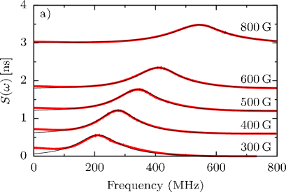
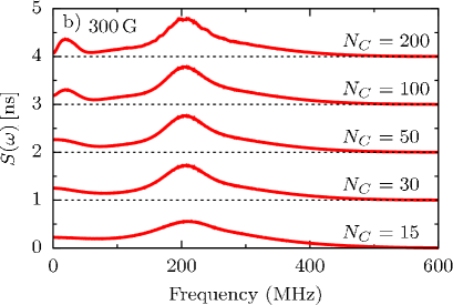
Figure 15: (color online) (a) Ensemble averaged spin-noise spectra vs $\omega$ for five different values of $B$ for a dot-confined electron spin, i. e. $\lambda=1$. Defining the average timescale $\overline{T}^{*}=\left\langle T^{*}\right\rangle=1$ ns as reference, and using $|g_{e}|=0.54$ as in Ref. Crooker et al., 2010, $S(\omega)$ has been obtained by averaging over $n=100$ different spectra generated from a constant distribution of $T^{*}\in[0.2\,{\rm ns},1.8\,{\rm ns}]$ of characteristic single QD time scales. For better visibility, an offset proportional to $b=\omega_{L}\overline{T}^{*}$ has been added to $S(\omega)$. Parameters: $N_{C}=15,N=18$. The black lines indicate Lorentzian fits to the individual curves. (b) Evolution of the ensemble noise spectrum with increasing $N_{C}$ at fixed $B=300$ G.

The spin noise spectrum has been measuredCrooker et al. (2010); Dahbashi et al. (2012); Li et al. (2012); *ZapasskiiGreilichBayer2013 on QD ensembles charged with a single electron or hole. To bridge between the single QD calculations and the recent experiments, we have performed an ensemble average of $n$ single independent QD spectra with different configurations $\{A_{k}\}$. We have used the average timescale $\overline{T^{*}}=\left\langle T^{*}\right\rangle$ as reference timescale with equally distributed individual $T^{*}\in[0.2\overline{T^{*}},1.8\overline{T^{*}}]$ for each individual QD.

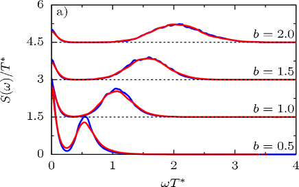
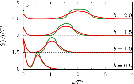
Figure 16: (color online) (a) Ensemble averaged spin-noise spectra in the asymmetric CSM for $\lambda=5$ (red) and $\lambda=50$ (blue) for different $b$. $S(\omega)$ has been obtain by averaging over $n=2000$ different single QD spectra generated from a constant distribution of $T^{*}_{i}\in[0.2T^{*},1.8T^{*}]$, and the individual $g$ factors are taken from a Gaussian distribution with $\Delta g/g=0.2$. (b) Influence of the $g$-factor distribution function on the shape of the spin-noise spectrum: comparing the $\lambda=5$ data of (a) with an ensemble averaged $S(\omega)$ where the individual $g$ factors $g_{i}$ are taken from a constant distribution of $g_{i}/g\in[0.8,1.2]$ (green curves). For better visibility, an offset proportional to $b$ has been added to $S(\omega)$. Parameters: $N=18,N_{C}=50,r_{0}=1.5$.

For QD ensembles with dot-confined electrons the distribution of $g$-factors is very sharp,Greilich et al. (2007) and the spread of the $g$ factors can be neglected. The resulting ensemble averaged spin-noise spectra are depicted in Fig. 15(a). An offset proportional to the magnetic field $b$ has been added to $S(\omega)$ for better visibility. The black lines indicate a Lorentzian fit to each individual curve.

For the absolute units in Fig. 15, we have set the average electron dephasing time $\overline{T^{*}}=1\,\text{ns}$ and have used the experimentally determinedCrooker et al. (2010) electron $g$-factor $|g_{e}|=0.54$. Our results demonstrate that phenomenological Lorentz fits to the experimental spin noise spectra are justified for strong external magnetic fields $b=\omega_{L}\overline{T^{*}}>1$. For small $b$ significant deviations from a simple Lorentzian fit are observed in the ensemble averaged spectra as being reported in the experimental data.Crooker et al. (2010) These deviations are related to the low-frequency features of the spin-noise ignored in such a simple Lorentzian fit.

Our results are in good agreement with the experimental data of Fig. 4(a) in Ref. Crooker et al., 2010. For larger Chebyshev orders the ensemble averaging still provides peaks around the Larmor-frequency in $S(\omega)$ that can be approximated by a Lorentzian, but a clear gap between zero frequency and $\omega_{L}$ occurs as discussed before.

Note that the spectra presented in Fig. 15(a) have been calculated for a relatively small Chebyshev order $N_{C}=15$ corresponding to a frequency resolution of $\omega>20$ MHz for a magnetic field of $B=300$ G up to $\omega>60$ MHz for $B=800$ G. This would mimic a limited resolution in the experiments.

The effect of an increase of the frequency resolution (increasing $N_{C}$) on the spectral properties of the ensemble averaged spin noise is depicted in Fig. 15(b) for a fixed magnetic field $B=300$ G. While the broadened peak around $200$ MHz converges very quickly by a small amount of narrowing, the additional low-frequency feature can now be resolved. This would apply to all spectra shown in 15(a): the additional frequency resolution does not change the qualitative properties of the spin noise in a transverse magnetic field but only reveals additional spectral information at low frequency.

Now we turn to hole spin ensembles modeled by the anisotropic CSM. In this case the distribution of the $g$-factors in the QDs is crucial when making connection to measurementsLi et al. (2012); *ZapasskiiGreilichBayer2013 of spin noise in those QD ensembles. To account for this spread, we have used a Gaussian probability distribution for the $g$-factors centered at $g$ with standard deviation $\Delta g/g=0.2$ to include a random value of $g$ for each individual QD in our simulations. In addition, the average dephasing time $\overline{T^{*}}=\left\langle T^{*}\right\rangle$ is set as reference time (and reciprocal energy) scale, and the individual time scales $T^{*}$ have been generated from a constant distribution $T^{*}\in[0.2T^{*},1.8T^{*}]$ for each of the $n=2000$ individual QD calculations entering the ensemble average. The resulting averaged $S(\omega)$ are depicted in Fig. 16(a) for two different values of $\lambda=5,50$.

It is striking that the width of the ensemble averaged $S(\omega)$ hardly depends of the anisotropy factor $\lambda$, although the peak width is given by $1/T^{*}_{\lambda}=1/\lambda T^{*}$ in a single QD. In a QD ensemble of hole spins, however, the peak width of the noise spectra is determined by the distribution of $g$-factors, and, consequently, the spectral width of $S(\omega)$ increases with increasing external magnetic field.

To illustrate the influence of the $g$-factor distribution function onto the shape of ensemble averaged $S(\omega)$, we have combined the $\lambda=5$ spectra of Fig. 16(a) with another set of ensemble averaged $S(\omega)$ calculated by using a constant distribution function $b_{i}/b\in[0.8,1.2]$ but otherwise identical parameters (green curves) in Fig. 16(b). Clearly, the peak shape of $S(\omega)$ obtained from a box-shaped $g$-factor distribution function resembles strongly this distribution function while the spectra of Fig. 16(a) (red curves) exhibit a more Gaussian-type shape.

As a consequence, the shape of ensemble averaged spin-noise spectra is mainly governed by the two distribution functions for $g$ and $T^{*}$ and reveal less information about the dephasing mechanism in a single quantum dot. Therefore, it would be desirable to be able to measure the spin noise directly on a single quantum dot in order to obtain additional information on the microscopic dephasing mechanism of an electron or hole spin in a QD.

VI Discussion and outlook

We have presented a comprehensive study of the spin-noise in the minimal model for dephasing in QDs, the anisotropic CSM. We have investigated the dependency of $S(t)$ and its Fourier transform $S(\omega)$ on the external magnetic field and the anisotropy parameter $\lambda$ using a CET approach. This approach provides a time-evolution of an arbitrary initial state whose error can be reduced to machine precision for any give time $t$. We have extended the CET to ensemble averaging of traces needed to account for a fully incoherent spin-bath.

In the absence of an external magnetic field, $S(t)$ exhibits an universal time evolution for the isotropic CSM on a very short time scale governed by the bath-spin fluctuation time $T^{*}$. At intermediate times $t/T^{*}<100$, the dynamics depend on the distribution function of the hyperfine coupling constants. While a semi-classical approximation predicts a finite non-decaying fraction of the spin polarization of $S^{\text{QSA}}_{\infty}=S(0)/3$ by averaging over a distribution of static nuclear field configurations, our CET results are typically below $S^{\text{QSA}}_{\infty}$. Fluctuations of the nuclear spin bath occur on a much longer time scale and can lead to significant deviations from the quasi-static approximation when the hyperfine coupling constants cover a large parameter range. Typically we find a very slow decay at intermediate and long-time scales driven by the distribution of the small hyperfine interaction constants $A_{k}$. Finite size scaling of the non-decaying fraction of the spin polarization of $S_{\infty}$ as function of the cutoff $r_{0}$ indicates vanishing $S_{\infty}$ in the thermodynamic limit in agreement with the intuitive but not rigorous argument of Chen et al.Chen et al. (2007)

For the isotropic CSM, we find that the spin-noise spectrum consists of three parts: (i) a zero-frequency $\delta$-peak whose spectral weight is given by the non-decaying fraction of the central spin, (ii) a low-frequency threshold behavior which follows approximately a power-law and is cut off at the smallest non-zero excitation energy of the finite-size system determined by $\bar{A}_{\rm min}(r_{0})$ and (iii) a Gaussian-type high frequency peak around $\omega T^{*}\approx 1$ which determines the short time dynamics on time scales of $T^{*}$. We find a remarkable agreement with a $\omega^{-3/4}$ fit to the low-frequency part of our high resolution CET spin-noise spectrum which suggests an asymptotic $1/t^{1/4}$ spin-decay at long times which is not contradicting the approximative solutions in the literature: on intermediate time scales $1/t^{1/4}$ and $1/\log(t)^{3/2}$ are nearly indistinguishable and only deviate significantly in their asymptotic behavior. We conjecture that in the thermodynamic limit the zero-frequency $\delta$-peak will disappear, and the low-frequency spectra will show a pronounced threshold behavior which will govern the long-time spin-decay. For a detailed analysis of its analytical form, other approaches have to be employed.

The Ising limit of the CSM is exactly solvable by treating the $2\times 2$ Hamiltonian subspaces for each frozen nuclear spin configuration leading to a strict threshold behavior of the noise spectra. The spectrum consists of a $\delta(0)$ peak whose spectral weight decreases with increasing $b$ and close to the threshold a $\omega^{-1/2}$ fit can be applied to the data, yielding a $t^{-1/2}$ long time decay independently of the applied magnetic field. In the Ising limit pure dephasing occurs and we find that an increase of the external field yields an increasing coherence time of the central spin due to the decreasing spread of the eigenenergies.

In the anisotropic CSM without an external magnetic field the timescale $T^{*}_{\lambda}$ determines the short-time evolution of the central spin. We have demonstrated that in a transversal magnetic field the value of $b\cdot\lambda$ separates hyperfine interaction driven spin dynamics from magnetic field dominated spin dynamics. For $b\cdot\lambda>1$, the ratio $b/\lambda$ describes the crossover from Ising-like dynamics ($b/\lambda\ll 1$) to a more Gaussian type decay ($b/\lambda>1$.) For a single QD in a strong external field we always find a clear energy gap in the spin-noise between $\omega=0$ and the broadened peak close to the Larmor frequency whose width is given by $1/T^{*}_{\lambda}$.

Furthermore, we have performed an ensemble average of the spin-noise spectra to compare our calculations to recent spin-noise measurements on QD ensembles. By using realistic characteristic time scales $T^{*}$, the experimentally determined distribution of $g$-factors, we find qualitative agreement for QD ensembles of both hole spins and electron spins. Our calculations reveal the shape dependence of ensemble averaged noise spectra on the distribution functions for the $g$-factors and the characteristic time scales $T^{*}$: the averaged noise spectrum contains less information on the dephasing mechanism than the data for an individual quantum dot.

We acknowledge fruitful discussions with Manfred Bayer, Scott Crooker, Alex Greilich, Nikolai Sinitsyn, Joachim Stolze, Götz Uhrig, and Dmitri Yakovlev.

References

- Schliemann et al. (2003) J. Schliemann, A. Khaetskii, and D. Loss, Journal of Physics: Condensed Matter 15, R1809 (2003).
- Hanson et al. (2007) R. Hanson, L. P. Kouwenhoven, J. R. Petta, S. Tarucha, and L. M. K. Vandersypen, Rev. Mod. Phys. 79, 1217 (2007).
- Elzerman et al. (2004) J. M. Elzerman, R. Hanson, L. H. W. van Beveeren, B. Witkamp, L. M. K. Vandersypen, and L. P. Kouvenhoven, Nature 430, 431 (2004).
- Bonadeo et al. (1998) N. H. Bonadeo, J. Erland, D. Gammon, D. Park, D. S. Katzer, and D. G. Steel, Science 282, 1473 (1998) .
- Greilich et al. (2007) A. Greilich, A. Shabaev, D. R. Yakovlev, A. L. Efros, I. A. Yugova, D. Reuter, A. D. Wieck, and M. Bayer, Science 317, 1896 (2007).
- Fokina et al. (2010) L. V. Fokina, I. A. Yugova, D. R. Yakovlev, M. M. Glazov, I. A. Akimov, A. Greilich, D. Reuter, A. D. Wieck, and M. Bayer, Phys. Rev. B 81, 195304 (2010).
- Spatzek et al. (2011) S. Spatzek, A. Greilich, S. E. Economou, S. Varwig, A. Schwan, D. R. Yakovlev, D. Reuter, A. D. Wieck, T. L. Reinecke, and M. Bayer, Phys. Rev. Lett. 107, 137402 (2011).
- Merkulov et al. (2002) I. A. Merkulov, A. L. Efros, and M. Rosen, Phys. Rev. B 65, 205309 (2002).
- Khaetskii et al. (2003) A. Khaetskii, D. Loss, and L. Glazman, Phys. Rev. B 67, 195329 (2003).
- Coish and Loss (2004) W. A. Coish and D. Loss, Phys. Rev. B 70, 195340 (2004).
- Fischer et al. (2008) J. Fischer, W. A. Coish, D. V. Bulaev, and D. Loss, Phys. Rev. B 78, 155329 (2008).
- Testelin et al. (2009) C. Testelin, F. Bernardot, B. Eble, and M. Chamarro, Phys. Rev. B 79, 195440 (2009).
- Gaudin (1976) M. Gaudin, J. Physique 37, 1087 (1976).
- Andrei et al. (1983) N. Andrei, K. Furuya, and J. H. Lowenstein, Rev. Mod. Phys. 55, 331 (1983).
- Bortz and Stolze (2007) M. Bortz and J. Stolze, Phys. Rev. B 76, 014304 (2007).
- Bortz et al. (2010) M. Bortz, S. Eggert, and J. Stolze, Phys. Rev. B 81, 035315 (2010).
- Faribault and Schuricht (2013a) A. Faribault and D. Schuricht, Phys. Rev. Lett. 110, 040405 (2013a).
- Faribault and Schuricht (2013b) A. Faribault and D. Schuricht, Phys. Rev. B 88, 085323 (2013b).
- Crooker et al. (2010) S. A. Crooker, J. Brandt, C. Sandfort, A. Greilich, D. R. Yakovlev, D. Reuter, A. D. Wieck, and M. Bayer, Phys. Rev. Lett. 104, 036601 (2010).
- Dahbashi et al. (2012) R. Dahbashi, J. Hübner, F. Berski, J. Wiegand, X. Marie, K. Pierz, H. W. Schumacher, and M. Oestreich, Appl. Phys. Lett. 100, 031906 (2012).
- Li et al. (2012) Y. Li, N. Sinitsyn, D. L. Smith, D. Reuter, A. D. Wieck, D. R. Yakovlev, M. Bayer, and S. A. Crooker, Phys. Rev. Lett. 108, 186603 (2012).
- Zapasskii et al. (2013) V. S. Zapasskii, A. Greilich, S. A. Crooker, Y. Li, G. G. Kozlov, D. R. Yakovlev, D. Reuter, A. D. Wieck, and M. Bayer, Phys. Rev. Lett. 110, 176601 (2013).
- Ezer and Kosloff (1984) H. Tal-Ezer and R. Kosloff, J. Chem. Phys 81, 3967 (1984).
- Kosloff (1994) R. Kosloff, Ann. Rev. Phys. Chem. 45, 145 (1994).
- Weiße et al. (2006) A. Weiße, G. Wellein, A. Alvermann, and H. Fehske, Rev. Mod. Phys. 78, 275 (2006).
- Dobrovitski and De Raedt (2003) V. V. Dobrovitski and H. A. De Raedt, Phys. Rev. E 67, 056702 (2003).
- Zhang et al. (2006a) W. Zhang, V. V. Dobrovitski, K. A. Al-Hassanieh, E. Dagotto, and B. N. Harmon, Phys. Rev. B 74, 205313 (2006a).
- Yuan et al. (2008) S. Yuan, M. I. Katsnelson, and H. De Raedt, Phys. Rev. B 77, 184301 (2008).
- Yoshida et al. (1990) M. Yoshida, M. A. Whitaker, and L. N. Oliveira, Phys. Rev. B 41, 9403 (1990).
- Bulla et al. (2008) R. Bulla, T. A. Costi, and T. Pruschke, Rev. Mod. Phys. 80, 395 (2008).
- Anders and Schiller (2005) F. B. Anders and A. Schiller, Phys. Rev. Lett. 95, 196801 (2005).
- Anders and Schiller (2006) F. B. Anders and A. Schiller, Phys. Rev. B 74, 245113 (2006).
- Leggett et al. (1987) A. J. Leggett, S. Chakravarty, A. T. Dorsey, and M. P. A. Fisher, Rev. Mod. Phys. 59, 1 (1987).
- Erlingsson and Nazarov (2004) S. I. Erlingsson and Y. V. Nazarov, Phys. Rev. B 70, 205327 (2004).
- Cucchietti et al. (2005) F. M. Cucchietti, J. P. Paz, and W. H. Zurek, Phys. Rev. A 72, 052113 (2005).
- Merkulov et al. (2010) I. A. Merkulov, G. Alvarez, D. R. Yakovlev, and T. C. Schulthess, Phys. Rev. B 81, 115107 (2010).
- Al-Hassanieh et al. (2006) K. A. Al-Hassanieh, V. V. Dobrovitski, E. Dagotto, and B. N. Harmon, Phys. Rev. Lett. 97, 037204 (2006).
- Chen et al. (2007) G. Chen, D. L. Bergman, and L. Balents, Phys. Rev. B 76, 045312 (2007).
- Sinitsyn et al. (2012) N. A. Sinitsyn, Y. Li, S. A. Crooker, A. Saxena, and D. L. Smith, Phys. Rev. Lett. 109, 166605 (2012).
- Glazov and Ivchenko (2012) M. M. Glazov and E. L. Ivchenko, Phys. Rev. B 86, 115308 (2012).
- Stanek et al. (2013) D. Stanek, C. Raas, and G. S. Uhrig, Phys. Rev. B 88, 155305 (2013).
- White (1992) S. R. White, Phys. Rev. Lett. 69, 2863 (1992).
- Schollwöck (2005) U. Schollwöck, Rev. Mod. Phys. 77, 259 (2005).
- Schollwöck (2011) U. Schollwöck, Annals of Physics 326, 96 (2011).
- Friedrich (2006) A. Friedrich, Time-dependent Properties of one-dimensional Spin-Systems: a DMRG-Study, Ph.D. thesis, RWTH Aachen (2006).
- Lee et al. (2005) S. Lee, P. von Allmen, F. Oyafuso, G. Klimeck, and K. B. Whaley, J. Appl. Phys. 97, 043706 (2005).
- Abragam (1961) A. Abragam, The Principles of Nuclear Magnetism (Oxford U.P., 1961).
- Abramowitz and Stegun (1972) M. Abramowitz and I. A. Stegun, eds., Handbook of mathematical Functions (Dover Publications, 1972).
- Khaetskii et al. (2002) A. V. Khaetskii, D. Loss, and L. Glazman, Phys. Rev. Lett. 88, 186802 (2002).
- Zhang et al. (2006b) W. Zhang, V. V. Dobrovitski, K. A. Al-Hassanieh, E. Dagotto, and B. N. Harmon, Phys. Rev. B 74, 205313 (2006b).
- Koppens et al. (2007) F. H. L. Koppens, D. Klauser, W. A. Coish, K. C. Nowack, L. P. Kouwenhoven, D. Loss, and L. M. K. Vandersypen, Phys. Rev. Lett. 99, 106803 (2007).