\@IEEEtunefonts

Quasi-Static Multiple-Antenna Fading Channels at Finite Blocklength

Wei Yang, , Giuseppe Durisi, ,
Tobias Koch, , and Yury Polyanskiy
This work was supported in part by the Swedish Research Council under grant 2012-4571, by the Ericsson Research Foundation under grant FOSTIFT-12:022, by a Marie Curie FP7 Integration Grant within the 7th European Union Framework Programme under Grant 333680, by the Spanish government (TEC2009-14504-C02-01, CSD2008-00010, and TEC2012-38800-C03-01), and by the National Science Foundation under Grant CCF-1253205. The material of this paper was presented in part at the 2013 and 2014 IEEE International Symposium on Information Theory.W. Yang and G. Durisi are with the Department of Signals and Systems, Chalmers University of Technology, 41296, Gothenburg, Sweden (e-mail: {ywei, durisi}@chalmers.se).T. Koch is with the Signal Theory and Communications Department, Universidad Carlos III de Madrid, 28911, Leganés, Spain (e-mail: koch@tsc.uc3m.es).Y. Polyanskiy is with the Department of Electrical Engineering and Computer Science, MIT, Cambridge, MA, 02139 USA (e-mail: yp@mit.edu).
Abstract

This paper investigates the maximal achievable rate for a given blocklength and error probability over quasi-static multiple-input multiple-output (MIMO) fading channels, with and without channel state information (CSI) at the transmitter and/or the receiver. The principal finding is that outage capacity, despite being an asymptotic quantity, is a sharp proxy for the finite-blocklength fundamental limits of slow-fading channels. Specifically, the channel dispersion is shown to be zero regardless of whether the fading realizations are available at both transmitter and receiver, at only one of them, or at neither of them. These results follow from analytically tractable converse and achievability bounds. Numerical evaluation of these bounds verifies that zero dispersion may indeed imply fast convergence to the outage capacity as the blocklength increases. In the example of a particular $1\times 2$ single-input multiple-output (SIMO) Rician fading channel, the blocklength required to achieve $90\%$ of capacity is about an order of magnitude smaller compared to the blocklength required for an AWGN channel with the same capacity. For this specific scenario, the coding/decoding schemes adopted in the LTE-Advanced standard are benchmarked against the finite-blocklength achievability and converse bounds.

I Introduction

Consider a delay-constrained communication system operating over a slowly-varying fading channel. In such a scenario, it is plausible to assume that the duration of each of the transmitted codewords is smaller than the coherence time of the channel, so the random fading coefficients stay constant over the duration of each codeword [1, p. 2631],[2, Sec. 5.4.1]. We shall refer to this channel model as quasi-static fading channel.111The term “quasi-static” is widely used in the communication literature (see, e.g., [2, Sec. 5.4.1],[3]). The quasi-static channel model belongs to the general class of composite channels [1, p. 2631],[4] (also known as mixed channels [5, Sec. 3.3]).

When communicating over quasi-static fading channels at a given rate $R$, the realization of the random fading coefficient may be very small, in which case the block (frame) error probability $\epsilon$ is bounded away from zero even if the blocklength $n$ tends to infinity. In this case, the channel is said to be in outage. For fading distributions for which the fading coefficient can be arbitrarily small (such as for Rayleigh, Rician, or Nakagami fading), the probability of an outage is positive. Hence, the overall block error probability $\epsilon$ is bounded away from zero for every positive rate $R>0$, in which case the Shannon capacity is zero. More generally, the Shannon capacity depends on the fading probability density function (pdf) only through its support [6, 7].

For applications in which a positive block error probability $\epsilon>0$ is acceptable, the maximal achievable rate as a function of the outage probability (also known as capacity versus outage[1, p. 2631][8], may be a more relevant performance metric than Shannon capacity. The capacity versus outage coincides with the $\epsilon$-capacity $C_{\epsilon}$ (which is the largest achievable rate under the assumption that the block error probability is less than $\epsilon>0$) at the points where $C_{\epsilon}$ is a continuous function of $\epsilon$ [7, Sec. IV].

For the sake of simplicity, let us consider for a moment a single-antenna communication system operating over a quasi-static flat-fading channel. The outage probability as a function of the rate $R$ is defined by

F(R)=\use@mathgroup\M@U\symAMSbP[log(1+|H|2ρ)<R].𝐹𝑅\use@mathgroup\M@U\symAMSb𝑃delimited-[]1superscript𝐻2𝜌𝑅F(R)=\use@mathgroup\M@U\symAMSb{P}\mathopen{}\left[\log(1+|H|^{2}\rho)<R\right]. (1)

Here, $H$ denotes the random channel gain and $\rho$ is the signal-to-noise ratio (SNR). For a given $\epsilon>0$, the outage capacity (or $\epsilon$-capacity) $C_{\epsilon}$ is the supremum of all rates $R$ satisfying $F(R)\leq\epsilon$. The rationale behind this definition is that, for every realization of the fading coefficient $H=h$, the quasi-static fading channel can be viewed as an AWGN channel with channel gain $|h|^{2}$, for which communication with arbitrarily small block error probability is feasible if and only if $R<\log(1+|h|^{2}\rho)$, provided that the blocklength $n$ is sufficiently large. Thus, the outage probability can be interpreted as the probability that the channel gain $H$ is too small to allow for communication with arbitrarily small block error probability.

A major criticism of this definition is that it is somewhat contradictory to the underlying motivation of the channel model. Indeed, while $\log(1+|h|^{2}\rho)$ is meaningful only for codewords of sufficiently large blocklength, the assumption that the fading coefficient is constant during the transmission of the codeword is only reasonable if the blocklength is smaller than the coherence time of the channel. In other words, it is prima facie unclear whether for those blocklengths for which the quasi-static channel model is reasonable, the outage capacity is a meaningful performance metric.

In order to shed light on this issue, we study the maximal achievable rate $R^{*}(n,\epsilon)$ for a given blocklength $n$ and block error probability $\epsilon$ over a quasi-static multiple-input multiple-output (MIMO) fading channel, subject to a per-codeword power constraint.

Previous results

Building upon Dobrushin’s and Strassen’s asymptotic results, Polyanskiy, Poor, and Verdú recently showed that for various channels with positive Shannon capacity $C$, the maximal achievable rate can be tightly approximated by [9]

$\displaystyle R^{*}(n,\epsilon)=C-\sqrt{\frac{V}{n}}Q^{-1}(\epsilon)+\mathcal{O}\mathopen{}\left(\frac{\log n}{n}\right).$ (2)

Here, $Q^{-1}(\cdot)$ denotes the inverse of the Gaussian $Q$-function

$\displaystyle Q(x)$ $\displaystyle\triangleq$ $\displaystyle\int\nolimits_{x}^{\infty}\!\!\frac{1}{\sqrt{2\pi}}e^{-t^{2}/2}dt$ (3)

and $V$ is the channel dispersion [9, Def. 1]. The approximation (2) implies that to sustain the desired error probability $\epsilon$ at a finite blocklength $n$, one pays a penalty on the rate (compared to the channel capacity) that is proportional to $1/\sqrt{n}$.

Recent works have extended (2) to some ergodic fading channels. Specifically, the dispersion of single-input single-output (SISO) stationary fading channels for the case when channel state information (CSI) is available at the receiver was derived in [10]. This result was extended to block-memoryless fading channels in [11]. Upper and lower bounds on the second-order coding rate of quasi-static MIMO Rayleigh-fading channels have been reported in [12] for the asymptotically ergodic setup when the number of antennas grows linearly with the blocklength. A lower bound on $R^{*}(n,\epsilon)$ for the imperfect CSI case has been developed in [13]. The second-order coding rate of single-antenna quasi-static fading channels for the case of perfect CSI and long-term power constraint has been derived in [14].

Contributions

We provide achievability and converse bounds on $R^{\ast}(n,\epsilon)$ for quasi-static MIMO fading channels. We consider both the case when the transmitter has full transmit CSI (CSIT) and, hence, can perform spatial water-filling, and the case when no CSIT is available. Our converse results are obtained under the assumption of perfect receive CSI (CSIR), whereas the achievability results are derived under the assumption of no CSIR.

By analyzing the asymptotic behavior of our achievability and converse bounds, we show that under mild conditions on the fading distribution,222These conditions are satisfied by the fading distributions commonly used in the wireless communication literature (e.g., Rayleigh, Rician, Nakagami).

$\displaystyle R^{\ast}(n,\epsilon)=C_{\epsilon}+\mathcal{O}\mathopen{}\left(\frac{\log n}{n}\right).$ (4)

This results holds both for the case of perfect CSIT and for the case of no CSIT, and independently on whether CSIR is available at the receiver or not. By comparing (2) with (4), we observe that for the quasi-static fading case, the $1/\sqrt{n}$ rate penalty is absent. In other words, the $\epsilon$-dispersion (see [9, Def. 2] or (52) below) of quasi-static fading channels is zero. This suggests that the maximal achievable rate $R^{*}(n,\epsilon)$ converges quickly to $C_{\epsilon}$ as $n$ tends to infinity, thereby indicating that the outage capacity is indeed a meaningful performance metric for delay-constrained communication over slowly-varying fading channels. Fast convergence to the outage capacity provides mathematical support to the observation reported by several researchers in the past that the outage probability describes accurately the performance over quasi-static fading channels of actual codes (see [15] and references therein).

The following example supports our claims: for a $1\times 2$ single-input multiple-output (SIMO) Rician-fading channel with $C_{\epsilon}=1$ bit$/$channel use and $\epsilon=10^{-3}$, the blocklength required to achieve $90\%$ of $C_{\epsilon}$ for the perfect CSIR case is between $120$ and $320$ (see Fig. 2 on p. 2), which is about an order of magnitude smaller compared to the blocklength required for an AWGN channel with the same capacity (see [9, Fig. 12]).

Fast convergence to the outage capacity further suggests that communication strategies that are optimal with respect to outage capacity may perform also well at finite blocklength. Note, however, that this need not be true for very small blocklengths, where the $\mathcal{O}(n^{-1}\log n)$ term in (4) may dominate. Thus, for small $n$ the derived achievability and converse bounds on $R^{*}(n,\epsilon)$ may behave differently than the outage capacity. Table I summarizes how the outage capacity and the achievability/converse bounds on $R^{*}(n,\epsilon)$ derived in this paper depend on system parameters such as the availability of CSI and the number of antennas at the transmitter/receiver. These observations may be relevant for delay-constrained communication over slowly-varying fading channels.

Proof techniques

Our converse bounds on $R^{*}(n,\epsilon)$ are based on the meta-converse theorem [9, Th. 30]. Our achievability bounds on $R^{*}(n,\epsilon)$ are based on the $\kappa\beta$ bound [9, Th. 25] applied to a stochastically degraded channel, whose choice is motivated by geometric considerations. The main tools used to establish (4) are a Cramer-Esseen-type central-limit theorem [16, Th. VI.1] and a result on the speed of convergence of \use@mathgroup\M@U\symAMSbP[B>A/n]\use@mathgroup\M@U\symAMSb𝑃delimited-[]𝐵𝐴𝑛\use@mathgroup\M@U\symAMSb{P}[B>A/\sqrt{n}] to \use@mathgroup\M@U\symAMSbP[B>0]\use@mathgroup\M@U\symAMSb𝑃delimited-[]𝐵0\use@mathgroup\M@U\symAMSb{P}[B>0] for $n\to\infty$, where $A$ and $B$ are independent random variables.

TABLE I: Outage capacity vs. finite blocklength wisdom; $t$ is the number of transmit antennas.
Wisdom $C_{\epsilon}$ Bounds on $R^{*}(n,\epsilon)$
CSIT is beneficial only if $t>1$ only if $t>1$
CSIR is beneficial no [1, p. 2632] yes
With CSIT, waterfilling is optimal yes [17] no
With CSIT, the channel is reciprocal333A channel is reciprocal for a given performance metric (e.g., outage capacity) if substituting \use@mathgroup\M@U\symAMSbH\use@mathgroup\M@U\symAMSb𝐻\use@mathgroup\M@U\symAMSb{H} with \use@mathgroup\M@U\symAMSbHH\use@mathgroup\M@U\symAMSbsuperscript𝐻H\use@mathgroup\M@U\symAMSb{H}^{\mathrm{H}} does not change the metric. yes [17] only with CSIR
Notation

Upper case letters such as $X$ denote scalar random variables and their realizations are written in lower case, e.g., $x$. We use boldface upper case letters to denote random vectors, e.g., $\bm{X}$, and boldface lower case letters for their realizations, e.g., $\bm{x}$. Upper case letters of two special fonts are used to denote deterministic matrices (e.g., $\mathsf{Y}$) and random matrices (e.g., \use@mathgroup\M@U\symAMSbY\use@mathgroup\M@U\symAMSb𝑌\use@mathgroup\M@U\symAMSb{Y}). The superscripts T and H stand for transposition and Hermitian transposition, respectively. We use $\mathrm{tr}(\mathsf{A})$ and $\det(\mathsf{A})$ to denote the trace and determinant of the matrix $\mathsf{A}$, respectively, and use $\mathrm{span}(\mathsf{A})$ to designate the subspace spanned by the column vectors of $\mathsf{A}$. The Frobenius norm of a matrix $\mathsf{A}$ is denoted by $\left\|\mathsf{A}\right\|_{\mathsf{F}}\triangleq\sqrt{\mathrm{tr}(\mathsf{A}\mathsf{A}^{\mathrm{H}})}$. The notation $\mathsf{A}\succeq\mathbf{0}$ means that the matrix $\mathsf{A}$ is positive semi-definite. The function resulting from the composition of two functions $f$ and $g$ is denoted by $g\circ f$, i.e., $(g\circ f)(x)=g(f(x))$. For two functions $f(x)$ and $g(x)$, the notation $f(x)=\mathcal{O}(g(x))$, $x\to\infty$, means that $\lim\sup_{x\to\infty}\bigl{|}f(x)/g(x)\bigr{|}<\infty$, and $f(x)=\mathit{o}(g(x))$, $x\to\infty$, means that $\lim_{x\to\infty}\bigl{|}f(x)/g(x)\bigr{|}=0$. We use $\mathsf{I}_{a}$ to denote the identity matrix of size $a\times a$, and designate by $\mathsf{I}_{a,b}$ $(a>b)$ the $a\times b$ matrix containing the first $b$ columns of $\mathsf{I}_{a}$. The distribution of a circularly-symmetric complex Gaussian random vector with covariance matrix $\mathsf{A}$ is denoted by $\mathcal{CN}(\mathbf{0},\mathsf{A})$, the Wishart distribution [18, Def. 2.3] with $n$ degrees of freedom and covariance matrix $\mathsf{\mathsf{A}}$ defined on matrices of size $m\times m$ is denoted by $\mathcal{W}_{m}(n,\mathsf{\mathsf{A}})$, and the Beta distribution [19, Ch. 25] is denoted by $\mathrm{Beta}(\cdot,\cdot)$. The symbol \use@mathgroup\M@U\symAMSbR+\use@mathgroup\M@U\symAMSbsubscript𝑅\use@mathgroup\M@U\symAMSb{R}_{+} stands for the nonnegative real line, \use@mathgroup\M@U\symAMSbR+m\use@mathgroup\M@U\symAMSbRm\use@mathgroup\M@U\symAMSbsuperscriptsubscript𝑅𝑚\use@mathgroup\M@U\symAMSbsuperscript𝑅𝑚\use@mathgroup\M@U\symAMSb{R}_{+}^{m}\subset\use@mathgroup\M@U\symAMSb{R}^{m} is the nonnegative orthant of the $m$-dimensional real Euclidean spaces, and \use@mathgroup\M@U\symAMSbRm\use@mathgroup\M@U\symAMSbR+m\use@mathgroup\M@U\symAMSbsuperscriptsubscript𝑅𝑚\use@mathgroup\M@U\symAMSbsuperscriptsubscript𝑅𝑚\use@mathgroup\M@U\symAMSb{R}_{\geq}^{m}\subset\use@mathgroup\M@U\symAMSb{R}_{+}^{m} is defined by

\use@mathgroup\M@U\symAMSbRm{𝒙\use@mathgroup\M@U\symAMSbR+m:x1xm}.\use@mathgroup\M@U\symAMSbsubscriptsuperscript𝑅𝑚conditional-set𝒙\use@mathgroup\M@U\symAMSbsuperscriptsubscript𝑅𝑚subscript𝑥1subscript𝑥𝑚\displaystyle\use@mathgroup\M@U\symAMSb{R}^{m}_{\geq}\triangleq\{\bm{x}\in\use@mathgroup\M@U\symAMSb{R}_{+}^{m}:x_{1}\geq\cdots\geq x_{m}\}. (5)

The indicator function is denoted by $\mathbbmss{1}\{\cdot\}$, and $[\,\cdot\,]^{+}\triangleq\max\{\,\cdot\,,0\}$. Finally, $\log(\cdot)$ is the natural logarithm.

Given two distributions $P$ and $Q$ on a common measurable space $\mathcal{W}$, we define a randomized test between $P$ and $Q$ as a random transformation $P_{Z\,|\,W}:\mathcal{W}\mapsto\{0,1\}$ where 00 indicates that the test chooses $Q$. We shall need the following performance metric for the test between $P$ and $Q$:

$\displaystyle\beta_{\alpha}(P,Q)\triangleq\min\int P_{Z\,|\,W}(1\,|\,w)Q(dw)$ (6)

where the minimum is over all probability distributions $P_{Z\,|\,W}$ satisfying

$\displaystyle\int P_{Z\,|\,W}(1\,|\,w)P(dw)\geq\alpha.$ (7)

II System Model

We consider a quasi-static MIMO fading channel with $t$ transmit and $r$ receive antennas. Throughout this paper, we denote the minimum number of transmit and receive antennas by $m$, i.e., $m\triangleq\min\{t,r\}$. The channel input-output relation is given by

\use@mathgroup\M@U\symAMSbY\use@mathgroup\M@U\symAMSb𝑌\displaystyle\use@mathgroup\M@U\symAMSb{Y} $\displaystyle=$ 𝖷\use@mathgroup\M@U\symAMSbH+\use@mathgroup\M@U\symAMSbW.𝖷\use@mathgroup\M@U\symAMSb𝐻\use@mathgroup\M@U\symAMSb𝑊\displaystyle\mathsf{X}\use@mathgroup\M@U\symAMSb{H}+\use@mathgroup\M@U\symAMSb{W}. (8)

Here, 𝖷\use@mathgroup\M@U\symAMSbCn×t𝖷\use@mathgroup\M@U\symAMSbsuperscript𝐶𝑛𝑡\mathsf{X}\in\use@mathgroup\M@U\symAMSb{C}^{n\times t} is the signal transmitted over $n$ channel uses; \use@mathgroup\M@U\symAMSbY\use@mathgroup\M@U\symAMSbCn×r\use@mathgroup\M@U\symAMSb𝑌\use@mathgroup\M@U\symAMSbsuperscript𝐶𝑛𝑟\use@mathgroup\M@U\symAMSb{Y}\in\use@mathgroup\M@U\symAMSb{C}^{n\times r} is the corresponding received signal; the matrix \use@mathgroup\M@U\symAMSbH\use@mathgroup\M@U\symAMSbCt×r\use@mathgroup\M@U\symAMSb𝐻\use@mathgroup\M@U\symAMSbsuperscript𝐶𝑡𝑟\use@mathgroup\M@U\symAMSb{H}\in\use@mathgroup\M@U\symAMSb{C}^{t\times r} contains the complex fading coefficients, which are random but remain constant over the $n$ channel uses; \use@mathgroup\M@U\symAMSbW\use@mathgroup\M@U\symAMSbCn×r\use@mathgroup\M@U\symAMSb𝑊\use@mathgroup\M@U\symAMSbsuperscript𝐶𝑛𝑟\use@mathgroup\M@U\symAMSb{W}\in\use@mathgroup\M@U\symAMSb{C}^{n\times r} denotes the additive noise at the receiver, which is independent of \use@mathgroup\M@U\symAMSbH\use@mathgroup\M@U\symAMSb𝐻\use@mathgroup\M@U\symAMSb{H} and has independent and identically distributed (i.i.d.) $\mathcal{CN}(0,1)$ entries.

We consider the following four scenarios:

  1. 1.

    no-CSI: neither the transmitter nor the receiver is aware of the realizations of the fading matrix \use@mathgroup\M@U\symAMSbH\use@mathgroup\M@U\symAMSb𝐻\use@mathgroup\M@U\symAMSb{H};

  2. 2.

    CSIT: the transmitter knows \use@mathgroup\M@U\symAMSbH\use@mathgroup\M@U\symAMSb𝐻\use@mathgroup\M@U\symAMSb{H};

  3. 3.

    CSIR: the receiver knows \use@mathgroup\M@U\symAMSbH\use@mathgroup\M@U\symAMSb𝐻\use@mathgroup\M@U\symAMSb{H};

  4. 4.

    CSIRT: both the transmitter and the receiver know \use@mathgroup\M@U\symAMSbH\use@mathgroup\M@U\symAMSb𝐻\use@mathgroup\M@U\symAMSb{H}.

To keep the notation compact, we shall abbreviate in mathematical formulas the acronyms no-CSI, CSIT, CSIR, and CSIRT as $\mathrm{no}$, $\mathrm{tx}$, $\mathrm{rx}$, and $\mathrm{rt}$, respectively. Next, we introduce the notion of a channel code for each of these four settings.

Definition 1 (no-CSI)

An $(n,M,\epsilon)_{\mathrm{no}}$ code consists of:

  1. i)

    an encoder $f_{\mathrm{no}}$: {1,,M}\use@mathgroup\M@U\symAMSbCn×tmaps-to1𝑀\use@mathgroup\M@U\symAMSbsuperscript𝐶𝑛𝑡\{1,\ldots,M\}\mapsto\use@mathgroup\M@U\symAMSb{C}^{n\times t} that maps the message $J\in\{1,\ldots,M\}$ to a codeword $\mathsf{X}\in\{\mathsf{C}_{1},\ldots,\mathsf{C}_{M}\}$. The codewords satisfy the power constraint

    $\displaystyle\left\|\mathsf{C}_{i}\right\|_{\mathsf{F}}^{2}$ $\displaystyle\leq$ $\displaystyle n\rho,\quad i=1,\ldots,M.$ (9)
  2. ii)

    A decoder $g_{\mathrm{no}}$: \use@mathgroup\M@U\symAMSbCn×r{1,,M}maps-to\use@mathgroup\M@U\symAMSbsuperscript𝐶𝑛𝑟1𝑀\use@mathgroup\M@U\symAMSb{C}^{n\times r}\mapsto\{1,\ldots,M\} satisfying a maximum probability of error constraint

    max1jM\use@mathgroup\M@U\symAMSbP[gno(\use@mathgroup\M@U\symAMSbY)J|J=j]ϵsubscript1𝑗𝑀\use@mathgroup\M@U\symAMSb𝑃delimited-[]subscript𝑔no\use@mathgroup\M@U\symAMSb𝑌conditional𝐽𝐽𝑗italic-ϵ\max\limits_{1\leq j\leq M}\use@mathgroup\M@U\symAMSb{P}[g_{\mathrm{no}}(\use@mathgroup\M@U\symAMSb{Y})\neq J\,|\,J=j]\leq\epsilon (10)

    where \use@mathgroup\M@U\symAMSbY\use@mathgroup\M@U\symAMSb𝑌\use@mathgroup\M@U\symAMSb{Y} is the channel output induced by the transmitted codeword $\mathsf{X}=f_{\mathrm{no}}(j)$ according to (8).

Definition 2 (CSIR)

An $(n,M,\epsilon)_{\mathrm{rx}}$ code consists of:

  1. i)

    an encoder $f_{\mathrm{no}}$: {1,,M}\use@mathgroup\M@U\symAMSbCn×tmaps-to1𝑀\use@mathgroup\M@U\symAMSbsuperscript𝐶𝑛𝑡\{1,\ldots,M\}\mapsto\use@mathgroup\M@U\symAMSb{C}^{n\times t} that maps the message $J\in\{1,\ldots,M\}$ to a codeword $\mathsf{X}\in\{\mathsf{C}_{1},\ldots,\mathsf{C}_{M}\}$. The codewords satisfy the power constraint (9).

  2. ii)

    A decoder $g_{\mathrm{rx}}$: \use@mathgroup\M@U\symAMSbCn×r×\use@mathgroup\M@U\symAMSbCt×r{1,,M}maps-to\use@mathgroup\M@U\symAMSbsuperscript𝐶𝑛𝑟\use@mathgroup\M@U\symAMSbsuperscript𝐶𝑡𝑟1𝑀\use@mathgroup\M@U\symAMSb{C}^{n\times r}\times\use@mathgroup\M@U\symAMSb{C}^{t\times r}\mapsto\{1,\ldots,M\} satisfying

    max1jM\use@mathgroup\M@U\symAMSbP[grx(\use@mathgroup\M@U\symAMSbY,\use@mathgroup\M@U\symAMSbH)J|J=j]ϵ.subscript1𝑗𝑀\use@mathgroup\M@U\symAMSb𝑃delimited-[]subscript𝑔rx\use@mathgroup\M@U\symAMSb𝑌\use@mathgroup\M@U\symAMSb𝐻conditional𝐽𝐽𝑗italic-ϵ\max\limits_{1\leq j\leq M}\use@mathgroup\M@U\symAMSb{P}[g_{\mathrm{rx}}(\use@mathgroup\M@U\symAMSb{Y},\use@mathgroup\M@U\symAMSb{H})\neq J\,|\,J=j]\leq\epsilon. (11)
Definition 3 (CSIT)

An $(n,M,\epsilon)_{\mathrm{tx}}$ code consists of:

  1. i)

    an encoder $f_{\mathrm{tx}}$: {1,,M}×\use@mathgroup\M@U\symAMSbCt×r\use@mathgroup\M@U\symAMSbCn×tmaps-to1𝑀\use@mathgroup\M@U\symAMSbsuperscript𝐶𝑡𝑟\use@mathgroup\M@U\symAMSbsuperscript𝐶𝑛𝑡\{1,\ldots,M\}\times\use@mathgroup\M@U\symAMSb{C}^{t\times r}\mapsto\use@mathgroup\M@U\symAMSb{C}^{n\times t} that maps the message $j\in\{1,\ldots,M\}$ and the channel $\mathsf{H}$ to a codeword $\mathsf{X}=f_{\mathrm{tx}}(j,\mathsf{H})$ satisfying

    $\displaystyle\left\|\mathsf{X}\right\|_{\mathsf{F}}^{2}=\left\|f_{\mathrm{tx}}(j,\mathsf{H})\right\|_{\mathsf{F}}^{2}$ $\displaystyle\leq$ $\displaystyle n\rho,$ (12)
    j=1,,M,𝖧\use@mathgroup\M@U\symAMSbCt×r.formulae-sequencefor-all𝑗1𝑀for-all𝖧\use@mathgroup\M@U\symAMSbsuperscript𝐶𝑡𝑟\displaystyle\forall j=1,\dots,M,\,\forall\mathsf{H}\in\use@mathgroup\M@U\symAMSb{C}^{t\times r}.
  2. ii)

    A decoder $g_{\mathrm{no}}$: \use@mathgroup\M@U\symAMSbCn×r{1,,M}maps-to\use@mathgroup\M@U\symAMSbsuperscript𝐶𝑛𝑟1𝑀\use@mathgroup\M@U\symAMSb{C}^{n\times r}\mapsto\{1,\ldots,M\} satisfying (10).

Definition 4 (CSIRT)

An $(n,M,\epsilon)_{\mathrm{rt}}$ code consists of:

  1. i)

    an encoder $f_{\mathrm{tx}}$: {1,,M}×\use@mathgroup\M@U\symAMSbCt×r\use@mathgroup\M@U\symAMSbCn×tmaps-to1𝑀\use@mathgroup\M@U\symAMSbsuperscript𝐶𝑡𝑟\use@mathgroup\M@U\symAMSbsuperscript𝐶𝑛𝑡\{1,\ldots,M\}\times\use@mathgroup\M@U\symAMSb{C}^{t\times r}\mapsto\use@mathgroup\M@U\symAMSb{C}^{n\times t} that maps the message $j\in\{1,\ldots,M\}$ and the channel $\mathsf{H}$ to a codeword $\mathsf{X}=f_{\mathrm{tx}}(j,\mathsf{H})$ satisfying (12).

  2. ii)

    A decoder $g_{\mathrm{rx}}$: \use@mathgroup\M@U\symAMSbCn×r×\use@mathgroup\M@U\symAMSbCt×r{1,,M}maps-to\use@mathgroup\M@U\symAMSbsuperscript𝐶𝑛𝑟\use@mathgroup\M@U\symAMSbsuperscript𝐶𝑡𝑟1𝑀\use@mathgroup\M@U\symAMSb{C}^{n\times r}\times\use@mathgroup\M@U\symAMSb{C}^{t\times r}\mapsto\{1,\ldots,M\} satisfying (11).

The maximal achievable rate for the four cases listed above is defined as follows:

$$R^{\ast}_{l}(n,\epsilon)\triangleq\sup\mathopen{}\left\{\frac{\log M}{n}:\exists(n,M,\epsilon)_{l}\text{ code}\right\},\\ l\in\{\mathrm{no},\mathrm{rx},\mathrm{tx},\mathrm{rt}\}.$$ (13)

From Definitions 14, it follows that

$\displaystyle R_{\mathrm{no}}^{\ast}(n,\epsilon)$ $\displaystyle\leq$ $\displaystyle R_{\mathrm{tx}}^{\ast}(n,\epsilon)\leq R_{\mathrm{rt}}^{\ast}(n,\epsilon)$ (14)
$\displaystyle R_{\mathrm{no}}^{\ast}(n,\epsilon)$ $\displaystyle\leq$ $\displaystyle R_{\mathrm{rx}}^{\ast}(n,\epsilon)\leq R_{\mathrm{rt}}^{\ast}(n,\epsilon).$ (15)

III Asymptotic Results and Preview

It was noted in [1, p. 2632] that the $\epsilon$-capacity of quasi-static MIMO fading channel does not depend on whether CSI is available at the receiver. Intuitively, this is true because the channel stays constant during the transmission of a codeword, so it can be accurately estimated at the receiver through the transmission of $\sqrt{n}$ pilot symbols with no rate penalty as $n\to\infty$. A rigorous proof of this statement follows by our zero-dispersion results (Theorems 3 and 9). In contrast, if CSIT is available and $t>1$, then water-filling over space yields a larger $\epsilon$-capacity [15]. We next define $C_{\epsilon}$ for both the CSIT and the no-CSIT case.

Let $\mathcal{U}_{t}$ be the set of $t\times t$ positive semidefinite matrices whose trace is upper-bounded by $\rho$, i.e.,

𝒰t{𝖠\use@mathgroup\M@U\symAMSbCt×t:𝖠𝟎,tr(𝖠)ρ}.subscript𝒰𝑡conditional-set𝖠\use@mathgroup\M@U\symAMSbsuperscript𝐶𝑡𝑡formulae-sequencesucceeds-or-equals𝖠0tr𝖠𝜌\displaystyle\mathcal{U}_{t}\triangleq\{\mathsf{A}\in\use@mathgroup\M@U\symAMSb{C}^{t\times t}:\mathsf{A}\succeq\mathbf{0},\mathrm{tr}(\mathsf{A})\leq\rho\}. (16)

When CSI is available at the transmitter, the $\epsilon$-capacity $C_{\epsilon}^{\mathrm{tx}}$ is given by [15, Prop. 2]444More precisely, (19) and (25) hold provided that $C_{\epsilon}^{\mathrm{tx}}$ and $C_{\epsilon}^{\mathrm{no}}$ are continuous functions of $\epsilon$ [7, Th. 6].

$\displaystyle C_{\epsilon}^{\mathrm{tx}}$ $\displaystyle=$ $\displaystyle\lim\limits_{n\to\infty}R_{\mathrm{tx}}^{\ast}(n,\epsilon)$ (17)
$\displaystyle=$ $\displaystyle\lim\limits_{n\to\infty}R_{\mathrm{rt}}^{\ast}(n,\epsilon)$ (18)
$\displaystyle=$ $\displaystyle\sup\mathopen{}\left\{R:F_{\mathrm{tx}}(R)\leq\epsilon\right\}$ (19)

where

Ftx(R)\use@mathgroup\M@U\symAMSbP[max𝖰𝒰tlogdet(𝖨r+\use@mathgroup\M@U\symAMSbHH𝖰\use@mathgroup\M@U\symAMSbH)<R]subscript𝐹tx𝑅\use@mathgroup\M@U\symAMSb𝑃delimited-[]subscript𝖰subscript𝒰𝑡subscript𝖨𝑟\use@mathgroup\M@U\symAMSbsuperscript𝐻H𝖰\use@mathgroup\M@U\symAMSb𝐻𝑅\displaystyle F_{\mathrm{tx}}(R)\triangleq\use@mathgroup\M@U\symAMSb{P}\mathopen{}\left[\max_{\mathsf{Q}\in\mathcal{U}_{t}}\log\det\mathopen{}\left(\mathsf{I}_{r}+\use@mathgroup\M@U\symAMSb{H}^{\mathrm{H}}\mathsf{Q}\use@mathgroup\M@U\symAMSb{H}\right)<R\right] (20)

denotes the outage probability. Given \use@mathgroup\M@U\symAMSbH=𝖧\use@mathgroup\M@U\symAMSb𝐻𝖧\use@mathgroup\M@U\symAMSb{H}=\mathsf{H}, the function $\log\det\mathopen{}\left(\mathsf{I}_{r}+\mathsf{H}^{\mathrm{H}}\mathsf{Q}\mathsf{H}\right)$ in (20) is maximized by the well-known water-filling power-allocation strategy (see, e.g., [17]), which results in

$\displaystyle\max_{\mathsf{Q}\in\mathcal{U}_{t}}\log\det\mathopen{}\left(\mathsf{I}_{r}+\mathsf{H}^{\mathrm{H}}\mathsf{Q}\mathsf{H}\right)=\sum\limits_{j=1}^{m}\left[\log(\bar{\gamma}\lambda_{j})\right]^{+}$ (21)

where the scalars $\lambda_{1}\geq\cdots\geq\lambda_{m}$ denote the $m$ largest eigenvalues of $\mathsf{H}^{\mathrm{H}}\mathsf{H}$, and $\bar{\gamma}$ is the solution of

$\displaystyle\sum\limits_{j=1}^{m}[\bar{\gamma}-1/\lambda_{j}]^{+}=\rho.$ (22)

In Section IV, we study quasi-static MIMO channels with CSIT at finite blocklength. We present an achievability (lower) bound on $R_{\mathrm{tx}}^{\ast}(n,\epsilon)$ (Section IV-A, Theorem 1) and a converse (upper) bound on $R_{\mathrm{rt}}^{\ast}(n,\epsilon)$ (Section IV-B, Theorem 2). We show in Section IV-C (Theorem 3) that, under mild conditions on the fading distribution, the two bounds match asymptotically up to a $\mathcal{O}(\log(n)/n)$ term. This allows us to establish the zero-dispersion result (4) for the CSIT case.

When CSI is not available at the transmitter, the $\epsilon$-capacity $C_{\epsilon}^{\mathrm{no}}$ is given by [17, 6]

$\displaystyle C_{\epsilon}^{\mathrm{no}}$ $\displaystyle=$ $\displaystyle\lim\limits_{n\to\infty}R_{\mathrm{no}}^{\ast}(n,\epsilon)$ (23)
$\displaystyle=$ $\displaystyle\lim\limits_{n\to\infty}R_{\mathrm{rx}}^{\ast}(n,\epsilon)$ (24)
$\displaystyle=$ $\displaystyle\sup\{R:F_{\mathrm{no}}(R)\leq\epsilon\}$ (25)

where

Fno(R)inf𝖰𝒰t\use@mathgroup\M@U\symAMSbP[logdet(𝖨r+\use@mathgroup\M@U\symAMSbHH𝖰\use@mathgroup\M@U\symAMSbH)<R]subscript𝐹no𝑅subscriptinfimum𝖰subscript𝒰𝑡\use@mathgroup\M@U\symAMSb𝑃delimited-[]subscript𝖨𝑟\use@mathgroup\M@U\symAMSbsuperscript𝐻H𝖰\use@mathgroup\M@U\symAMSb𝐻𝑅\displaystyle F_{\mathrm{no}}(R)\triangleq\inf_{\mathsf{Q}\in\mathcal{U}_{t}}\use@mathgroup\M@U\symAMSb{P}\mathopen{}\left[\log\det\mathopen{}\left(\mathsf{I}_{r}+\use@mathgroup\M@U\symAMSb{H}^{\mathrm{H}}\mathsf{Q}\use@mathgroup\M@U\symAMSb{H}\right)<R\right] (26)

is the outage probability for the no-CSIT case. The matrix $\mathsf{Q}$ that minimizes the right-hand-side (RHS) of (26) is in general not known, making this case more difficult to analyze and our nonasymptotic results less sharp and more difficult to evaluate numerically. The minimization in (26) can be restricted to all $\mathsf{Q}$ on the boundary of $\mathcal{U}_{t}$, i.e.,

Fno(R)=inf𝖰𝒰te\use@mathgroup\M@U\symAMSbP[logdet(𝖨r+\use@mathgroup\M@U\symAMSbHH𝖰\use@mathgroup\M@U\symAMSbH)<R]subscript𝐹no𝑅subscriptinfimum𝖰superscriptsubscript𝒰𝑡e\use@mathgroup\M@U\symAMSb𝑃delimited-[]subscript𝖨𝑟\use@mathgroup\M@U\symAMSbsuperscript𝐻H𝖰\use@mathgroup\M@U\symAMSb𝐻𝑅\displaystyle F_{\mathrm{no}}(R)=\inf_{\mathsf{Q}\in\mathcal{U}_{t}^{\mathrm{e}}}\use@mathgroup\M@U\symAMSb{P}\mathopen{}\left[\log\det\mathopen{}\left(\mathsf{I}_{r}+\use@mathgroup\M@U\symAMSb{H}^{\mathrm{H}}\mathsf{Q}\use@mathgroup\M@U\symAMSb{H}\right)<R\right] (27)

where

𝒰te{𝖠\use@mathgroup\M@U\symAMSbCt×t:𝖠𝟎,tr(𝖠)=ρ}.superscriptsubscript𝒰𝑡econditional-set𝖠\use@mathgroup\M@U\symAMSbsuperscript𝐶𝑡𝑡formulae-sequencesucceeds-or-equals𝖠0tr𝖠𝜌\displaystyle\mathcal{U}_{t}^{\mathrm{e}}\triangleq\{\mathsf{A}\in\use@mathgroup\M@U\symAMSb{C}^{t\times t}:\mathsf{A}\succeq\bm{0},\mathrm{tr}(\mathsf{A})=\rho\}. (28)

We lower-bound $R_{\mathrm{no}}^{\ast}(n,\epsilon)$ in Section V-A (Theorem 4), and upper-bound $R_{\mathrm{rx}}^{\ast}(n,\epsilon)$ in Section V-B (Theorem 6). The asymptotic analysis of the bounds provided in Section V-C (Theorem 9) allows us to establish (4), although under slightly more stringent assumptions on the fading probability distribution than for the CSIT case.

For the i.i.d. Rayleigh-fading model (without CSIT), Telatar [17] conjectured that the optimal $\mathsf{Q}$ is of the form555This conjecture has recently been proved for the multiple-input single-output case [20].

$\displaystyle\frac{\rho}{t^{\ast}}\,\mathrm{diag}\{\underbrace{1,\ldots,1}_{t^{\ast}},\underbrace{0,\ldots,0}_{t-t^{\ast}}\},\quad\,\,1\leq t^{\ast}\leq t$ (29)

and that for small $\epsilon$ values or for high SNR values, all available transmit antennas should be used, i.e., $t^{\ast}=t$. We define the $\epsilon$-rate $C_{\epsilon}^{\mathrm{iso}}$ resulting from the choice $\mathsf{Q}=(\rho/t)\mathsf{I}_{t}$ as

$\displaystyle C_{\epsilon}^{\mathrm{iso}}\triangleq\sup\{R:F_{\mathrm{iso}}(R)\leq\epsilon\}$ (30)

where

Fiso(R)\use@mathgroup\M@U\symAMSbP[logdet(𝖨r+ρt\use@mathgroup\M@U\symAMSbHH\use@mathgroup\M@U\symAMSbH)<R].subscript𝐹iso𝑅\use@mathgroup\M@U\symAMSb𝑃delimited-[]subscript𝖨𝑟𝜌𝑡\use@mathgroup\M@U\symAMSbsuperscript𝐻H\use@mathgroup\M@U\symAMSb𝐻𝑅\displaystyle F_{\mathrm{iso}}(R)\triangleq\use@mathgroup\M@U\symAMSb{P}\mathopen{}\left[\log\det\mathopen{}\left(\mathsf{I}_{r}+\frac{\rho}{t}\use@mathgroup\M@U\symAMSb{H}^{\mathrm{H}}\use@mathgroup\M@U\symAMSb{H}\right)<R\right]. (31)

The $\epsilon$-rate $C_{\epsilon}^{\mathrm{iso}}$ is often taken as an accurate lower bound on the actual $\epsilon$-capacity for the case of i.i.d Rayleigh fading and no CSIT. Motivated by this fact, we consider in Section V codes with isotropic codewords, i.e., chosen from the set

iso{𝖷\use@mathgroup\M@U\symAMSbCn×t:1n𝖷H𝖷=ρt𝖨t}.subscriptisoconditional-set𝖷\use@mathgroup\M@U\symAMSbsuperscript𝐶𝑛𝑡1𝑛superscript𝖷H𝖷𝜌𝑡subscript𝖨𝑡\displaystyle\mathcal{F}_{\mathrm{iso}}\triangleq\left\{\mathsf{X}\in\use@mathgroup\M@U\symAMSb{C}^{n\times t}:\frac{1}{n}\mathsf{X}^{\mathrm{H}}\mathsf{X}=\frac{\rho}{t}\mathsf{I}_{t}\right\}. (32)

We indicate by $(n,M,\epsilon)_{\mathrm{iso}}$ a code with $M$ codewords chosen from $\mathcal{F}_{\mathrm{iso}}$ and with a maximal error probability smaller than $\epsilon$. For this special class of codes, the maximal achievable rate $R_{\mathrm{no},\mathrm{iso}}^{*}(n,\epsilon)$ for the no-CSI case and $R_{\mathrm{rx},\mathrm{iso}}^{*}(n,\epsilon)$ for the CSIR case can be characterized more accurately at finite blocklength (Theorem 8) than for the general no-CSI case. Furthermore, we show in Section V-C (Theorem 11) that under mild conditions on the fading distributions (weaker than the ones required for the general no-CSI case)

$\displaystyle\{R_{\mathrm{no},\mathrm{iso}}^{*}(n,\epsilon),R_{\mathrm{rx},\mathrm{iso}}^{*}(n,\epsilon)\}=C_{\epsilon}^{\mathrm{iso}}+\mathcal{O}\mathopen{}\left(\frac{\log n}{n}\right).$ (33)

A final remark on notation. For the single-transmit-antenna case (i.e., $t=1$), the $\epsilon$-capacity does not depend on whether CSIT is available or not [15, Prop. 3]. Hence, we shall denote the $\epsilon$-capacity for this case simply as $C_{\epsilon}$.

IV CSI Available at the Transmitter

IV-A Achievability

In this section, we consider the case where CSI is available at the transmitter but not at the receiver. Before establishing our achievability bound in Section IV-A2, we provide some geometric intuition that will guide us in the choice of the decoder $g_{\mathrm{no}}$ (see Definition 3).

IV-A1 Geometric Intuition

Consider for simplicity a real-valued quasi-static SISO channel ($t=r=1$), i.e., a channel with input-output relation

$$\bm{Y}=H\bm{x}+\bm{W}$$ (34)

where $\bm{Y}$, $\bm{x}$, and $\bm{W}$ are $n$-dimensional vectors, and $H$ is a (real-valued) scalar. As reviewed in Section I, the typical error event for the quasi-static fading channel (in the large blocklength regime) is that the instantaneous channel gain $H^{2}$ is not large enough to support the desired rate $R$, i.e., $\frac{1}{2}\log(1+\rho H^{2})<R$ (outage event). For the channel in (34), the $\epsilon$-capacity $C_{\epsilon}$, i.e., the largest rate $R$ for which the probability that the channel is in outage is less than $\epsilon$, is given by

Cϵ=sup{R:\use@mathgroup\M@U\symAMSbP[12log(1+ρH2)<R]ϵ}.subscript𝐶italic-ϵsupremumconditional-set𝑅\use@mathgroup\M@U\symAMSb𝑃delimited-[]121𝜌superscript𝐻2𝑅italic-ϵC_{\epsilon}=\sup\mathopen{}\left\{R:\use@mathgroup\M@U\symAMSb{P}\mathopen{}\left[\frac{1}{2}\log(1+\rho H^{2})<R\right]\leq\epsilon\right\}. (35)

Roughly speaking, the decoder of a $C_{\epsilon}$-achieving code may commit an error only when the channel is in outage. Pick now an arbitrary codeword $\bm{x}_{1}$ from the hypersphere {𝒙\use@mathgroup\M@U\symAMSbRn:𝒙2=nρ}conditional-set𝒙\use@mathgroup\M@U\symAMSbsuperscript𝑅𝑛superscriptnorm𝒙2𝑛𝜌\{\bm{x}\in\use@mathgroup\M@U\symAMSb{R}^{n}:\,\|\bm{x}\|^{2}=n\rho\}, and let $\bm{Y}$ be the received signal corresponding to $\bm{x}_{1}$. Following [21], we analyze the angle $\theta(\bm{x}_{1},\bm{Y})$ between $\bm{x}_{1}$ and $\bm{Y}$ as follows. By the law of large numbers, the noise vector $\bm{W}$ is approximately orthogonal to $\bm{x}_{1}$ if $n$ is large, i.e.,

$\displaystyle\frac{\langle\bm{x}_{1},\bm{W}\rangle}{\|\bm{x}_{1}\|\|\bm{W}\|}\to 0,\quad n\to\infty.$ (36)

Also by the law of large numbers, $\|\bm{W}\|^{2}/n\to 1$ as $n\to\infty$. Hence, for a given $H$ and for large $n$, the angle $\theta(\bm{x}_{1},\bm{Y})$ can be approximated as

$\displaystyle\theta(\bm{x}_{1},\bm{Y})$ $\displaystyle\approx$ $\displaystyle\arcsin\frac{\|\bm{W}\|}{\sqrt{H^{2}\|\bm{x}_{1}\|^{2}+\|\bm{W}\|^{2}}}$ (37)
$\displaystyle\approx$ $\displaystyle\arcsin\frac{1}{\sqrt{\rho H^{2}+1}}$ (38)

where the first approximation follows by (36) and the second approximation follows because $\|\bm{W}\|^{2}\approx n$. It follows from (35) and (38) that $\theta(\bm{x}_{1},\bm{Y})$ is larger than $\theta_{\epsilon}\triangleq\arcsin(e^{-C_{\epsilon}})$ in the outage case, and smaller than $\theta_{\epsilon}$ otherwise (see Fig. 1).

Refer to caption
Figure 1: A geometric illustration of the outage event for large blocklength $n$. In the example, the fading realization $h^{\prime}$ triggers an outage event, $h$ does not.

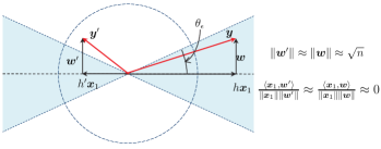
This geometric argument suggests the use of a threshold decoder that, for a given received signal $\bm{Y}$, declares $\bm{x}_{i}$ to be the transmitted codeword if $\bm{x}_{i}$ is the only codeword for which $\theta(\bm{x}_{i},\bm{Y})\leq\theta_{\epsilon}$. If no codewords or more than one codeword meet this condition, the decoder declares an error. Thresholding angles instead of log-likelihood ratios (cf., [9, Th. 17 and Th. 25]) appears to be a natural approach when CSIR is unavailable. Note that the proposed threshold decoder does neither require CSIR nor knowledge of the fading distribution. As we shall see, it achieves (4) and yields a tight achievability bound at finite blocklength, provided that the threshold $\theta_{\epsilon}$ is chosen appropriately.

In the following, we generalize the aforementioned threshold decoder to the MIMO case and present our achievability results.

IV-A2 The Achievability Bound

To state our achievability (lower) bound on $R_{\mathrm{tx}}^{\ast}(n,\epsilon)$, we will need the following definition, which extends the notion of angle between real vectors to complex subspaces.

Definition 5

Let $\mathcal{A}$ and $\mathcal{B}$ be subspaces in \use@mathgroup\M@U\symAMSbCn\use@mathgroup\M@U\symAMSbsuperscript𝐶𝑛\use@mathgroup\M@U\symAMSb{C}^{n} with $a=\dim(\mathcal{A})\leq\dim(\mathcal{B})=b$. The principal angles $0\leq\theta_{1}\leq\cdots\leq\theta_{a}\leq{\pi}/{2}$ between $\mathcal{A}$ and $\mathcal{B}$ are defined recursively by

$$\cos\theta_{k}\triangleq\!\!\!\max\limits_{\scriptsize\begin{array}[]{c}\bm{a}\in\mathcal{A},\bm{b}\in\mathcal{B}\colon\|\bm{a}\|=\|\bm{b}\|=1,\\ \langle\bm{a},\bm{a}_{i}\rangle=\langle\bm{b},\bm{b}_{i}\rangle=0,i=1,\ldots,k-1\end{array}}\!\!\!\!|\langle\bm{a},\bm{b}\rangle|,\\ \quad k=1,\ldots,a.$$ (39)

Here, $\bm{a}_{k}$ and $\bm{b}_{k}$, $k=1,\ldots,a$, are the vectors that achieve the maximum in (39) at the $k$th recursion. The angle between the subspaces $\mathcal{A}$ and $\mathcal{B}$ is defined by

$\displaystyle\sin\{\mathcal{A},\mathcal{B}\}\triangleq\prod\limits_{k=1}^{a}\sin\theta_{k}.$ (40)

With a slight abuse of notation, for two matrices 𝖠\use@mathgroup\M@U\symAMSbCn×a𝖠\use@mathgroup\M@U\symAMSbsuperscript𝐶𝑛𝑎\mathsf{A}\in\use@mathgroup\M@U\symAMSb{C}^{n\times a} and 𝖡\use@mathgroup\M@U\symAMSbCn×b𝖡\use@mathgroup\M@U\symAMSbsuperscript𝐶𝑛𝑏\mathsf{B}\in\use@mathgroup\M@U\symAMSb{C}^{n\times b}, we abbreviate $\sin\mathopen{}\left\{\mathrm{span}(\mathsf{A}),\mathrm{span}(\mathsf{B})\right\}$ with $\sin\{\mathsf{A},\mathsf{B}\}$. When the columns of $\mathsf{A}$ and $\mathsf{B}$ are orthonormal bases for $\mathrm{span}(\mathsf{A})$ and $\mathrm{span}(\mathsf{B})$, respectively, we have (see, e.g., [22, Sec. I])

$\displaystyle\sin^{2}\{\mathsf{A},\mathsf{B}\}$ $\displaystyle=$ $\displaystyle\det\mathopen{}\left(\mathsf{I}-\mathsf{A}^{\mathrm{H}}\mathsf{B}\mathsf{B}^{\mathrm{H}}\mathsf{A}\right)$ (41)
$\displaystyle=$ $\displaystyle\det\mathopen{}\left(\mathsf{I}-\mathsf{B}^{\mathrm{H}}\mathsf{A}\mathsf{A}^{\mathrm{H}}\mathsf{B}\right).$ (42)

Some additional properties of the operator $\sin\{\cdot,\cdot\}$ are listed in Appendix A.

We are now ready to state our achievability bound.

Theorem 1

Let $\Lambda_{1}\geq\cdots\geq\Lambda_{m}$ be the $m$ largest eigenvalues of \use@mathgroup\M@U\symAMSbH\use@mathgroup\M@U\symAMSbHH\use@mathgroup\M@U\symAMSb𝐻\use@mathgroup\M@U\symAMSbsuperscript𝐻H\use@mathgroup\M@U\symAMSb{H}\use@mathgroup\M@U\symAMSb{H}^{\mathrm{H}}. For every $0\!<\!\epsilon\!<\!1$ and every $0\!<\!\tau\!<\!\epsilon$, there exists an $(n,M,\epsilon)_{\mathrm{tx}}$ code for the channel (8) that satisfies

$\displaystyle\frac{\log M}{n}$ $\displaystyle\geq$ 1nlogτ\use@mathgroup\M@U\symAMSbP[j=1rBjγn].1𝑛𝜏\use@mathgroup\M@U\symAMSb𝑃delimited-[]superscriptsubscriptproduct𝑗1𝑟subscript𝐵𝑗subscript𝛾𝑛\displaystyle\frac{1}{n}\log\frac{\tau}{\use@mathgroup\M@U\symAMSb{P}\mathopen{}\big{[}\prod_{j=1}^{r}B_{j}\leq\gamma_{n}\big{]}}. (43)

Here, $B_{j}\sim\mathrm{Beta}(n-t-j+1,t)$, $j=1,\ldots,r$, are independent Beta-distributed random variables, and $\gamma_{n}\in[0,1]$ is chosen so that

\IEEEeqnarraymulticol3l\use@mathgroup\M@U\symAMSbP[sin2{𝖨n,t,n𝖨n,tdiag{v1Λ1,,\displaystyle\IEEEeqnarraymulticol{3}{l}{\use@mathgroup\M@U\symAMSb{P}\mathopen{}\bigg{[}\sin^{2}\mathopen{}\Big{\{}\mathsf{I}_{n,t},\sqrt{n}\mathsf{I}_{n,t}\mathrm{diag}\mathopen{}\Big{\{}\sqrt{v_{1}^{*}\Lambda_{1}},\ldots,}
vmΛm,0,,0tm}+\use@mathgroup\M@U\symAMSbW}γn]1ϵ+τ\displaystyle\quad\quad\quad\sqrt{v_{m}^{*}\Lambda_{m}},\underbrace{0,\ldots,0}_{t-m}\Big{\}}+\use@mathgroup\M@U\symAMSb{W}\Big{\}}\leq\gamma_{n}\bigg{]}\geq 1-\epsilon+\tau (44)

where

$\displaystyle v^{\ast}_{j}=[\bar{\gamma}-1/\Lambda_{j}]^{+},\,\,\,j=1,\ldots,r$ (45)

are the water-filling power gains and $\bar{\gamma}$ is defined in (22).

Proof:

The achievability bound is based on a decoder that operates as follows: it first computes the sine of the angle between the subspace spanned by the received matrix \use@mathgroup\M@U\symAMSbY\use@mathgroup\M@U\symAMSb𝑌\use@mathgroup\M@U\symAMSb{Y} and the subspace spanned by each codeword; then, it chooses the first codeword for which the squared sine of the angle is below $\gamma_{n}$. To analyze the performance of this decoder, we apply the $\kappa\beta$ bound [9, Th. 25] to a physically degraded channel whose output is span(\use@mathgroup\M@U\symAMSbY)span\use@mathgroup\M@U\symAMSb𝑌\mathrm{span}(\use@mathgroup\M@U\symAMSb{Y}). See Appendix B for the complete proof. ∎

IV-B Converse

In this section, we shall assume both CSIR and CSIT. Our converse bound is based on the meta-converse theorem [9, Th. 30]. Since CSI is available at both the transmitter and the receiver, the MIMO channel (8) can be transformed into a set of parallel quasi-static channels. The proof of Theorem 2 below builds on [23, Sec. 4.5], which characterizes the nonasymptotic coding rate of parallel AWGN channels.

Theorem 2

Let $\Lambda_{1}\geq\cdots\geq\Lambda_{m}$ be the $m$ largest eigenvalues of \use@mathgroup\M@U\symAMSbH\use@mathgroup\M@U\symAMSbHH\use@mathgroup\M@U\symAMSb𝐻\use@mathgroup\M@U\symAMSbsuperscript𝐻H\use@mathgroup\M@U\symAMSb{H}\use@mathgroup\M@U\symAMSb{H}^{\mathrm{H}}, and let $\bm{\Lambda}\triangleq[\Lambda_{1},\ldots,\Lambda_{m}]^{\mathrm{T}}$. Consider an arbitrary power-allocation function 𝐯:\use@mathgroup\M@U\symAMSbR+m𝒱m:𝐯maps-to\use@mathgroup\M@U\symAMSbsuperscriptsubscript𝑅𝑚subscript𝒱𝑚\bm{v}:\use@mathgroup\M@U\symAMSb{R}_{+}^{m}\mapsto\mathcal{V}_{m}, where

𝒱m{[p1,,pm]\use@mathgroup\M@U\symAMSbR+m:j=1mpjρ}.subscript𝒱𝑚conditional-setsubscript𝑝1subscript𝑝𝑚\use@mathgroup\M@U\symAMSbsuperscriptsubscript𝑅𝑚superscriptsubscript𝑗1𝑚subscript𝑝𝑗𝜌\displaystyle\mathcal{V}_{m}\triangleq\left\{[p_{1},\ldots,p_{m}]\in\use@mathgroup\M@U\symAMSb{R}_{+}^{m}:\,\sum\nolimits_{j=1}^{m}p_{j}\leq\rho\right\}. (46)

Let

$\displaystyle L^{\mathrm{rt}}_{n}(\bm{v},\bm{\Lambda})$ $\displaystyle\triangleq$ $\displaystyle\sum\limits_{i=1}^{n}\sum\limits_{j=1}^{m}\!\Bigg{(}\!\log\mathopen{}\big{(}1+\Lambda_{j}v_{j}(\bm{\Lambda})\big{)}+1$ (47)
$\displaystyle-\,\left|\sqrt{\Lambda_{j}v_{j}(\bm{\Lambda})}Z_{i,j}-\sqrt{1+\Lambda_{j}v_{j}(\bm{\Lambda})}\right|^{2}\!\Bigg{)}$

and

$\displaystyle S^{\mathrm{rt}}_{n}(\bm{v},\bm{\Lambda})$ $\displaystyle\triangleq$ $\displaystyle\sum\limits_{i=1}^{n}\sum\limits_{j=1}^{m}\Bigg{(}\!\log\mathopen{}\big{(}1+\Lambda_{j}v_{j}(\bm{\Lambda})\big{)}+1$ (48)
$\displaystyle\quad\quad\quad\quad\,\,-\,\frac{\big{|}\sqrt{\Lambda_{j}v_{j}(\bm{\Lambda})}Z_{ij}-1\big{|}^{2}}{1+\Lambda_{j}v_{j}(\bm{\Lambda})}\!\Bigg{)}$

where $v_{j}(\cdot)$ is the $j$th coordinate of $\bm{v}(\cdot)$, and $Z_{ij}$, $i=1,\ldots,n$, $j=1,\ldots,m$, are i.i.d. $\mathcal{CN}(0,1)$ distributed random variables. For every $n$ and every $0<\epsilon<1$, the maximal achievable rate on the channel (8) with CSIRT is upper-bounded by

Rrt(n,ϵ)1nlogcrt(n)inf𝒗()\use@mathgroup\M@U\symAMSbP[Lnrt(𝒗,𝚲)nγn(𝒗)]superscriptsubscript𝑅rt𝑛italic-ϵ1𝑛subscript𝑐rt𝑛subscriptinfimum𝒗\use@mathgroup\M@U\symAMSb𝑃delimited-[]subscriptsuperscript𝐿rt𝑛𝒗𝚲𝑛subscript𝛾𝑛𝒗\displaystyle R_{\mathrm{rt}}^{\ast}(n,\epsilon)\leq\frac{1}{n}\log\frac{c_{\mathrm{rt}}(n)}{\inf\limits_{\bm{v}(\cdot)}\use@mathgroup\M@U\symAMSb{P}[L^{\mathrm{rt}}_{n}(\bm{v},\bm{\Lambda})\geq n\gamma_{n}(\bm{v})]} (49)

where

$\displaystyle c_{\mathrm{rt}}(n)$ $\displaystyle\triangleq$ $\displaystyle\left(\frac{(n-1)^{n}e^{-(n-1)}}{\Gamma(n)}+\frac{\Gamma(n,n-1)}{\Gamma(n)}\right)^{m}$ (50)
×\use@mathgroup\M@U\symAMSbE\use@mathgroup\M@U\symAMSbH[det(𝖨t+ρ\use@mathgroup\M@U\symAMSbH\use@mathgroup\M@U\symAMSbHH)]absent\use@mathgroup\M@U\symAMSbsubscript𝐸\use@mathgroup\M@U\symAMSb𝐻delimited-[]subscript𝖨𝑡𝜌\use@mathgroup\M@U\symAMSb𝐻\use@mathgroup\M@U\symAMSbsuperscript𝐻H\displaystyle\times\,\use@mathgroup\M@U\symAMSb{E}_{\use@mathgroup\M@U\symAMSb{H}}\mathopen{}\left[\det(\mathsf{I}_{t}+\rho\use@mathgroup\M@U\symAMSb{H}\use@mathgroup\M@U\symAMSb{H}^{\mathrm{H}})\right]

and the scalar $\gamma_{n}(\bm{v})$ is the solution of

\use@mathgroup\M@U\symAMSbP[Snrt(𝒗,𝚲)nγn(𝒗)]=ϵ.\use@mathgroup\M@U\symAMSb𝑃delimited-[]subscriptsuperscript𝑆rt𝑛𝒗𝚲𝑛subscript𝛾𝑛𝒗italic-ϵ\displaystyle\use@mathgroup\M@U\symAMSb{P}[S^{\mathrm{rt}}_{n}(\bm{v},\bm{\Lambda})\leq n\gamma_{n}(\bm{v})]=\epsilon. (51)

The infimum on the RHS of (49) is taken over all power allocation functions 𝐯:\use@mathgroup\M@U\symAMSbR+m𝒱m:𝐯maps-to\use@mathgroup\M@U\symAMSbsuperscriptsubscript𝑅𝑚subscript𝒱𝑚\bm{v}:\use@mathgroup\M@U\symAMSb{R}_{+}^{m}\mapsto\mathcal{V}_{m}.

Proof:

See Appendix C. ∎

Remark 1

The infimum on the RHS of (49) makes the converse bound in Theorem 2 difficult to evaluate numerically. We can further upper-bound the RHS of (49) by lower-bounding \use@mathgroup\M@U\symAMSbP[Lnrt(𝐯,𝚲)nγn(𝐯)]\use@mathgroup\M@U\symAMSb𝑃delimited-[]subscriptsuperscript𝐿rt𝑛𝐯𝚲𝑛subscript𝛾𝑛𝐯\use@mathgroup\M@U\symAMSb{P}[L^{\mathrm{rt}}_{n}(\bm{v},\bm{\Lambda})\geq n\gamma_{n}(\bm{v})] for each $\bm{v}(\cdot)$ using [9, Eq. (102)] and the Chernoff bound. After doing so, the infimum can be computed analytically and the resulting upper bound on $R_{\mathrm{rt}}^{\ast}(n,\epsilon)$ allows for numerical evaluations. Unfortunately, this bound is in general loose.

Remark 2

As we shall discuss in Section V-B, the bound (49) can be tightened and evaluated numerically in the SIMO case or when the codewords are isotropic, i.e., are chosen from the set $\mathcal{F}_{\mathrm{iso}}$ in (32). Note that in both scenarios CSIT is not beneficial.

IV-C Asymptotic Analysis

Following [9, Def. 2], we define the $\epsilon$-dispersion of the channel (8) with CSIT via $R_{\mathrm{tx}}^{\ast}(n,\epsilon)$ (resp. $R_{\mathrm{rt}}^{\ast}(n,\epsilon)$) as

$$V_{\epsilon}^{l}\triangleq\limsup\limits_{n\to\infty}n\left(\frac{C_{\epsilon}^{\mathrm{tx}}-R^{\ast}_{l}(n,\epsilon)}{Q^{-1}(\epsilon)}\right)^{2},\\ \,\,\epsilon\in(0,1)\backslash\{1/2\},\,l=\{\mathrm{tx},\mathrm{rt}\}.$$ (52)

Theorem 3 below characterizes the $\epsilon$-dispersion of the quasi-static fading channel (8) with CSIT.

Theorem 3

Assume that the fading channel \use@mathgroup\M@U\symAMSbH\use@mathgroup\M@U\symAMSb𝐻\use@mathgroup\M@U\symAMSb{H} satisfies the following conditions:

  1. 1.

    the expectation \use@mathgroup\M@U\symAMSbE\use@mathgroup\M@U\symAMSbH[det(𝖨t+ρ\use@mathgroup\M@U\symAMSbH\use@mathgroup\M@U\symAMSbHH)]\use@mathgroup\M@U\symAMSbsubscript𝐸\use@mathgroup\M@U\symAMSb𝐻delimited-[]subscript𝖨𝑡𝜌\use@mathgroup\M@U\symAMSb𝐻\use@mathgroup\M@U\symAMSbsuperscript𝐻H\use@mathgroup\M@U\symAMSb{E}_{\use@mathgroup\M@U\symAMSb{H}}\mathopen{}\left[\det(\mathsf{I}_{t}+\rho\use@mathgroup\M@U\symAMSb{H}\use@mathgroup\M@U\symAMSb{H}^{\mathrm{H}})\right] is finite;

  2. 2.

    the joint pdf of the ordered nonzero eigenvalues of \use@mathgroup\M@U\symAMSbHH\use@mathgroup\M@U\symAMSbH\use@mathgroup\M@U\symAMSbsuperscript𝐻H\use@mathgroup\M@U\symAMSb𝐻\use@mathgroup\M@U\symAMSb{H}^{\mathrm{H}}\use@mathgroup\M@U\symAMSb{H} exists and is continuously differentiable;

  3. 3.

    $C_{\epsilon}^{\mathrm{tx}}$ is a point of growth of the outage probability function (20) , i.e.,666Note that this condition implies that $C_{\epsilon}^{\mathrm{tx}}$ is a continuous function of $\epsilon$ (see Section III).

    $\displaystyle F_{\mathrm{tx}}^{\prime}\mathopen{}\left(C_{\epsilon}^{\mathrm{tx}}\right)>0.$ (53)

Then

$\displaystyle\big{\{}R_{\mathrm{tx}}^{\ast}(n,\epsilon),R_{\mathrm{rt}}^{\ast}(n,\epsilon)\big{\}}$ $\displaystyle=$ $\displaystyle C_{\epsilon}^{\mathrm{tx}}+\mathcal{O}\mathopen{}\left(\frac{\log n}{n}\right).$ (54)

Hence, the $\epsilon$-dispersion is zero for both the CSIRT and the CSIT case:

$\displaystyle V_{\epsilon}^{\mathrm{tx}}=V_{\epsilon}^{\mathrm{rt}}=0,\quad\,\,\epsilon\in(0,1)\backslash\{1/2\}.$ (55)
Proof:

To prove (54), we first establish in Appendix D the converse result

$\displaystyle R_{\mathrm{rt}}^{\ast}(n,\epsilon)\leq C_{\epsilon}^{\mathrm{tx}}+\mathcal{O}\mathopen{}\left(\frac{\log n}{n}\right)$ (56)

by analyzing the upper bound (49) in the limit $n\to\infty$. We next prove in Appendix E the achievability result

$\displaystyle R_{\mathrm{tx}}^{\ast}(n,\epsilon)\geq C_{\epsilon}^{\mathrm{tx}}+\mathcal{O}\mathopen{}\left(\frac{\log n}{n}\right)$ (57)

by expanding (43) for $n\to\infty$. The desired result then follows by (14). ∎

Remark 3

As mentioned in Section I, the quasi-static fading channel considered in this paper belongs to the general class of composite or mixed channels, whose $\epsilon$-dispersion is known in some special cases. Specifically, the dispersion of a mixed channel with two states was derived in [24, Th. 7]. This result was extended to channels with finitely many states in [25, Th. 4]. In both cases, the rate of convergence to the $\epsilon$-capacity is $\mathcal{O}(1/\sqrt{n})$ (positive dispersion), as opposed to $\mathcal{O}(\log(n)/n)$ in Theorem 3. Our result shows that moving from finitely many to uncountably many states (as in the quasi-static fading case) yields a drastic change in the value of the channel dispersion. For this reason, our result is not derivable from [24] or [25].

Remark 4

It can be shown that the assumptions on the fading matrix in Theorem 3 are satisfied by most probability distributions used to model MIMO fading channels, such as i.i.d. or correlated Rayleigh, Rician, and Nakagami. However, the (nonfading) AWGN MIMO channel, which can be seen as a quasi-static fading channel with fading distribution equal to a step function, does not meet these assumptions and has, in fact, positive dispersion [23, Th. 78].

While zero dispersion indeed may imply fast convergence to $\epsilon$-capacity, this is not true anymore when the probability distribution of the fading matrix approaches a step function, in which case the higher-order terms in the expansion (54) become more dominant. Consider for example a SISO Rician fading channel with Rician factor $K$. For $\epsilon<1/2$, one can refine (54) and show that [26]

$\displaystyle C_{\epsilon}-\frac{\log n}{n}-\frac{c_{1}\sqrt{K}+c_{2}}{n}+\mathit{o}\mathopen{}\left(\frac{1}{n}\right)\leq R_{\mathrm{tx}}^{\ast}(n,\epsilon)$
$\displaystyle\quad\quad\leq R_{\mathrm{rt}}^{\ast}(n,\epsilon)\leq C_{\epsilon}+\frac{\log n}{n}-\frac{\tilde{c}_{1}\sqrt{K}+\tilde{c}_{2}}{n}+\mathit{o}\mathopen{}\left(\frac{1}{n}\right)$ (58)

where $c_{1}$, $c_{2}$, $\tilde{c}_{1}$ and $\tilde{c}_{2}$ are finite constants with $c_{1}>0$ and $\tilde{c}_{1}>0$. As we let the Rician factor $K$ become large, the fading distribution converges to a step function and the third term in both the left-most lower bound and the right-most upper bound becomes increasingly large in absolute value.

IV-D Normal Approximation

We define the normal approximation $R_{\mathrm{rt}}^{\mathcal{N}}(n,\epsilon)$ of $R_{\mathrm{rt}}^{*}(n,\epsilon)$ as the solution of

$\displaystyle\epsilon$ $\displaystyle=$ \use@mathgroup\M@U\symAMSbE[Q(C(\use@mathgroup\M@U\symAMSbH)Rrt𝒩(n,ϵ)V(\use@mathgroup\M@U\symAMSbH)/n)].\use@mathgroup\M@U\symAMSb𝐸delimited-[]𝑄𝐶\use@mathgroup\M@U\symAMSb𝐻superscriptsubscript𝑅rt𝒩𝑛italic-ϵ𝑉\use@mathgroup\M@U\symAMSb𝐻𝑛\displaystyle\use@mathgroup\M@U\symAMSb{E}\mathopen{}\left[Q\mathopen{}\left(\frac{C(\use@mathgroup\M@U\symAMSb{H})-R_{\mathrm{rt}}^{\mathcal{N}}(n,\epsilon)}{\sqrt{V(\use@mathgroup\M@U\symAMSb{H})/n}}\right)\right]. (59)

Here,

$\displaystyle C(\mathsf{H})=\sum\limits_{j=1}^{m}\log(1+v_{j}^{\ast}\lambda_{j})$ (60)

is the capacity of the channel (8) when \use@mathgroup\M@U\symAMSbH=𝖧\use@mathgroup\M@U\symAMSb𝐻𝖧\use@mathgroup\M@U\symAMSb{H}=\mathsf{H} (the water-filling power allocation values $\{v_{j}^{\ast}\}$ in (60) are given in (45) and $\{\lambda_{j}\}$ are the eigenvalues of $\mathsf{H}^{\mathrm{H}}\mathsf{H}$), and

$\displaystyle V(\mathsf{H})=m-\sum\limits_{j=1}^{m}\frac{1}{(1+v_{j}^{\ast}\lambda_{j})^{2}}$ (61)

is the dispersion of the channel (8) when \use@mathgroup\M@U\symAMSbH=𝖧\use@mathgroup\M@U\symAMSb𝐻𝖧\use@mathgroup\M@U\symAMSb{H}=\mathsf{H} [23, Th. 78]. Theorem 3 and the expansion

$\displaystyle R_{\mathrm{rt}}^{\mathcal{N}}(n,\epsilon)=C_{\epsilon}^{\mathrm{tx}}+\mathcal{O}\mathopen{}\left(\frac{1}{n}\right)$ (62)

(which follows from Lemma 17 in Appendix D-C and Taylor’s theorem) suggest that this approximation is accurate, as confirmed by the numerical results reported in Section VI-A. Note that the same approximation has been concurrently proposed in [27]; see also [24, Def. 2] and [25, Sec. 4] for similar approximations for mixed channels with finitely many states.

V CSI Not Available at the Transmitter

V-A Achievability

In this section, we shall assume that neither the transmitter nor the receiver have a priori CSI. Using the decoder described in IV-A, we obtain the following achievability bound.

Theorem 4

Assume that for a given $0<\epsilon<1$ there exists a $\mathsf{Q}^{\ast}\in\mathcal{U}_{t}$ such that

$\displaystyle F_{\mathrm{no}}(C_{\epsilon}^{\mathrm{no}})$ $\displaystyle=$ inf𝖰𝒰t\use@mathgroup\M@U\symAMSbP[logdet(𝖨r+\use@mathgroup\M@U\symAMSbHH𝖰\use@mathgroup\M@U\symAMSbH)Cϵno]subscriptinfimum𝖰subscript𝒰𝑡\use@mathgroup\M@U\symAMSb𝑃delimited-[]subscript𝖨𝑟\use@mathgroup\M@U\symAMSbsuperscript𝐻H𝖰\use@mathgroup\M@U\symAMSb𝐻superscriptsubscript𝐶italic-ϵno\displaystyle\inf_{\mathsf{Q}\in\mathcal{U}_{t}}\use@mathgroup\M@U\symAMSb{P}\mathopen{}\left[\log\det\mathopen{}\left(\mathsf{I}_{r}+\use@mathgroup\M@U\symAMSb{H}^{\mathrm{H}}\mathsf{Q}\use@mathgroup\M@U\symAMSb{H}\right)\leq C_{\epsilon}^{\mathrm{no}}\right] (63)
$\displaystyle=$ \use@mathgroup\M@U\symAMSbP[logdet(𝖨r+\use@mathgroup\M@U\symAMSbHH𝖰\use@mathgroup\M@U\symAMSbH)Cϵno]\use@mathgroup\M@U\symAMSb𝑃delimited-[]subscript𝖨𝑟\use@mathgroup\M@U\symAMSbsuperscript𝐻Hsuperscript𝖰\use@mathgroup\M@U\symAMSb𝐻superscriptsubscript𝐶italic-ϵno\displaystyle\use@mathgroup\M@U\symAMSb{P}\mathopen{}\left[\log\det\mathopen{}\left(\mathsf{I}_{r}+\use@mathgroup\M@U\symAMSb{H}^{\mathrm{H}}\mathsf{Q}^{\ast}\use@mathgroup\M@U\symAMSb{H}\right)\leq C_{\epsilon}^{\mathrm{no}}\right] (64)

i.e., the infimum in (63) is a minimum. Then, for every $0\!<\!\tau\!<\!\epsilon$ there exists an $(n,M,\epsilon)_{\mathrm{no}}$ code for the channel (8) that satisfies

$\displaystyle\frac{\log M}{n}$ $\displaystyle\geq$ 1nlogτ\use@mathgroup\M@U\symAMSbP[j=1rBjγn].1𝑛𝜏\use@mathgroup\M@U\symAMSb𝑃delimited-[]superscriptsubscriptproduct𝑗1𝑟subscript𝐵𝑗subscript𝛾𝑛\displaystyle\frac{1}{n}\log\frac{\tau}{\use@mathgroup\M@U\symAMSb{P}\mathopen{}\big{[}\prod_{j=1}^{r}B_{j}\leq\gamma_{n}\big{]}}\,. (65)

Here, $B_{j}\sim\mathrm{Beta}(n-t^{\ast}-j+1,t^{\ast})$, $j=1,\ldots,r$, are independent Beta-distributed random variables, $t^{\ast}\triangleq\mathrm{rank}(\mathsf{Q}^{\ast})$, and $\gamma_{n}\in[0,1]$ is chosen so that

\use@mathgroup\M@U\symAMSbP[sin2{𝖨n,t,n𝖨n,t𝖴\use@mathgroup\M@U\symAMSbH+\use@mathgroup\M@U\symAMSbW}γn]1ϵ+τ\use@mathgroup\M@U\symAMSb𝑃delimited-[]superscript2subscript𝖨𝑛superscript𝑡𝑛subscript𝖨𝑛superscript𝑡𝖴\use@mathgroup\M@U\symAMSb𝐻\use@mathgroup\M@U\symAMSb𝑊subscript𝛾𝑛1italic-ϵ𝜏\displaystyle\use@mathgroup\M@U\symAMSb{P}\mathopen{}\left[\sin^{2}\{\mathsf{I}_{n,t^{\ast}},\sqrt{n}\mathsf{I}_{n,t^{\ast}}\mathsf{U}\use@mathgroup\M@U\symAMSb{H}+\use@mathgroup\M@U\symAMSb{W}\}\leq\gamma_{n}\right]\geq 1-\epsilon+\tau (66)

with 𝖴\use@mathgroup\M@U\symAMSbCt×t𝖴\use@mathgroup\M@U\symAMSbsuperscript𝐶superscript𝑡𝑡\mathsf{U}\in\use@mathgroup\M@U\symAMSb{C}^{t^{\ast}\times t} satisfying $\mathsf{U}^{\mathrm{H}}\mathsf{U}=\mathsf{Q}^{\ast}$.

Proof:

The proof is identical to the proof of Theorem 1, with the only difference that the precoding matrix 𝖯(\use@mathgroup\M@U\symAMSbH)𝖯\use@mathgroup\M@U\symAMSb𝐻\mathsf{P}(\use@mathgroup\M@U\symAMSb{H}) (defined in (108)) is replaced by $\sqrt{n}\mathsf{I}_{n,t^{\ast}}\mathsf{U}$. ∎

The assumption in (64) that the $\epsilon$-capacity-achieving input covariance matrix of the channel (8) exists is mild. A sufficient condition for the existence of $\mathsf{Q}^{\ast}$ is given in the following proposition.

Proposition 5

Assume that \use@mathgroup\M@U\symAMSbE[\use@mathgroup\M@U\symAMSbH𝖥2]<\use@mathgroup\M@U\symAMSb𝐸delimited-[]superscriptsubscriptnorm\use@mathgroup\M@U\symAMSb𝐻𝖥2\use@mathgroup\M@U\symAMSb{E}\mathopen{}\left[\left\|\use@mathgroup\M@U\symAMSb{H}\right\|_{\mathsf{F}}^{2}\right]<\infty and that the distribution of \use@mathgroup\M@U\symAMSbH\use@mathgroup\M@U\symAMSb𝐻\use@mathgroup\M@U\symAMSb{H} is absolutely continuous with respect to the Lebesgue measure on \use@mathgroup\M@U\symAMSbCt×r\use@mathgroup\M@U\symAMSbsuperscript𝐶𝑡𝑟\use@mathgroup\M@U\symAMSb{C}^{t\times r}. Then, for every R\use@mathgroup\M@U\symAMSbR+𝑅\use@mathgroup\M@U\symAMSbsubscript𝑅R\in\use@mathgroup\M@U\symAMSb{R}_{+}, the infimum in (26) is a minimum.

Proof:

See Appendix F. ∎

For the SIMO case, the RHS of (43) and the RHS of (65) coincide, i.e.,

$\displaystyle\big{\{}R_{\mathrm{tx}}(n,\epsilon),R_{\mathrm{no}}(n,\epsilon)\big{\}}$ $\displaystyle\geq$ 1nlogτ\use@mathgroup\M@U\symAMSbP[Bγn]1𝑛𝜏\use@mathgroup\M@U\symAMSb𝑃delimited-[]𝐵subscript𝛾𝑛\displaystyle\frac{1}{n}\log\frac{\tau}{\use@mathgroup\M@U\symAMSb{P}\mathopen{}\left[B\leq\gamma_{n}\right]} (67)

where $B\sim\mathrm{Beta}(n-r,r)$, and $\gamma_{n}\in[0,1]$ is chosen so that

\use@mathgroup\M@U\symAMSbP[sin2{𝒆1,nρ𝒆1𝑯T+\use@mathgroup\M@U\symAMSbW}γn]1ϵ+τ.\use@mathgroup\M@U\symAMSb𝑃delimited-[]superscript2subscript𝒆1𝑛𝜌subscript𝒆1superscript𝑯T\use@mathgroup\M@U\symAMSb𝑊subscript𝛾𝑛1italic-ϵ𝜏\displaystyle\use@mathgroup\M@U\symAMSb{P}[\sin^{2}\{\bm{e}_{1},\sqrt{n\rho}\bm{e}_{1}\bm{H}^{\mathrm{T}}+\use@mathgroup\M@U\symAMSb{W}\}\leq\gamma_{n}]\geq 1-\epsilon+\tau. (68)

Here, $\bm{e}_{1}$ stands for the first column of the identity matrix $\mathsf{I}_{n}$. The achievability bound (67) follows from (43) and (65) by noting that the random variable $B$ on the RHS of (67) has the same distribution as $\prod\nolimits_{i=1}^{r}B_{i}$, where $B_{i}\sim\mathrm{Beta}(n-i,1)$, $i=1,\ldots,r$.

V-B Converse

For the converse, we shall assume CSIR but not CSIT. The counterpart of Theorem 2 is the following result.

Theorem 6

Let $\mathcal{U}_{t}^{\mathrm{e}}$ be as in (28). For an arbitrary $\mathsf{Q}\in\mathcal{U}_{t}^{\mathrm{e}}$, let $\Lambda_{1}\geq\cdots\geq\Lambda_{m}$ be the ordered eigenvalues of \use@mathgroup\M@U\symAMSbHH𝖰\use@mathgroup\M@U\symAMSbH\use@mathgroup\M@U\symAMSbsuperscript𝐻H𝖰\use@mathgroup\M@U\symAMSb𝐻\use@mathgroup\M@U\symAMSb{H}^{\mathrm{H}}\mathsf{Q}\use@mathgroup\M@U\symAMSb{H}. Let

$$L^{\mathrm{rx}}_{n}(\mathsf{Q})\triangleq\sum\limits_{i=1}^{n}\sum\limits_{j=1}^{m}\!\bigg{(}\!\log(1+\Lambda_{j})+1-\bigl{|}\sqrt{\Lambda_{j}}Z_{ij}-\sqrt{1+\Lambda_{j}}\bigr{|}^{2}\bigg{)}$$ (69)

and

$\displaystyle S^{\mathrm{rx}}_{n}(\mathsf{Q})\triangleq\sum\limits_{i=1}^{n}\sum\limits_{j=1}^{m}\bigg{(}\!\log(1+\Lambda_{j})+1-\frac{\big{|}\sqrt{\Lambda_{j}}Z_{ij}-1\big{|}^{2}}{1+\Lambda_{j}}\bigg{)}$ (70)

where $Z_{ij}$, $i=1,\ldots,n$, $j=1,\ldots,m$, are i.i.d. $\mathcal{CN}(0,1)$ distributed. Then, for every $n\geq r$ and every $0<\epsilon<1$, the maximal achievable rate on the quasi-static MIMO fading channel (8) with CSIR is upper-bounded by

Rrx(n1,ϵ)1n1logcrx(n)inf𝖰𝒰te\use@mathgroup\M@U\symAMSbP[Lnrx(𝖰)nγn(𝖰)].superscriptsubscript𝑅rx𝑛1italic-ϵ1𝑛1subscript𝑐rx𝑛subscriptinfimum𝖰superscriptsubscript𝒰𝑡e\use@mathgroup\M@U\symAMSb𝑃delimited-[]subscriptsuperscript𝐿rx𝑛𝖰𝑛subscript𝛾𝑛𝖰\displaystyle R_{\mathrm{rx}}^{\ast}(n-1,\epsilon)\leq\frac{1}{n-1}\log\frac{c_{\mathrm{rx}}(n)}{\inf\limits_{\mathsf{Q}\in\mathcal{U}_{t}^{\mathrm{e}}}\use@mathgroup\M@U\symAMSb{P}[L^{\mathrm{rx}}_{n}(\mathsf{Q})\geq n\gamma_{n}(\mathsf{Q})]}\,. (71)

Here,

$\displaystyle c_{\mathrm{rx}}(n)$ $\displaystyle\triangleq$ πr(r1)Γr(n)Γr(r)\use@mathgroup\M@U\symAMSbE[(1+ρ\use@mathgroup\M@U\symAMSbH𝖥2)(r+1)2/4]superscript𝜋𝑟𝑟1subscriptΓ𝑟𝑛subscriptΓ𝑟𝑟\use@mathgroup\M@U\symAMSb𝐸delimited-[]superscript1𝜌superscriptsubscriptnorm\use@mathgroup\M@U\symAMSb𝐻𝖥2superscript𝑟124\displaystyle\frac{\pi^{r(r-1)}}{\Gamma_{r}(n)\Gamma_{r}(r)}\use@mathgroup\M@U\symAMSb{E}\mathopen{}\left[\left(1+\rho\left\|\use@mathgroup\M@U\symAMSb{H}\right\|_{\mathsf{F}}^{2}\right)^{\lfloor(r+1)^{2}/4\rfloor}\right] (72)
$\displaystyle\times\,\prod\limits_{i=1}^{r}\bigg{[}\left(n+r-2i\right)^{n+r-2i+1}e^{-(n+r-2i)}$
$\displaystyle\quad\quad\quad\,\,+\,\Gamma(n+r-2i+1,n+r-2i)\bigg{]}$

with $\Gamma_{(\cdot)}(\cdot)$ denoting the complex multivariate Gamma function [28, Eq. (83)], and $\gamma_{n}(\mathsf{Q})$ is the solution of

\use@mathgroup\M@U\symAMSbP[Snrx(𝖰)nγn(𝖰)]=ϵ.\use@mathgroup\M@U\symAMSb𝑃delimited-[]subscriptsuperscript𝑆rx𝑛𝖰𝑛subscript𝛾𝑛𝖰italic-ϵ\displaystyle\use@mathgroup\M@U\symAMSb{P}[S^{\mathrm{rx}}_{n}(\mathsf{Q})\leq n\gamma_{n}(\mathsf{Q})]=\epsilon. (73)
Proof:

See Appendix G. ∎

The infimum in (71) makes the upper bound more difficult to evaluate numerically and to analyze asymptotically up to $\mathcal{O}(\log(n)/n)$ terms than the upper bound (49) that we established for the CSIT case. In fact, even the simpler problem of finding the matrix $\mathsf{Q}$ that minimizes limn\use@mathgroup\M@U\symAMSbP[Lnrx(𝖰)nγn]subscript𝑛\use@mathgroup\M@U\symAMSb𝑃delimited-[]subscriptsuperscript𝐿rx𝑛𝖰𝑛subscript𝛾𝑛\lim\limits_{n\to\infty}\use@mathgroup\M@U\symAMSb{P}[L^{\mathrm{rx}}_{n}(\mathsf{Q})\geq n\gamma_{n}] is open. Next, we consider two special cases for which the bound (71) can be tightened and evaluated numerically: the SIMO case and the case where all codewords are chosen from the set $\mathcal{F}_{\mathrm{iso}}$.

V-B1 SIMO case

For the SIMO case, CSIT is not beneficial [26] and the bounds (49) and (71) can be tightened as follows.

Theorem 7

Let

$\displaystyle L_{n}$ $\displaystyle\triangleq$ $\displaystyle n\log(1+\rho G)+\sum\limits_{i=1}^{n}\left(1-\bigl{|}\sqrt{\rho G}Z_{i}-\sqrt{1+\rho G}\bigr{|}^{2}\!\right)$

and

$\displaystyle S_{n}$ $\displaystyle\triangleq$ $\displaystyle n\log(1+\rho G)+\sum\limits_{i=1}^{n}\left(1-\frac{\big{|}\sqrt{\rho G}Z_{i}-1\big{|}^{2}}{1+\rho G}\right)$ (75)

with $G\triangleq\|\bm{H}\|^{2}$ and $Z_{i}$, $i=1,\ldots,n$, i.i.d. $\mathcal{CN}(0,1)$ distributed. For every $n$ and every $0<\epsilon<1$, the maximal achievable rate on the quasi-static fading channel (8) with one transmit antenna and with CSIR (with or without CSIT) is upper-bounded by

Rrx(n1,ϵ)Rrt(n1,ϵ)1n1log1\use@mathgroup\M@U\symAMSbP[Lnnγn]superscriptsubscript𝑅rx𝑛1italic-ϵsuperscriptsubscript𝑅rt𝑛1italic-ϵ1𝑛11\use@mathgroup\M@U\symAMSb𝑃delimited-[]subscript𝐿𝑛𝑛subscript𝛾𝑛\displaystyle R_{\mathrm{rx}}^{\ast}(n-1,\epsilon)\leq R_{\mathrm{rt}}^{\ast}(n-1,\epsilon)\leq\frac{1}{n-1}\log\frac{1}{\use@mathgroup\M@U\symAMSb{P}[L_{n}\geq n\gamma_{n}]} (76)

where $\gamma_{n}$ is the solution of

\use@mathgroup\M@U\symAMSbP[Snnγn]=ϵ.\use@mathgroup\M@U\symAMSb𝑃delimited-[]subscript𝑆𝑛𝑛subscript𝛾𝑛italic-ϵ\displaystyle\use@mathgroup\M@U\symAMSb{P}[S_{n}\leq n\gamma_{n}]=\epsilon. (77)
Proof:

See [26, Th. 1]. The main difference between the proof of Theorem 7 and the proof of Theorem 2 and Theorem 6 is that the simple bound $\epsilon^{\prime}\geq 1-1/M$ on the maximal error probability of the auxiliary channel in the meta-converse theorem [9, Th. 30] suffices to establish the desired result. The more sophisticated bounds reported in Lemma 14 (Appendix C) and Lemma 19 (Appendix G) are not needed. ∎

V-B2 Converse for $(n,M,\epsilon)_{\mathrm{iso}}$ codes

In Theorem 8 below, we establish a converse bound on the maximal achievable rate of $(n,M,\epsilon)_{\mathrm{iso}}$ codes introduced in Section III. As such codes consist of isotropic codewords chosen from the set $\mathcal{F}_{\mathrm{iso}}$ in (32), CSIT is not beneficial also in this scenario.

Theorem 8

Let $L^{\mathrm{rx}}_{n}(\cdot)$ and $S^{\mathrm{rx}}_{n}(\cdot)$ be as in (69) and (70), respectively. Then, for every $n$ and every $0<\epsilon<1$, the maximal achievable rate $R_{\mathrm{rx},\mathrm{iso}}^{\ast}(n,\epsilon)$ of $(n,M,\epsilon)_{\mathrm{iso}}$ codes over the quasi-static MIMO fading channel (8) with CSIR is upper-bounded by

Rrx,iso(n,ϵ)Rrt,iso(n,ϵ)1nlog1\use@mathgroup\M@U\symAMSbP[Lnrx((ρ/t)𝖨t)nγn]superscriptsubscript𝑅rxiso𝑛italic-ϵsuperscriptsubscript𝑅rtiso𝑛italic-ϵ1𝑛1\use@mathgroup\M@U\symAMSb𝑃delimited-[]subscriptsuperscript𝐿rx𝑛𝜌𝑡subscript𝖨𝑡𝑛subscript𝛾𝑛\displaystyle R_{\mathrm{rx},\mathrm{iso}}^{\ast}(n,\epsilon)\leq R_{\mathrm{rt},\mathrm{iso}}^{\ast}(n,\epsilon)\leq\frac{1}{n}\log\frac{1}{\use@mathgroup\M@U\symAMSb{P}[L^{\mathrm{rx}}_{n}((\rho/t)\mathsf{I}_{t})\geq n\gamma_{n}]}
(78)

where $\gamma_{n}$ is the solution of

\use@mathgroup\M@U\symAMSbP[Snrx((ρ/t)𝖨t)nγn]=ϵ.\use@mathgroup\M@U\symAMSb𝑃delimited-[]subscriptsuperscript𝑆rx𝑛𝜌𝑡subscript𝖨𝑡𝑛subscript𝛾𝑛italic-ϵ\displaystyle\use@mathgroup\M@U\symAMSb{P}[S^{\mathrm{rx}}_{n}((\rho/t)\mathsf{I}_{t})\leq n\gamma_{n}]=\epsilon. (79)
Proof:

The proof follows closely the proof of Theorem 6. As in the SIMO case, the main difference is that the simple bound $\epsilon^{\prime}\geq 1-1/M$ on the maximal error probability of the auxiliary channel in the meta-converse theorem [9, Th. 30] suffices to establish (79). ∎

V-C Asymptotic Analysis

To state our dispersion result, we will need the following definition of the gradient $\nabla g$ of a differentiable function g:\use@mathgroup\M@U\symAMSbCt×r\use@mathgroup\M@U\symAMSbR:𝑔maps-to\use@mathgroup\M@U\symAMSbsuperscript𝐶𝑡𝑟\use@mathgroup\M@U\symAMSb𝑅g:\use@mathgroup\M@U\symAMSb{C}^{t\times r}\mapsto\use@mathgroup\M@U\symAMSb{R}. Let 𝖫\use@mathgroup\M@U\symAMSbCt×r𝖫\use@mathgroup\M@U\symAMSbsuperscript𝐶𝑡𝑟\mathsf{L}\in\use@mathgroup\M@U\symAMSb{C}^{t\times r}, then we shall write $\nabla g(\mathsf{H})=\mathsf{L}$ if

ddtg(𝖧+t𝖠)|t=0=Re{tr(𝖠H𝖫)},𝖠\use@mathgroup\M@U\symAMSbCt×r.formulae-sequenceevaluated-at𝑑𝑑𝑡𝑔𝖧𝑡𝖠𝑡0Retrsuperscript𝖠H𝖫for-all𝖠\use@mathgroup\M@U\symAMSbsuperscript𝐶𝑡𝑟\displaystyle\frac{d}{dt}g(\mathsf{H}+t\mathsf{A})\Big{|}_{t=0}=\mathrm{Re}\mathopen{}\left\{\mathrm{tr}\mathopen{}\big{(}\mathsf{A}^{\mathrm{H}}\mathsf{L}\big{)}\right\},\quad\forall\mathsf{A}\in\use@mathgroup\M@U\symAMSb{C}^{t\times r}. (80)

Theorem 9 below establishes the zero-dispersion result for the case of no CSIT. Because of the analytical intractability of the minimization in the converse bound (71), Theorem 9 requires more stringent conditions on the fading distribution compared to the CSIT case (cf., Theorem 3), and its proof is more involved.

Theorem 9

Let f\use@mathgroup\M@U\symAMSbHsubscript𝑓\use@mathgroup\M@U\symAMSb𝐻f_{\use@mathgroup\M@U\symAMSb{H}} be the pdf of the fading matrix \use@mathgroup\M@U\symAMSbH\use@mathgroup\M@U\symAMSb𝐻\use@mathgroup\M@U\symAMSb{H}. Assume that \use@mathgroup\M@U\symAMSbH\use@mathgroup\M@U\symAMSb𝐻\use@mathgroup\M@U\symAMSb{H} satisfies the following conditions:

  1. 1.

    f\use@mathgroup\M@U\symAMSbHsubscript𝑓\use@mathgroup\M@U\symAMSb𝐻f_{\use@mathgroup\M@U\symAMSb{H}} is a smooth function, i.e., it has derivatives of all orders.

  2. 2.

    There exists a positive constant $a$ such that

    f\use@mathgroup\M@U\symAMSbH(𝖧)subscript𝑓\use@mathgroup\M@U\symAMSb𝐻𝖧\displaystyle f_{\use@mathgroup\M@U\symAMSb{H}}(\mathsf{H}) $\displaystyle\leq$ $\displaystyle a\left\|\mathsf{H}\right\|_{\mathsf{F}}^{-2tr-\lfloor(r+1)^{2}/2\rfloor-1}$ (81)
    f\use@mathgroup\M@U\symAMSbH(𝖧)𝖥subscriptnormsubscript𝑓\use@mathgroup\M@U\symAMSb𝐻𝖧𝖥\displaystyle\left\|\nabla f_{\use@mathgroup\M@U\symAMSb{H}}(\mathsf{H})\right\|_{\mathsf{F}} $\displaystyle\leq$ $\displaystyle a\left\|\mathsf{H}\right\|_{\mathsf{F}}^{-2tr-5}.$ (82)
  3. 3.

    The function $F_{\mathrm{no}}(\cdot)$ satisfies

    $\displaystyle\liminf\limits_{\delta\to 0}\frac{F_{\mathrm{no}}(C_{\epsilon}^{\mathrm{no}}+\delta)-F_{\mathrm{no}}(C_{\epsilon}^{\mathrm{no}})}{\delta}>0.$ (83)

Then,

$\displaystyle\big{\{}R_{\mathrm{no}}^{\ast}(n,\epsilon),R_{\mathrm{rx}}^{\ast}(n,\epsilon)\big{\}}$ $\displaystyle=$ $\displaystyle C_{\epsilon}^{\mathrm{no}}+\mathcal{O}\mathopen{}\left(\frac{\log n}{n}\right).$ (84)

Hence, the $\epsilon$-dispersion is zero for both the CSIR and the no-CSI case:

$\displaystyle V_{\epsilon}^{\mathrm{no}}=V_{\epsilon}^{\mathrm{rx}}=0,\quad\,\,\epsilon\in(0,1)\backslash\{1/2\}.$ (85)
Proof:

See Appendices H and I. ∎

Remark 5

It can be shown that Conditions 13 in Theorem 9 are satisfied by the probability distributions commonly used to model MIMO fading channels, such as Rayleigh, Rician, and Nakagami. Condition 2 requires simply that f\use@mathgroup\M@U\symAMSbHsubscript𝑓\use@mathgroup\M@U\symAMSb𝐻f_{\use@mathgroup\M@U\symAMSb{H}} has a polynomially decaying tail. Condition 3 plays the same role as (53) in the CSIT case. The exact counterpart of (53) for the no-CSIT case would be

$\displaystyle F_{\mathrm{no}}^{\prime}(C_{\epsilon}^{\mathrm{no}})>0.$ (86)

However, different from (53), the inequality (86) does not necessarily hold for the commonly used fading distributions. Indeed, consider a MISO i.i.d. Rayleigh-fading channel. As proven in [20], the $\epsilon$-capacity-achieving covariance matrix for this case is given by (29). The resulting outage probability function $F_{\mathrm{no}}(\cdot)$ may not be differentiable at the rates $R$ for which the infimum in (27) is achieved by two input covariance matrices with different number of nonzero entries $t^{*}$ on the main diagonal.

Next, we briefly sketch how to prove that Condition 3 holds for Rayleigh, Rician, and Nakagami distributions. Let

F𝖰(R)\use@mathgroup\M@U\symAMSbP[logdet(𝖨r+\use@mathgroup\M@U\symAMSbHH𝖰\use@mathgroup\M@U\symAMSbH)<R].subscript𝐹𝖰𝑅\use@mathgroup\M@U\symAMSb𝑃delimited-[]subscript𝖨𝑟\use@mathgroup\M@U\symAMSbsuperscript𝐻H𝖰\use@mathgroup\M@U\symAMSb𝐻𝑅F_{\mathsf{Q}}(R)\triangleq\use@mathgroup\M@U\symAMSb{P}[\log\det\mathopen{}\left(\mathsf{I}_{r}+\use@mathgroup\M@U\symAMSb{H}^{\mathrm{H}}\mathsf{Q}\use@mathgroup\M@U\symAMSb{H}\right)<R]. (87)

Let $\mathcal{Q}_{\epsilon}$ be the set of all $\epsilon$-capacity-achieving covariance matrices, i.e.,

$\displaystyle\mathcal{Q}_{\epsilon}\triangleq\{\mathsf{Q}\in\mathcal{U}_{t}^{\mathrm{e}}:F_{\mathsf{Q}}(C_{\epsilon}^{\mathrm{no}})=F_{\mathrm{no}}(C_{\epsilon}^{\mathrm{no}})\}.$ (88)

By Proposition 5, the set $\mathcal{Q}_{\epsilon}$ is non-empty for the considered fading distributions. It follows from algebraic manipulations that

$\displaystyle\liminf\limits_{\delta\to 0}\frac{F_{\mathrm{no}}(C_{\epsilon}^{\mathrm{no}}+\delta)-F_{\mathrm{no}}(C_{\epsilon}^{\mathrm{no}})}{\delta}=\inf\limits_{\mathsf{Q}\in\mathcal{Q}_{\epsilon}}F_{\mathsf{Q}}^{\prime}(C_{\epsilon}^{\mathrm{no}}).$ (89)

To show that the RHS of (89) is positive, one needs to perform two steps. First, one shows that the set $\mathcal{Q}_{\epsilon}$ is compact with respect to the metric $d(\mathsf{A},\mathsf{B})=\left\|\mathsf{A}-\mathsf{B}\right\|_{\mathsf{F}}$ and that under Conditions 1 and 2 of Theorem 9, the function $\mathsf{Q}\mapsto F_{\mathsf{Q}}^{\prime}(C_{\epsilon}^{\mathrm{no}})$ is continuous with respect to the same metric. By the extreme value theorem [29, p. 34], these two properties imply that the infimum on the RHS of (89) is a minimum. Then, one shows that for Rayleigh, Rician, and Nakagami distributions

$\displaystyle F_{\mathsf{Q}}^{\prime}(C_{\epsilon}^{\mathrm{no}})>0,\quad\forall\mathsf{Q}\in\mathcal{Q}_{\epsilon}.$ (90)

One way to prove (90) is to write $F_{\mathsf{Q}}^{\prime}(C_{\epsilon}^{\mathrm{no}})$ in integral form using Lemma 22 in Appendix H-A1 and to show that the resulting integral is positive.

For the SIMO case, the conditions on the fading distribution can be relaxed and the following result holds.

Theorem 10

Assume that the pdf of $\|\bm{H}\|^{2}$ is continuously differentiable and that the $\epsilon$-capacity $C_{\epsilon}$ is a point of growth for the outage probability function

F(R)=\use@mathgroup\M@U\symAMSbP[log(1+𝑯2ρ)<R]𝐹𝑅\use@mathgroup\M@U\symAMSb𝑃delimited-[]1superscriptnorm𝑯2𝜌𝑅\displaystyle F(R)=\use@mathgroup\M@U\symAMSb{P}[\log(1+\|\bm{H}\|^{2}\rho)<R] (91)

i.e., $F^{\prime}(C_{\epsilon})>0$. Then,

$\displaystyle\big{\{}R_{\mathrm{no}}^{\ast}(n,\epsilon),R_{\mathrm{rx}}^{\ast}(n,\epsilon)\big{\}}$ $\displaystyle=$ $\displaystyle C_{\epsilon}+\mathcal{O}\mathopen{}\left(\frac{\log n}{n}\right).$ (92)
Proof:

In the SIMO case, CSIT is not beneficial [26, Th. 5]. Hence, the result follows directly from Theorem 3 and Proposition 23 in Appendix I. ∎

Similarly, for the case of codes consisting of isotropic codewords, milder conditions on the fading distribution are sufficient to establish zero dispersion, as illustrated in the following theorem.

Theorem 11

Assume that the joint pdf of the nonzero eigenvalues of \use@mathgroup\M@U\symAMSbHH\use@mathgroup\M@U\symAMSbH\use@mathgroup\M@U\symAMSbsuperscript𝐻H\use@mathgroup\M@U\symAMSb𝐻\use@mathgroup\M@U\symAMSb{H}^{\mathrm{H}}\use@mathgroup\M@U\symAMSb{H} is continuously differentiable and that

$\displaystyle F_{\mathrm{iso}}^{\prime}(C_{\epsilon}^{\mathrm{iso}})>0$ (93)

where $F_{\mathrm{iso}}$ is the outage probability function given in (31). Then, we have

$\displaystyle\{R_{\mathrm{no},\mathrm{iso}}^{\ast}(n,\epsilon),R_{\mathrm{rx},\mathrm{iso}}^{\ast}(n,\epsilon)\}=C_{\epsilon}^{\mathrm{iso}}+\mathcal{O}\mathopen{}\left(\frac{\log n}{n}\right).$ (94)
Proof:

See Appendix J. ∎

V-D Normal Approximation

For the general no-CSIT MIMO case, the unavailability of a closed-form expression for the $\epsilon$-capacity $C_{\epsilon}^{\mathrm{no}}$ in (25) prevents us from obtaining a normal approximation for the maximum coding rate at finite blocklength. However, such an approximation can be obtained for the SIMO case and for the case of isotropic codewords. In both cases, CSIT is not beneficial and the outage capacity can be characterized in closed form.

For the SIMO case, the normal approximation follows directly from (59)–(61) by setting $m=1$, $v_{1}^{\ast}=\rho$ and noting that $\lambda_{1}=\|\bm{h}\|^{2}$.

For $(n,M,\epsilon)_{\mathrm{iso}}$ codes, the normal approximation $R_{\mathrm{rx},\mathrm{iso}}^{\mathcal{N}}(n,\epsilon)$ to the maximal achievable rate $R_{\mathrm{rx},\mathrm{iso}}^{*}(n,\epsilon)$ is obtained as the solution of

$\displaystyle\epsilon$ $\displaystyle=$ \use@mathgroup\M@U\symAMSbE[Q(Ciso(\use@mathgroup\M@U\symAMSbH)Rrx,iso𝒩(n,ϵ)Viso(\use@mathgroup\M@U\symAMSbH)/n)].\use@mathgroup\M@U\symAMSb𝐸delimited-[]𝑄subscript𝐶iso\use@mathgroup\M@U\symAMSb𝐻superscriptsubscript𝑅rxiso𝒩𝑛italic-ϵsubscript𝑉iso\use@mathgroup\M@U\symAMSb𝐻𝑛\displaystyle\use@mathgroup\M@U\symAMSb{E}\mathopen{}\left[Q\mathopen{}\left(\frac{C_{\mathrm{iso}}(\use@mathgroup\M@U\symAMSb{H})-R_{\mathrm{rx},\mathrm{iso}}^{\mathcal{N}}(n,\epsilon)}{\sqrt{V_{\mathrm{iso}}(\use@mathgroup\M@U\symAMSb{H})/n}}\right)\right]. (95)

Here,

$\displaystyle C_{\mathrm{iso}}(\mathsf{H})=\sum\limits_{j=1}^{m}\log(1+\rho\lambda_{j}/t)$ (96)

and

$\displaystyle V_{\mathrm{iso}}(\mathsf{H})=m-\sum\limits_{j=1}^{m}\frac{1}{(1+\rho\lambda_{j}/t)^{2}}$ (97)

where $\{\lambda_{j}\}$ are the eigenvalues of $\mathsf{H}^{\mathrm{H}}\mathsf{H}$. A comparison between $R_{\mathrm{rx},\mathrm{iso}}^{\mathcal{N}}(n,\epsilon)$ and the bounds (65) and (78) is provided in the next section.

VI Numerical Results

VI-A Numerical Results

Refer to caption
Figure 2: Achievability and converse bounds for a quasi-static SIMO Rician-fading channel with $K$-factor equal to $20$ dB, two receive antennas, $\text{SNR}=-1.55$ dB, and $\epsilon=10^{-3}$. Note that in the SIMO case $C_{\epsilon}^{\mathrm{tx}}=C_{\epsilon}^{\mathrm{no}}=C_{\epsilon}$.

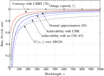
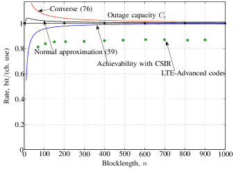
In this section, we compute the bounds reported in Sections IV and V. Fig. 2 compares $R_{\mathrm{rt}}^{\mathcal{N}}(n,\epsilon)$ with the achievability bound (67) and the converse bound (76) for a quasi-static SIMO fading channel with two receive antennas. The channels between the transmit antenna and each of the two receive antennas are Rician-distributed with $K$-factor equal to $20$ dB. The two channels are assumed to be independent. We set $\epsilon=10^{-3}$ and choose $\rho=-1.55$ dB so that $C_{\epsilon}=1$ bit$/$(ch. use). We also plot a lower bound on $R_{\mathrm{rt}}^{\ast}(n,\epsilon)$ obtained by using the $\kappa\beta$ bound [9, Th. 25] and assuming CSIR.777Specifically, we took ={𝒙\use@mathgroup\M@U\symAMSbCn:𝒙2=nρ}conditional-set𝒙\use@mathgroup\M@U\symAMSbsuperscript𝐶𝑛superscriptnorm𝒙2𝑛𝜌\mathcal{F}=\{\bm{x}\in\use@mathgroup\M@U\symAMSb{C}^{n}:\|\bm{x}\|^{2}=n\rho\}, and Q\use@mathgroup\M@U\symAMSbY𝑯=P𝑯j=1nQ𝒀j|𝑯subscript𝑄\use@mathgroup\M@U\symAMSb𝑌𝑯subscript𝑃𝑯superscriptsubscriptproduct𝑗1𝑛subscript𝑄conditionalsubscript𝒀𝑗𝑯Q_{\use@mathgroup\M@U\symAMSb{Y}\bm{H}}=P_{\bm{H}}\prod\nolimits_{j=1}^{n}Q_{\bm{Y}_{j}\,|\,\bm{H}} where $Q_{\bm{Y}_{j}\,|\,\bm{H}=\bm{h}}=\mathcal{CN}(\mathbf{0},\mathsf{I}_{r}+\rho\bm{h}\bm{h}^{\mathrm{H}})$. For reference, Fig. 2 shows also the approximation (2) for $R^{\ast}(n,\epsilon)$ corresponding to an AWGN channel with $C=1$ bit$/$(ch. use), replacing the term $\mathcal{O}(\log(n)/n)$ in (2) with $\log(n)/(2n)$ [9, Eq. (296)][30].888The approximation reported in [9, Eq. (296)],[30] holds for a real AWGN channel. Since a complex AWGN channel with blocklength $n$ can be identified as a real AWGN channel with the same SNR and blocklength $2n$, the approximation [9, Eq. (296)],[30] with $C=\log(1+\rho)$ and $V=\frac{\rho^{2}+2\rho}{(1+\rho)^{2}}$ is accurate for the complex case. The blocklength required to achieve $90\%$ of the $\epsilon$-capacity of the quasi-static fading channel is in the range $[120,320]$ for the CSIRT case and in the range $[120,480]$ for the no-CSI case. For the AWGN channel, this number is approximately $1420$. Hence, for the parameters chosen in Fig. 2, the prediction (based on zero dispersion) of fast convergence to capacity is validated. The gap between the normal approximation $R_{\mathrm{rt}}^{\mathcal{N}}(n,\epsilon)$ defined implicitly in (59) and both the achievability (CSIR) and the converse bounds is less than $0.02$ bit$/$(ch. use) for blocklengths larger than $400$.

Note that although the AWGN curve in Fig. 2 lies below the achievability bound for the quasi-static fading channel, this does not mean that “fading helps”. In Fig. 2, we chose the SNRs so that both channels have the same $\epsilon$-capacity. This results in the received power for the quasi-static case being $1.45$ dB larger than that for the AWGN case.

Refer to caption
Figure 3: Achievability and converse bounds for $(n,M,\epsilon)_{\mathrm{iso}}$ codes over a quasi-static MIMO Rayleigh-fading channel with two transmit and three receive antennas, $\text{SNR}=2.12$ dB, and $\epsilon=10^{-3}$.

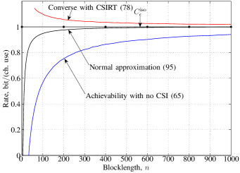
In Fig. 3, we compare the normal approximation $R_{\mathrm{rx},\mathrm{iso}}^{\mathcal{N}}(n,\epsilon)$ defined (implicitly) in (95) with the achievability bound (65) and the converse bound (78) on the maximal achievable rate with $(n,M,\epsilon)_{\mathrm{iso}}$ codes over a quasi-static MIMO fading channel with $t=2$ transmit and $r=3$ receive antennas. The channel between each transmit-receive antenna pair is Rayleigh-distributed, and the channels between different transmit-receive antenna pairs are assumed to be independent. We set $\epsilon=10^{-3}$ and choose $\rho=2.12$ dB so that $C_{\epsilon}^{\mathrm{iso}}=1$ bit$/$(ch. use). For this scenario, the blocklength required to achieve $90\%$ of $C_{\epsilon}^{\mathrm{iso}}$ is less than $500$, which again demonstrates fast convergence to $C_{\epsilon}^{\mathrm{iso}}$.

VI-B Comparison with coding schemes in LTE-Advanced

The bounds reported in Sections IV and V can be used to benchmark the coding schemes adopted in current standards. In Fig. 4, we compare the performance of the coding schemes used in LTE-Advanced [31, Sec. 5.1.3.2] against the achievability and converse bounds for the same scenario as in Fig. 2. Specifically, Fig. 4 illustrates the performance of the family of turbo codes chosen in LTE-Advanced for the case of QPSK modulation. The decoder employs a max-log-MAP decoding algorithm [32] with 10 iterations. We further assume that the decoder has perfect CSI. For the AWGN case, it was observed in [9, Fig. 12] that about half of the gap between the rate achieved by the best available channel codes999The codes used in [9, Fig. 12] are a certain family of multiedge low-density parity-check (LDPC) codes. and capacity is due to the $1/\sqrt{n}$ penalty in (2); the other half is due to the suboptimality of the codes. From Fig. 4, we conclude that for quasi-static fading channels the finite-blocklength penalty is significantly reduced because of the zero-dispersion effect. However, the penalty due to the code suboptimality remains. In fact, we see that the gap between the rate achieved by the LTE-Advanced turbo codes and the normal approximation $R_{\mathrm{rt}}^{\mathcal{N}}(n,\epsilon)$ is approximately constant up to a blocklength of $1000$.

Refer to caption
Figure 4: Comparison between achievability and converse bounds and the rate achievable with the coding schemes in LTE-Advanced. We consider a quasi-static SIMO Rician-fading channel with $K$-factor equal to $20$ dB, two receive antennas, $\text{SNR}=-1.55$ dB, $\epsilon=10^{-3}$, and CSIR. The star-shaped markers indicate the rates achievable by the turbo codes in LTE-Advanced (QPSK modulation and 10 iterations of a max-log-MAP decoder [32]).
Refer to caption
Figure 5: Comparison between achievability and converse bounds and rate achievable with the coding schemes in LTE-Advanced. We consider a quasi-static SIMO Rayleigh-fading channel with two receive antennas, $\text{SNR}=2.74$ dB, $\epsilon=0.1$, and CSIR. The star-shaped markers indicate the rates achievable by the turbo codes in LTE-Advanced (QPSK modulation and 10 iterations of a max-log-MAP decoder [32]).

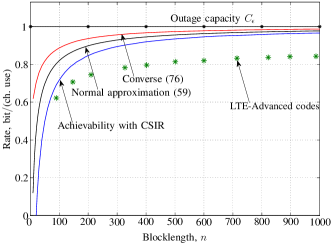
LTE-Advanced uses hybrid automatic repeat request (HARQ) to compensate for packets loss due to outage events. When HARQ is used, the block error rate that maximizes the average throughput is about $10^{-1}$ [33, p. 218]. The performance of LTE-Advanced codes for $\epsilon=10^{-1}$ is analyzed in Fig. 5. We set $\rho=2.74$ dB and consider Rayleigh fading (the other parameters are as in Fig. 4). Again, we observe that there is a constant gap between the rate achieved by LTE-Advanced turbo codes and $R_{\mathrm{rt}}^{\mathcal{N}}(n,\epsilon)$.

VII Conclusion

In this paper, we established achievability and converse bounds on the maximal achievable rate $R^{\ast}(n,\epsilon)$ for a given blocklength $n$ and error probability $\epsilon$ over quasi-static MIMO fading channels. We proved that (under some mild conditions on the fading distribution) the channel dispersion is zero for all four cases of CSI availability. The bounds are easy to evaluate when CSIT is available, when the number of transmit antennas is one, or when the code has isotropic codewords. In all these cases the outage-capacity-achieving distribution is known.

The numerical results reported in Section VI-A demonstrate that, in some scenarios, zero dispersion implies fast convergence to $C_{\epsilon}$ as the blocklength increases. This suggests that the outage capacity is a valid performance metric for communication systems with stringent latency constraints operating over quasi-static fading channels. We developed an easy-to-evaluate approximation of $R^{\ast}(n,\epsilon)$ and demonstrated its accuracy by comparison to our achievability and converse bounds. Finally, we used our bounds to benchmark the performance of the coding schemes adopted in the LTE-Advanced standard. Specifically, we showed that for a blocklength between $500$ and $1000$ LTE-Advanced codes achieve about $85\%$ of the maximal coding rate.

Appendix A Auxiliary Lemmas Concerning the Product of Sines of Principal Angles

In this appendix, we state two properties of the product of principal sines defined in (40), which will be used in the proof of Theorem 3 and of Proposition 23. The first property, which is referred to in [34] as “equalized Hadamard inequality”, is stated in Lemma 12 below.

Lemma 12

Let 𝖠=[𝖠1,𝖠2]\use@mathgroup\M@U\symAMSbCn×(a1+a2)𝖠subscript𝖠1subscript𝖠2\use@mathgroup\M@U\symAMSbsuperscript𝐶𝑛subscript𝑎1subscript𝑎2\mathsf{A}=[\mathsf{A}_{1},\mathsf{A}_{2}]\in\use@mathgroup\M@U\symAMSb{C}^{n\times(a_{1}+a_{2})}, where 𝖠1\use@mathgroup\M@U\symAMSbCn×a1subscript𝖠1\use@mathgroup\M@U\symAMSbsuperscript𝐶𝑛subscript𝑎1\mathsf{A}_{1}\in\use@mathgroup\M@U\symAMSb{C}^{n\times a_{1}} and 𝖠2\use@mathgroup\M@U\symAMSbCn×a2subscript𝖠2\use@mathgroup\M@U\symAMSbsuperscript𝐶𝑛subscript𝑎2\mathsf{A}_{2}\in\use@mathgroup\M@U\symAMSb{C}^{n\times a_{2}}. If $\mathrm{rank}(\mathsf{A}_{1})=a_{1}$ and $\mathrm{rank}(\mathsf{A}_{2})=a_{2}$, then

$\displaystyle\det(\mathsf{A}^{\mathrm{H}}\mathsf{A})=\det(\mathsf{A}_{1}^{\mathrm{H}}\mathsf{A}_{1})\det(\mathsf{A}_{2}^{\mathrm{H}}\mathsf{A}_{2})\sin^{2}\{\mathsf{A}_{1},\mathsf{A}_{2}\}.$ (98)
Proof:

The proof follows by extending [35, Th. 3.3] to the complex case. ∎

The second property provides an upper bound on $\sin\{\mathcal{A},\mathcal{B}\}$ that depends on the angles between the basis vectors of the two subspaces.

Lemma 13

Let $\mathcal{A}$ and $\mathcal{B}$ be subspaces of \use@mathgroup\M@U\symAMSbCn\use@mathgroup\M@U\symAMSbsuperscript𝐶𝑛\use@mathgroup\M@U\symAMSb{C}^{n} with $\dim(\mathcal{A})=a$ and $\dim(\mathcal{B})=b$. Let $\{\bm{a}_{1},\ldots,\bm{a}_{a}\}$ be an orthonormal basis for $\mathcal{A}$, and let $\{\bm{b}_{1},\ldots,\bm{b}_{b}\}$ be an arbitrary basis (not necessarily orthonormal) for $\mathcal{B}$. Then

$\displaystyle\sin\{\mathcal{A},\mathcal{B}\}\leq\prod\limits^{\min\{a,b\}}_{j=1}\sin\{\bm{a}_{j},\bm{b}_{j}\}.$ (99)
Proof:

To keep notation simple, we define the following function, which maps a complex matrix $\mathsf{X}$ of arbitrary size to its volume:

$\displaystyle\mathrm{vol}(\mathsf{X})\triangleq\sqrt{\det(\mathsf{X}^{\mathrm{H}}\mathsf{X})}.$ (100)

Let 𝖠=[𝒂1,,𝒂a]\use@mathgroup\M@U\symAMSbCn×a𝖠subscript𝒂1subscript𝒂𝑎\use@mathgroup\M@U\symAMSbsuperscript𝐶𝑛𝑎\mathsf{A}=[\bm{a}_{1},\ldots,\bm{a}_{a}]\in\use@mathgroup\M@U\symAMSb{C}^{n\times a} and 𝖡=[𝒃1,,𝒃b]\use@mathgroup\M@U\symAMSbCn×b𝖡subscript𝒃1subscript𝒃𝑏\use@mathgroup\M@U\symAMSbsuperscript𝐶𝑛𝑏\mathsf{B}=[\bm{b}_{1},\ldots,\bm{b}_{b}]\in\use@mathgroup\M@U\symAMSb{C}^{n\times b}. If the vectors $\bm{a}_{1},\ldots,\bm{a}_{a},\bm{b}_{1},\ldots,\bm{b}_{b}$ are linearly dependent, then the LHS of (99) vanishes, in which case (99) holds trivially. In the following, we therefore assume that the vectors $\bm{a}_{1},\ldots,\bm{a}_{a},\bm{b}_{1},\ldots,\bm{b}_{b}$ form a linearly independent set. Below, we prove Lemma 13 for the case $a\leq b$. The proof for the case $a>b$ follows from similar steps.

Using Lemma 12, we get the following chain of (in)equalities:

$\displaystyle\IEEEeqnarraymulticol{3}{l}{\sin\{\mathsf{A},\mathsf{B}\}}$ (101)
$\displaystyle=$ $\displaystyle\frac{\mathrm{vol}([\mathsf{A},\mathsf{B}])}{\mathrm{vol}(\mathsf{A})\mathrm{vol}(\mathsf{B})}$
$\displaystyle=$ $\displaystyle\frac{\mathrm{vol}([\mathsf{A},\mathsf{B}])}{\mathrm{vol}(\mathsf{B})}$
$\displaystyle=$ $\displaystyle\frac{1}{\mathrm{vol}(\mathsf{B})}\underbrace{\|\bm{a}_{1}\|}_{=1}\mathrm{vol}\mathopen{}\big{(}[\bm{a}_{2},\ldots,\bm{a}_{a},\mathsf{B}]\big{)}$
$\displaystyle\cdot\,\sin\mathopen{}\big{\{}\bm{a}_{1},[\bm{a}_{2},\ldots,\bm{a}_{a},\mathsf{B}]\big{\}}$
$\displaystyle\vdots$
$\displaystyle=$ $\displaystyle\frac{1}{\mathrm{vol}(\mathsf{B})}\left(\prod\limits_{i=1}^{a}\sin\mathopen{}\big{\{}\bm{a}_{i},[\bm{a}_{i+1},\ldots,\bm{a}_{a},\mathsf{B}]\big{\}}\!\right)\mathrm{vol}(\mathsf{B})\quad$ (104)
$\displaystyle\leq$ $\displaystyle\prod\limits_{i=1}^{a}\sin\{\bm{a}_{i},\bm{b}_{i}\}.$ (105)

Here, (A) holds because the columns of $\mathsf{A}$ are orthonormal and, hence, $\det(\mathsf{A}^{\mathrm{H}}\mathsf{A})=1$; (A) and (104) follow from Lemma 12; (105) follows because

$\displaystyle\sin\mathopen{}\big{\{}\bm{a}_{i},[\bm{a}_{i+1},\ldots,\bm{a}_{a},\mathsf{B}]\big{\}}\leq\sin\{\bm{a}_{i},\bm{b}_{i}\}.$ (106)

Appendix B Proof of Theorem 1 (CSIT Achievability Bound)

Given \use@mathgroup\M@U\symAMSbH=𝖧\use@mathgroup\M@U\symAMSb𝐻𝖧\use@mathgroup\M@U\symAMSb{H}=\mathsf{H}, we perform a singular value decomposition (SVD) of $\mathsf{H}$ to obtain

$\displaystyle\mathsf{H}=\mathsf{L}\mathsf{\Sigma}\mathsf{V}^{\mathrm{H}}$ (107)

where 𝖫\use@mathgroup\M@U\symAMSbCt×t𝖫\use@mathgroup\M@U\symAMSbsuperscript𝐶𝑡𝑡\mathsf{L}\in\use@mathgroup\M@U\symAMSb{C}^{t\times t} and 𝖵\use@mathgroup\M@U\symAMSbCr×r𝖵\use@mathgroup\M@U\symAMSbsuperscript𝐶𝑟𝑟\mathsf{V}\in\use@mathgroup\M@U\symAMSb{C}^{r\times r} are unitary matrices, and Σ\use@mathgroup\M@U\symAMSbCt×rsans-serif-Σ\use@mathgroup\M@U\symAMSbsuperscript𝐶𝑡𝑟\mathsf{\Sigma}\in\use@mathgroup\M@U\symAMSb{C}^{t\times r} is a (truncated) diagonal matrix of dimension $t\times r$, whose diagonal elements $\sqrt{\lambda_{1}},\ldots,\sqrt{\lambda_{m}}$, are the ordered singular values of $\mathsf{H}$. It will be convenient to define the following $t\times t$ precoding matrix for each $\mathsf{H}$:

$\displaystyle\mathsf{P}(\mathsf{H})\triangleq\mathrm{diag}\{\sqrt{nv^{\ast}_{1}},\ldots,\sqrt{nv^{\ast}_{m}},\underbrace{0,\ldots,0}_{t-m}\}\mathsf{L}^{\mathrm{H}}.$ (108)

We consider a code whose codewords 𝖷j(\use@mathgroup\M@U\symAMSbH)subscript𝖷𝑗\use@mathgroup\M@U\symAMSb𝐻\mathsf{X}_{j}(\use@mathgroup\M@U\symAMSb{H}), $j=1,\ldots,M$, have the following structure

𝖷j(\use@mathgroup\M@U\symAMSbH)=Φj𝖯(\use@mathgroup\M@U\symAMSbH),Φj𝒮n,tformulae-sequencesubscript𝖷𝑗\use@mathgroup\M@U\symAMSb𝐻subscriptsans-serif-Φ𝑗𝖯\use@mathgroup\M@U\symAMSb𝐻subscriptsans-serif-Φ𝑗subscript𝒮𝑛𝑡\displaystyle\mathsf{X}_{j}(\use@mathgroup\M@U\symAMSb{H})=\mathsf{\Phi}_{j}\mathsf{P}(\use@mathgroup\M@U\symAMSb{H}),\quad\mathsf{\Phi}_{j}\in\mathcal{S}_{n,t} (109)

where 𝒮n,t{𝖠\use@mathgroup\M@U\symAMSbCn×t:𝖠H𝖠=𝖨t}subscript𝒮𝑛𝑡conditional-set𝖠\use@mathgroup\M@U\symAMSbsuperscript𝐶𝑛𝑡superscript𝖠H𝖠subscript𝖨𝑡\mathcal{S}_{n,t}\triangleq\{\mathsf{A}\in\use@mathgroup\M@U\symAMSb{C}^{n\times t}:\mathsf{A}^{\mathrm{H}}\mathsf{A}=\mathsf{I}_{t}\} denotes the set of all $n\times t$ unitary matrices, (i.e., the complex Stiefel manifold). As $\{\mathsf{\Phi}_{j}\}$ are unitary, the codewords satisfy the power constraint (12). Motivated by the geometric considerations reported in Section IV-A1, we consider for a given input 𝖷(\use@mathgroup\M@U\symAMSbH)=Φ𝖯(\use@mathgroup\M@U\symAMSbH)𝖷\use@mathgroup\M@U\symAMSb𝐻sans-serif-Φ𝖯\use@mathgroup\M@U\symAMSb𝐻\mathsf{X}(\use@mathgroup\M@U\symAMSb{H})=\mathsf{\Phi}\mathsf{P}(\use@mathgroup\M@U\symAMSb{H}) a physically degraded version of the channel (8), whose output is given by

Ω\use@mathgroup\M@U\symAMSbY=span(Φ𝖯(\use@mathgroup\M@U\symAMSbH)\use@mathgroup\M@U\symAMSbH+\use@mathgroup\M@U\symAMSbW).subscriptΩ\use@mathgroup\M@U\symAMSb𝑌spansans-serif-Φ𝖯\use@mathgroup\M@U\symAMSb𝐻\use@mathgroup\M@U\symAMSb𝐻\use@mathgroup\M@U\symAMSb𝑊\displaystyle\Omega_{\use@mathgroup\M@U\symAMSb{Y}}=\mathrm{span}(\mathsf{\Phi}\mathsf{P}(\use@mathgroup\M@U\symAMSb{H})\use@mathgroup\M@U\symAMSb{H}+\use@mathgroup\M@U\symAMSb{W}). (110)

Note that the subspace Ω\use@mathgroup\M@U\symAMSbYsubscriptΩ\use@mathgroup\M@U\symAMSb𝑌\Omega_{\use@mathgroup\M@U\symAMSb{Y}} belongs with probability one to the Grassmannian manifold $\mathcal{G}_{n,r}$, i.e., the set of all $r$ dimensional subspaces in \use@mathgroup\M@U\symAMSbCn\use@mathgroup\M@U\symAMSbsuperscript𝐶𝑛\use@mathgroup\M@U\symAMSb{C}^{n}. Because (110) is a physically degraded version of (8), the rate achievable on (110) is a lower bound on the rate achievable on (8).

To prove the theorem, we apply the $\kappa\beta$ bound [9, Th. 25] to the channel (110). Following [9, Eq. (107)], we define the following measure of performance for the composite hypothesis test between an auxiliary output distribution QΩ\use@mathgroup\M@U\symAMSbYsubscript𝑄subscriptΩ\use@mathgroup\M@U\symAMSb𝑌Q_{\Omega_{\use@mathgroup\M@U\symAMSb{Y}}} defined on the subspace Ω\use@mathgroup\M@U\symAMSbYsubscriptΩ\use@mathgroup\M@U\symAMSb𝑌\Omega_{\use@mathgroup\M@U\symAMSb{Y}} and the collection of channel-output distributions {PΩ\use@mathgroup\M@U\symAMSbY|Φ=Φ}Φ𝒮n,tsubscriptsubscript𝑃conditionalsubscriptΩ\use@mathgroup\M@U\symAMSb𝑌double-struck-Φsans-serif-Φsans-serif-Φsubscript𝒮𝑛𝑡\{P_{\Omega_{\use@mathgroup\M@U\symAMSb{Y}}\,|\,\mathbb{\Phi}=\mathsf{\Phi}}\}_{\mathsf{\Phi}\in\mathcal{S}_{n,t}}:

κτ(𝒮n,t,QΩ\use@mathgroup\M@U\symAMSbY)infPZ|Ω\use@mathgroup\M@U\symAMSbY(1|Ω𝖸)QΩ\use@mathgroup\M@U\symAMSbY(dΩ𝖸)subscript𝜅𝜏subscript𝒮𝑛𝑡subscript𝑄subscriptΩ\use@mathgroup\M@U\symAMSb𝑌infimumsubscript𝑃conditional𝑍subscriptΩ\use@mathgroup\M@U\symAMSb𝑌conditional1subscriptΩ𝖸subscript𝑄subscriptΩ\use@mathgroup\M@U\symAMSb𝑌𝑑subscriptΩ𝖸\displaystyle\kappa_{\tau}(\mathcal{S}_{n,t},Q_{\Omega_{\use@mathgroup\M@U\symAMSb{Y}}})\triangleq\inf\int P_{Z\,|\,\Omega_{\use@mathgroup\M@U\symAMSb{Y}}}(1\,|\,\Omega_{\mathsf{Y}})Q_{\Omega_{\use@mathgroup\M@U\symAMSb{Y}}}(d\Omega_{\mathsf{Y}}) (111)

where the infimum is over all probability distributions PZ|Ω\use@mathgroup\M@U\symAMSbY:𝒢n,t{0,1}:subscript𝑃conditional𝑍subscriptΩ\use@mathgroup\M@U\symAMSb𝑌maps-tosubscript𝒢𝑛𝑡01P_{Z\,|\,\Omega_{\use@mathgroup\M@U\symAMSb{Y}}}:\mathcal{G}_{n,t}\mapsto\{0,1\} satisfying

PZ|Ω\use@mathgroup\M@U\symAMSbY(1|Ω𝖸)PΩ\use@mathgroup\M@U\symAMSbY|Φ=Φ(dΩ𝖸)τ,Φ𝒮n,t.formulae-sequencesubscript𝑃conditional𝑍subscriptΩ\use@mathgroup\M@U\symAMSb𝑌conditional1subscriptΩ𝖸subscript𝑃conditionalsubscriptΩ\use@mathgroup\M@U\symAMSb𝑌double-struck-Φsans-serif-Φ𝑑subscriptΩ𝖸𝜏for-allsans-serif-Φsubscript𝒮𝑛𝑡\displaystyle\,\int P_{Z\,|\,\Omega_{\use@mathgroup\M@U\symAMSb{Y}}}(1\,|\,\Omega_{\mathsf{Y}})P_{\Omega_{\use@mathgroup\M@U\symAMSb{Y}}\,|\,\mathbb{\Phi}=\mathsf{\Phi}}(d\Omega_{\mathsf{Y}})\geq\tau,\quad\forall\mathsf{\Phi}\in\mathcal{S}_{n,t}. (112)

By [9, Th. 25], we have that for every auxiliary distribution QΩ\use@mathgroup\M@U\symAMSbYsubscript𝑄subscriptΩ\use@mathgroup\M@U\symAMSb𝑌Q_{\Omega_{\use@mathgroup\M@U\symAMSb{Y}}}

Mκτ(𝒮n,t,QΩ\use@mathgroup\M@U\symAMSbY)supΦ𝒮n,tβ1ϵ+τ(PΩ\use@mathgroup\M@U\symAMSbY|Φ=Φ,QΩ\use@mathgroup\M@U\symAMSbY)𝑀subscript𝜅𝜏subscript𝒮𝑛𝑡subscript𝑄subscriptΩ\use@mathgroup\M@U\symAMSb𝑌subscriptsupremumsans-serif-Φsubscript𝒮𝑛𝑡subscript𝛽1italic-ϵ𝜏subscript𝑃conditionalsubscriptΩ\use@mathgroup\M@U\symAMSb𝑌double-struck-Φsans-serif-Φsubscript𝑄subscriptΩ\use@mathgroup\M@U\symAMSb𝑌\displaystyle M\geq\frac{\kappa_{\tau}(\mathcal{S}_{n,t},Q_{\Omega_{\use@mathgroup\M@U\symAMSb{Y}}})}{\sup_{\mathsf{\Phi}\in\mathcal{S}_{n,t}}\beta_{1-\epsilon+\tau}(P_{\Omega_{\use@mathgroup\M@U\symAMSb{Y}}\,|\,\mathbb{\Phi}=\mathsf{\Phi}},Q_{\Omega_{\use@mathgroup\M@U\symAMSb{Y}}})} (113)

where $\beta_{(\cdot)}(\cdot,\cdot)$ is defined in (6). We next lower-bound the RHS of (113) to obtain an expression that can be evaluated numerically. Fix a $\mathsf{\Phi}\in\mathcal{S}_{n,t}$ and let

ZΦ(Ω\use@mathgroup\M@U\symAMSbY)subscript𝑍sans-serif-ΦsubscriptΩ\use@mathgroup\M@U\symAMSb𝑌\displaystyle Z_{\mathsf{\Phi}}(\Omega_{\use@mathgroup\M@U\symAMSb{Y}}) $\displaystyle=$ 𝟙{sin2{span(Φ),Ω\use@mathgroup\M@U\symAMSbY}γn}1superscript2spansans-serif-ΦsubscriptΩ\use@mathgroup\M@U\symAMSb𝑌subscript𝛾𝑛\displaystyle\mathbbmss{1}\{\sin^{2}\{\mathrm{span}(\mathsf{\Phi}),\Omega_{\use@mathgroup\M@U\symAMSb{Y}}\}\leq\gamma_{n}\} (114)

where $\gamma_{n}\in[0,1]$ is chosen so that

PΩ\use@mathgroup\M@U\symAMSbY|Φ=Φ[ZΦ(Ω\use@mathgroup\M@U\symAMSbY)=1]1ϵ+τ.subscript𝑃conditionalsubscriptΩ\use@mathgroup\M@U\symAMSb𝑌double-struck-Φsans-serif-Φdelimited-[]subscript𝑍sans-serif-ΦsubscriptΩ\use@mathgroup\M@U\symAMSb𝑌11italic-ϵ𝜏\displaystyle P_{\Omega_{\use@mathgroup\M@U\symAMSb{Y}}|\mathbb{\Phi}=\mathsf{\Phi}}[Z_{\mathsf{\Phi}}(\Omega_{\use@mathgroup\M@U\symAMSb{Y}})=1]\geq 1-\epsilon+\tau. (115)

Since the noise matrix \use@mathgroup\M@U\symAMSbW\use@mathgroup\M@U\symAMSb𝑊\use@mathgroup\M@U\symAMSb{W} is isotropically distributed, the probability distribution of the random variable sin2{span(Φ),Ω\use@mathgroup\M@U\symAMSbY}superscript2spansans-serif-ΦsubscriptΩ\use@mathgroup\M@U\symAMSb𝑌\sin^{2}\{\mathrm{span}(\mathsf{\Phi}),\Omega_{\use@mathgroup\M@U\symAMSb{Y}}\} (where Ω\use@mathgroup\M@U\symAMSbYPΩ\use@mathgroup\M@U\symAMSbY|Φ=Φsimilar-tosubscriptΩ\use@mathgroup\M@U\symAMSb𝑌subscript𝑃conditionalsubscriptΩ\use@mathgroup\M@U\symAMSb𝑌double-struck-Φsans-serif-Φ\Omega_{\use@mathgroup\M@U\symAMSb{Y}}\sim P_{\Omega_{\use@mathgroup\M@U\symAMSb{Y}}|\mathbb{\Phi}=\mathsf{\Phi}}) does not depend on $\mathsf{\Phi}$. Hence, the chosen $\gamma_{n}$ satisfies (115) for all $\mathsf{\Phi}\in\mathcal{S}_{n,t}$. Furthermore, ZΦ(Ω\use@mathgroup\M@U\symAMSbY)subscript𝑍sans-serif-ΦsubscriptΩ\use@mathgroup\M@U\symAMSb𝑌Z_{\mathsf{\Phi}}(\Omega_{\use@mathgroup\M@U\symAMSb{Y}}) can be viewed as a hypothesis test between PΩ\use@mathgroup\M@U\symAMSbY|Φ=Φsubscript𝑃conditionalsubscriptΩ\use@mathgroup\M@U\symAMSb𝑌double-struck-Φsans-serif-ΦP_{\Omega_{\use@mathgroup\M@U\symAMSb{Y}}\,|\,\mathbb{\Phi}=\mathsf{\Phi}} and QΩ\use@mathgroup\M@U\symAMSbYsubscript𝑄subscriptΩ\use@mathgroup\M@U\symAMSb𝑌Q_{\Omega_{\use@mathgroup\M@U\symAMSb{Y}}}. Hence, by definition

β1ϵ+τ(PΩ\use@mathgroup\M@U\symAMSbY|Φ=Φ,QΩ\use@mathgroup\M@U\symAMSbY)QΩ\use@mathgroup\M@U\symAMSbY[ZΦ(Ω\use@mathgroup\M@U\symAMSbY)=1]subscript𝛽1italic-ϵ𝜏subscript𝑃conditionalsubscriptΩ\use@mathgroup\M@U\symAMSb𝑌double-struck-Φsans-serif-Φsubscript𝑄subscriptΩ\use@mathgroup\M@U\symAMSb𝑌subscript𝑄subscriptΩ\use@mathgroup\M@U\symAMSb𝑌delimited-[]subscript𝑍sans-serif-ΦsubscriptΩ\use@mathgroup\M@U\symAMSb𝑌1\displaystyle\beta_{1-\epsilon+\tau}(P_{\Omega_{\use@mathgroup\M@U\symAMSb{Y}}\,|\,\mathbb{\Phi}=\mathsf{\Phi}},Q_{\Omega_{\use@mathgroup\M@U\symAMSb{Y}}})\leq Q_{\Omega_{\use@mathgroup\M@U\symAMSb{Y}}}[Z_{\mathsf{\Phi}}(\Omega_{\use@mathgroup\M@U\symAMSb{Y}})=1] (116)

for every $\mathsf{\Phi}\in\mathcal{S}_{n,t}$.

We next evaluate the RHS of (116), taking as the auxiliary output distribution the uniform distribution on $\mathcal{G}_{n,r}$, which we denote by QΩ\use@mathgroup\M@U\symAMSbYusubscriptsuperscript𝑄usubscriptΩ\use@mathgroup\M@U\symAMSb𝑌Q^{\mathrm{u}}_{\Omega_{\use@mathgroup\M@U\symAMSb{Y}}}. With this choice, QΩ\use@mathgroup\M@U\symAMSbYu[sin2{span(Φ),Ω\use@mathgroup\M@U\symAMSbY}γn]subscriptsuperscript𝑄usubscriptΩ\use@mathgroup\M@U\symAMSb𝑌delimited-[]superscript2spansans-serif-ΦsubscriptΩ\use@mathgroup\M@U\symAMSb𝑌subscript𝛾𝑛Q^{\mathrm{u}}_{\Omega_{\use@mathgroup\M@U\symAMSb{Y}}}[\sin^{2}\{\mathrm{span}(\mathsf{\Phi}),\Omega_{\use@mathgroup\M@U\symAMSb{Y}}\}\leq\gamma_{n}] does not depend on $\mathsf{\Phi}\in\mathcal{S}_{n,t}$. To simplify calculations, we can therefore set $\mathsf{\Phi}=\mathsf{I}_{n,t}$. Observe that under QΩ\use@mathgroup\M@U\symAMSbYusubscriptsuperscript𝑄usubscriptΩ\use@mathgroup\M@U\symAMSb𝑌Q^{\mathrm{u}}_{\Omega_{\use@mathgroup\M@U\symAMSb{Y}}}, the squares of the sines of the principle angles between $\mathrm{span}(\mathsf{I}_{n,t})$ and Ω\use@mathgroup\M@U\symAMSbYsubscriptΩ\use@mathgroup\M@U\symAMSb𝑌\Omega_{\use@mathgroup\M@U\symAMSb{Y}} have the same distribution as the eigenvalues of a complex multivariate Beta-distributed matrix \use@mathgroup\M@U\symAMSbBBetar(nt,t)similar-to\use@mathgroup\M@U\symAMSb𝐵subscriptBeta𝑟𝑛𝑡𝑡\use@mathgroup\M@U\symAMSb{B}\sim\mathrm{Beta}_{r}(n-t,t) [36, Sec. 2]. By [37, Cor. 1], the distribution of det\use@mathgroup\M@U\symAMSbB\use@mathgroup\M@U\symAMSb𝐵\det\use@mathgroup\M@U\symAMSb{B} coincides with the distribution of $\prod_{i=1}^{r}B_{i}$, where $\{B_{i}\}$, ${i=1,\ldots,r}$, are independent with $B_{i}\sim\mathrm{Beta}(n-t-i+1,t)$. Using this result to compute the RHS of (116) we obtain

supΦ𝒮n,tβ1ϵ+τ(PΩ\use@mathgroup\M@U\symAMSbY|Φ=Φ,QΩ\use@mathgroup\M@U\symAMSbY)\use@mathgroup\M@U\symAMSbP[j=1rBjγn]subscriptsupremumsans-serif-Φsubscript𝒮𝑛𝑡subscript𝛽1italic-ϵ𝜏subscript𝑃conditionalsubscriptΩ\use@mathgroup\M@U\symAMSb𝑌double-struck-Φsans-serif-Φsubscript𝑄subscriptΩ\use@mathgroup\M@U\symAMSb𝑌\use@mathgroup\M@U\symAMSb𝑃delimited-[]superscriptsubscriptproduct𝑗1𝑟subscript𝐵𝑗subscript𝛾𝑛\displaystyle\sup_{\mathsf{\Phi}\in\mathcal{S}_{n,t}}\beta_{1-\epsilon+\tau}(P_{\Omega_{\use@mathgroup\M@U\symAMSb{Y}}\,|\,\mathbb{\Phi}=\mathsf{\Phi}},Q_{\Omega_{\use@mathgroup\M@U\symAMSb{Y}}})\leq\use@mathgroup\M@U\symAMSb{P}\mathopen{}\left[\prod_{j=1}^{r}B_{j}\leq\gamma_{n}\right] (117)

where $\gamma_{n}$ satisfies

\use@mathgroup\M@U\symAMSbP[sin2{𝖨n,t,𝖨n,t𝖯(\use@mathgroup\M@U\symAMSbH)\use@mathgroup\M@U\symAMSbH+\use@mathgroup\M@U\symAMSbW}γn]1ϵ+τ.\use@mathgroup\M@U\symAMSb𝑃delimited-[]superscript2subscript𝖨𝑛𝑡subscript𝖨𝑛𝑡𝖯\use@mathgroup\M@U\symAMSb𝐻\use@mathgroup\M@U\symAMSb𝐻\use@mathgroup\M@U\symAMSb𝑊subscript𝛾𝑛1italic-ϵ𝜏\displaystyle\use@mathgroup\M@U\symAMSb{P}\mathopen{}\Big{[}\sin^{2}\mathopen{}\big{\{}\mathsf{I}_{n,t},\mathsf{I}_{n,t}\mathsf{P}(\use@mathgroup\M@U\symAMSb{H})\use@mathgroup\M@U\symAMSb{H}+\use@mathgroup\M@U\symAMSb{W}\big{\}}\leq\gamma_{n}\Big{]}\geq 1-\epsilon+\tau. (118)

Note that (118) is equivalent to (44). Indeed

\IEEEeqnarraymulticol3l\use@mathgroup\M@U\symAMSbP[sin2{𝖨n,t,n𝖨n,t𝖯(\use@mathgroup\M@U\symAMSbH)\use@mathgroup\M@U\symAMSbH+\use@mathgroup\M@U\symAMSbW}γn]\IEEEeqnarraymulticol3𝑙\use@mathgroup\M@U\symAMSb𝑃delimited-[]superscript2subscript𝖨𝑛𝑡𝑛subscript𝖨𝑛𝑡𝖯\use@mathgroup\M@U\symAMSb𝐻\use@mathgroup\M@U\symAMSb𝐻\use@mathgroup\M@U\symAMSb𝑊subscript𝛾𝑛\displaystyle\IEEEeqnarraymulticol{3}{l}{\use@mathgroup\M@U\symAMSb{P}\mathopen{}\left[\sin^{2}\mathopen{}\Big{\{}\mathsf{I}_{n,t},\sqrt{n}\mathsf{I}_{n,t}\mathsf{P}(\use@mathgroup\M@U\symAMSb{H})\use@mathgroup\M@U\symAMSb{H}+\use@mathgroup\M@U\symAMSb{W}\Big{\}}\leq\gamma_{n}\right]} (121)
$\displaystyle=$ \use@mathgroup\M@U\symAMSbP[sin2{𝖨n,t,n𝖨n,tdiag{v1Λ1,,vmΛm,\displaystyle\use@mathgroup\M@U\symAMSb{P}\mathopen{}\Big{[}\sin^{2}\mathopen{}\Big{\{}\mathsf{I}_{n,t},\sqrt{n}\mathsf{I}_{n,t}\mathrm{diag}\mathopen{}\big{\{}\sqrt{v_{1}^{\ast}\Lambda_{1}},\ldots,\sqrt{v_{m}^{\ast}\Lambda_{m}},\quad\quad\quad
0,,0tm}\use@mathgroup\M@U\symAMSbVH+\use@mathgroup\M@U\symAMSbW}γn]\displaystyle\hfill\underbrace{0,\ldots,0}_{t-m}\big{\}}\use@mathgroup\M@U\symAMSb{V}^{\mathrm{H}}+\use@mathgroup\M@U\symAMSb{W}\Big{\}}\leq\gamma_{n}\Big{]}
$\displaystyle=$ \use@mathgroup\M@U\symAMSbP[sin2{𝖨n,t,n𝖨n,tdiag{v1Λ1,,vmΛm,\displaystyle\use@mathgroup\M@U\symAMSb{P}\mathopen{}\Big{[}\sin^{2}\mathopen{}\Big{\{}\mathsf{I}_{n,t},\sqrt{n}\mathsf{I}_{n,t}\mathrm{diag}\mathopen{}\big{\{}\sqrt{v_{1}^{\ast}\Lambda_{1}},\ldots,\sqrt{v_{m}^{\ast}\Lambda_{m}},
0,,0tm}+\use@mathgroup\M@U\symAMSbW\use@mathgroup\M@U\symAMSbV}γn]\displaystyle\hfill\underbrace{0,\ldots,0}_{t-m}\big{\}}+\use@mathgroup\M@U\symAMSb{W}\use@mathgroup\M@U\symAMSb{V}\Big{\}}\leq\gamma_{n}\Big{]}
$\displaystyle=$ \use@mathgroup\M@U\symAMSbP[sin2{𝖨n,t,n𝖨n,tdiag{v1Λ1,,vmΛm,\displaystyle\use@mathgroup\M@U\symAMSb{P}\mathopen{}\Big{[}\sin^{2}\mathopen{}\Big{\{}\mathsf{I}_{n,t},\sqrt{n}\mathsf{I}_{n,t}\mathrm{diag}\mathopen{}\big{\{}\sqrt{v_{1}^{\ast}\Lambda_{1}},\ldots,\sqrt{v_{m}^{\ast}\Lambda_{m}},
0,,0tm}+\use@mathgroup\M@U\symAMSbW}γn]\displaystyle\hfill\underbrace{0,\ldots,0}_{t-m}\big{\}}+\use@mathgroup\M@U\symAMSb{W}\Big{\}}\leq\gamma_{n}\Big{]}

where \use@mathgroup\M@U\symAMSbV\use@mathgroup\M@U\symAMSb𝑉\use@mathgroup\M@U\symAMSb{V} contains the right singular vectors of \use@mathgroup\M@U\symAMSbH\use@mathgroup\M@U\symAMSb𝐻\use@mathgroup\M@U\symAMSb{H} (see (107)). Here, (121) follows from (108); (121) follows because right-multiplying a matrix $\mathsf{A}$ by a unitary matrix does not change the subspace spanned by the columns of $\mathsf{A}$ and hence, it does not change $\sin\{\cdot,\cdot\}$; (121) follows because \use@mathgroup\M@U\symAMSbW\use@mathgroup\M@U\symAMSb𝑊\use@mathgroup\M@U\symAMSb{W} is isotropically distributed and hence \use@mathgroup\M@U\symAMSbW\use@mathgroup\M@U\symAMSbV\use@mathgroup\M@U\symAMSb𝑊\use@mathgroup\M@U\symAMSb𝑉\use@mathgroup\M@U\symAMSb{W}\use@mathgroup\M@U\symAMSb{V} has the same distribution as \use@mathgroup\M@U\symAMSbW\use@mathgroup\M@U\symAMSb𝑊\use@mathgroup\M@U\symAMSb{W}.

To conclude the proof, it remains to show that

κτ(𝒮n,t,QΩ\use@mathgroup\M@U\symAMSbYu)τ.subscript𝜅𝜏subscript𝒮𝑛𝑡subscriptsuperscript𝑄usubscriptΩ\use@mathgroup\M@U\symAMSb𝑌𝜏\displaystyle\kappa_{\tau}(\mathcal{S}_{n,t},Q^{\mathrm{u}}_{\Omega_{\use@mathgroup\M@U\symAMSb{Y}}})\geq\tau. (122)

Once this is done, the desired lower bound (43) follows by using the inequality (117) and (122) in (113), by taking the logarithm of both sides of (113), and by dividing by the blocklength $n$.

To prove (122), we replace (112) with the less stringent constraint that

\use@mathgroup\M@U\symAMSbEPΦu[PZ|Ω\use@mathgroup\M@U\symAMSbY(1|Ω𝖸)PΩ\use@mathgroup\M@U\symAMSbY|Φ(dΩ𝖸)]τ\use@mathgroup\M@U\symAMSbsubscript𝐸superscriptsubscript𝑃double-struck-Φudelimited-[]subscript𝑃conditional𝑍subscriptΩ\use@mathgroup\M@U\symAMSb𝑌conditional1subscriptΩ𝖸subscript𝑃conditionalsubscriptΩ\use@mathgroup\M@U\symAMSb𝑌double-struck-Φ𝑑subscriptΩ𝖸𝜏\displaystyle\use@mathgroup\M@U\symAMSb{E}_{P_{\mathbb{\Phi}}^{\mathrm{u}}}\mathopen{}\left[\int P_{Z\,|\,\Omega_{\use@mathgroup\M@U\symAMSb{Y}}}(1\,|\,\Omega_{\mathsf{Y}})P_{\Omega_{\use@mathgroup\M@U\symAMSb{Y}}\,|\,\mathbb{\Phi}}(d\Omega_{\mathsf{Y}})\right]\geq\tau (123)

where $P_{\mathbb{\Phi}}^{\mathrm{u}}$ is the uniform input distribution on $\mathcal{S}_{n,t}$. Since replacing (112) by (123) enlarges the feasible region of the minimization problem (111), we obtain an infimum in (111) (denoted by κτu(𝒮n,t,QΩ\use@mathgroup\M@U\symAMSbYu)subscriptsuperscript𝜅u𝜏subscript𝒮𝑛𝑡subscriptsuperscript𝑄usubscriptΩ\use@mathgroup\M@U\symAMSb𝑌\kappa^{\mathrm{u}}_{\tau}(\mathcal{S}_{n,t},Q^{\mathrm{u}}_{\Omega_{\use@mathgroup\M@U\symAMSb{Y}}})) that is no larger than κτ(𝒮n,t,QΩ\use@mathgroup\M@U\symAMSbYu)subscript𝜅𝜏subscript𝒮𝑛𝑡subscriptsuperscript𝑄usubscriptΩ\use@mathgroup\M@U\symAMSb𝑌\kappa_{\tau}(\mathcal{S}_{n,t},Q^{\mathrm{u}}_{\Omega_{\use@mathgroup\M@U\symAMSb{Y}}}). The key observation is that the uniform distribution $P_{\mathbb{\Phi}}^{\mathrm{u}}$ induces an isotropic distribution on \use@mathgroup\M@U\symAMSbY\use@mathgroup\M@U\symAMSb𝑌\use@mathgroup\M@U\symAMSb{Y}. This implies that the induced distribution on Ω\use@mathgroup\M@U\symAMSbYsubscriptΩ\use@mathgroup\M@U\symAMSb𝑌\Omega_{\use@mathgroup\M@U\symAMSb{Y}} is the uniform distribution on $\mathcal{G}_{n,r}$, i.e., QΩ\use@mathgroup\M@U\symAMSbYusubscriptsuperscript𝑄usubscriptΩ\use@mathgroup\M@U\symAMSb𝑌Q^{\mathrm{u}}_{\Omega_{\use@mathgroup\M@U\symAMSb{Y}}}. Therefore, it follows that

\IEEEeqnarraymulticol3lPZ|Ω\use@mathgroup\M@U\symAMSbY(1|Ω𝖸)QΩ\use@mathgroup\M@U\symAMSbYu(dΩ𝖸)\IEEEeqnarraymulticol3𝑙subscript𝑃conditional𝑍subscriptΩ\use@mathgroup\M@U\symAMSb𝑌conditional1subscriptΩ𝖸subscriptsuperscript𝑄usubscriptΩ\use@mathgroup\M@U\symAMSb𝑌𝑑subscriptΩ𝖸\displaystyle\IEEEeqnarraymulticol{3}{l}{\int P_{Z\,|\,\Omega_{\use@mathgroup\M@U\symAMSb{Y}}}(1\,|\,\Omega_{\mathsf{Y}})Q^{\mathrm{u}}_{\Omega_{\use@mathgroup\M@U\symAMSb{Y}}}(d\Omega_{\mathsf{Y}})}
$\displaystyle=$ \use@mathgroup\M@U\symAMSbEPΦu[PZ|Ω\use@mathgroup\M@U\symAMSbY(1|Ω𝖸)PΩ\use@mathgroup\M@U\symAMSbY|Φ(dΩ𝖸)]\use@mathgroup\M@U\symAMSbsubscript𝐸superscriptsubscript𝑃double-struck-Φudelimited-[]subscript𝑃conditional𝑍subscriptΩ\use@mathgroup\M@U\symAMSb𝑌conditional1subscriptΩ𝖸subscript𝑃conditionalsubscriptΩ\use@mathgroup\M@U\symAMSb𝑌double-struck-Φ𝑑subscriptΩ𝖸\displaystyle\use@mathgroup\M@U\symAMSb{E}_{P_{\mathbb{\Phi}}^{\mathrm{u}}}\mathopen{}\left[\int P_{Z\,|\,\Omega_{\use@mathgroup\M@U\symAMSb{Y}}}(1\,|\,\Omega_{\mathsf{Y}})P_{\Omega_{\use@mathgroup\M@U\symAMSb{Y}}\,|\,\mathbb{\Phi}}(d\Omega_{\mathsf{Y}})\right] (124)
$\displaystyle\geq$ $\displaystyle\tau$ (125)

for all distributions PZ|Ω\use@mathgroup\M@U\symAMSbYsubscript𝑃conditional𝑍subscriptΩ\use@mathgroup\M@U\symAMSb𝑌P_{Z\,|\,\Omega_{\use@mathgroup\M@U\symAMSb{Y}}} that satisfy (123). This proves (122), since

κτ(𝒮n,t,QΩ\use@mathgroup\M@U\symAMSbYu)κτu(𝒮n,t,QΩ\use@mathgroup\M@U\symAMSbYu)τ.subscript𝜅𝜏subscript𝒮𝑛𝑡subscriptsuperscript𝑄usubscriptΩ\use@mathgroup\M@U\symAMSb𝑌subscriptsuperscript𝜅u𝜏subscript𝒮𝑛𝑡subscriptsuperscript𝑄usubscriptΩ\use@mathgroup\M@U\symAMSb𝑌𝜏\displaystyle\kappa_{\tau}(\mathcal{S}_{n,t},Q^{\mathrm{u}}_{\Omega_{\use@mathgroup\M@U\symAMSb{Y}}})\geq\kappa^{\mathrm{u}}_{\tau}(\mathcal{S}_{n,t},Q^{\mathrm{u}}_{\Omega_{\use@mathgroup\M@U\symAMSb{Y}}})\geq\tau. (126)

Appendix C Proof of Theorem 2 (CSIRT Converse Bound)

When CSI is available at both the transmitter and the receiver, the MIMO channel (8) can be transformed into the following set of $m$ parallel quasi-static channels

$\displaystyle\bm{Y}_{i}=\bm{x}_{i}\sqrt{\Lambda_{i}}+\bm{W}_{i},\quad\quad i=1,\ldots,m$ (127)

by performing a singular value decomposition [17, Sec. 3.1]. Here, $\Lambda_{1}\geq\cdots\geq\Lambda_{m}$ denote the $m$ largest eigenvalues of \use@mathgroup\M@U\symAMSbH\use@mathgroup\M@U\symAMSbHH\use@mathgroup\M@U\symAMSb𝐻\use@mathgroup\M@U\symAMSbsuperscript𝐻H\use@mathgroup\M@U\symAMSb{H}\use@mathgroup\M@U\symAMSb{H}^{\mathrm{H}}, and $\bm{W}_{i}\sim\mathcal{CN}(\mathbf{0},\mathsf{I}_{n})$, $i=1,\ldots,m$, are independent noise vectors.

Next, we establish a converse bound for the channel (127). Let $\mathsf{X}=[\bm{x}_{1}\cdots\bm{x}_{m}]$ and fix an $(n,M,\epsilon)_{\mathrm{rt}}$ code. Note that (12) implies

$\displaystyle\sum\limits_{i=1}^{m}\|\bm{x}_{i}\|^{2}\leq n\rho.$ (128)

To simplify the presentation, we assume that the encoder $f_{\mathrm{tx}}$ is deterministic. Nevertheless, the theorem holds also if we allow for randomized encoders. We further assume that the encoder $f_{\mathrm{tx}}$ acts on the pairs $(j,\bm{\lambda})$ instead of $(j,\mathsf{H})$ (cf., Definition 3). The channel (127) and the encoder $f_{\mathrm{tx}}$ define a random transformation P\use@mathgroup\M@U\symAMSbY,𝚲|Jsubscript𝑃\use@mathgroup\M@U\symAMSb𝑌conditional𝚲𝐽P_{\use@mathgroup\M@U\symAMSb{Y},\bm{\Lambda}\,|\,J} from the message set $\{1,\ldots,M\}$ to the space \use@mathgroup\M@U\symAMSbCn×m×\use@mathgroup\M@U\symAMSbR+m\use@mathgroup\M@U\symAMSbsuperscript𝐶𝑛𝑚\use@mathgroup\M@U\symAMSbsuperscriptsubscript𝑅𝑚\use@mathgroup\M@U\symAMSb{C}^{n\times m}\times\use@mathgroup\M@U\symAMSb{R}_{+}^{m}:

P\use@mathgroup\M@U\symAMSbY,𝚲|Jsubscript𝑃\use@mathgroup\M@U\symAMSb𝑌conditional𝚲𝐽\displaystyle P_{\use@mathgroup\M@U\symAMSb{Y},\bm{\Lambda}\,|\,J} $\displaystyle=$ P𝚲P\use@mathgroup\M@U\symAMSbY|𝚲,Jsubscript𝑃𝚲subscript𝑃conditional\use@mathgroup\M@U\symAMSb𝑌𝚲𝐽\displaystyle P_{\bm{\Lambda}}P_{\use@mathgroup\M@U\symAMSb{Y}\,|\,\bm{\Lambda},J} (129)

where \use@mathgroup\M@U\symAMSbY=[𝒀1,,𝒀m]\use@mathgroup\M@U\symAMSb𝑌subscript𝒀1subscript𝒀𝑚\use@mathgroup\M@U\symAMSb{Y}=[\bm{Y}_{1},\ldots,\bm{Y}_{m}] and

P\use@mathgroup\M@U\symAMSbY|𝚲=𝝀,J=jP\use@mathgroup\M@U\symAMSbY|𝚲=𝝀,\use@mathgroup\M@U\symAMSbX=ftx(j,𝝀).subscript𝑃formulae-sequenceconditional\use@mathgroup\M@U\symAMSb𝑌𝚲𝝀𝐽𝑗subscript𝑃formulae-sequenceconditional\use@mathgroup\M@U\symAMSb𝑌𝚲𝝀\use@mathgroup\M@U\symAMSb𝑋subscript𝑓tx𝑗𝝀\displaystyle P_{\use@mathgroup\M@U\symAMSb{Y}\,|\,\bm{\Lambda}=\bm{\lambda},J=j}\triangleq P_{\use@mathgroup\M@U\symAMSb{Y}\,|\,\bm{\Lambda}=\bm{\lambda},\use@mathgroup\M@U\symAMSb{X}=f_{\mathrm{tx}}(j,\bm{\lambda})}. (130)

We can think of P\use@mathgroup\M@U\symAMSbY,𝚲|Jsubscript𝑃\use@mathgroup\M@U\symAMSb𝑌conditional𝚲𝐽P_{\use@mathgroup\M@U\symAMSb{Y},\bm{\Lambda}\,|\,J} as the channel law associated with

J\use@mathgroup\M@U\symAMSbY,𝚲.𝐽\use@mathgroup\M@U\symAMSb𝑌𝚲J\,{\longrightarrow}\,\use@mathgroup\M@U\symAMSb{Y},\bm{\Lambda}. (131)

To upper-bound $R_{\mathrm{rt}}^{\ast}(n,\epsilon)$, we use the meta-converse theorem [9, Th. 30] on the channel (131). We start by associating to each codeword $\mathsf{X}$ a power-allocation vector $\tilde{\bm{v}}(\mathsf{X})$ whose entries $\tilde{v}_{i}(\mathsf{X})$ are

$\displaystyle\tilde{v}_{i}(\mathsf{X})\triangleq\frac{1}{n}\|\bm{x}_{i}\|^{2},\quad i=1,\ldots,m.$ (132)

We take as auxiliary channel Q\use@mathgroup\M@U\symAMSbY,𝚲|J=P𝚲Q\use@mathgroup\M@U\symAMSbY|𝚲,Jsubscript𝑄\use@mathgroup\M@U\symAMSb𝑌conditional𝚲𝐽subscript𝑃𝚲subscript𝑄conditional\use@mathgroup\M@U\symAMSb𝑌𝚲𝐽Q_{\use@mathgroup\M@U\symAMSb{Y},\bm{\Lambda}\,|\,J}=P_{\bm{\Lambda}}Q_{\use@mathgroup\M@U\symAMSb{Y}\,|\,\bm{\Lambda},J}, where

Q\use@mathgroup\M@U\symAMSbY|𝚲=𝝀,J=j=i=1mQ𝒀i|𝚲=𝝀,J=jsubscript𝑄formulae-sequenceconditional\use@mathgroup\M@U\symAMSb𝑌𝚲𝝀𝐽𝑗superscriptsubscriptproduct𝑖1𝑚subscript𝑄formulae-sequenceconditionalsubscript𝒀𝑖𝚲𝝀𝐽𝑗\displaystyle Q_{\use@mathgroup\M@U\symAMSb{Y}\,|\,\bm{\Lambda}=\bm{\lambda},J=j}=\prod\limits_{i=1}^{m}Q_{\bm{Y}_{i}\,|\,\bm{\Lambda}=\bm{\lambda},J=j} (133)

and

$\displaystyle Q_{\bm{Y}_{i}\,|\,\bm{\Lambda}=\bm{\lambda},J=j}=\mathcal{CN}\mathopen{}\Big{(}\mathbf{0},\bigl{[}1+(\tilde{v}_{i}\circ f_{\mathrm{tx}}(j,\bm{\lambda}))\lambda_{i}\bigr{]}\mathsf{I}_{n}\Big{)}.$ (134)

By [9, Th. 30], we obtain

minj{1,,M}β1ϵ(P\use@mathgroup\M@U\symAMSbY𝚲|J=j,Q\use@mathgroup\M@U\symAMSbY𝚲|J=j)1ϵsubscript𝑗1𝑀subscript𝛽1italic-ϵsubscript𝑃conditional\use@mathgroup\M@U\symAMSb𝑌𝚲𝐽𝑗subscript𝑄conditional\use@mathgroup\M@U\symAMSb𝑌𝚲𝐽𝑗1superscriptitalic-ϵ\displaystyle\min_{j\in\{1,\ldots,M\}}\beta_{1-\epsilon}(P_{\use@mathgroup\M@U\symAMSb{Y}\bm{\Lambda}\,|\,J=j},Q_{\use@mathgroup\M@U\symAMSb{Y}\bm{\Lambda}\,|\,J=j})\leq 1-\epsilon^{\prime} (135)

where $\epsilon^{\prime}$ is the maximal probability of error over Q\use@mathgroup\M@U\symAMSbY,𝚲|Jsubscript𝑄\use@mathgroup\M@U\symAMSb𝑌conditional𝚲𝐽Q_{\use@mathgroup\M@U\symAMSb{Y},\bm{\Lambda}\,|\,J}. We shall prove Theorem 2 in the following two steps: in Appendix C-1, we evaluate β1ϵ(P\use@mathgroup\M@U\symAMSbY𝚲|J=j,Q\use@mathgroup\M@U\symAMSbY𝚲|J=j)subscript𝛽1italic-ϵsubscript𝑃conditional\use@mathgroup\M@U\symAMSb𝑌𝚲𝐽𝑗subscript𝑄conditional\use@mathgroup\M@U\symAMSb𝑌𝚲𝐽𝑗\beta_{1-\epsilon}(P_{\use@mathgroup\M@U\symAMSb{Y}\bm{\Lambda}\,|\,J=j},Q_{\use@mathgroup\M@U\symAMSb{Y}\bm{\Lambda}\,|\,J=j}); in Appendix C-2, we relate $\epsilon^{\prime}$ to $R_{\mathrm{rt}}^{\ast}(n,\epsilon)$ by establishing a converse bound on the auxiliary channel Q\use@mathgroup\M@U\symAMSbY,𝚲|Jsubscript𝑄\use@mathgroup\M@U\symAMSb𝑌conditional𝚲𝐽Q_{\use@mathgroup\M@U\symAMSb{Y},\bm{\Lambda}\,|\,J}.

C-1 Evaluation of $\beta_{1-\epsilon}$

Let $j^{\ast}$ be the message that achieves the minimum in (135), let $f^{\ast}_{\mathrm{tx}}(\bm{\lambda})\triangleq f_{\mathrm{tx}}(j^{\ast},\bm{\lambda})$, and let

$\displaystyle\beta_{1-\epsilon}(f^{\ast}_{\mathrm{tx}})$ $\displaystyle\triangleq$ β1ϵ(P\use@mathgroup\M@U\symAMSbY,𝚲|J=j,Q\use@mathgroup\M@U\symAMSbY,𝚲|J=j).subscript𝛽1italic-ϵsubscript𝑃\use@mathgroup\M@U\symAMSb𝑌conditional𝚲𝐽superscript𝑗subscript𝑄\use@mathgroup\M@U\symAMSb𝑌conditional𝚲𝐽superscript𝑗\displaystyle\beta_{1-\epsilon}(P_{\use@mathgroup\M@U\symAMSb{Y},\bm{\Lambda}\,|\,J=j^{\ast}},Q_{\use@mathgroup\M@U\symAMSb{Y},\bm{\Lambda}\,|\,J=j^{\ast}}). (136)

Using (136), we can rewrite (135) as

$\displaystyle\beta_{1-\epsilon}(f^{\ast}_{\mathrm{tx}})\leq 1-\epsilon^{\prime}.$ (137)

Let now

r(ftx;\use@mathgroup\M@U\symAMSbY,𝚲)logdP\use@mathgroup\M@U\symAMSbY,𝚲|J=jdQ\use@mathgroup\M@U\symAMSbY,𝚲|J=j.𝑟subscriptsuperscript𝑓tx\use@mathgroup\M@U\symAMSb𝑌𝚲𝑑subscript𝑃\use@mathgroup\M@U\symAMSb𝑌conditional𝚲𝐽superscript𝑗𝑑subscript𝑄\use@mathgroup\M@U\symAMSb𝑌conditional𝚲𝐽superscript𝑗\displaystyle r(f^{\ast}_{\mathrm{tx}};\use@mathgroup\M@U\symAMSb{Y},\bm{\Lambda})\triangleq\log\frac{dP_{\use@mathgroup\M@U\symAMSb{Y},\bm{\Lambda}\,|\,J=j^{\ast}}}{dQ_{\use@mathgroup\M@U\symAMSb{Y},\bm{\Lambda}\,|\,J=j^{\ast}}}. (138)

Note that, under both P\use@mathgroup\M@U\symAMSbY,𝚲|J=jsubscript𝑃\use@mathgroup\M@U\symAMSb𝑌conditional𝚲𝐽superscript𝑗P_{\use@mathgroup\M@U\symAMSb{Y},\bm{\Lambda}\,|\,J=j^{\ast}} and Q\use@mathgroup\M@U\symAMSbY,𝚲|J=jsubscript𝑄\use@mathgroup\M@U\symAMSb𝑌conditional𝚲𝐽superscript𝑗Q_{\use@mathgroup\M@U\symAMSb{Y},\bm{\Lambda}\,|\,J=j^{\ast}}, the random variable r(ftx;\use@mathgroup\M@U\symAMSbY,𝚲)𝑟subscriptsuperscript𝑓tx\use@mathgroup\M@U\symAMSb𝑌𝚲r(f^{\ast}_{\mathrm{tx}};\use@mathgroup\M@U\symAMSb{Y},\bm{\Lambda}) has absolutely continuous cumulative distribution function (cdf) with respect to the Lebesgue measure. By the Neyman-Pearson lemma [38, p. 300]

β1ϵ(ftx)=Q\use@mathgroup\M@U\symAMSbY,𝚲|J=j[r(ftx;\use@mathgroup\M@U\symAMSbY,𝚲)nγn(ftx)]subscript𝛽1italic-ϵsubscriptsuperscript𝑓txsubscript𝑄\use@mathgroup\M@U\symAMSb𝑌conditional𝚲𝐽superscript𝑗delimited-[]𝑟subscriptsuperscript𝑓tx\use@mathgroup\M@U\symAMSb𝑌𝚲𝑛subscript𝛾𝑛subscriptsuperscript𝑓tx\displaystyle\beta_{1-\epsilon}(f^{\ast}_{\mathrm{tx}})=Q_{\use@mathgroup\M@U\symAMSb{Y},\bm{\Lambda}\,|\,J=j^{\ast}}[r(f^{\ast}_{\mathrm{tx}};\use@mathgroup\M@U\symAMSb{Y},\bm{\Lambda})\geq n\gamma_{n}(f^{\ast}_{\mathrm{tx}})] (139)

where $\gamma_{n}(f^{\ast}_{\mathrm{tx}})$ is the solution of

P\use@mathgroup\M@U\symAMSbY,𝚲|J=j[r(ftx;\use@mathgroup\M@U\symAMSbY,𝚲)nγn(ftx)]=ϵ.subscript𝑃\use@mathgroup\M@U\symAMSb𝑌conditional𝚲𝐽superscript𝑗delimited-[]𝑟subscriptsuperscript𝑓tx\use@mathgroup\M@U\symAMSb𝑌𝚲𝑛subscript𝛾𝑛subscriptsuperscript𝑓txitalic-ϵ\displaystyle P_{\use@mathgroup\M@U\symAMSb{Y},\bm{\Lambda}\,|\,J=j^{\ast}}[r(f^{\ast}_{\mathrm{tx}};\use@mathgroup\M@U\symAMSb{Y},\bm{\Lambda})\leq n\gamma_{n}(f^{\ast}_{\mathrm{tx}})]=\epsilon. (140)

Let now $\bm{v}\triangleq\tilde{\bm{v}}\circ f^{\ast}_{\mathrm{tx}}$. Because of the power constraint (128), $\bm{v}$ is a mapping from $\{1,\ldots,M\}$ to the set $\mathcal{V}_{m}$ defined in (46). Furthermore, under Q\use@mathgroup\M@U\symAMSbY,𝚲|J=jsubscript𝑄\use@mathgroup\M@U\symAMSb𝑌conditional𝚲𝐽superscript𝑗Q_{\use@mathgroup\M@U\symAMSb{Y},\bm{\Lambda}\,|\,J=j^{\ast}}, the random variable r(ftx;\use@mathgroup\M@U\symAMSbY,𝚲)𝑟subscriptsuperscript𝑓tx\use@mathgroup\M@U\symAMSb𝑌𝚲r(f^{\ast}_{\mathrm{tx}};\use@mathgroup\M@U\symAMSb{Y},\bm{\Lambda}) has the same distribution as $L^{\mathrm{rt}}_{n}(\bm{v},\bm{\Lambda})$ in (47), and under P\use@mathgroup\M@U\symAMSbY,𝚲|J=jsubscript𝑃\use@mathgroup\M@U\symAMSb𝑌conditional𝚲𝐽superscript𝑗P_{\use@mathgroup\M@U\symAMSb{Y},\bm{\Lambda}\,|\,J=j^{\ast}}, it has the same distribution as $S^{\mathrm{rt}}_{n}(\bm{v},\bm{\Lambda})$ in (48). Thus, (137) is equivalent to

\use@mathgroup\M@U\symAMSbP[Lnrt(𝒗,𝚲)nγn(𝒗)]1ϵ\use@mathgroup\M@U\symAMSb𝑃delimited-[]subscriptsuperscript𝐿rt𝑛𝒗𝚲𝑛subscript𝛾𝑛𝒗1superscriptitalic-ϵ\displaystyle\use@mathgroup\M@U\symAMSb{P}[L^{\mathrm{rt}}_{n}(\bm{v},\bm{\Lambda})\geq n\gamma_{n}(\bm{v})]\leq 1-\epsilon^{\prime} (141)

where $\gamma_{n}(\bm{v})$ is the solution of (51). Note that this upper bound depends on the chosen code only through the induced power allocation function $\bm{v}$. To conclude, we take the infimum of the LHS of (141) over all power allocation functions $\bm{v}$ to obtain a bound that holds for all $(n,M,\epsilon)_{\mathrm{rt}}$ codes.

C-2 Converse on the auxiliary channel

We next relate $\epsilon^{\prime}$ to $R_{\mathrm{rt}}^{\ast}(n,\epsilon)$. The following lemma, whose proof can be found at the end of this appendix, serves this purpose.

Lemma 14

For every code with $M$ codewords and blocklength $n$, the maximum probability of error $\epsilon^{\prime}$ over the channel Q\use@mathgroup\M@U\symAMSbY,𝚲|Jsubscript𝑄\use@mathgroup\M@U\symAMSb𝑌conditional𝚲𝐽Q_{\use@mathgroup\M@U\symAMSb{Y},\bm{\Lambda}\,|\,J} satisfies

$\displaystyle 1-\epsilon^{\prime}\leq\frac{c_{\mathrm{rt}}(n)}{M}$ (142)

where $c_{\mathrm{rt}}(n)$ is given in (50).

Using Lemma 14, we obtain

inf𝒗()\use@mathgroup\M@U\symAMSbP[Lnrt(𝒗,𝚲)nγn(𝒗)]crt(n)M.subscriptinfimum𝒗\use@mathgroup\M@U\symAMSb𝑃delimited-[]subscriptsuperscript𝐿rt𝑛𝒗𝚲𝑛subscript𝛾𝑛𝒗subscript𝑐rt𝑛𝑀\displaystyle\inf\limits_{\bm{v}(\cdot)}\use@mathgroup\M@U\symAMSb{P}[L^{\mathrm{rt}}_{n}(\bm{v},\bm{\Lambda})\geq n\gamma_{n}(\bm{v})]\leq\frac{c_{\mathrm{rt}}(n)}{M}. (143)

The desired lower bound (49) follows by taking the logarithm on both sides of (143) and dividing by $n$.

Proof of Lemma 14

By (133), given $\bm{\Lambda}=\bm{\lambda}$, the output of the channel Q\use@mathgroup\M@U\symAMSbY,𝚲|Jsubscript𝑄\use@mathgroup\M@U\symAMSb𝑌conditional𝚲𝐽Q_{\use@mathgroup\M@U\symAMSb{Y},\bm{\Lambda}\,|\,J} depends on the input $J$ only through $\bm{S}\triangleq\tilde{\bm{v}}\circ f_{\mathrm{tx}}(J,\bm{\lambda})$, i.e., through the norm of each column of the codeword matrix $f_{\mathrm{tx}}(J,\bm{\lambda})$. Let 𝑼𝒗~(\use@mathgroup\M@U\symAMSbY)𝑼~𝒗\use@mathgroup\M@U\symAMSb𝑌\bm{U}\triangleq\tilde{\bm{v}}(\use@mathgroup\M@U\symAMSb{Y}). In words, the entries of $\bm{U}$ are the square of the norm of the columns of \use@mathgroup\M@U\symAMSbY\use@mathgroup\M@U\symAMSb𝑌\use@mathgroup\M@U\symAMSb{Y} normalized by the blocklength $n$. It follows that $(\bm{U},\bm{\Lambda})$ is a sufficient statistic for the detection of $J$ from (\use@mathgroup\M@U\symAMSbY,𝚲)\use@mathgroup\M@U\symAMSb𝑌𝚲(\use@mathgroup\M@U\symAMSb{Y},\bm{\Lambda}). Hence, to lower-bound $\epsilon^{\prime}$ and establish (142), it suffices to lower-bound the maximal error probability over the channel ${Q}_{\bm{U},\bm{\Lambda}\,|\,\bm{S}}$ defined by

$\displaystyle U_{i}=\frac{1+S_{i}\Lambda_{i}}{n}\sum\limits_{l=1}^{n}|W_{i,l}|^{2},\quad i=1,\ldots,m.$ (144)

Here, $U_{i}$ denotes the $i$th entry of $\bm{U}$, the random variables $\{W_{i,l}\}$ are i.i.d. $\mathcal{CN}(0,1)$-distributed, and the input $\bm{S}=[S_{1}\ldots S_{m}]$ has nonnegative entries whose sum does not exceed $\rho$, i.e., $\bm{S}\in\mathcal{V}_{m}$. Note that, given $S_{i}$ and $\Lambda_{i}$, the random variable $U_{i}$ in (144) is Gamma-distributed, i.e., its pdf $q_{U_{i}\,|\,S_{i},\Lambda_{i}}$ is given by

$\displaystyle\IEEEeqnarraymulticol{3}{l}{q_{U_{i}\,|\,S_{i},\Lambda_{i}}(u_{i}\,|\,s_{i},\lambda_{i})}$
$\displaystyle=$ $\displaystyle\frac{n^{n}}{(1+s_{i}\lambda_{i})^{n}\Gamma(n)}u_{i}^{n-1}\exp\mathopen{}\left(-\frac{nu_{i}}{1+s_{i}\lambda_{i}}\right).$ (145)

Furthermore, the random variables $U_{1},\dots,U_{m}$ are conditionally independent given $\bm{S}$ and $\bm{\Lambda}$.

We shall use that $q_{U_{i}\,|\,S_{i},\Lambda_{i}}$ can be upper-bounded as

$\displaystyle\IEEEeqnarraymulticol{3}{l}{q_{U_{i}\,|\,S_{i},\Lambda_{i}}(u_{i}\,|\,s_{i},\lambda_{i})}$ (146)
$\displaystyle\leq$ $\displaystyle g_{i}(u_{i},\lambda_{i})$
$\displaystyle\triangleq$ $\displaystyle\left\{\!\!\begin{split}&\frac{n(n-1)^{n-1}}{\Gamma(n)}e^{-(n-1)},&\hbox{if $u_{i}\leq\frac{n-1}{n}(1+\rho\lambda_{i})$}\\ &\frac{n^{n}u_{i}^{n-1}e^{-nu_{i}/(1+\rho\lambda_{i})}}{\Gamma(n)(1+\rho\lambda_{i})^{n-1}},&\hbox{if $u_{i}>\frac{n-1}{n}(1+\rho\lambda_{i})$}\end{split}\right.\,\,\,\,\,\,\,$ (147)

which follows because $1+s_{i}\lambda_{i}\leq 1+\rho\lambda_{i}$, and because $q_{U_{i}\,|\,S_{i},\Lambda_{i}}$ is a unimodal function with maximum at

$$u_{i}=\frac{n-1}{n}(1+s_{i}\lambda_{i}).$$ (148)

The bound in (147) is useful because it is integrable and does not depend on the input $s_{i}$.

Consider now an arbitrary code $\{\bm{c}_{1}(\bm{\Lambda}),\ldots,\bm{c}_{M}(\bm{\Lambda})\}\subset\mathcal{V}_{m}$ for the channel ${Q}_{\bm{U},\bm{\Lambda}\,|\,\bm{S}}$. Let $\mathcal{D}_{j}(\bm{\Lambda})$, $j=1,\dots,M$, be the (disjoint) decoding sets corresponding to the $M$ codewords $\{\bm{c}_{j}(\bm{\Lambda})\}$. Let $\epsilon^{\prime}_{\mathrm{avg}}$ be the average probability of error over the channel ${Q}_{\bm{U},\bm{\Lambda}\,|\,\bm{S}}$. We have

$\displaystyle 1-\epsilon^{\prime}$ $\displaystyle\leq$ $\displaystyle 1-\epsilon^{\prime}_{\mathrm{avg}}$ (149)
$\displaystyle=$ 1M\use@mathgroup\M@U\symAMSbE𝚲[j=1M𝒟j(𝚲)q𝑼|𝑺,𝚲(𝒖|𝒄j(𝚲),𝚲)𝑑𝒖]1𝑀\use@mathgroup\M@U\symAMSbsubscript𝐸𝚲delimited-[]superscriptsubscript𝑗1𝑀subscriptsubscript𝒟𝑗𝚲subscript𝑞conditional𝑼𝑺𝚲conditional𝒖subscript𝒄𝑗𝚲𝚲differential-d𝒖\displaystyle\frac{1}{M}\use@mathgroup\M@U\symAMSb{E}_{\bm{\Lambda}}\mathopen{}\left[\sum\limits_{j=1}^{M}\int\nolimits_{\mathcal{D}_{j}(\bm{\Lambda})}q_{\bm{U}\,|\,\bm{S},\bm{\Lambda}}(\bm{u}\,|\,\bm{c}_{j}(\bm{\Lambda}),\bm{\Lambda})d\bm{u}\right] (150)
$\displaystyle\leq$ 1M\use@mathgroup\M@U\symAMSbE𝚲[j=1M𝒟j(𝚲)(i=1mgi(ui,Λi))𝑑𝒖]1𝑀\use@mathgroup\M@U\symAMSbsubscript𝐸𝚲delimited-[]superscriptsubscript𝑗1𝑀subscriptsubscript𝒟𝑗𝚲superscriptsubscriptproduct𝑖1𝑚subscript𝑔𝑖subscript𝑢𝑖subscriptΛ𝑖differential-d𝒖\displaystyle\frac{1}{M}\use@mathgroup\M@U\symAMSb{E}_{\bm{\Lambda}}\mathopen{}\left[\sum\limits_{j=1}^{M}\int\nolimits_{\mathcal{D}_{j}(\bm{\Lambda})}\left(\prod\limits_{i=1}^{m}g_{i}(u_{i},\Lambda_{i})\right)d\bm{u}\right] (151)
$\displaystyle=$ 1M\use@mathgroup\M@U\symAMSbE𝚲[\use@mathgroup\M@U\symAMSbR+m(i=1mgi(ui,Λi))𝑑𝒖]1𝑀\use@mathgroup\M@U\symAMSbsubscript𝐸𝚲delimited-[]subscript\use@mathgroup\M@U\symAMSbsuperscriptsubscript𝑅𝑚superscriptsubscriptproduct𝑖1𝑚subscript𝑔𝑖subscript𝑢𝑖subscriptΛ𝑖differential-d𝒖\displaystyle\frac{1}{M}\use@mathgroup\M@U\symAMSb{E}_{\bm{\Lambda}}\mathopen{}\left[\int\nolimits_{\use@mathgroup\M@U\symAMSb{R}_{+}^{m}}\left(\prod\limits_{i=1}^{m}g_{i}(u_{i},\Lambda_{i})\right)d\bm{u}\right] (152)
$\displaystyle=$ 1M\use@mathgroup\M@U\symAMSbE𝚲[i=1m0+gi(ui,Λi)𝑑ui]1𝑀\use@mathgroup\M@U\symAMSbsubscript𝐸𝚲delimited-[]superscriptsubscriptproduct𝑖1𝑚superscriptsubscript0subscript𝑔𝑖subscript𝑢𝑖subscriptΛ𝑖differential-dsubscript𝑢𝑖\displaystyle\frac{1}{M}\use@mathgroup\M@U\symAMSb{E}_{\bm{\Lambda}}\mathopen{}\left[\prod\limits_{i=1}^{m}\int\nolimits_{0}^{+\infty}g_{i}(u_{i},\Lambda_{i})du_{i}\right] (153)

where (151) follows from (147), and where (152) follows because $g_{i}(u_{i},\Lambda_{i})$ is independent of the message $j$ and because j=1M𝒟j(𝚲)=\use@mathgroup\M@U\symAMSbR+msuperscriptsubscript𝑗1𝑀subscript𝒟𝑗𝚲\use@mathgroup\M@U\symAMSbsuperscriptsubscript𝑅𝑚\bigcup\nolimits_{j=1}^{M}\mathcal{D}_{j}(\bm{\Lambda})=\use@mathgroup\M@U\symAMSb{R}_{+}^{m}. After algebraic manipulations, we obtain

$\displaystyle\IEEEeqnarraymulticol{3}{l}{\int\nolimits_{0}^{\infty}g_{i}(u_{i},\lambda_{i})du_{i}}$
$\displaystyle=$ $\displaystyle\frac{(1+\rho\lambda_{i})}{\Gamma(n)}\left[(n-1)^{n}e^{-(n-1)}+\Gamma(n,n-1)\right].$ (154)

Here, $\Gamma(\cdot,\cdot)$ denotes the (upper) incomplete Gamma function [39, Sec. 6.5]. Substituting (154) into (153), we finally obtain that for every code $\{c_{1}(\bm{\Lambda}),\ldots,c_{M}(\bm{\Lambda})\}\subset\mathcal{V}_{m}$,

$\displaystyle 1-\epsilon^{\prime}$ $\displaystyle\leq$ $\displaystyle\frac{1}{M}\left(\frac{(n-1)^{n}e^{-(n-1)}}{\Gamma(n)}+\frac{\Gamma(n,n-1)}{\Gamma(n)}\right)^{m}$ (155)
×\use@mathgroup\M@U\symAMSbE[i=1m(1+ρΛi)]absent\use@mathgroup\M@U\symAMSb𝐸delimited-[]superscriptsubscriptproduct𝑖1𝑚1𝜌subscriptΛ𝑖\displaystyle\times\,\use@mathgroup\M@U\symAMSb{E}\mathopen{}\left[\prod\limits_{i=1}^{m}(1+\rho\Lambda_{i})\right]
$\displaystyle=$ $\displaystyle\frac{c_{\mathrm{rt}}(n)}{M}.$ (156)

This proves Lemma 14.

Appendix D Proof of the Converse Part of Theorem 3

As a first step towards establishing (56), we relax the upper bound (49) by lower-bounding its denominator. Recall that by definition (see Appendix C-1)

\use@mathgroup\M@U\symAMSbP[Lnrt(𝒗,𝚲)nγn(𝒗)]\use@mathgroup\M@U\symAMSb𝑃delimited-[]subscriptsuperscript𝐿rt𝑛𝒗𝚲𝑛subscript𝛾𝑛𝒗\displaystyle\use@mathgroup\M@U\symAMSb{P}[L^{\mathrm{rt}}_{n}(\bm{v},\bm{\Lambda})\geq n\gamma_{n}(\bm{v})] $\displaystyle=$ β1ϵ(P\use@mathgroup\M@U\symAMSbY,𝚲|J=j,Q\use@mathgroup\M@U\symAMSbY,𝚲|J=j).subscript𝛽1italic-ϵsubscript𝑃\use@mathgroup\M@U\symAMSb𝑌conditional𝚲𝐽superscript𝑗subscript𝑄\use@mathgroup\M@U\symAMSb𝑌conditional𝚲𝐽superscript𝑗\displaystyle\beta_{1-\epsilon}(P_{\use@mathgroup\M@U\symAMSb{Y},\bm{\Lambda}\,|\,J=j^{\ast}},Q_{\use@mathgroup\M@U\symAMSb{Y},\bm{\Lambda}\,|\,J=j^{\ast}}).

We shall use the following inequality: for every $\eta>0$ [9, Eq. (102)]

$\displaystyle\beta_{1-\epsilon}(P,Q)\geq\frac{1}{\eta}\left(1-P\mathopen{}\left[\frac{dP}{dQ}\geq\eta\right]-\epsilon\right).$ (158)

Using (158) with P=P\use@mathgroup\M@U\symAMSbY,𝚲|J=j𝑃subscript𝑃\use@mathgroup\M@U\symAMSb𝑌conditional𝚲𝐽superscript𝑗P=P_{\use@mathgroup\M@U\symAMSb{Y},\bm{\Lambda}\,|\,J=j^{\ast}}, Q=Q\use@mathgroup\M@U\symAMSbY,𝚲|J=j𝑄subscript𝑄\use@mathgroup\M@U\symAMSb𝑌conditional𝚲𝐽superscript𝑗Q=Q_{\use@mathgroup\M@U\symAMSb{Y},\bm{\Lambda}\,|\,J=j^{\ast}}, $\eta=e^{n\gamma}$, and recalling that (see Appendix C-1)

1P\use@mathgroup\M@U\symAMSbY,𝚲|J=j[dP\use@mathgroup\M@U\symAMSbY,𝚲|J=jdQ\use@mathgroup\M@U\symAMSbY,𝚲|J=jenγ]1subscript𝑃\use@mathgroup\M@U\symAMSb𝑌conditional𝚲𝐽superscript𝑗delimited-[]𝑑subscript𝑃\use@mathgroup\M@U\symAMSb𝑌conditional𝚲𝐽superscript𝑗𝑑subscript𝑄\use@mathgroup\M@U\symAMSb𝑌conditional𝚲𝐽superscript𝑗superscript𝑒𝑛𝛾\displaystyle 1-P_{\use@mathgroup\M@U\symAMSb{Y},\bm{\Lambda}\,|\,J=j^{\ast}}\mathopen{}\left[\frac{dP_{\use@mathgroup\M@U\symAMSb{Y},\bm{\Lambda}\,|\,J=j^{\ast}}}{dQ_{\use@mathgroup\M@U\symAMSb{Y},\bm{\Lambda}\,|\,J=j^{\ast}}}\geq e^{n\gamma}\right] $\displaystyle=$ \use@mathgroup\M@U\symAMSbP[Snrt(𝒗,𝚲)nγ]\use@mathgroup\M@U\symAMSb𝑃delimited-[]subscriptsuperscript𝑆rt𝑛𝒗𝚲𝑛𝛾\displaystyle\use@mathgroup\M@U\symAMSb{P}[S^{\mathrm{rt}}_{n}(\bm{v},\bm{\Lambda})\leq n\gamma]

we obtain that for every $\gamma>0$

\IEEEeqnarraymulticol3lβ1ϵ(P\use@mathgroup\M@U\symAMSbY,𝚲|J=j,Q\use@mathgroup\M@U\symAMSbY,𝚲|J=j)\IEEEeqnarraymulticol3𝑙subscript𝛽1italic-ϵsubscript𝑃\use@mathgroup\M@U\symAMSb𝑌conditional𝚲𝐽superscript𝑗subscript𝑄\use@mathgroup\M@U\symAMSb𝑌conditional𝚲𝐽superscript𝑗\displaystyle\IEEEeqnarraymulticol{3}{l}{\beta_{1-\epsilon}\mathopen{}\big{(}P_{\use@mathgroup\M@U\symAMSb{Y},\bm{\Lambda}\,|\,J=j^{\ast}},Q_{\use@mathgroup\M@U\symAMSb{Y},\bm{\Lambda}\,|\,J=j^{\ast}}\big{)}}
$\displaystyle\geq$ enγ(\use@mathgroup\M@U\symAMSbP[Snrt(𝒗,𝚲)nγ]ϵ).superscript𝑒𝑛𝛾\use@mathgroup\M@U\symAMSb𝑃delimited-[]subscriptsuperscript𝑆rt𝑛𝒗𝚲𝑛𝛾italic-ϵ\displaystyle e^{-n\gamma}\left(\use@mathgroup\M@U\symAMSb{P}[S^{\mathrm{rt}}_{n}(\bm{v},\bm{\Lambda})\leq n\gamma]-\epsilon\right). (160)

Using (160) and the estimate

$\displaystyle\log c_{\mathrm{rt}}(n)=\frac{m}{2}\log n+\mathcal{O}(1)$ (161)

(which follows from (50), Assumption 1 in Theorem 3, and from algebraic manipulations), we upper-bound the RHS of (49) as

$\displaystyle R_{\mathrm{rt}}^{\ast}(n,\epsilon)$ $\displaystyle\leq$ γ1nlog(inf𝒗()\use@mathgroup\M@U\symAMSbP[Snrt(𝒗,𝚲)nγ]ϵ)𝛾1𝑛subscriptinfimum𝒗\use@mathgroup\M@U\symAMSb𝑃delimited-[]subscriptsuperscript𝑆rt𝑛𝒗𝚲𝑛𝛾italic-ϵ\displaystyle\gamma-\frac{1}{n}\log\mathopen{}\Big{(}\inf\limits_{\bm{v}(\cdot)}\use@mathgroup\M@U\symAMSb{P}[S^{\mathrm{rt}}_{n}(\bm{v},\bm{\Lambda})\leq n\gamma]-\epsilon\Big{)} (162)
$\displaystyle+\,\frac{m}{2}\frac{\log n}{n}+\mathcal{O}\mathopen{}\left(\frac{1}{n}\right).$

To conclude the proof we show that for every $\gamma$ in a certain neighborhood of $C_{\epsilon}^{\mathrm{tx}}$ (recall that $\gamma$ is a free optimization parameter),

inf𝒗()\use@mathgroup\M@U\symAMSbP[Snrt(𝒗,𝚲)nγ]subscriptinfimum𝒗\use@mathgroup\M@U\symAMSb𝑃delimited-[]subscriptsuperscript𝑆rt𝑛𝒗𝚲𝑛𝛾\displaystyle\inf\limits_{\bm{v}(\cdot)}\use@mathgroup\M@U\symAMSb{P}[S^{\mathrm{rt}}_{n}(\bm{v},\bm{\Lambda})\leq n\gamma] $\displaystyle\geq$ $\displaystyle F_{\mathrm{tx}}(\gamma)+\mathcal{O}\mathopen{}\left(\frac{1}{n}\right)$ (163)

where $F_{\mathrm{tx}}(\cdot)$ is the outage probability defined in (20) and the $\mathcal{O}\mathopen{}\left({1}/{n}\right)$ term is uniform in $\gamma$. The desired result (56) follows then by substituting (163) into (162), setting $\gamma$ as the solution of

$\displaystyle F_{\mathrm{tx}}(\gamma)-\epsilon+\mathcal{O}\mathopen{}\left(1/n\right)$ $\displaystyle=$ $\displaystyle{1}/{n}$ (164)

and by noting that this $\gamma$ satisfies

$\displaystyle\gamma=C_{\epsilon}^{\mathrm{tx}}+\mathcal{O}\mathopen{}\left(1/n\right)$ (165)

i.e., it belongs to the desired neighborhood of $C_{\epsilon}^{\mathrm{tx}}$ for sufficiently large $n$. Here, (165) follows by a Taylor series expansion [40, Th. 5.15] of $F_{\mathrm{tx}}(\gamma)$ around $C_{\epsilon}^{\mathrm{tx}}$, and because $F_{\mathrm{tx}}(C_{\epsilon}^{\mathrm{tx}})=\epsilon$ and $F_{\mathrm{tx}}^{\prime}(C_{\epsilon}^{\mathrm{tx}})>0$ by assumption.

In the reminder of this appendix, we will prove (163). Our proof consists of the three steps sketched below.

Step 1

Given $\bm{v}$ and $\bm{\Lambda}$, the random variable $S^{\mathrm{rt}}_{n}(\bm{v},\bm{\Lambda})$ (see (48) for its definition) is the sum of $n$ i.i.d. random variables with mean

$\displaystyle\mu(\bm{v},\bm{\Lambda})\triangleq\sum\limits_{j=1}^{m}\log\mathopen{}\big{(}1+\Lambda_{j}v_{j}(\bm{\Lambda})\big{)}$ (166)

and variance

$\displaystyle\sigma^{2}(\bm{v},\bm{\Lambda})\triangleq m-\sum\limits_{j=1}^{m}\frac{1}{\big{(}1+\Lambda_{j}v_{j}(\bm{\Lambda})\big{)}^{2}}.$ (167)

Fix an arbitrary power allocation function $\bm{v}(\cdot)$, and assume that $\bm{\Lambda}=\bm{\lambda}$. Let

$$u(\bm{v},\bm{\lambda})\triangleq\frac{\gamma-\mu(\bm{v},\bm{\lambda})}{\sigma(\bm{v},\bm{\lambda})}.$$ (168)

Using the Cramer-Esseen theorem (see Theorem 15 below), we show in Appendix D-A that

\use@mathgroup\M@U\symAMSbP[Snrt(𝒗,𝚲)nγ|𝚲=𝝀]qn(u(𝒗,𝝀))+k3n\use@mathgroup\M@U\symAMSb𝑃delimited-[]subscriptsuperscript𝑆rt𝑛𝒗𝚲conditional𝑛𝛾𝚲𝝀subscript𝑞𝑛𝑢𝒗𝝀subscript𝑘3𝑛\displaystyle\use@mathgroup\M@U\symAMSb{P}[S^{\mathrm{rt}}_{n}(\bm{v},\bm{\Lambda})\leq n\gamma\,|\,\bm{\Lambda}=\bm{\lambda}]\geq q_{n}(u(\bm{v},\bm{\lambda}))+\frac{k_{3}}{n} (169)

where

$\displaystyle q_{n}(x)\triangleq Q(-\sqrt{n}x)-\frac{[1-nx^{2}]^{+}e^{-nx^{2}/2}}{6\sqrt{n}}$ (170)

and $k_{3}$ is a finite constant independent of $\bm{\lambda}$, $\bm{v}$ and $\gamma$.

Step 2

We make the RHS of (169) independent of $\bm{v}$ by minimizing $q_{n}(u(\bm{v},\bm{\lambda}))$ over $\bm{v}$. Specifically, we establish in Appendix D-B the following result: for every $\gamma$ in a certain neighborhood of $C_{\epsilon}^{\mathrm{tx}}$, we have that

\use@mathgroup\M@U\symAMSbP[Snrt(𝒗,𝚲)nγ|𝚲=𝝀]\use@mathgroup\M@U\symAMSb𝑃delimited-[]subscriptsuperscript𝑆rt𝑛𝒗𝚲conditional𝑛𝛾𝚲𝝀\displaystyle\use@mathgroup\M@U\symAMSb{P}[S^{\mathrm{rt}}_{n}(\bm{v},\bm{\Lambda})\leq n\gamma\,|\,\bm{\Lambda}=\bm{\lambda}] $\displaystyle\geq$ $\displaystyle q_{n}(\hat{u}(\bm{\lambda}))+\frac{k_{3}}{n}$ (171)

where $\hat{u}(\bm{\lambda})$ is defined in (LABEL:eq:conv-bdd-u-csirt-final).

Step 3

We average (171) over $\bm{\Lambda}$ and establish in Appendix D-C the bound (163). This concludes the proof.

D-A Proof of (169)

We need the following version of the Cramer-Esseen Theorem.101010The Berry-Esseen Theorem used in [9] to prove (2) yields an asymptotic expansion in (163) up to a $\mathcal{O}(1/\sqrt{n})$ term. This is not sufficient here, since we need an expansion up to a $\mathcal{O}(1/n)$ term (see (163)).

Theorem 15

Let $X_{1},\ldots,X_{n}$ be a sequence of i.i.d. real random variables having zero mean and unit variance. Furthermore, let

$\displaystyle\varphi(t)$ $\displaystyle\triangleq$ \use@mathgroup\M@U\symAMSbE[eitX1]andFn(ξ)\use@mathgroup\M@U\symAMSbP[1nj=1nXjξ].\use@mathgroup\M@U\symAMSb𝐸delimited-[]superscript𝑒𝑖𝑡subscript𝑋1andsubscript𝐹𝑛𝜉\use@mathgroup\M@U\symAMSb𝑃delimited-[]1𝑛superscriptsubscript𝑗1𝑛subscript𝑋𝑗𝜉\displaystyle\use@mathgroup\M@U\symAMSb{E}\mathopen{}\left[e^{itX_{1}}\right]\,\,\text{and}\,\,F_{n}(\xi)\triangleq\use@mathgroup\M@U\symAMSb{P}\mathopen{}\left[\frac{1}{\sqrt{n}}\sum\limits_{j=1}^{n}X_{j}\leq\xi\right]. (172)

If \use@mathgroup\M@U\symAMSbE[|X1|4]<\use@mathgroup\M@U\symAMSb𝐸delimited-[]superscriptsubscript𝑋14\use@mathgroup\M@U\symAMSb{E}\mathopen{}\left[|X_{1}|^{4}\right]<\infty and if $\sup_{|t|\geq\zeta}|\varphi(t)|\leq k_{0}$ for some $k_{0}<1$, where ζ1/(12\use@mathgroup\M@U\symAMSbE[|X1|3])𝜁112\use@mathgroup\M@U\symAMSb𝐸delimited-[]superscriptsubscript𝑋13\zeta\triangleq 1/({12\use@mathgroup\M@U\symAMSb{E}\mathopen{}\left[|X_{1}|^{3}\right]}), then for every $\xi$ and $n$

$\displaystyle\IEEEeqnarraymulticol{3}{l}{\left|F_{n}(\xi)-Q(-\xi)-k_{1}(1-\xi^{2})e^{-\xi^{2}/2}\frac{1}{\sqrt{n}}\right|}$
$\displaystyle\leq$ k2{\use@mathgroup\M@U\symAMSbE[|X1|4]n+n6(k0+12n)n}.subscript𝑘2\use@mathgroup\M@U\symAMSb𝐸delimited-[]superscriptsubscript𝑋14𝑛superscript𝑛6superscriptsubscript𝑘012𝑛𝑛\displaystyle k_{2}\left\{\frac{\use@mathgroup\M@U\symAMSb{E}\mathopen{}\left[|X_{1}|^{4}\right]}{n}+n^{6}\left(k_{0}+\frac{1}{2n}\right)^{n}\right\}. (173)

Here, k1\use@mathgroup\M@U\symAMSbE[X13]/(62π)subscript𝑘1\use@mathgroup\M@U\symAMSb𝐸delimited-[]superscriptsubscript𝑋1362𝜋k_{1}\triangleq\use@mathgroup\M@U\symAMSb{E}\mathopen{}\left[X_{1}^{3}\right]/(6\sqrt{2\pi}), and $k_{2}$ is a positive constant independent of $\{X_{i}\}$ and $\xi$.

Proof:

The inequality (173) is a consequence of the tighter inequality reported in [16, Th. VI.1]. ∎

Let

$\displaystyle T_{l}(\bm{v},\bm{\Lambda})\triangleq\frac{1}{\sigma(\bm{v},\bm{\Lambda})}\sum\limits_{j=1}^{m}\left(1-\frac{\big{|}\sqrt{\Lambda_{j}v_{j}(\bm{\Lambda})}Z_{l,j}-1\big{|}^{2}}{1+\Lambda_{j}v_{j}(\bm{\Lambda})}\right)$ (174)

where $Z_{l,j}$, $l=1,\dots,n$ and $j=1,\dots,m$, are i.i.d. $\mathcal{CN}(0,1)$ distributed. The random variables $T_{1},\ldots,T_{n}$ have zero mean and unit variance, and are conditionally i.i.d. given $\bm{\Lambda}$. Furthermore, by construction

\use@mathgroup\M@U\symAMSbP[Snrt(𝒗,𝚲)nγ]\use@mathgroup\M@U\symAMSb𝑃delimited-[]subscriptsuperscript𝑆rt𝑛𝒗𝚲𝑛𝛾\displaystyle\use@mathgroup\M@U\symAMSb{P}\mathopen{}\left[S^{\mathrm{rt}}_{n}(\bm{v},\bm{\Lambda})\leq n\gamma\right] $\displaystyle=$ \use@mathgroup\M@U\symAMSbP[1nl=1nTl(𝒗,𝚲)nu(𝒗,𝚲)]\use@mathgroup\M@U\symAMSb𝑃delimited-[]1𝑛superscriptsubscript𝑙1𝑛subscript𝑇𝑙𝒗𝚲𝑛𝑢𝒗𝚲\displaystyle\use@mathgroup\M@U\symAMSb{P}\mathopen{}\left[\frac{1}{\sqrt{n}}\sum\limits_{l=1}^{n}T_{l}(\bm{v},\bm{\Lambda})\leq\sqrt{n}u(\bm{v},\bm{\Lambda})\right]

where $u(\bm{v},\bm{\Lambda})$ was defined in (168). We next show that the conditions under which Theorem 15 holds are satisfied by the random variables $\{T_{l}\}$.

We start by noting that if $\lambda_{j}v_{j}(\bm{\lambda})$, $j=1,\dots,m$, are identically zero, then $S^{\mathrm{rt}}_{n}(\bm{v},\bm{\Lambda})=0$, so (169) holds trivially. Hence, we will focus on the case where $\{\lambda_{j}v_{j}(\bm{\lambda})\}$ are not all identically zero. Let

φTl(t)\use@mathgroup\M@U\symAMSbE[eitTl|𝚲=𝝀]subscript𝜑subscript𝑇𝑙𝑡\use@mathgroup\M@U\symAMSb𝐸delimited-[]conditionalsuperscript𝑒𝑖𝑡subscript𝑇𝑙𝚲𝝀\displaystyle\varphi_{T_{l}}(t)\triangleq\use@mathgroup\M@U\symAMSb{E}\mathopen{}\left[e^{itT_{l}}\big{|}\bm{\Lambda}=\bm{\lambda}\right] (176)

and

ζ112\use@mathgroup\M@U\symAMSbE[|Tl|3|𝚲=𝝀].𝜁112\use@mathgroup\M@U\symAMSb𝐸delimited-[]conditionalsuperscriptsubscript𝑇𝑙3𝚲𝝀\zeta\triangleq\frac{1}{12\use@mathgroup\M@U\symAMSb{E}\mathopen{}\left[|T_{l}|^{3}\big{|}\bm{\Lambda}=\bm{\lambda}\right]}. (177)

We next show that there exists a $k_{0}<1$ such that $\sup_{|t|>\zeta}|\varphi_{T_{l}}(t)|\leq k_{0}$ for every 𝝀\use@mathgroup\M@U\symAMSbR+m𝝀\use@mathgroup\M@U\symAMSbsuperscriptsubscript𝑅𝑚\bm{\lambda}\in\use@mathgroup\M@U\symAMSb{R}_{+}^{m} and every function $\bm{v}(\cdot)$. We start by evaluating $\zeta$. For every 𝝀\use@mathgroup\M@U\symAMSbR+m𝝀\use@mathgroup\M@U\symAMSbsuperscriptsubscript𝑅𝑚\bm{\lambda}\in\use@mathgroup\M@U\symAMSb{R}_{+}^{m} and every $\bm{v}(\cdot)$ such that $\lambda_{j}v_{j}(\bm{\lambda})$, ${1\leq j\leq m}$, are not identically zero, it can be shown through algebraic manipulations that

\use@mathgroup\M@U\symAMSbE[|Tl|4|𝚲=𝝀]9.\use@mathgroup\M@U\symAMSb𝐸delimited-[]conditionalsuperscriptsubscript𝑇𝑙4𝚲𝝀9\displaystyle\use@mathgroup\M@U\symAMSb{E}\mathopen{}\left[|T_{l}|^{4}\big{|}\bm{\Lambda}=\bm{\lambda}\right]\leq 9. (178)

By Lyapunov’s inequality [16, p. 18], this implies that

\use@mathgroup\M@U\symAMSbE[|Tl|3|𝚲=𝝀](\use@mathgroup\M@U\symAMSbE[|Tl|4|𝚲=𝝀])3/493/4.\use@mathgroup\M@U\symAMSb𝐸delimited-[]conditionalsuperscriptsubscript𝑇𝑙3𝚲𝝀superscript\use@mathgroup\M@U\symAMSb𝐸delimited-[]conditionalsuperscriptsubscript𝑇𝑙4𝚲𝝀34superscript934\displaystyle\use@mathgroup\M@U\symAMSb{E}\mathopen{}\left[|T_{l}|^{3}\big{|}\bm{\Lambda}=\bm{\lambda}\right]\leq\Big{(}\use@mathgroup\M@U\symAMSb{E}\mathopen{}\left[|T_{l}|^{4}\big{|}\bm{\Lambda}=\bm{\lambda}\right]\Big{)}^{3/4}\leq 9^{3/4}. (179)

Hence,

ζ=112\use@mathgroup\M@U\symAMSbE[|Tl|3|𝚲=𝝀]112×93/4ζ0.𝜁112\use@mathgroup\M@U\symAMSb𝐸delimited-[]conditionalsuperscriptsubscript𝑇𝑙3𝚲𝝀112superscript934subscript𝜁0\zeta=\frac{1}{12\use@mathgroup\M@U\symAMSb{E}\mathopen{}\left[|T_{l}|^{3}\big{|}\bm{\Lambda}=\bm{\lambda}\right]}\geq\frac{1}{12\times 9^{3/4}}\triangleq\zeta_{0}. (180)

By (180), we have

$\displaystyle\sup\limits_{|t|>\zeta}\big{|}\varphi_{T_{l}}(t)\big{|}\leq\sup\limits_{|t|>\zeta_{0}}\big{|}\varphi_{T_{l}}(t)\big{|}$ (181)

where $\zeta_{0}$ does not depend on $\bm{\lambda}$ and $\bm{v}$. Through algebraic manipulations, we can further show that the RHS of (181) is upper-bounded by

$\displaystyle\sup\limits_{|t|>\zeta_{0}}\big{|}\varphi_{T_{l}}(t)\big{|}\leq\frac{1}{\sqrt{1+\zeta_{0}^{2}/m}}\triangleq k_{0}<1.$ (182)

The inequalities (178) and (182) imply that the conditions in Theorem 15 are met. Hence, we conclude that, by Theorem 15, for every $n$, $\bm{\lambda}$, and $\bm{v}(\cdot)$,

\IEEEeqnarraymulticol3l\use@mathgroup\M@U\symAMSbP[1nl=1nTlnu(𝒗,𝝀)|𝚲=𝝀]Q(nu(𝒗,𝝀))\IEEEeqnarraymulticol3𝑙\use@mathgroup\M@U\symAMSb𝑃delimited-[]1𝑛superscriptsubscript𝑙1𝑛subscript𝑇𝑙conditional𝑛𝑢𝒗𝝀𝚲𝝀𝑄𝑛𝑢𝒗𝝀\displaystyle\IEEEeqnarraymulticol{3}{l}{\use@mathgroup\M@U\symAMSb{P}\mathopen{}\left[\left.\frac{1}{\sqrt{n}}\sum\limits_{l=1}^{n}T_{l}\leq\sqrt{n}u(\bm{v},\bm{\lambda})\right|\bm{\Lambda}=\bm{\lambda}\right]-Q\mathopen{}\left(-\sqrt{n}u(\bm{v},\bm{\lambda})\right)}
$\displaystyle\geq$ \use@mathgroup\M@U\symAMSbE[Tl3|𝚲=𝝀]62πn(1nu(𝒗,𝝀)2)enu(𝒗,𝝀)2/29k2n\use@mathgroup\M@U\symAMSb𝐸delimited-[]conditionalsuperscriptsubscript𝑇𝑙3𝚲𝝀62𝜋𝑛1𝑛𝑢superscript𝒗𝝀2superscript𝑒𝑛𝑢superscript𝒗𝝀229subscript𝑘2𝑛\displaystyle\frac{\use@mathgroup\M@U\symAMSb{E}\mathopen{}\left[T_{l}^{3}\,|\,\bm{\Lambda}=\bm{\lambda}\right]}{6\sqrt{2\pi}\sqrt{n}}(1-nu(\bm{v},\bm{\lambda})^{2})e^{-nu(\bm{v},\bm{\lambda})^{2}/2}-\frac{9k_{2}}{n} (183)
$\displaystyle-\,k_{2}n^{6}\left(k_{0}+\frac{1}{2n}\right)^{n}$

where $u(\bm{v},\bm{\lambda})$ was defined in (168). The inequality (169) follows then by noting that

0\use@mathgroup\M@U\symAMSbE[Tl3|𝚲=𝝀]2π0\use@mathgroup\M@U\symAMSb𝐸delimited-[]conditionalsuperscriptsubscript𝑇𝑙3𝚲𝝀2𝜋\displaystyle 0\geq\use@mathgroup\M@U\symAMSb{E}\mathopen{}\left[T_{l}^{3}\Big{|}\bm{\Lambda}=\bm{\lambda}\right]\geq-\sqrt{2\pi} (184)

and that

$\displaystyle\sup\limits_{n\geq 1}n\left(k_{2}n^{6}\left(k_{0}+\frac{1}{2n}\right)^{n}\right)<\infty.$ (185)

D-B Proof of (171)

For every fixed $\bm{\lambda}$, we minimize $q_{n}(u(\bm{v},\bm{\lambda}))$ on the RHS of (169) over all power allocation functions $\bm{v}(\cdot)$. With a slight abuse of notation, we use $\bm{v}\in\mathcal{V}_{m}$ (where $\mathcal{V}_{m}$ was defined in (46)) to denote the vector $\bm{v}(\bm{\lambda})$ whenever no ambiguity arises. Since the function $q_{n}(x)$ in (170) is monotonically increasing in $x$, the vector $\bm{v}\in\mathcal{V}_{m}$ that minimizes $q_{n}(u(\bm{v},\bm{\lambda}))$ is the solution of

$\displaystyle\min_{\bm{v}\in\mathcal{V}_{m}}\,\,u(\bm{v},\bm{\lambda}).$ (186)

The minimization in (186) is difficult to solve since $u(\bm{v},\bm{\lambda})$ is neither convex nor concave in $\bm{v}$. For our purposes, it suffices to obtain a lower bound on (186), which is given in Lemma 16 below. Together with (LABEL:eq:conv-bdd-u-csirt-final) and the monotonicity of $q_{n}(\cdot)$, this then yields (171).

Lemma 16

Let $\bm{v}^{\ast}$, $\mu(\bm{v},\bm{\lambda})$, $\sigma(\bm{v},\bm{\lambda})$, and $u(\bm{v},\bm{\lambda})$ be as in (45), (166), (167), and (168), respectively. Moreover, let $\mu^{\ast}(\bm{\lambda})\triangleq\mu(\bm{v}^{\ast},\bm{\lambda})$ and $\sigma^{\ast}(\bm{\lambda})\triangleq\sigma(\bm{v}^{\ast},\bm{\lambda})$. Then, there exist $\delta>0$, $\tilde{\delta}>0$ and $k<\infty$ such that for every $\gamma\in(C_{\epsilon}^{\mathrm{tx}}-\tilde{\delta},C_{\epsilon}^{\mathrm{tx}}+\tilde{\delta})$

$\displaystyle\IEEEeqnarraymulticol{3}{l}{\min\limits_{\bm{v}\in\mathcal{V}_{m}}u(\bm{v},\bm{\lambda})}$
$\displaystyle\geq$ $\displaystyle\hat{u}(\bm{\lambda})\triangleq\left\{\begin{array}[]{ll}\!\!\delta/\sqrt{m},&\hbox{if $\mu^{\ast}(\bm{\lambda})\leq\gamma-\delta$}\\ \!\!\dfrac{\gamma-\mu^{\ast}(\bm{\lambda})}{\sigma^{\ast}(\bm{\lambda})+k(\gamma-\mu^{\ast}(\bm{\lambda}))},&\hbox{if $|\gamma-\mu^{\ast}(\bm{\lambda})|<\delta$}\\ \!\!-\infty,&\hbox{if $\mu^{\ast}(\bm{\lambda})\geq\gamma+\delta$}.\end{array}\right.$ (190)
Proof:

See Appendix D-D. ∎

D-C Proof of (163)

We shall need the following lemma, which concerns the speed of convergence of \use@mathgroup\M@U\symAMSbP[B>A/n]\use@mathgroup\M@U\symAMSb𝑃delimited-[]𝐵𝐴𝑛\use@mathgroup\M@U\symAMSb{P}[B>A/\sqrt{n}] to \use@mathgroup\M@U\symAMSbP[B>0]\use@mathgroup\M@U\symAMSb𝑃delimited-[]𝐵0\use@mathgroup\M@U\symAMSb{P}[B>0] as $n\to\infty$ for two independent random variables $A$ and $B$.

Lemma 17

Let $A$ be a real random variable with zero mean and unit variance. Let $B$ be a real random variable independent of $A$ with continuously differentiable pdf $f_{B}$. Then

|\use@mathgroup\M@U\symAMSbP[BAn]\use@mathgroup\M@U\symAMSbP[B0]|1n(2δ2+k1δ+k12)\use@mathgroup\M@U\symAMSb𝑃delimited-[]𝐵𝐴𝑛\use@mathgroup\M@U\symAMSb𝑃delimited-[]𝐵01𝑛2superscript𝛿2subscript𝑘1𝛿subscript𝑘12\displaystyle\left|\use@mathgroup\M@U\symAMSb{P}\mathopen{}\left[B\geq\frac{A}{\sqrt{n}}\right]-\use@mathgroup\M@U\symAMSb{P}[B\geq 0]\right|\leq\frac{1}{n}\Big{(}\frac{2}{\delta^{2}}+\frac{k_{1}}{\delta}+\frac{k_{1}}{2}\Big{)} (192)

where

$$k_{1}\triangleq\sup\limits_{t\in(-\delta,\delta)}\max\mathopen{}\big{\{}|f_{B}(t)|,|f_{B}^{\prime}(t)|\big{\}}$$ (193)

and $\delta>0$ is chosen so that $k_{1}$ is finite.

Proof:

See Appendix D-E. ∎

To establish (163), we lower-bound \use@mathgroup\M@U\symAMSbE[qn(u^(𝚲))]\use@mathgroup\M@U\symAMSb𝐸delimited-[]subscript𝑞𝑛^𝑢𝚲\use@mathgroup\M@U\symAMSb{E}\mathopen{}\left[q_{n}(\hat{u}(\bm{\Lambda}))\right] on the RHS of (171) using Lemma 17. This entails technical difficulties since the pdf of $\hat{u}(\bm{\Lambda})$ is not continuously differentiable due to the fact that the water-filling solution (45) may give rise to different numbers of active eigenmodes for different values of $\bm{\lambda}$. To circumvent this problem, we partition \use@mathgroup\M@U\symAMSbRm\use@mathgroup\M@U\symAMSbsubscriptsuperscript𝑅𝑚\use@mathgroup\M@U\symAMSb{R}^{m}_{\geq} into $m$ non-intersecting subregions $\mathcal{W}_{j}$, $j=1,\dots,m$ [15, Eq. (24)]

𝒲j{𝒙\use@mathgroup\M@U\symAMSbRm:1xj+1>1jl=1j1xl+ρj1xj},j=1,,m1formulae-sequencesubscript𝒲𝑗conditional-set𝒙\use@mathgroup\M@U\symAMSbsubscriptsuperscript𝑅𝑚1subscript𝑥𝑗11𝑗superscriptsubscript𝑙1𝑗1subscript𝑥𝑙𝜌𝑗1subscript𝑥𝑗𝑗1𝑚1\mathcal{W}_{j}\triangleq\Big{\{}\bm{x}\in\use@mathgroup\M@U\symAMSb{R}^{m}_{\geq}:\frac{1}{x_{j+1}}>\frac{1}{j}\sum\limits_{l=1}^{j}\frac{1}{x_{l}}+\frac{\rho}{j}\geq\frac{1}{x_{j}}\Big{\}},\\ j=1,\ldots,m-1 (194)

and

𝒲m{𝒙\use@mathgroup\M@U\symAMSbRm:1ml=1m1xl+ρm1xm}.subscript𝒲𝑚conditional-set𝒙\use@mathgroup\M@U\symAMSbsubscriptsuperscript𝑅𝑚1𝑚superscriptsubscript𝑙1𝑚1subscript𝑥𝑙𝜌𝑚1subscript𝑥𝑚\displaystyle\mathcal{W}_{m}\triangleq\Big{\{}\bm{x}\in\use@mathgroup\M@U\symAMSb{R}^{m}_{\geq}:\frac{1}{m}\sum\limits_{l=1}^{m}\frac{1}{x_{l}}+\frac{\rho}{m}\geq\frac{1}{x_{m}}\Big{\}}. (195)

In the interior of $\mathcal{W}_{j}$, $j=1,\ldots,m$, the pdf of $\hat{u}(\bm{\Lambda})$ is continuously differentiable. Note that j=1m𝒲j=\use@mathgroup\M@U\symAMSbRmsuperscriptsubscript𝑗1𝑚subscript𝒲𝑗\use@mathgroup\M@U\symAMSbsubscriptsuperscript𝑅𝑚\bigcup_{j=1}^{m}\mathcal{W}_{j}=\use@mathgroup\M@U\symAMSb{R}^{m}_{\geq}. For every $\bm{\lambda}\in\mathcal{W}_{j}$, the water-filling solution gives exactly $j$ active eigenmodes, i.e.,

$\displaystyle v_{1}^{\ast}(\bm{\lambda})\geq\cdots\geq v_{j}^{\ast}(\bm{\lambda})>v_{j+1}^{\ast}(\bm{\lambda})=\cdots=v_{m}^{\ast}(\bm{\lambda})=0.$ (196)

Let

𝒦δ{𝝀\use@mathgroup\M@U\symAMSbRm:|γμ(𝝀)|<δ}.subscript𝒦𝛿conditional-set𝝀\use@mathgroup\M@U\symAMSbsubscriptsuperscript𝑅𝑚𝛾superscript𝜇𝝀𝛿\displaystyle\mathcal{K}_{\delta}\triangleq\Big{\{}\bm{\lambda}\in\use@mathgroup\M@U\symAMSb{R}^{m}_{\geq}:\,|\gamma-\mu^{\ast}(\bm{\lambda})|<\delta\Big{\}}. (197)

Using (197) and the sets $\{\mathcal{W}_{j}\}$, we express \use@mathgroup\M@U\symAMSbE[qn(u^(𝚲))]\use@mathgroup\M@U\symAMSb𝐸delimited-[]subscript𝑞𝑛^𝑢𝚲\use@mathgroup\M@U\symAMSb{E}\mathopen{}\left[q_{n}(\hat{u}(\bm{\Lambda}))\right] as

\IEEEeqnarraymulticol3l\use@mathgroup\M@U\symAMSbE[qn(u^(𝚲))]\IEEEeqnarraymulticol3𝑙\use@mathgroup\M@U\symAMSb𝐸delimited-[]subscript𝑞𝑛^𝑢𝚲\displaystyle\IEEEeqnarraymulticol{3}{l}{\use@mathgroup\M@U\symAMSb{E}\mathopen{}\left[q_{n}(\hat{u}(\bm{\Lambda}))\right]}
$\displaystyle=$ \use@mathgroup\M@U\symAMSbE[qn(u^(𝚲))𝟙{𝚲𝒦δ}]\use@mathgroup\M@U\symAMSb𝐸delimited-[]subscript𝑞𝑛^𝑢𝚲1𝚲subscript𝒦𝛿\displaystyle\use@mathgroup\M@U\symAMSb{E}\mathopen{}\left[q_{n}(\hat{u}(\bm{\Lambda}))\mathbbmss{1}\{\bm{\Lambda}\notin\mathcal{K}_{\delta}\}\right] (198)
+j=1m\use@mathgroup\M@U\symAMSbE[qn(u^(𝚲))𝟙{𝚲𝒦δInt(𝒲j)}]superscriptsubscript𝑗1𝑚\use@mathgroup\M@U\symAMSb𝐸delimited-[]subscript𝑞𝑛^𝑢𝚲1𝚲subscript𝒦𝛿Intsubscript𝒲𝑗\displaystyle+\,\sum\limits_{j=1}^{m}\use@mathgroup\M@U\symAMSb{E}\mathopen{}\left[q_{n}(\hat{u}(\bm{\Lambda}))\mathbbmss{1}\{\bm{\Lambda}\in\mathcal{K}_{\delta}\cap\mathrm{Int}(\mathcal{W}_{j})\}\right]

where $\mathrm{Int}(\cdot)$ denotes the interior of a given set. To obtain (198), we used that $\bm{\Lambda}$ lies in $\bigcup_{j=1}^{m}\mathrm{Int}(\mathcal{W}_{j})$ almost surely, which holds because the joint pdf of $\{\Lambda_{j}\}_{j=1}^{m}$ exists by assumption and because the boundary of $\mathcal{W}_{j}$ has zero Lebesgue measure.

We next lower-bound the two terms on the RHS of (198) separately. We first consider the first term. When $\mu^{\ast}(\bm{\lambda})\geq\gamma+\delta$, we have $\hat{u}(\bm{\lambda})=-\infty$ and $q_{n}\mathopen{}\big{(}u_{1}(\bm{\lambda})\big{)}=0$; when $\mu^{\ast}(\bm{\lambda})\leq\gamma-\delta$, we have $\hat{u}(\bm{\lambda})=\delta/\sqrt{m}$ and

$\displaystyle q_{n}\mathopen{}\big{(}\hat{u}(\bm{\lambda})\big{)}=Q\mathopen{}\left(-\sqrt{n}\frac{\delta}{\sqrt{m}}\right)-\frac{[1-n\delta^{2}/m]^{+}e^{-n\delta^{2}/(2m)}}{6\sqrt{n}}.$
(199)

Assume without loss of generality that $n\geq m/\delta^{2}$ (recall that we are interested in the asymptotic regime $n\to\infty$). In this case, the second term on the RHS of (199) is zero. Hence,

\IEEEeqnarraymulticol3l\use@mathgroup\M@U\symAMSbE[qn(u^(𝚲))𝟙{𝚲𝒦δ}]\IEEEeqnarraymulticol3𝑙\use@mathgroup\M@U\symAMSb𝐸delimited-[]subscript𝑞𝑛^𝑢𝚲1𝚲subscript𝒦𝛿\displaystyle\IEEEeqnarraymulticol{3}{l}{\use@mathgroup\M@U\symAMSb{E}\mathopen{}\left[q_{n}(\hat{u}(\bm{\Lambda}))\mathbbmss{1}\{\bm{\Lambda}\notin\mathcal{K}_{\delta}\}\right]}
$\displaystyle=$ Q(nδm)\use@mathgroup\M@U\symAMSbP[μ(𝚲)γδ]𝑄𝑛𝛿𝑚\use@mathgroup\M@U\symAMSb𝑃delimited-[]superscript𝜇𝚲𝛾𝛿\displaystyle Q\mathopen{}\left(-\sqrt{n}\frac{\delta}{\sqrt{m}}\right)\use@mathgroup\M@U\symAMSb{P}\mathopen{}\big{[}\mu^{\ast}(\bm{\Lambda})\leq\gamma-\delta\big{]} (200)
$\displaystyle\geq$ \use@mathgroup\M@U\symAMSbP[μ(𝚲)γδ]enδ2/(2m).\use@mathgroup\M@U\symAMSb𝑃delimited-[]superscript𝜇𝚲𝛾𝛿superscript𝑒𝑛superscript𝛿22𝑚\displaystyle\use@mathgroup\M@U\symAMSb{P}\mathopen{}\big{[}\mu^{\ast}(\bm{\Lambda})\leq\gamma-\delta\big{]}-e^{-n\delta^{2}/(2m)}. (201)

Here, (201) follows because $Q(-t)\geq 1-e^{-t^{2}/2}$ for all $t\geq 0$ and because \use@mathgroup\M@U\symAMSbP[μ(𝚲)γδ]1\use@mathgroup\M@U\symAMSb𝑃delimited-[]superscript𝜇𝚲𝛾𝛿1\use@mathgroup\M@U\symAMSb{P}[\mu^{\ast}(\bm{\Lambda})\leq\gamma-\delta]\leq 1.

We next lower-bound the second term on the RHS of (198). If \use@mathgroup\M@U\symAMSbP[𝚲𝒦δInt(𝒲j)]=0\use@mathgroup\M@U\symAMSb𝑃delimited-[]𝚲subscript𝒦𝛿Intsubscript𝒲𝑗0\use@mathgroup\M@U\symAMSb{P}[\bm{\Lambda}\in\mathcal{K}_{\delta}\cap\mathrm{Int}(\mathcal{W}_{j})]=0, we have

\use@mathgroup\M@U\symAMSbE[qn(u^(𝚲))𝟙{𝚲𝒦δInt(𝒲j)}]=0\use@mathgroup\M@U\symAMSb𝐸delimited-[]subscript𝑞𝑛^𝑢𝚲1𝚲subscript𝒦𝛿Intsubscript𝒲𝑗0\displaystyle\use@mathgroup\M@U\symAMSb{E}\mathopen{}\left[q_{n}(\hat{u}(\bm{\Lambda}))\mathbbmss{1}\{\bm{\Lambda}\in\mathcal{K}_{\delta}\cap\mathrm{Int}(\mathcal{W}_{j})\}\right]=0 (202)

since $q_{n}(\cdot)$ is bounded. We thus assume in the following that \use@mathgroup\M@U\symAMSbP[𝚲𝒦δInt(𝒲j)]>0\use@mathgroup\M@U\symAMSb𝑃delimited-[]𝚲subscript𝒦𝛿Intsubscript𝒲𝑗0\use@mathgroup\M@U\symAMSb{P}[\bm{\Lambda}\in\mathcal{K}_{\delta}\cap\mathrm{Int}(\mathcal{W}_{j})]>0. Let $\hat{U}$ denote the random variable $\hat{u}(\bm{\Lambda})$. To emphasize that $\hat{U}$ depends on $\gamma$ (see (LABEL:eq:conv-bdd-u-csirt-final)), we write $\hat{U}(\gamma)$ in place of $\hat{U}$ whenever necessary. Using this definition and (170), we obtain

\IEEEeqnarraymulticol3l\use@mathgroup\M@U\symAMSbE[qn(U^)𝟙{𝚲𝒦δInt(𝒲j)}]\IEEEeqnarraymulticol3𝑙\use@mathgroup\M@U\symAMSb𝐸delimited-[]subscript𝑞𝑛^𝑈1𝚲subscript𝒦𝛿Intsubscript𝒲𝑗\displaystyle\IEEEeqnarraymulticol{3}{l}{\use@mathgroup\M@U\symAMSb{E}\mathopen{}\left[q_{n}(\hat{U})\mathbbmss{1}\{\bm{\Lambda}\in\mathcal{K}_{\delta}\cap\mathrm{Int}(\mathcal{W}_{j})\}\right]} (203)
$\displaystyle=$ (\use@mathgroup\M@U\symAMSbE[Q(nU^)|𝚲𝒦δInt(𝒲j)]\displaystyle\bigg{(}\use@mathgroup\M@U\symAMSb{E}\mathopen{}\left[Q(-\sqrt{n}\hat{U})\,|\,\bm{\Lambda}\in\mathcal{K}_{\delta}\cap\mathrm{Int}(\mathcal{W}_{j})\right]
16n\use@mathgroup\M@U\symAMSbE[[1nU^2]+enU^2/2|𝚲𝒦δInt(𝒲j)])\displaystyle-\,\frac{1}{6\sqrt{n}}\use@mathgroup\M@U\symAMSb{E}\mathopen{}\left[\big{[}1-n\hat{U}^{2}\big{]}^{+}e^{-n\hat{U}^{2}/2}\Big{|}\bm{\Lambda}\in\mathcal{K}_{\delta}\cap\mathrm{Int}(\mathcal{W}_{j})\right]\bigg{)}
×\use@mathgroup\M@U\symAMSbP[𝚲𝒦δInt(𝒲j)].absent\use@mathgroup\M@U\symAMSb𝑃delimited-[]𝚲subscript𝒦𝛿Intsubscript𝒲𝑗\displaystyle\times\,\use@mathgroup\M@U\symAMSb{P}\mathopen{}\big{[}\bm{\Lambda}\in\mathcal{K}_{\delta}\cap\mathrm{Int}(\mathcal{W}_{j})\big{]}.

Observe that the transformation

$\displaystyle(\lambda_{1},\ldots,\lambda_{j},\gamma)\mapsto(\hat{u}(\bm{\lambda}),\lambda_{2},\ldots,\lambda_{j},\gamma)$ (204)

is one-to-one and twice continuously differentiable with nonsingular Jacobian for $\bm{\lambda}\in\mathcal{K}_{\delta}\,\cap\,\mathrm{Int}(\mathcal{W}_{j})$, i.e., it is a diffeomorphism of class $C^{2}$ [29, p. 147]. Consequently, the conditional pdf $f_{\hat{U}(\gamma)\,|\,\bm{\Lambda}\in\mathcal{K}_{\delta}\cap\mathrm{Int}(\mathcal{W}_{j})}(t)$ of $\hat{U}(\gamma)$ given $\bm{\Lambda}\in\mathcal{K}_{\delta}\cap\mathrm{Int}(\mathcal{W}_{j})$ as well as its first derivative are jointly continuous functions of $\gamma$ and $t$. Hence, they are bounded on bounded sets. It thus follows that for every $j\in\{1,\ldots,m\}$, every $\gamma\in(C_{\epsilon}^{\mathrm{tx}}-\tilde{\delta},C_{\epsilon}^{\mathrm{tx}}+\tilde{\delta})$ (where $\tilde{\delta}$ is given by Lemma 16), and every $\tilde{\delta}_{1}>0$, there exists a $k_{2}<\infty$ such that the conditional pdf $f_{\hat{U}(\gamma)\,|\,\bm{\Lambda}\in\mathcal{K}_{\delta}\cap\mathrm{Int}(\mathcal{W}_{j})}$ and its derivative satisfy

$\displaystyle\sup_{t\in[-\tilde{\delta}_{1},\tilde{\delta}_{1}]}\sup\limits_{\gamma\in(C_{\epsilon}^{\mathrm{tx}}-\tilde{\delta},C_{\epsilon}^{\mathrm{tx}}+\tilde{\delta})}\!\big{|}f_{\hat{U}(\gamma)\,|\,\bm{\Lambda}\in\mathcal{K}_{\delta}\cap\mathrm{Int}(\mathcal{W}_{j})}(t)\big{|}\leq k_{2}$ (205)
$\displaystyle\sup_{t\in[-\tilde{\delta}_{1},\tilde{\delta}_{1}]}\sup\limits_{\gamma\in(C_{\epsilon}^{\mathrm{tx}}-\tilde{\delta},C_{\epsilon}^{\mathrm{tx}}+\tilde{\delta})}\!\big{|}f_{\hat{U}(\gamma)\,|\,\bm{\Lambda}\in\mathcal{K}_{\delta}\cap\mathrm{Int}(\mathcal{W}_{j})}^{\prime}(t)\big{|}\leq k_{2}.$ (206)

We next apply Lemma 17 with $A$ being a standard normal random variable and $B$ being the random variable $\hat{U}$ conditioned on $\bm{\Lambda}\in\mathcal{K}_{\delta}\cap\mathrm{Int}(\mathcal{W}_{j})$. This implies that there exists a finite constant $k_{3}$ independent of $\gamma$ and $n$ such that the first term on the RHS of (203) satisfies

\IEEEeqnarraymulticol3l\use@mathgroup\M@U\symAMSbE[Q(nU^(γ))|𝚲𝒦δInt(𝒲j)]\IEEEeqnarraymulticol3𝑙\use@mathgroup\M@U\symAMSb𝐸delimited-[]conditional𝑄𝑛^𝑈𝛾𝚲subscript𝒦𝛿Intsubscript𝒲𝑗\displaystyle\IEEEeqnarraymulticol{3}{l}{\use@mathgroup\M@U\symAMSb{E}\mathopen{}\left[Q\mathopen{}\big{(}-\sqrt{n}\hat{U}(\gamma)\big{)}\big{|}\bm{\Lambda}\in\mathcal{K}_{\delta}\cap\mathrm{Int}(\mathcal{W}_{j})\right]}
$\displaystyle\geq$ \use@mathgroup\M@U\symAMSbP[μ(𝚲)γ|𝚲𝒦δInt(𝒲j)]+k3n.\use@mathgroup\M@U\symAMSb𝑃delimited-[]superscript𝜇𝚲conditional𝛾𝚲subscript𝒦𝛿Intsubscript𝒲𝑗subscript𝑘3𝑛\displaystyle\use@mathgroup\M@U\symAMSb{P}\mathopen{}\big{[}\mu^{\ast}(\bm{\Lambda})\leq\gamma\,|\,\bm{\Lambda}\in\mathcal{K}_{\delta}\cap\mathrm{Int}(\mathcal{W}_{j})\big{]}+\frac{k_{3}}{n}. (207)

We next bound the second term on the RHS of (203) for $n\geq\tilde{\delta}_{1}^{-2}$ as

\IEEEeqnarraymulticol3l16n\use@mathgroup\M@U\symAMSbE[[1nU^2]+enU^2/2|𝚲𝒦δInt(𝒲j)]\IEEEeqnarraymulticol3𝑙16𝑛\use@mathgroup\M@U\symAMSb𝐸delimited-[]conditionalsuperscriptdelimited-[]1𝑛superscript^𝑈2superscript𝑒𝑛superscript^𝑈22𝚲subscript𝒦𝛿Intsubscript𝒲𝑗\displaystyle\IEEEeqnarraymulticol{3}{l}{\frac{1}{6\sqrt{n}}\use@mathgroup\M@U\symAMSb{E}\mathopen{}\left[\big{[}1-n\hat{U}^{2}\big{]}^{+}e^{-n\hat{U}^{2}/2}\Big{|}\bm{\Lambda}\in\mathcal{K}_{\delta}\cap\mathrm{Int}(\mathcal{W}_{j})\right]}
$\displaystyle\leq$ $\displaystyle\frac{k_{2}}{6\sqrt{n}}\int\nolimits_{-1/\sqrt{n}}^{1/\sqrt{n}}(1-nt^{2})e^{-nt^{2}/2}dt$ (208)
$\displaystyle=$ $\displaystyle\frac{k_{2}}{3\sqrt{e}n}$ (209)

where (208) follows from (205). Substituting (207) and (209) into (203) we obtain

\IEEEeqnarraymulticol3l\use@mathgroup\M@U\symAMSbE[qn(U^)𝟙{𝚲𝒦δInt(𝒲j)}]\IEEEeqnarraymulticol3𝑙\use@mathgroup\M@U\symAMSb𝐸delimited-[]subscript𝑞𝑛^𝑈1𝚲subscript𝒦𝛿Intsubscript𝒲𝑗\displaystyle\IEEEeqnarraymulticol{3}{l}{\use@mathgroup\M@U\symAMSb{E}\mathopen{}\left[q_{n}(\hat{U})\mathbbmss{1}\{\bm{\Lambda}\in\mathcal{K}_{\delta}\cap\mathrm{Int}(\mathcal{W}_{j})\}\right]}
$\displaystyle\geq$ \use@mathgroup\M@U\symAMSbP[μ(𝚲)γ,𝚲𝒦δInt(𝒲j)]+k4n\use@mathgroup\M@U\symAMSb𝑃delimited-[]formulae-sequencesuperscript𝜇𝚲𝛾𝚲subscript𝒦𝛿Intsubscript𝒲𝑗subscript𝑘4𝑛\displaystyle\use@mathgroup\M@U\symAMSb{P}\mathopen{}\big{[}\mu^{\ast}(\bm{\Lambda})\leq\gamma,\bm{\Lambda}\in\mathcal{K}_{\delta}\cap\mathrm{Int}(\mathcal{W}_{j})\big{]}+\frac{k_{4}}{n} (210)

for some finite $k_{4}$ independent of $\gamma$ and $n$. Using (201), (202) and (210) in (198), and substituting (198) into (171), we conclude that

\use@mathgroup\M@U\symAMSbP[Snrt(𝒗,𝚲)nγ]\use@mathgroup\M@U\symAMSb𝑃delimited-[]subscriptsuperscript𝑆rt𝑛𝒗𝚲𝑛𝛾\displaystyle\use@mathgroup\M@U\symAMSb{P}[S^{\mathrm{rt}}_{n}(\bm{v},\bm{\Lambda})\leq n\gamma] $\displaystyle\geq$ \use@mathgroup\M@U\symAMSbP[μ(𝚲)γ]+𝒪(1n)\use@mathgroup\M@U\symAMSb𝑃delimited-[]superscript𝜇𝚲𝛾𝒪1𝑛\displaystyle\use@mathgroup\M@U\symAMSb{P}[\mu^{\ast}(\bm{\Lambda})\leq\gamma]+\mathcal{O}\mathopen{}\left(\frac{1}{n}\right) (211)
$\displaystyle=$ $\displaystyle F_{\mathrm{tx}}(\gamma)+\mathcal{O}\mathopen{}\left(\frac{1}{n}\right)$ (212)

where the $\mathcal{O}\mathopen{}\left({1}/{n}\right)$ term is uniform in $\gamma\in(C_{\epsilon}^{\mathrm{tx}}-\tilde{\delta},C_{\epsilon}^{\mathrm{tx}}+\tilde{\delta})$. Here, the last step follows from (166) and (20).

D-D Proof of Lemma 16

For an arbitrary 𝝀\use@mathgroup\M@U\symAMSbRm𝝀\use@mathgroup\M@U\symAMSbsubscriptsuperscript𝑅𝑚\bm{\lambda}\in\use@mathgroup\M@U\symAMSb{R}^{m}_{\geq}, the function $\mu(\bm{v},\bm{\lambda})$ in the numerator of (168) is maximized by the (unique) water-filling power allocation $v_{j}=v_{j}^{\ast}$ defined in (45):

$\displaystyle\mu^{\ast}(\bm{\lambda})=\max_{\bm{v}\in\mathcal{V}_{m}}\mu(\bm{v},\bm{\lambda})=\mu(\bm{v}^{\ast},\bm{\lambda}).$ (213)

The function $\sigma(\bm{v},\bm{\lambda})$ on the denominator of (168) can be bounded as

$\displaystyle 0\leq\sigma(\bm{v},\bm{\lambda})\leq\sqrt{m}.$ (214)

Using (213) and (214) we obtain that for an arbitrary $\delta>0$

$\displaystyle\min_{\bm{v}\in\mathcal{V}_{m}}\,\,u(\bm{v},\bm{\lambda})\geq\left\{\begin{array}[]{ll}{\delta}/{\sqrt{m}},&\hbox{$\mu^{\ast}(\bm{\lambda})\leq\gamma-\delta$}\\ -\infty,&\hbox{$\mu^{\ast}(\bm{\lambda})\geq\gamma+\delta$.}\end{array}\right.$ (217)

Let $\bm{v}_{\mathrm{min}}$ be the minimizer of $u(\bm{v},\bm{\lambda})$ for a given $\bm{\lambda}$. To prove Lemma 16, it remains to show that there exist $\delta>0$, $\tilde{\delta}>0$ and $k<\infty$ such that for every $\gamma\in(C_{\epsilon}^{\mathrm{tx}}-\tilde{\delta},C_{\epsilon}^{\mathrm{tx}}+\tilde{\delta})$ and every 𝝀\use@mathgroup\M@U\symAMSbRm𝝀\use@mathgroup\M@U\symAMSbsubscriptsuperscript𝑅𝑚\bm{\lambda}\in\use@mathgroup\M@U\symAMSb{R}^{m}_{\geq} satisfying $|\mu^{\ast}(\bm{\lambda})-\gamma|<\delta$,

$\displaystyle\min_{\bm{v}\in\mathcal{V}_{m}}\,\,u(\bm{v},\bm{\lambda})$ $\displaystyle=$ $\displaystyle u(\bm{v}_{\min},\bm{\lambda})$ (218)
$\displaystyle\geq$ $\displaystyle\frac{\gamma-\mu^{\ast}(\bm{\lambda})}{\sigma^{\ast}(\bm{\lambda})+k(\gamma-\mu^{\ast}(\bm{\lambda}))}.$ (219)

Since

$\displaystyle u(\bm{v}_{\mathrm{min}},\bm{\lambda})=\frac{\gamma-\mu(\bm{v}_{\mathrm{min}},\bm{\lambda})}{\sigma(\bm{v}_{\mathrm{min}},\bm{\lambda})}$ $\displaystyle\geq$ $\displaystyle\frac{\gamma-\mu^{\ast}(\bm{\lambda})}{\sigma(\bm{v}_{\mathrm{min}},\bm{\lambda})}$ (220)

it suffices to show that for every $\gamma\in(C_{\epsilon}^{\mathrm{tx}}-\tilde{\delta},C_{\epsilon}^{\mathrm{tx}}+\tilde{\delta})$ and every 𝝀\use@mathgroup\M@U\symAMSbRm𝝀\use@mathgroup\M@U\symAMSbsubscriptsuperscript𝑅𝑚\bm{\lambda}\in\use@mathgroup\M@U\symAMSb{R}^{m}_{\geq} satisfying $|\mu^{\ast}(\bm{\lambda})-\gamma|<\delta$, we have

$\displaystyle|\sigma(\bm{v}_{\mathrm{min}},\bm{\lambda})-\sigma^{\ast}(\bm{\lambda})|\leq k|\gamma-\mu^{\ast}(\bm{\lambda})|$ (221)

and that

$\displaystyle\sigma^{*}(\bm{\lambda})-k|\gamma-\mu^{\ast}(\bm{\lambda})|>0.$ (222)

The desired bound (219) follows then by lower-bounding $\sigma(\bm{v}_{\mathrm{min}},\bm{\lambda})$ in (220) by $\sigma^{*}(\bm{\lambda})-k|\gamma-\mu^{\ast}(\bm{\lambda})|$ when $\mu^{\ast}(\bm{\lambda})\geq\gamma$ and by upper-bounding $\sigma(\bm{v}_{\mathrm{min}},\bm{\lambda})$ by $\sigma^{*}(\bm{\lambda})+k|\gamma-\mu^{\ast}(\bm{\lambda})|$ when $\mu^{\ast}(\bm{\lambda})<\gamma$.

We first establish (221). By the mean value theorem, there exist $v^{\prime}_{j}$ between $v^{*}_{j}$ and $v_{\mathrm{min},j}$, $j=1,\ldots,m$, such that

$\displaystyle\IEEEeqnarraymulticol{3}{l}{\big{|}\sigma(\bm{v}_{\mathrm{min}},\bm{\lambda})-\sigma^{\ast}(\bm{\lambda})\big{|}}$
$\displaystyle=$ $\displaystyle\left|\sum\limits_{j=1}^{m}\frac{2\lambda_{j}}{(1+\lambda_{j}v^{\prime}_{j})^{3}}(v_{\mathrm{min},j}-v^{*}_{j})\right|$ (223)
$\displaystyle\leq$ $\displaystyle\sum\limits_{j=1}^{m}\frac{2\lambda_{j}}{(1+\lambda_{j}v^{\prime}_{j})^{3}}\left|v_{\mathrm{min},j}-v^{*}_{j}\right|$ (224)
$\displaystyle\leq$ $\displaystyle 2\lambda_{1}\sum\limits_{j=1}^{m}\left|v_{\mathrm{min},j}-v^{*}_{j}\right|$ (225)
$\displaystyle\leq$ $\displaystyle 2\lambda_{1}\sqrt{m}\|\bm{v}_{\mathrm{min}}-\bm{v}^{*}\|.$ (226)

Here, the last step follows because for every 𝒂=[a1,,am]\use@mathgroup\M@U\symAMSbRm𝒂subscript𝑎1subscript𝑎𝑚\use@mathgroup\M@U\symAMSbsuperscript𝑅𝑚\bm{a}=[a_{1},\ldots,a_{m}]\in\use@mathgroup\M@U\symAMSb{R}^{m}, we have $\sum\nolimits_{j=1}^{m}|a_{j}|\leq\sqrt{m}\|\bm{a}\|$.

Next, we upper-bound $\lambda_{1}$ and $\|\bm{v}_{\mathrm{min}}-\bm{v}^{*}\|$ separately. The variable $\lambda_{1}$ can be bounded as follows. Because the water-filling power levels $\{v_{l}^{\ast}\}$ in (45) are nonincreasing, we have that

$\displaystyle\frac{\rho}{m}$ $\displaystyle\leq$ $\displaystyle v_{1}^{\ast}\leq\rho.$ (227)

Choose $\delta_{1}>0$ and $\tilde{\delta}>0$ such that $\delta_{1}+\tilde{\delta}<C_{\epsilon}^{\mathrm{tx}}$. Using (227) together with

$$\log(1+\lambda_{1}v^{\ast}_{1})\leq\mu^{\ast}(\bm{\lambda})\leq m\log(1+\lambda_{1}v^{\ast}_{1})$$ (228)

and the assumption that $\gamma\in(C_{\epsilon}^{\mathrm{tx}}-\tilde{\delta},C_{\epsilon}^{\mathrm{tx}}+\tilde{\delta})$, we obtain that whenever $|\mu^{\ast}(\bm{\lambda})-\gamma|<\delta_{1}$

$$k_{0}\triangleq\frac{1}{\rho}\left(e^{(C_{\epsilon}^{\mathrm{tx}}-\delta_{1}-\tilde{\delta})/m}-1\right)\\ \leq\lambda_{1}\leq\frac{m}{\rho}\left(e^{C_{\epsilon}^{\mathrm{tx}}+\delta_{1}+\tilde{\delta}}-1\right)\triangleq k_{1}.$$ (229)

The term $\|\bm{v}_{\mathrm{min}}-\bm{v}^{*}\|$ can be upper-bounded as follows. Since $\bm{v}_{\mathrm{min}}$ is the minimizer of $u(\bm{v},\bm{\lambda})$, it must satisfy the Karush–Kuhn–Tucker (KKT) conditions [41, Sec. 5.5.3]:

$\displaystyle-\frac{\partial u(\bm{v},\bm{\lambda})}{\partial v_{l}}\Big{|}_{v_{l}=v_{\mathrm{min},l}}$ $\displaystyle=$ $\displaystyle\eta,\,\,\,\hbox{$\forall\,l$ for which $v_{\mathrm{min},l}>0$}$ (230)
$\displaystyle-\frac{\partial u(\bm{v},\bm{\lambda})}{\partial v_{l}}\Big{|}_{v_{l}=v_{\mathrm{min},l}}$ $\displaystyle\leq$ $\displaystyle\eta,\,\,\,\hbox{$\forall\,l$ for which $v_{\mathrm{min},l}=0$}$ (231)

for some $\eta$. The derivatives in (230) and (231) are given by

$\displaystyle-\frac{\partial u(\bm{v},\bm{\lambda})}{\partial v_{l}}\Big{|}_{v_{l}=v_{\mathrm{min},l}}$ $\displaystyle=$ $\displaystyle\left(1+\frac{\gamma-\mu(\bm{v}_{\mathrm{min}},\bm{\lambda})}{(1+\lambda_{l}v_{\mathrm{min},l})^{2}\sigma^{2}(\bm{v}_{\mathrm{min}},\bm{\lambda})}\right)$ (232)
$\displaystyle\times\frac{1}{(v_{\mathrm{min},l}+1/\lambda_{l})\sigma(\bm{v}_{\mathrm{min}},\bm{\lambda})}.\,\,\,\,$

Let $\tilde{\eta}\triangleq 1/(\sigma(\bm{v}_{\mathrm{min}},\bm{\lambda})\eta)$. Then, (230) and (231) can be rewritten as

$\displaystyle v_{\mathrm{min},l}$ $\displaystyle=$ $\displaystyle\left[\tilde{\eta}\left(1+\frac{\gamma-\mu(\bm{v}_{\mathrm{min}},\bm{\lambda})}{(1+\lambda_{l}v_{\mathrm{min},l})^{2}\sigma^{2}(\bm{v}_{\mathrm{min}},\bm{\lambda})}\right)-\frac{1}{\lambda_{l}}\right]^{+}\!$ (233)

where $\tilde{\eta}$ satisfies

$\displaystyle\sum\limits_{l=1}^{m}\left[\tilde{\eta}\left(1+\frac{\gamma-\mu(\bm{v}_{\mathrm{min}},\bm{\lambda})}{(1+\lambda_{l}v_{\mathrm{min},l})^{2}\sigma^{2}(\bm{v}_{\mathrm{min}},\bm{\lambda})}\right)-\frac{1}{\lambda_{l}}\right]^{+}=\rho.$ (234)

Here, the equality in (234) follows because $u(\bm{v},\bm{\lambda})$ is monotonically decreasing in $v_{j}$, which implies that the minimizer $\bm{v}_{\min}$ of $u(\bm{v},\bm{\lambda})$ must satisfy $\sum\nolimits_{l=1}^{m}v_{\min,l}=\rho$. Comparing (233) and (234) with (45) and (22), we obtain, after algebraic manipulations

$\displaystyle\|\bm{v}_{\mathrm{min}}-\bm{v}^{\ast}\|$ $\displaystyle\leq$ $\displaystyle k_{2}|\gamma-\mu(\bm{v}_{\mathrm{min}},\bm{\lambda})|$ (235)

for some $k_{2}<\infty$ that does not depend on $\bm{\lambda}$, $\bm{v}_{\mathrm{min}}$, $\bm{v}^{*}$ and $\gamma$.

To further upper-bound the RHS of (235), recall that $\bm{v}_{\mathrm{min}}$ minimizes $u(\bm{v},\bm{\lambda})=(\gamma-\mu(\bm{v},\bm{\lambda}))/\sigma(\bm{v},\bm{\lambda})$ for a given $\bm{\lambda}$ and that $\mu^{\ast}(\bm{\lambda})=\max_{\bm{v}\in\mathcal{V}_{m}}\mu(\bm{v},\bm{\lambda})$. Thus, if $\mu^{\ast}(\bm{\lambda})\geq\gamma$ then we must have $u(\bm{v}_{\mathrm{min}},\bm{\lambda})\leq u(\bm{v}^{\ast},\bm{\lambda})\leq 0$, which implies that

$\displaystyle 0\leq\mu(\bm{v}_{\mathrm{min}},\bm{\lambda})-\gamma\leq\mu^{\ast}(\bm{\lambda})-\gamma.$ (236)

If $\mu^{\ast}(\bm{\lambda})<\gamma$ then

$\displaystyle 0\leq\frac{\gamma-\mu(\bm{v}_{\mathrm{min}},\bm{\lambda})}{\sqrt{m}}\leq u(\bm{v}_{\mathrm{min}},\bm{\lambda})\leq\frac{\gamma-\mu^{\ast}(\bm{\lambda})}{\sigma^{\ast}(\bm{\lambda})}$ (237)

where in the second inequality we used that $\sigma(\bm{v}_{\mathrm{min}},\bm{\lambda})\leq\sqrt{m}$ (see (214)). Using (227) and (229), we can lower-bound $\sigma^{\ast}(\bm{\lambda})$ as

$\displaystyle\sigma^{\ast}(\bm{\lambda})$ $\displaystyle\geq$ $\displaystyle\sqrt{1-\frac{1}{(1+\lambda_{1}v^{*}_{1})^{2}}}$ (238)
$\displaystyle\geq$ $\displaystyle\sqrt{1-\frac{1}{(1+\rho k_{0}/m)^{2}}}\triangleq k_{3}.$ (239)

Substituting (239) into (237), we obtain

$\displaystyle 0\leq\gamma-\mu(\bm{v}_{\mathrm{min}},\bm{\lambda})$ $\displaystyle\leq$ $\displaystyle\frac{\sqrt{m}}{k_{3}}\big{[}\gamma-\mu^{\ast}(\bm{\lambda})\big{]}.$ (240)

Combining (240) with (236) and using that $\sqrt{m}/k_{3}>1$, we get

$\displaystyle\big{|}\gamma-\mu(\bm{v}_{\mathrm{min}},\bm{\lambda})\big{|}\leq\frac{\sqrt{m}}{k_{3}}\big{|}\gamma-\mu^{\ast}(\bm{\lambda})\big{|}.$ (241)

Finally, substituting (241) into (235), then (235) and (229) into (226), and writing $k\triangleq k_{1}k_{2}\sqrt{m}/k_{3}$, we conclude that (221) holds for every $\gamma\in(C_{\epsilon}^{\mathrm{tx}}-\tilde{\delta},C_{\epsilon}^{\mathrm{tx}}+\tilde{\delta})$ and every $\bm{\lambda}$ satisfying $|\mu^{\ast}(\bm{\lambda})-\gamma|<\delta_{1}$.

To prove (222), we choose $0<\delta<\min\{\delta_{1},k_{3}/k\}$. It then follows that for every $\bm{\lambda}$ satisfying $|\mu^{\ast}(\bm{\lambda})-\gamma|<\delta$ we have

$\displaystyle\sigma^{\ast}(\bm{\lambda})-k|\gamma-\mu^{\ast}(\bm{\lambda})|\geq k_{3}-k\delta>0.$ (242)

Here, in (242) we used the bound (239). This concludes the proof.

D-E Proof of Lemma 17

By assumption, there exist $\delta>0$ and $k_{1}<\infty$ such that

$\displaystyle\sup_{t\in(-\delta,\delta)}\max\mathopen{}\big{\{}|f_{B}(t)|,|f_{B}^{\prime}(t)|\big{\}}\leq k_{1}.$ (243)

Let $F_{A}$ and $F_{B}$ be the cdfs of $A$ and $B$, respectively. We rewrite \use@mathgroup\M@U\symAMSbP[BA/n]\use@mathgroup\M@U\symAMSb𝑃delimited-[]𝐵𝐴𝑛\use@mathgroup\M@U\symAMSb{P}[B\geq A/\sqrt{n}] as follows:

\use@mathgroup\M@U\symAMSbP[BA/n]\use@mathgroup\M@U\symAMSb𝑃delimited-[]𝐵𝐴𝑛\displaystyle\use@mathgroup\M@U\symAMSb{P}[B\geq A/\sqrt{n}] $\displaystyle=$ |a|δn\use@mathgroup\M@U\symAMSbP[Ba/n]𝑑FA(a)c0(n)subscriptsubscript𝑎𝛿𝑛\use@mathgroup\M@U\symAMSb𝑃delimited-[]𝐵𝑎𝑛differential-dsubscript𝐹𝐴𝑎absentsubscript𝑐0𝑛\displaystyle\underbrace{\int\nolimits_{|a|\geq\delta\sqrt{n}}\use@mathgroup\M@U\symAMSb{P}[B\geq a/\sqrt{n}]dF_{A}(a)}_{\triangleq c_{0}(n)} (244)
+|a|<δn\use@mathgroup\M@U\symAMSbP[Ba/n]=1FB(a/n)𝑑FA(a).subscript𝑎𝛿𝑛subscript\use@mathgroup\M@U\symAMSb𝑃delimited-[]𝐵𝑎𝑛absent1subscript𝐹𝐵𝑎𝑛differential-dsubscript𝐹𝐴𝑎\displaystyle+\,\int\nolimits_{|a|<\delta\sqrt{n}}\underbrace{\use@mathgroup\M@U\symAMSb{P}[B\geq a/\sqrt{n}]}_{=1-F_{B}(a/\sqrt{n})}dF_{A}(a).

We next expand the argument of the second integral in (244) by applying Taylor’s theorem [40, Th. 5.15] on $F_{B}(a/\sqrt{n})$ as follows: for all $a\in(-\delta\sqrt{n},\delta\sqrt{n})$

$\displaystyle 1-F_{B}(a/\sqrt{n})$ $\displaystyle=$ $\displaystyle 1-F_{B}(0)-f_{B}(0)\frac{a}{\sqrt{n}}-\frac{f^{\prime}_{B}(a_{0})}{2}\frac{a^{2}}{n}$ (245)

for some $a_{0}\in(0,a/\sqrt{n})$. Averaging over $A$, we get

$\displaystyle\IEEEeqnarraymulticol{3}{l}{\int\nolimits_{|a|<\delta\sqrt{n}}1-F_{B}(a/\sqrt{n})dF_{A}(a)}$
$\displaystyle=$ (1FB(0))=\use@mathgroup\M@U\symAMSbP[B0]\use@mathgroup\M@U\symAMSbP[|A|<δn]subscript1subscript𝐹𝐵0absent\use@mathgroup\M@U\symAMSb𝑃delimited-[]𝐵0\use@mathgroup\M@U\symAMSb𝑃delimited-[]𝐴𝛿𝑛\displaystyle\underbrace{(1-F_{B}(0))}_{=\use@mathgroup\M@U\symAMSb{P}[B\geq 0]}\use@mathgroup\M@U\symAMSb{P}[|A|<\delta\sqrt{n}] (246)
fB(0)n\use@mathgroup\M@U\symAMSbE[A𝟙{|A|<δn}]c1(n)subscript𝑓𝐵0𝑛subscript\use@mathgroup\M@U\symAMSb𝐸delimited-[]𝐴1𝐴𝛿𝑛absentsubscript𝑐1𝑛\displaystyle-\;\frac{f_{B}(0)}{\sqrt{n}}\underbrace{\use@mathgroup\M@U\symAMSb{E}\mathopen{}\left[A\cdot\mathbbmss{1}\{|A|<\delta\sqrt{n}\}\right]}_{\triangleq c_{1}(n)}
\use@mathgroup\M@U\symAMSbE[A2fB(A0)2n𝟙{|A|<δn}]c2(n).subscript\use@mathgroup\M@U\symAMSb𝐸delimited-[]superscript𝐴2superscriptsubscript𝑓𝐵subscript𝐴02𝑛1𝐴𝛿𝑛absentsubscript𝑐2𝑛\displaystyle-\,\underbrace{\use@mathgroup\M@U\symAMSb{E}\mathopen{}\left[\frac{A^{2}f_{B}^{\prime}(A_{0})}{2n}\cdot\mathbbmss{1}\{|A|<\delta\sqrt{n}\}\right]}_{\triangleq c_{2}(n)}.

Hence,

\IEEEeqnarraymulticol3l|\use@mathgroup\M@U\symAMSbP[BA/n]\use@mathgroup\M@U\symAMSbP[B0]|\IEEEeqnarraymulticol3𝑙\use@mathgroup\M@U\symAMSb𝑃delimited-[]𝐵𝐴𝑛\use@mathgroup\M@U\symAMSb𝑃delimited-[]𝐵0\displaystyle\IEEEeqnarraymulticol{3}{l}{\left|\use@mathgroup\M@U\symAMSb{P}[B\geq A/\sqrt{n}]-\use@mathgroup\M@U\symAMSb{P}[B\geq 0]\right|} (248)
$\displaystyle=$ |c0(n)\use@mathgroup\M@U\symAMSbP[B0]\use@mathgroup\M@U\symAMSbP[|A|δn]\displaystyle\bigg{|}c_{0}(n)-\use@mathgroup\M@U\symAMSb{P}[B\geq 0]\cdot\use@mathgroup\M@U\symAMSb{P}[|A|\geq\delta\sqrt{n}]
$\displaystyle\quad-\,\frac{f_{B}(0)}{\sqrt{n}}c_{1}(n)-c_{2}(n)\bigg{|}$
$\displaystyle\leq$ c0(n)+\use@mathgroup\M@U\symAMSbP[|A|δn]+k1n|c1(n)|+|c2(n)|subscript𝑐0𝑛\use@mathgroup\M@U\symAMSb𝑃delimited-[]𝐴𝛿𝑛subscript𝑘1𝑛subscript𝑐1𝑛subscript𝑐2𝑛\displaystyle c_{0}(n)+\use@mathgroup\M@U\symAMSb{P}[|A|\geq\delta\sqrt{n}]+\frac{k_{1}}{\sqrt{n}}\left\lvert c_{1}(n)\right\rvert+\left\lvert c_{2}(n)\right\rvert\,\,\,\, (249)
$\displaystyle\leq$ 2\use@mathgroup\M@U\symAMSbP[|A|δn]+k1n|c1(n)|+|c2(n)|2\use@mathgroup\M@U\symAMSb𝑃delimited-[]𝐴𝛿𝑛subscript𝑘1𝑛subscript𝑐1𝑛subscript𝑐2𝑛\displaystyle 2\use@mathgroup\M@U\symAMSb{P}[|A|\geq\delta\sqrt{n}]+\frac{k_{1}}{\sqrt{n}}\left\lvert c_{1}(n)\right\rvert+\left\lvert c_{2}(n)\right\rvert (250)
$\displaystyle\leq$ $\displaystyle\frac{2}{\delta^{2}n}+\frac{k_{1}}{\sqrt{n}}\left\lvert c_{1}(n)\right\rvert+\left\lvert c_{2}(n)\right\rvert.$ (251)

Here, in (249) we used the triangle inequality together with (243) and the trivial bound \use@mathgroup\M@U\symAMSbP[B0]1\use@mathgroup\M@U\symAMSb𝑃delimited-[]𝐵01\use@mathgroup\M@U\symAMSb{P}[B\geq 0]\leq 1; (250) follows because c0(n)\use@mathgroup\M@U\symAMSbP[|A|δn]subscript𝑐0𝑛\use@mathgroup\M@U\symAMSb𝑃delimited-[]𝐴𝛿𝑛c_{0}(n)\leq\use@mathgroup\M@U\symAMSb{P}[|A|\geq\delta\sqrt{n}]; (251) follows from Chebyshev’s inequality and because \use@mathgroup\M@U\symAMSbE[A2]=1\use@mathgroup\M@U\symAMSb𝐸delimited-[]superscript𝐴21\use@mathgroup\M@U\symAMSb{E}\mathopen{}\left[A^{2}\right]=1 by assumption.

To conclude the proof, we next upper-bound $\left\lvert c_{1}(n)\right\rvert$, and $\left\lvert c_{2}(n)\right\rvert$. The term $\left\lvert c_{1}(n)\right\rvert$ can be bounded as

$\displaystyle\left|c_{1}(n)\right|$ $\displaystyle=$ |\use@mathgroup\M@U\symAMSbE[A𝟙{|A|δn}]|\use@mathgroup\M@U\symAMSb𝐸delimited-[]𝐴1𝐴𝛿𝑛\displaystyle\big{|}\use@mathgroup\M@U\symAMSb{E}\mathopen{}\left[A\cdot\mathbbmss{1}\{|A|\geq\delta\sqrt{n}\}\right]\big{|} (252)
$\displaystyle\leq$ 1δn\use@mathgroup\M@U\symAMSbE[δn|A|𝟙{|A|δn}]1𝛿𝑛\use@mathgroup\M@U\symAMSb𝐸delimited-[]𝛿𝑛𝐴1𝐴𝛿𝑛\displaystyle\frac{1}{\delta\sqrt{n}}\use@mathgroup\M@U\symAMSb{E}\mathopen{}\left[\delta\sqrt{n}|A|\cdot\mathbbmss{1}\{|A|\geq\delta\sqrt{n}\}\right] (253)
$\displaystyle\leq$ 1δn\use@mathgroup\M@U\symAMSbE[A2𝟙{|A|δn}]1𝛿𝑛\use@mathgroup\M@U\symAMSb𝐸delimited-[]superscript𝐴21𝐴𝛿𝑛\displaystyle\frac{1}{\delta\sqrt{n}}\use@mathgroup\M@U\symAMSb{E}\mathopen{}\left[A^{2}\cdot\mathbbmss{1}\{|A|\geq\delta\sqrt{n}\}\right] (254)
$\displaystyle\leq$ $\displaystyle\frac{1}{\delta\sqrt{n}}$ (255)

where (252) follows because \use@mathgroup\M@U\symAMSbE[A]=0\use@mathgroup\M@U\symAMSb𝐸delimited-[]𝐴0\use@mathgroup\M@U\symAMSb{E}\mathopen{}\left[A\right]=0 by assumption.

Finally, $\left\lvert c_{2}(n)\right\rvert$ can be bounded as

$\displaystyle|c_{2}(n)|$ $\displaystyle\leq$ \use@mathgroup\M@U\symAMSbE[A2|fB(A0)|2n𝟙{|A|<δn}]\use@mathgroup\M@U\symAMSb𝐸delimited-[]superscript𝐴2superscriptsubscript𝑓𝐵subscript𝐴02𝑛1𝐴𝛿𝑛\displaystyle\use@mathgroup\M@U\symAMSb{E}\mathopen{}\left[\frac{A^{2}|f_{B}^{\prime}(A_{0})|}{2n}\cdot\mathbbmss{1}\{|A|<\delta\sqrt{n}\}\right] (256)
$\displaystyle\leq$ \use@mathgroup\M@U\symAMSbE[A2𝟙{|A|<δn}]k12n\use@mathgroup\M@U\symAMSb𝐸delimited-[]superscript𝐴21𝐴𝛿𝑛subscript𝑘12𝑛\displaystyle\use@mathgroup\M@U\symAMSb{E}\mathopen{}\left[A^{2}\cdot\mathbbmss{1}\{|A|<\delta\sqrt{n}\}\right]\frac{k_{1}}{2n} (257)
$\displaystyle\leq$ $\displaystyle\frac{k_{1}}{2n}.$ (258)

Here, (257) follows because the support of $A_{0}$ is contained in $(0,\delta)$ and from (243). Substituting (255) and (258) into (251), we obtain the desired inequality (192).

Appendix E Proof of the Achievability Part of Theorem 3

In order to prove (57), we study the achievability bound (43) in the large-$n$ limit. We start by analyzing the denominator on the RHS of (43). Let $\alpha=n-t-r>0$. Then,

\use@mathgroup\M@U\symAMSbP[i=1rBiγn]\use@mathgroup\M@U\symAMSb𝑃delimited-[]superscriptsubscriptproduct𝑖1𝑟subscript𝐵𝑖subscript𝛾𝑛\displaystyle\use@mathgroup\M@U\symAMSb{P}\mathopen{}\left[\prod_{i=1}^{r}B_{i}\leq\gamma_{n}\right] $\displaystyle=$ \use@mathgroup\M@U\symAMSbP[i=1rBiαγnα]\use@mathgroup\M@U\symAMSb𝑃delimited-[]superscriptsubscriptproduct𝑖1𝑟superscriptsubscript𝐵𝑖𝛼superscriptsubscript𝛾𝑛𝛼\displaystyle\use@mathgroup\M@U\symAMSb{P}\mathopen{}\left[\prod_{i=1}^{r}B_{i}^{-\alpha}\geq\gamma_{n}^{-\alpha}\right] (259)
$\displaystyle\leq$ \use@mathgroup\M@U\symAMSbE[i=1rBiα]γnα\use@mathgroup\M@U\symAMSb𝐸delimited-[]superscriptsubscriptproduct𝑖1𝑟superscriptsubscript𝐵𝑖𝛼superscriptsubscript𝛾𝑛𝛼\displaystyle\frac{\use@mathgroup\M@U\symAMSb{E}\mathopen{}\left[\prod_{i=1}^{r}B_{i}^{-\alpha}\right]}{\gamma_{n}^{-\alpha}} (260)
$\displaystyle=$ γnntri=1r\use@mathgroup\M@U\symAMSbE[Bi(ntr)]superscriptsubscript𝛾𝑛𝑛𝑡𝑟superscriptsubscriptproduct𝑖1𝑟\use@mathgroup\M@U\symAMSb𝐸delimited-[]superscriptsubscript𝐵𝑖𝑛𝑡𝑟\displaystyle\gamma_{n}^{n-t-r}\prod_{i=1}^{r}\use@mathgroup\M@U\symAMSb{E}\mathopen{}\left[B_{i}^{-(n-t-r)}\right] (261)

where (260) follows from Markov’s inequality, and (261) follows because the $B_{1},\ldots,B_{r}$ are independent. Recalling that $B_{i}\sim\mathrm{Beta}(n-t-i+1,t)$, we obtain that for every $i\in\{1,\ldots,r\}$

\IEEEeqnarraymulticol3l\use@mathgroup\M@U\symAMSbE[Bi(ntr)]\IEEEeqnarraymulticol3𝑙\use@mathgroup\M@U\symAMSb𝐸delimited-[]superscriptsubscript𝐵𝑖𝑛𝑡𝑟\displaystyle\IEEEeqnarraymulticol{3}{l}{\use@mathgroup\M@U\symAMSb{E}\mathopen{}\left[B_{i}^{-(n-t-r)}\right]}
$\displaystyle=$ $\displaystyle\frac{\Gamma(n-i+1)}{\Gamma(n-t-i+1)\Gamma(t)}\int\nolimits_{0}^{1}s^{r-i}(1-s)^{t-1}ds$ (262)
$\displaystyle\leq$ $\displaystyle\frac{\Gamma(n-i+1)}{\Gamma(n-t-i+1)\Gamma(t)}$ (263)
$\displaystyle\leq$ $\displaystyle n^{t}.$ (264)

Substituting (264) into (261), we get

\use@mathgroup\M@U\symAMSbP[i=1rBiγn]\use@mathgroup\M@U\symAMSb𝑃delimited-[]superscriptsubscriptproduct𝑖1𝑟subscript𝐵𝑖subscript𝛾𝑛\displaystyle\use@mathgroup\M@U\symAMSb{P}\mathopen{}\left[\prod_{i=1}^{r}B_{i}\leq\gamma_{n}\right] $\displaystyle\leq$ $\displaystyle n^{rt}\gamma_{n}^{n-t-r}.$ (265)

Setting $\tau=1/n$ and $\gamma_{n}=\exp(-C_{\epsilon}^{\mathrm{tx}}+\mathcal{O}(1/n))$ in (43), and using (265), we obtain

$\displaystyle\frac{\log M}{n}$ $\displaystyle\geq$ $\displaystyle C_{\epsilon}^{\mathrm{tx}}-(1+rt)\frac{\log n}{n}+\mathcal{O}\mathopen{}\left(\frac{1}{n}\right).$ (266)

To conclude the proof, it remains to show that there exists a $\gamma_{n}=\exp(-C_{\epsilon}^{\mathrm{tx}}+\mathcal{O}(1/n))$ satisfying (44). To this end, we note that

\IEEEeqnarraymulticol3l\use@mathgroup\M@U\symAMSbP[sin2{𝖨n,t,n𝖨n,tdiag{v1Λ1,,vmΛm,\displaystyle\IEEEeqnarraymulticol{3}{l}{\use@mathgroup\M@U\symAMSb{P}\mathopen{}\bigg{[}\sin^{2}\mathopen{}\bigg{\{}\mathsf{I}_{n,t},\sqrt{n}\mathsf{I}_{n,t}\mathrm{diag}\Big{\{}\sqrt{v_{1}^{\ast}\Lambda_{1}},\ldots,\sqrt{v_{m}^{\ast}\Lambda_{m}},}
0,,0tm}+\use@mathgroup\M@U\symAMSbW}γn]\displaystyle\hfill\underbrace{0,\ldots,0}_{t-m}\Big{\}}+\use@mathgroup\M@U\symAMSb{W}\bigg{\}}\leq\gamma_{n}\bigg{]}\quad
$\displaystyle\geq$ \use@mathgroup\M@U\symAMSbP[j=1msin2{𝒆j,nvjΛj𝒆j+𝑾j}γn]\use@mathgroup\M@U\symAMSb𝑃delimited-[]superscriptsubscriptproduct𝑗1𝑚superscript2subscript𝒆𝑗𝑛superscriptsubscript𝑣𝑗subscriptΛ𝑗subscript𝒆𝑗subscript𝑾𝑗subscript𝛾𝑛\displaystyle\use@mathgroup\M@U\symAMSb{P}\mathopen{}\bigg{[}\prod_{j=1}^{m}\sin^{2}\mathopen{}\left\{\bm{e}_{j},\sqrt{nv_{j}^{\ast}\Lambda_{j}}\bm{e}_{j}+\bm{W}_{j}\right\}\leq\gamma_{n}\bigg{]} (267)
$\displaystyle=$ \use@mathgroup\M@U\symAMSbP[j=1msin2{𝒆1,nvjΛj𝒆1+𝑾j}γn].\use@mathgroup\M@U\symAMSb𝑃delimited-[]superscriptsubscriptproduct𝑗1𝑚superscript2subscript𝒆1𝑛superscriptsubscript𝑣𝑗subscriptΛ𝑗subscript𝒆1subscript𝑾𝑗subscript𝛾𝑛\displaystyle\use@mathgroup\M@U\symAMSb{P}\mathopen{}\bigg{[}\prod_{j=1}^{m}\sin^{2}\mathopen{}\left\{\bm{e}_{1},\sqrt{nv_{j}^{\ast}\Lambda_{j}}\bm{e}_{1}+\bm{W}_{j}\right\}\leq\gamma_{n}\bigg{]}. (268)

Here, (267) follows from Lemma 13 (Appendix A) by letting $\bm{e}_{j}$ and $\bm{W}_{j}$ stand for the $j$th column of $\mathsf{I}_{n,t}$ and \use@mathgroup\M@U\symAMSbW\use@mathgroup\M@U\symAMSb𝑊\use@mathgroup\M@U\symAMSb{W}, respectively; (268) follows by symmetry. We next note that by (98), the random variable $\sin^{2}\{\bm{e}_{1},\sqrt{nv_{j}^{\ast}\Lambda_{j}}\bm{e}_{1}+\bm{W}_{j}\}$ has the same distribution as

$\displaystyle T_{j}\triangleq\frac{\sum\nolimits_{i=2}^{n}|W_{i,j}|^{2}}{|\sqrt{nv_{j}^{\ast}\Lambda_{j}}+W_{1,j}|^{2}+\sum\nolimits_{i=2}^{n}|W_{i,j}|^{2}}.$ (269)

Thus,

\use@mathgroup\M@U\symAMSbP[j=1msin2{𝒆1,nvjΛj𝒆1+𝑾j}γn]=\use@mathgroup\M@U\symAMSbP[j=1mTjγn].\use@mathgroup\M@U\symAMSb𝑃delimited-[]superscriptsubscriptproduct𝑗1𝑚superscript2subscript𝒆1𝑛superscriptsubscript𝑣𝑗subscriptΛ𝑗subscript𝒆1subscript𝑾𝑗subscript𝛾𝑛\use@mathgroup\M@U\symAMSb𝑃delimited-[]superscriptsubscriptproduct𝑗1𝑚subscript𝑇𝑗subscript𝛾𝑛\displaystyle\use@mathgroup\M@U\symAMSb{P}\mathopen{}\Bigg{[}\!\prod_{j=1}^{m}\!\sin^{2}\mathopen{}\left\{\bm{e}_{1},\!\sqrt{nv_{j}^{\ast}\Lambda_{j}}\bm{e}_{1}+\bm{W}_{j}\right\}\!\leq\gamma_{n}\!\Bigg{]}=\use@mathgroup\M@U\symAMSb{P}\mathopen{}\Bigg{[}\!\prod\limits_{j=1}^{m}\!T_{j}\leq\gamma_{n}\!\Bigg{]}.
(270)

To evaluate the RHS of (270), we observe that by the law of large numbers, the noise term $\frac{1}{n}\sum\nolimits_{i=2}^{n}|W_{i,j}|^{2}$ in (269) concentrates around $1$ as $n\to\infty$. Hence, we expect that for all $\gamma>0$

\use@mathgroup\M@U\symAMSbP[j=1mTjγ]\use@mathgroup\M@U\symAMSbP[j=1m1vjΛj+1γ] as n.\use@mathgroup\M@U\symAMSb𝑃delimited-[]superscriptsubscriptproduct𝑗1𝑚subscript𝑇𝑗𝛾\use@mathgroup\M@U\symAMSb𝑃delimited-[]superscriptsubscriptproduct𝑗1𝑚1superscriptsubscript𝑣𝑗subscriptΛ𝑗1𝛾 as 𝑛\displaystyle\use@mathgroup\M@U\symAMSb{P}\mathopen{}\left[\prod\limits_{j=1}^{m}T_{j}\leq\gamma\right]\to\use@mathgroup\M@U\symAMSb{P}\mathopen{}\left[\prod\limits_{j=1}^{m}\frac{1}{v_{j}^{\ast}\Lambda_{j}+1}\leq\gamma\right]\text{ as }n\to\infty. (271)

We shall next make this statement rigorous by showing that, for all $\gamma$ in a certain neighborhood of $e^{-C_{\epsilon}^{\mathrm{tx}}}$,

\use@mathgroup\M@U\symAMSbP[j=1mTjγ]\use@mathgroup\M@U\symAMSbP[j=1m1vjΛj+1γ]+𝒪(1n)\use@mathgroup\M@U\symAMSb𝑃delimited-[]superscriptsubscriptproduct𝑗1𝑚subscript𝑇𝑗𝛾\use@mathgroup\M@U\symAMSb𝑃delimited-[]superscriptsubscriptproduct𝑗1𝑚1superscriptsubscript𝑣𝑗subscriptΛ𝑗1𝛾𝒪1𝑛\displaystyle\use@mathgroup\M@U\symAMSb{P}\mathopen{}\left[\prod\limits_{j=1}^{m}T_{j}\leq\gamma\right]\geq\use@mathgroup\M@U\symAMSb{P}\mathopen{}\left[\prod\limits_{j=1}^{m}\frac{1}{v_{j}^{\ast}\Lambda_{j}+1}\leq\gamma\right]+\mathcal{O}\mathopen{}\left(\frac{1}{n}\right) (272)

where the term $\mathcal{O}(1/n)$ is uniform in $\gamma$. To this end, we build on Lemma 17 in Appendix D-C. The technical difficulty is that the joint pdf of $\Lambda_{1}v_{1}^{\ast},\ldots,\Lambda_{m}v_{m}^{\ast}$ is not continuously differentiable because the functions $\{v_{j}^{\ast}(\cdot)\}$ are not differentiable on the boundary of the nonintersecting regions $\mathcal{W}_{1},\ldots,\mathcal{W}_{m}$ defined in (194) and (195). To circumvent this problem, we study the asymptotic behavior of $\{T_{j}\}$ conditioned on $\bm{\Lambda}\in\mathrm{Int}(\mathcal{W}_{u})$, in which case the joint pdf of $\Lambda_{j}v_{j}^{\ast}(\bm{\Lambda})$, $j=1,\ldots,m$, is continuously differentiable. This comes without loss of generality since $\bm{\Lambda}$ lies in $\bigcup_{u=1}^{m}\mathrm{Int}\mathopen{}\big{(}\mathcal{W}_{u})$ almost surely (see also Appendix D-C).

To simplify notation, we use $T_{j}^{(u)}$ to denote the random variable $T_{j}$ conditioned on the event $\bm{\Lambda}\in\mathrm{Int}(\mathcal{W}_{u})$, $u=1,\ldots,m$. We further denote by $\bm{\Lambda}^{(u)}$ and $\widetilde{\bm{\Lambda}}^{(u)}$ the random vectors $[\Lambda_{1},\ldots,\Lambda_{u}]^{\mathrm{T}}$ and $[\Lambda_{1}v_{1}^{\ast}(\bm{\Lambda}),\ldots,\Lambda_{u}v_{u}^{\ast}(\bm{\Lambda})]^{\mathrm{T}}$ conditioned on the event $\bm{\Lambda}\in\mathrm{Int}(\mathcal{W}_{u})$, respectively. Using these definitions, the LHS of (272) can be rewritten as

\IEEEeqnarraymulticol3l\use@mathgroup\M@U\symAMSbP[j=1mTjγ]\IEEEeqnarraymulticol3𝑙\use@mathgroup\M@U\symAMSb𝑃delimited-[]superscriptsubscriptproduct𝑗1𝑚subscript𝑇𝑗𝛾\displaystyle\IEEEeqnarraymulticol{3}{l}{\use@mathgroup\M@U\symAMSb{P}\mathopen{}\Bigg{[}\prod\limits_{j=1}^{m}T_{j}\leq\gamma\Bigg{]}} (274)
$\displaystyle=$ u=1m{\use@mathgroup\M@U\symAMSbP[j=1mTjγ|𝚲Int(𝒲u)]\use@mathgroup\M@U\symAMSbP[𝚲Int(𝒲u)]}superscriptsubscript𝑢1𝑚\use@mathgroup\M@U\symAMSb𝑃delimited-[]superscriptsubscriptproduct𝑗1𝑚subscript𝑇𝑗conditional𝛾𝚲Intsubscript𝒲𝑢\use@mathgroup\M@U\symAMSb𝑃delimited-[]𝚲Intsubscript𝒲𝑢\displaystyle\sum\limits_{u=1}^{m}\Bigg{\{}\use@mathgroup\M@U\symAMSb{P}\mathopen{}\Bigg{[}\prod\limits_{j=1}^{m}T_{j}\leq\gamma\Big{|}\bm{\Lambda}\in\mathrm{Int}(\mathcal{W}_{u})\Bigg{]}\use@mathgroup\M@U\symAMSb{P}[\bm{\Lambda}\in\mathrm{Int}(\mathcal{W}_{u})]\Bigg{\}}
$\displaystyle=$ u=1m{\use@mathgroup\M@U\symAMSbP[(j=1uTj(u))(j=u+1mi=2n|Wi,j|2i=1n|Wi,j|2)1γ]\displaystyle\sum\limits_{u=1}^{m}\Bigg{\{}\use@mathgroup\M@U\symAMSb{P}\mathopen{}\Bigg{[}\bigg{(}\prod\limits_{j=1}^{u}T_{j}^{(u)}\bigg{)}\cdot\underbrace{\bigg{(}\prod\limits_{j=u+1}^{m}\frac{\sum\nolimits_{i=2}^{n}|W_{i,j}|^{2}}{\sum\nolimits_{i=1}^{n}|W_{i,j}|^{2}}\bigg{)}}_{\leq 1}\leq\gamma\Bigg{]}
×\use@mathgroup\M@U\symAMSbP[𝚲Int(𝒲u)]}\displaystyle\quad\quad\,\,\times\,\use@mathgroup\M@U\symAMSb{P}[\bm{\Lambda}\in\mathrm{Int}(\mathcal{W}_{u})]\Bigg{\}}
$\displaystyle\geq$ u=1m{\use@mathgroup\M@U\symAMSbP[j=1uTj(u)γ]\use@mathgroup\M@U\symAMSbP[𝚲Int(𝒲u)]}.superscriptsubscript𝑢1𝑚\use@mathgroup\M@U\symAMSb𝑃delimited-[]superscriptsubscriptproduct𝑗1𝑢superscriptsubscript𝑇𝑗𝑢𝛾\use@mathgroup\M@U\symAMSb𝑃delimited-[]𝚲Intsubscript𝒲𝑢\displaystyle\sum\limits_{u=1}^{m}\Bigg{\{}\use@mathgroup\M@U\symAMSb{P}\mathopen{}\Bigg{[}\prod\limits_{j=1}^{u}T_{j}^{(u)}\leq\gamma\Bigg{]}\use@mathgroup\M@U\symAMSb{P}[\bm{\Lambda}\in\mathrm{Int}(\mathcal{W}_{u})]\Bigg{\}}. (275)

Here, (274) follows because, by (196), $T_{j}=(\sum_{i=2}^{n}|W_{i,j}|^{2})\\ /(\sum_{i=1}^{n}|W_{i,j}|^{2})$ for $j=u+1,\ldots,m$.

The following lemma, built upon Lemma 17, allows us to establish (272).

Lemma 18

Let 𝐆=[G1,,Gu]T\use@mathgroup\M@U\symAMSbRu𝐆superscriptsubscript𝐺1subscript𝐺𝑢T\use@mathgroup\M@U\symAMSbsubscriptsuperscript𝑅𝑢\bm{G}=[G_{1},\ldots,G_{u}]^{\mathrm{T}}\in\use@mathgroup\M@U\symAMSb{R}^{u}_{\geq} be a random vector with continuously differentiable joint pdf. Let

$\displaystyle D_{j}\triangleq\frac{\sum\nolimits_{i=2}^{n}|W_{i,j}|^{2}}{|\sqrt{nG_{j}}+W_{1,j}|^{2}+\sum\nolimits_{i=2}^{n}|W_{i,j}|^{2}},\,j=1,\ldots,u$ (276)

where $W_{i,j}$, $i=1,\ldots,n$, $j=1,\ldots,u$, are i.i.d.$~{}\mathcal{CN}(0,1)$-distributed. Fix an arbitrary $\xi_{0}\in(0,1)$. Then, there exist a $\delta>0$ and a finite constant $k$ such that

infξ(ξ0δ,ξ0+δ)(\use@mathgroup\M@U\symAMSbP[j=1uDjξ]\use@mathgroup\M@U\symAMSbP[j=1u11+Gjξ])>kn.subscriptinfimum𝜉subscript𝜉0𝛿subscript𝜉0𝛿\use@mathgroup\M@U\symAMSb𝑃delimited-[]superscriptsubscriptproduct𝑗1𝑢subscript𝐷𝑗𝜉\use@mathgroup\M@U\symAMSb𝑃delimited-[]superscriptsubscriptproduct𝑗1𝑢11subscript𝐺𝑗𝜉𝑘𝑛\displaystyle\inf_{\xi\in(\xi_{0}-\delta,\xi_{0}+\delta)}\!\!\Bigg{(}\!\use@mathgroup\M@U\symAMSb{P}\mathopen{}\Bigg{[}\prod\limits_{j=1}^{u}D_{j}\leq\xi\Bigg{]}-\use@mathgroup\M@U\symAMSb{P}\mathopen{}\Bigg{[}\prod\limits_{j=1}^{u}\frac{1}{1+G_{j}}\leq\xi\Bigg{]}\!\Bigg{)}>\frac{k}{n}.
(277)
Proof:

See Appendix E-A. ∎

Using Lemma 18 with $G_{j}=\widetilde{\Lambda}_{j}^{(u)}$, it follows that there exist $\delta_{u}>0$ and $0\leq k_{u}<\infty$, such that for every $\gamma\in\big{(}e^{-C_{\epsilon}^{\mathrm{tx}}-\delta_{u}},e^{-C_{\epsilon}^{\mathrm{tx}}+\delta_{u}}\big{)}$

\use@mathgroup\M@U\symAMSbP[j=1uTj(u)γ]\use@mathgroup\M@U\symAMSbP[j=1u11+Λ~j(u)γ]+𝒪(1n).\use@mathgroup\M@U\symAMSb𝑃delimited-[]superscriptsubscriptproduct𝑗1𝑢superscriptsubscript𝑇𝑗𝑢𝛾\use@mathgroup\M@U\symAMSb𝑃delimited-[]superscriptsubscriptproduct𝑗1𝑢11superscriptsubscript~Λ𝑗𝑢𝛾𝒪1𝑛\displaystyle\use@mathgroup\M@U\symAMSb{P}\mathopen{}\left[\prod\limits_{j=1}^{u}T_{j}^{(u)}\leq\gamma\right]\geq\use@mathgroup\M@U\symAMSb{P}\mathopen{}\left[\prod\limits_{j=1}^{u}\frac{1}{1+\widetilde{\Lambda}_{j}^{(u)}}\leq\gamma\right]+\mathcal{O}\mathopen{}\left(\frac{1}{n}\right). (278)

To show that $\widetilde{\Lambda}_{j}^{(u)}$, $j=1,\ldots,u$, indeed satisfy the conditions in Lemma (18), we use (196), (45), and (22), to obtain

$\displaystyle\widetilde{\Lambda}_{j}^{(u)}=\frac{\Lambda_{j}^{(u)}}{u}\left(\rho+\sum\limits_{l=1}^{u}\frac{1}{\Lambda_{l}^{(u)}}\right)-1,\quad j=1,\ldots,u.$ (279)

Since the joint pdf of $\bm{\Lambda}$ is continuously differentiable by assumption, the joint pdf of $\bm{\Lambda}^{(u)}$ is also continuously differentiable. Moreover, it can be shown that the transformation $\bm{\Lambda}^{(u)}\mapsto\widetilde{\bm{\Lambda}}^{(u)}$ defined by (279) is a diffeomorphism of class $C^{2}$ [29, p. 147]. Therefore, the joint pdf of $\widetilde{\bm{\Lambda}}^{(u)}$ is continuously differentiable.

We next use (278) in (275) to conclude that for every $\gamma\!\in\!\big{(}e^{-C_{\epsilon}^{\mathrm{tx}}-\delta_{\mathrm{a}}},e^{-C_{\epsilon}^{\mathrm{tx}}+\delta_{\mathrm{a}}}\big{)}$ (where $\delta_{\mathrm{a}}\triangleq\min\{\delta_{1},\ldots,\delta_{m}\}$)

\IEEEeqnarraymulticol3l\use@mathgroup\M@U\symAMSbP[u=1mTjγ]\IEEEeqnarraymulticol3𝑙\use@mathgroup\M@U\symAMSb𝑃delimited-[]superscriptsubscriptproduct𝑢1𝑚subscript𝑇𝑗𝛾\displaystyle\IEEEeqnarraymulticol{3}{l}{\use@mathgroup\M@U\symAMSb{P}\mathopen{}\Bigg{[}\prod\limits_{u=1}^{m}T_{j}\leq\gamma\Bigg{]}} (281)
$\displaystyle\geq$ u=1m{\use@mathgroup\M@U\symAMSbP[j=1u11+Λ~j(u)γ]\use@mathgroup\M@U\symAMSbP[𝚲Int(𝒲u)]}+𝒪(1n)superscriptsubscript𝑢1𝑚\use@mathgroup\M@U\symAMSb𝑃delimited-[]superscriptsubscriptproduct𝑗1𝑢11superscriptsubscript~Λ𝑗𝑢𝛾\use@mathgroup\M@U\symAMSb𝑃delimited-[]𝚲Intsubscript𝒲𝑢𝒪1𝑛\displaystyle\sum\limits_{u=1}^{m}\Bigg{\{}\use@mathgroup\M@U\symAMSb{P}\mathopen{}\Bigg{[}\prod\limits_{j=1}^{u}\frac{1}{1+\widetilde{\Lambda}_{j}^{(u)}}\leq\gamma\Bigg{]}\use@mathgroup\M@U\symAMSb{P}[\bm{\Lambda}\in\mathrm{Int}(\mathcal{W}_{u})]\Bigg{\}}+\mathcal{O}\mathopen{}\left(\frac{1}{n}\right)
$\displaystyle=$ \use@mathgroup\M@U\symAMSbP[j=1m11+Λjvj(𝚲)γ]+𝒪(1n)\use@mathgroup\M@U\symAMSb𝑃delimited-[]superscriptsubscriptproduct𝑗1𝑚11subscriptΛ𝑗superscriptsubscript𝑣𝑗𝚲𝛾𝒪1𝑛\displaystyle\use@mathgroup\M@U\symAMSb{P}\mathopen{}\Bigg{[}\prod\limits_{j=1}^{m}\frac{1}{1+\Lambda_{j}v_{j}^{\ast}(\bm{\Lambda})}\leq\gamma\Bigg{]}+\mathcal{O}\mathopen{}\left(\frac{1}{n}\right)
$\displaystyle=$ 1\use@mathgroup\M@U\symAMSbP[j=1mlog(1+Λjvj(𝚲))logγ]+𝒪(1n)1\use@mathgroup\M@U\symAMSb𝑃delimited-[]superscriptsubscript𝑗1𝑚1subscriptΛ𝑗superscriptsubscript𝑣𝑗𝚲𝛾𝒪1𝑛\displaystyle 1-\use@mathgroup\M@U\symAMSb{P}\mathopen{}\Bigg{[}\sum\limits_{j=1}^{m}\log(1+\Lambda_{j}v_{j}^{\ast}(\bm{\Lambda}))\leq-\log\gamma\Bigg{]}+\mathcal{O}\mathopen{}\left(\frac{1}{n}\right) (282)
$\displaystyle=$ $\displaystyle 1-F_{\mathrm{tx}}(-\log\gamma)+\mathcal{O}\mathopen{}\left(\frac{1}{n}\right)$ (283)

where $F_{\mathrm{tx}}(\cdot)$ is given in (20).

We next choose $\gamma_{n}$ as the solution of

$\displaystyle 1-F_{\mathrm{tx}}(-\log\gamma_{n})+\mathcal{O}\mathopen{}\left(\frac{1}{n}\right)=1-\epsilon+\frac{1}{n}.$ (284)

Since $F_{\mathrm{tx}}(C_{\epsilon}^{\mathrm{tx}})=\epsilon$ and $F_{\mathrm{tx}}^{\prime}(C_{\epsilon}^{\mathrm{tx}})>0$, it follow from Taylor’s theorem that

$\displaystyle-\log\gamma_{n}$ $\displaystyle=$ $\displaystyle C_{\epsilon}^{\mathrm{tx}}+\mathcal{O}\mathopen{}\left(\frac{1}{n}\right).$ (285)

So, for sufficiently large $n$, $\gamma_{n}$ in (285) belongs to the interval $\big{(}e^{-C_{\epsilon}^{\mathrm{tx}}-\delta_{\mathrm{a}}},e^{-C_{\epsilon}^{\mathrm{tx}}+\delta_{\mathrm{a}}}\big{)}$. Hence, by (270), (283), and (284), this $\gamma_{n}$ satisfies (44). This concludes the proof.

E-A Proof of Lemma 18

Choose $\delta>0$ such that $\delta\leq\xi_{0}/2$. Throughout this appendix, we shall use $\mathrm{const}$ to indicate a finite constant that does neither depend on $\xi\in(\xi_{0}-\delta,\xi_{0}+\delta)$ nor on $n$; its magnitude and sign may change at each occurrence.

Let $g_{\mathrm{th}}\triangleq 2/\xi_{0}-1$ and let

$\displaystyle p_{1}$ $\displaystyle\triangleq$ \use@mathgroup\M@U\symAMSbP[j=1uDjξ|G1gth]\use@mathgroup\M@U\symAMSb𝑃delimited-[]superscriptsubscriptproduct𝑗1𝑢subscript𝐷𝑗conditional𝜉subscript𝐺1subscript𝑔th\displaystyle\use@mathgroup\M@U\symAMSb{P}\mathopen{}\Bigg{[}\prod\limits_{j=1}^{u}D_{j}\leq\xi\Bigg{|}G_{1}\geq g_{\mathrm{th}}\Bigg{]} (286)
$\displaystyle p_{2}$ $\displaystyle\triangleq$ \use@mathgroup\M@U\symAMSbP[j=1uDjξ|G1<gth].\use@mathgroup\M@U\symAMSb𝑃delimited-[]superscriptsubscriptproduct𝑗1𝑢subscript𝐷𝑗conditional𝜉subscript𝐺1subscript𝑔th\displaystyle\use@mathgroup\M@U\symAMSb{P}\mathopen{}\Bigg{[}\prod\limits_{j=1}^{u}D_{j}\leq\xi\Bigg{|}G_{1}<g_{\mathrm{th}}\Bigg{]}. (287)

To prove Lemma 18, we decompose \use@mathgroup\M@U\symAMSbP[j=1uDjξ]\use@mathgroup\M@U\symAMSb𝑃delimited-[]superscriptsubscriptproduct𝑗1𝑢subscript𝐷𝑗𝜉\use@mathgroup\M@U\symAMSb{P}\mathopen{}\big{[}\prod\nolimits_{j=1}^{u}D_{j}\leq\xi\big{]} as

\use@mathgroup\M@U\symAMSbP[j=1uDjξ]\use@mathgroup\M@U\symAMSb𝑃delimited-[]superscriptsubscriptproduct𝑗1𝑢subscript𝐷𝑗𝜉\displaystyle\use@mathgroup\M@U\symAMSb{P}\mathopen{}\Bigg{[}\prod\limits_{j=1}^{u}D_{j}\leq\xi\Bigg{]} $\displaystyle=$ p1\use@mathgroup\M@U\symAMSbP[G1gth]+p2\use@mathgroup\M@U\symAMSbP[G1<gth].subscript𝑝1\use@mathgroup\M@U\symAMSb𝑃delimited-[]subscript𝐺1subscript𝑔thsubscript𝑝2\use@mathgroup\M@U\symAMSb𝑃delimited-[]subscript𝐺1subscript𝑔th\displaystyle p_{1}\use@mathgroup\M@U\symAMSb{P}\mathopen{}\left[G_{1}\geq g_{\mathrm{th}}\right]+p_{2}\use@mathgroup\M@U\symAMSb{P}\mathopen{}\left[G_{1}<g_{\mathrm{th}}\right]. (288)

The proof consists of the following steps:

  1. 1.

    We show in Section E-A1 that for every $\xi\in(\xi_{0}-\delta,\xi_{0}+\delta)$, the term $p_{1}$ in (288) can be lower-bounded as

    $\displaystyle p_{1}$ $\displaystyle\geq$ $\displaystyle 1-\frac{\mathrm{const}}{n}.$ (289)
  2. 2.

    Using Lemma 17 in Appendix D-C, we show in Section E-A2 that $p_{2}$ can be lower-bounded as

    $\displaystyle p_{2}$ $\displaystyle\geq$ \use@mathgroup\M@U\symAMSbP[11+G1j=2uDjξ|G1<gth]constn.\use@mathgroup\M@U\symAMSb𝑃delimited-[]11subscript𝐺1superscriptsubscriptproduct𝑗2𝑢subscript𝐷𝑗conditional𝜉subscript𝐺1subscript𝑔thconst𝑛\displaystyle\use@mathgroup\M@U\symAMSb{P}\mathopen{}\Bigg{[}\frac{1}{1+G_{1}}\prod\limits_{j=2}^{u}D_{j}\leq\xi\Bigg{|}G_{1}<g_{\mathrm{th}}\Bigg{]}-\frac{\mathrm{const}}{n}. (290)
  3. 3.

    Reiterating Step 2 for $D_{2},\ldots,D_{u}$, we conclude that (290) can be further lower-bounded as

    $\displaystyle p_{2}$ $\displaystyle\geq$ \use@mathgroup\M@U\symAMSbP[j=1u11+Gjξ|G1<gth]constn.\use@mathgroup\M@U\symAMSb𝑃delimited-[]superscriptsubscriptproduct𝑗1𝑢11subscript𝐺𝑗conditional𝜉subscript𝐺1subscript𝑔thconst𝑛\displaystyle\use@mathgroup\M@U\symAMSb{P}\mathopen{}\Bigg{[}\prod\limits_{j=1}^{u}\frac{1}{1+G_{j}}\leq\xi\Bigg{|}G_{1}<g_{\mathrm{th}}\Bigg{]}-\frac{\mathrm{const}}{n}. (291)
  4. 4.

    Finally, using (289) and (291) in (288), we show in Section E-A3 that

    \use@mathgroup\M@U\symAMSbP[j=1uDjξ]\use@mathgroup\M@U\symAMSb𝑃delimited-[]superscriptsubscriptproduct𝑗1𝑢subscript𝐷𝑗𝜉\displaystyle\use@mathgroup\M@U\symAMSb{P}\mathopen{}\Bigg{[}\prod\limits_{j=1}^{u}D_{j}\leq\xi\Bigg{]} $\displaystyle\geq$ \use@mathgroup\M@U\symAMSbP[j=1u11+Gjξ]constn.\use@mathgroup\M@U\symAMSb𝑃delimited-[]superscriptsubscriptproduct𝑗1𝑢11subscript𝐺𝑗𝜉const𝑛\displaystyle\use@mathgroup\M@U\symAMSb{P}\Bigg{[}\prod\limits_{j=1}^{u}\frac{1}{1+G_{j}}\leq\xi\Bigg{]}-\frac{\mathrm{const}}{n}. (292)

    This proves Lemma 18.

E-A1 Proof of (289)

Let $\delta_{1}$ be an arbitrary real number in $(1/(\xi_{0}-\delta),2/\xi_{0})$ and let $\delta_{2}\triangleq\sqrt{g_{\mathrm{th}}}-\sqrt{\delta_{1}-1}>0$. Let $W_{n+1,1}\sim\mathcal{CN}(0,1)$ be independent of all other random variables appearing in the definition of the $\{D_{j}\}$ in (276). Finally, let $W_{\mathrm{re}}$ denote the real part of $W_{1,1}$. For every $\xi\in(\xi_{0}-\delta,\xi_{0}+\delta)$

$\displaystyle p_{1}$ $\displaystyle\geq$ \use@mathgroup\M@U\symAMSbP[D1ξ|G1gth]\use@mathgroup\M@U\symAMSb𝑃delimited-[]subscript𝐷1conditional𝜉subscript𝐺1subscript𝑔th\displaystyle\use@mathgroup\M@U\symAMSb{P}\mathopen{}\left[D_{1}\leq\xi\big{|}G_{1}\geq g_{\mathrm{th}}\right] (297)
$\displaystyle\geq$ \use@mathgroup\M@U\symAMSbP[|nG1+W1,1|21ξξi=2n|Wi,1|2,\displaystyle\use@mathgroup\M@U\symAMSb{P}\mathopen{}\Bigg{[}\left|\sqrt{nG_{1}}+W_{1,1}\right|^{2}\geq\frac{1-\xi}{\xi}\sum\limits_{i=2}^{n}|W_{i,1}|^{2},
$\displaystyle\quad\quad W_{\mathrm{re}}\geq-\sqrt{n}\delta_{2}\Bigg{|}G_{1}\geq g_{\mathrm{th}}\Bigg{]}$
$\displaystyle\geq$ \use@mathgroup\M@U\symAMSbP[n(G1δ2)21ξξi=2n|Wi,1|2|G1gth]\use@mathgroup\M@U\symAMSb𝑃delimited-[]𝑛superscriptsubscript𝐺1subscript𝛿22conditional1𝜉𝜉superscriptsubscript𝑖2𝑛superscriptsubscript𝑊𝑖12subscript𝐺1subscript𝑔th\displaystyle\use@mathgroup\M@U\symAMSb{P}\mathopen{}\left[n(\sqrt{G_{1}}-\delta_{2})^{2}\geq\frac{1-\xi}{\xi}\sum\limits_{i=2}^{n}|W_{i,1}|^{2}\Bigg{|}G_{1}\geq g_{\mathrm{th}}\right]
×\use@mathgroup\M@U\symAMSbP[Wrenδ2]absent\use@mathgroup\M@U\symAMSb𝑃delimited-[]subscript𝑊re𝑛subscript𝛿2\displaystyle\times\,\use@mathgroup\M@U\symAMSb{P}\mathopen{}\big{[}W_{\mathrm{re}}\geq-\sqrt{n}\delta_{2}\big{]}
$\displaystyle\geq$ \use@mathgroup\M@U\symAMSbP[n(δ11)1ξξi=2n|Wi,1|2]\use@mathgroup\M@U\symAMSbP[Wrenδ2]\use@mathgroup\M@U\symAMSb𝑃delimited-[]𝑛subscript𝛿111𝜉𝜉superscriptsubscript𝑖2𝑛superscriptsubscript𝑊𝑖12\use@mathgroup\M@U\symAMSb𝑃delimited-[]subscript𝑊re𝑛subscript𝛿2\displaystyle\use@mathgroup\M@U\symAMSb{P}\mathopen{}\left[n(\delta_{1}-1)\geq\frac{1-\xi}{\xi}\sum\limits_{i=2}^{n}|W_{i,1}|^{2}\right]\use@mathgroup\M@U\symAMSb{P}\mathopen{}\big{[}W_{\mathrm{re}}\geq-\sqrt{n}\delta_{2}\big{]}
$\displaystyle\geq$ \use@mathgroup\M@U\symAMSbP[n(δ11)(1/(ξ0δ)1)i=2n+1|Wi,1|2]\use@mathgroup\M@U\symAMSb𝑃delimited-[]𝑛subscript𝛿111subscript𝜉0𝛿1superscriptsubscript𝑖2𝑛1superscriptsubscript𝑊𝑖12\displaystyle\use@mathgroup\M@U\symAMSb{P}\mathopen{}\left[n(\delta_{1}-1)\geq\big{(}1/(\xi_{0}-\delta)-1\big{)}\sum\limits_{i=2}^{n+1}|W_{i,1}|^{2}\right]
×\use@mathgroup\M@U\symAMSbP[|Wre|nδ2]absent\use@mathgroup\M@U\symAMSb𝑃delimited-[]subscript𝑊re𝑛subscript𝛿2\displaystyle\times\,\use@mathgroup\M@U\symAMSb{P}\mathopen{}\big{[}|W_{\mathrm{re}}|\leq\sqrt{n}\delta_{2}\big{]}
$\displaystyle\geq$ $\displaystyle\left(1-\frac{1}{n}\left(\frac{\delta_{1}(\xi_{0}-\delta)-1}{1-(\xi_{0}-\delta)}\right)^{2}\right)\left(1-\frac{1}{2n\delta_{2}^{2}}\right)$ (298)
$\displaystyle\geq$ $\displaystyle 1-\frac{\mathrm{const}}{n}.$ (299)

Here, (297) follows because $D_{i}\leq 1$, $i=2,\ldots,u$, with probability one (see (276)); (LABEL:eq:ach-lb-p1-12) follows because $\delta_{1}-1=(\sqrt{g_{\mathrm{th}}}-\delta_{2})^{2}$; (297) follows because $\xi>\xi_{0}-\delta$ and because $\sum\nolimits_{i=2}^{n+1}|W_{i,1}|^{2}$ is stochastically larger than $\sum\nolimits_{i=2}^{n}|W_{i,1}|^{2}$; (298) follows from Chebyshev’s inequality applied to both probabilities in (297). This proves (289).

Before proceeding to the next step, we first argue that, if \use@mathgroup\M@U\symAMSbP[G1gth]=1\use@mathgroup\M@U\symAMSb𝑃delimited-[]subscript𝐺1subscript𝑔th1\use@mathgroup\M@U\symAMSb{P}[G_{1}\geq g_{\mathrm{th}}]=1, then (277) follows directly from (299). Indeed, in this case we obtain from (299) and (288) that

\use@mathgroup\M@U\symAMSbP[j=1uDjξ]=p11constn.\use@mathgroup\M@U\symAMSb𝑃delimited-[]superscriptsubscriptproduct𝑗1𝑢subscript𝐷𝑗𝜉subscript𝑝11const𝑛\displaystyle\use@mathgroup\M@U\symAMSb{P}\mathopen{}\Bigg{[}\prod\limits_{j=1}^{u}D_{j}\leq\xi\Bigg{]}=p_{1}\geq 1-\frac{\mathrm{const}}{n}. (300)

We further have, with probability one,

$\displaystyle\prod\limits_{j=1}^{u}\frac{1}{1+G_{j}}\leq\frac{1}{1+G_{1}}\leq\frac{1}{1+g_{\mathrm{th}}}=\frac{\xi_{0}}{2}\leq\xi_{0}-\delta<\xi$ (301)

which gives

\use@mathgroup\M@U\symAMSbP[j=1u11+Gjξ]=1.\use@mathgroup\M@U\symAMSb𝑃delimited-[]superscriptsubscriptproduct𝑗1𝑢11subscript𝐺𝑗𝜉1\displaystyle\use@mathgroup\M@U\symAMSb{P}\mathopen{}\Bigg{[}\prod\limits_{j=1}^{u}\frac{1}{1+G_{j}}\leq\xi\Bigg{]}=1. (302)

Subtracting (300) from (302) yields (277). In the following, we shall focus exclusively on the case \use@mathgroup\M@U\symAMSbP[G1gth]<1\use@mathgroup\M@U\symAMSb𝑃delimited-[]subscript𝐺1subscript𝑔th1\use@mathgroup\M@U\symAMSb{P}[G_{1}\geq g_{\mathrm{th}}]<1.

E-A2 Proof of (290)

To evaluate $p_{2}$ in (288), we proceed as follows. Defining $Z\triangleq\xi/\prod\nolimits_{j=2}^{u}D_{j}$, we obtain

$\displaystyle p_{2}$ $\displaystyle=$ \use@mathgroup\M@U\symAMSbP[j=1uDjξ|G1<gth]\use@mathgroup\M@U\symAMSb𝑃delimited-[]superscriptsubscriptproduct𝑗1𝑢subscript𝐷𝑗conditional𝜉subscript𝐺1subscript𝑔th\displaystyle\use@mathgroup\M@U\symAMSb{P}\mathopen{}\Bigg{[}\prod\limits_{j=1}^{u}D_{j}\leq\xi\Bigg{|}G_{1}<g_{\mathrm{th}}\Bigg{]} (303)
$\displaystyle=$ \use@mathgroup\M@U\symAMSbP[D1Z|G1<gth]\use@mathgroup\M@U\symAMSb𝑃delimited-[]subscript𝐷1conditional𝑍subscript𝐺1subscript𝑔th\displaystyle\use@mathgroup\M@U\symAMSb{P}\mathopen{}\left[D_{1}\leq Z\big{|}G_{1}<g_{\mathrm{th}}\right]
$\displaystyle=$ \use@mathgroup\M@U\symAMSbP[D1Z,Z1|G1<gth]\use@mathgroup\M@U\symAMSb𝑃delimited-[]formulae-sequencesubscript𝐷1𝑍𝑍conditional1subscript𝐺1subscript𝑔th\displaystyle\use@mathgroup\M@U\symAMSb{P}\mathopen{}\left[D_{1}\leq Z,\,Z\geq 1\big{|}G_{1}<g_{\mathrm{th}}\right]
+\use@mathgroup\M@U\symAMSbP[D1Z,Z<1|G1<gth]\use@mathgroup\M@U\symAMSb𝑃delimited-[]formulae-sequencesubscript𝐷1𝑍𝑍bra1subscript𝐺1subscript𝑔th\displaystyle+\,\use@mathgroup\M@U\symAMSb{P}\mathopen{}\left[D_{1}\leq Z,\,Z<1\big{|}G_{1}<g_{\mathrm{th}}\right]
$\displaystyle=$ \use@mathgroup\M@U\symAMSbP[Z1|G1<gth]+\use@mathgroup\M@U\symAMSbP[D1Z,Z<1|G1<gth]\use@mathgroup\M@U\symAMSb𝑃delimited-[]𝑍conditional1subscript𝐺1subscript𝑔th\use@mathgroup\M@U\symAMSb𝑃delimited-[]formulae-sequencesubscript𝐷1𝑍𝑍bra1subscript𝐺1subscript𝑔th\displaystyle\use@mathgroup\M@U\symAMSb{P}\mathopen{}\left[Z\geq 1\big{|}G_{1}<g_{\mathrm{th}}\right]+\use@mathgroup\M@U\symAMSb{P}\mathopen{}\left[D_{1}\leq Z,\,Z<1\big{|}G_{1}<g_{\mathrm{th}}\right]

where (LABEL:eq:ach-nocsit-lb-prod) follows because

\use@mathgroup\M@U\symAMSbP[D1Z|Z1,G1<gth]=1.\displaystyle\use@mathgroup\M@U\symAMSb{P}\mathopen{}\left[D_{1}\leq Z\big{|}Z\geq 1,\,G_{1}<g_{\mathrm{th}}\right]=1. (307)

The second term on the RHS of (LABEL:eq:ach-nocsit-lb-prod) can be rewritten as

\IEEEeqnarraymulticol3l\use@mathgroup\M@U\symAMSbP[D1Z,Z<1|G1<gth]\IEEEeqnarraymulticol3𝑙\use@mathgroup\M@U\symAMSb𝑃delimited-[]formulae-sequencesubscript𝐷1𝑍𝑍bra1subscript𝐺1subscript𝑔th\displaystyle\IEEEeqnarraymulticol{3}{l}{\use@mathgroup\M@U\symAMSb{P}\mathopen{}\left[D_{1}\leq Z,\,Z<1\big{|}G_{1}<g_{\mathrm{th}}\right]}
$\displaystyle=$ \use@mathgroup\M@U\symAMSbEZ,G2,,Gu|G1<gth[𝟙{Z<1}\displaystyle\use@mathgroup\M@U\symAMSb{E}_{Z,G_{2},\ldots,G_{u}\,|\,G_{1}<g_{\mathrm{th}}}\mathopen{}\Big{[}\mathbbmss{1}\{Z<1\} (308)
×\use@mathgroup\M@U\symAMSbP[D1Z|Z,G2,,Gu,G1<gth]].\displaystyle\quad\quad\quad\,\,\times\,\use@mathgroup\M@U\symAMSb{P}\mathopen{}\big{[}D_{1}\leq Z\big{|}Z,G_{2},\ldots,G_{u},G_{1}<g_{\mathrm{th}}\big{]}\Big{]}.

Since events of measure zero do not affect (308), we can assume without loss of generality that the conditional joint pdf of $Z,G_{2},\ldots,G_{u}$ given $G_{1}<g_{\mathrm{th}}$ is strictly positive. To lower-bound (308), we first bound the conditional probability \use@mathgroup\M@U\symAMSbP[D1Z|Z,G2,,Gu,G1<gth]\use@mathgroup\M@U\symAMSb𝑃delimited-[]subscript𝐷1conditional𝑍𝑍subscript𝐺2subscript𝐺𝑢subscript𝐺1subscript𝑔th\use@mathgroup\M@U\symAMSb{P}\mathopen{}\left[D_{1}\leq Z\big{|}Z,G_{2},\ldots,G_{u},G_{1}<g_{\mathrm{th}}\right]. Again, let $W_{\mathrm{re}}$ denote the real part of $W_{1,1}$, and let $W_{n+1,1}\sim\mathcal{CN}(0,1)$ be independent of all other random variables appearing in the definition of the $\{D_{j}\}$ in (276). Following similar steps as in (297)–(299), we obtain for $Z<1$

\IEEEeqnarraymulticol3l\use@mathgroup\M@U\symAMSbP[D1Z|Z,G2,,Gu,G1<gth]\IEEEeqnarraymulticol3𝑙\use@mathgroup\M@U\symAMSb𝑃delimited-[]subscript𝐷1conditional𝑍𝑍subscript𝐺2subscript𝐺𝑢subscript𝐺1subscript𝑔th\displaystyle\IEEEeqnarraymulticol{3}{l}{\use@mathgroup\M@U\symAMSb{P}\mathopen{}\left[D_{1}\leq Z\,|\,Z,G_{2},\ldots,G_{u},G_{1}<g_{\mathrm{th}}\right]}
$\displaystyle=$ \use@mathgroup\M@U\symAMSbP[i=2n|Wi,1|2|nG1+W1,1|2+i=2n|Wi,1|2Z|\displaystyle\use@mathgroup\M@U\symAMSb{P}\mathopen{}\Bigg{[}\frac{\sum\nolimits_{i=2}^{n}|W_{i,1}|^{2}}{\big{|}\sqrt{nG_{1}}+W_{1,1}\big{|}^{2}+\sum\nolimits_{i=2}^{n}|W_{i,1}|^{2}}\leq Z\Bigg{|} (312)
$\displaystyle\hfill Z,G_{2},\ldots,G_{u},G_{1}<g_{\mathrm{th}}\Bigg{]}$
$\displaystyle=$ \use@mathgroup\M@U\symAMSbP[|nG1+W1,1|2(Z11)i=2n|Wi,1|2|\displaystyle\use@mathgroup\M@U\symAMSb{P}\mathopen{}\Bigg{[}\left|\sqrt{nG_{1}}+W_{1,1}\right|^{2}\geq\big{(}Z^{-1}-1\big{)}\sum\limits_{i=2}^{n}|W_{i,1}|^{2}\Bigg{|}
$\displaystyle\hfill Z,G_{2},\ldots,G_{u},G_{1}<g_{\mathrm{th}}\Bigg{]}$
$\displaystyle\geq$ \use@mathgroup\M@U\symAMSbP[|nG1+Wre|2(Z11)i=2n+1|Wi,1|2|\displaystyle\use@mathgroup\M@U\symAMSb{P}\mathopen{}\Bigg{[}\Big{|}\sqrt{nG_{1}}+W_{\mathrm{re}}\Big{|}^{2}\geq\big{(}Z^{-1}-1\big{)}\sum\limits_{i=2}^{n+1}|W_{i,1}|^{2}\Bigg{|}
$\displaystyle\hfill Z,G_{2},\ldots,G_{u},G_{1}<g_{\mathrm{th}}\Bigg{]}$
$\displaystyle\geq$ \use@mathgroup\M@U\symAMSbP[nG1Wre+Z11i=2n+1|Wi,1|2|\displaystyle\use@mathgroup\M@U\symAMSb{P}\mathopen{}\Bigg{[}\sqrt{nG_{1}}\geq-W_{\mathrm{re}}+\sqrt{Z^{-1}-1}\sqrt{\sum\nolimits_{i=2}^{n+1}|W_{i,1}|^{2}}\Bigg{|}\quad
$\displaystyle\hfill Z,G_{2},\ldots,G_{u},G_{1}<g_{\mathrm{th}}\Bigg{]}.$

Next, we lower-bound the RHS of (312) using Lemma 17 in Appendix D-C. Let $\mu_{W}$ and $\sigma_{W}^{2}$ be the mean and the variance of the random variable $\sqrt{\sum\nolimits_{i=2}^{n+1}|W_{i,1}|^{2}}$. Let $Z_{2}\triangleq\sqrt{Z^{-1}-1}$. Furthermore, let

$\displaystyle K_{1}\triangleq\frac{1}{\sqrt{1/2+Z_{2}^{2}\sigma_{W}^{2}}}\Bigg{(}\!\!-W_{\mathrm{re}}+Z_{2}\sqrt{\sum\limits_{i=2}^{n+1}|W_{i,1}|^{2}}-\mu_{W}Z_{2}\!\Bigg{)}$
(313)

and

$\displaystyle\overline{G}_{1}\triangleq\frac{1}{\sqrt{1/2+Z_{2}^{2}\sigma_{W}^{2}}}\left(\sqrt{G_{1}}-\frac{\mu_{W}}{\sqrt{n}}Z_{2}\right).$ (314)

Note that $K_{1}$ is a zero-mean, unit-variance random variable that is conditionally independent of $\overline{G}_{1}$ given $Z_{2}$. Using these definitions, we can rewrite the RHS of (312) as

\use@mathgroup\M@U\symAMSbP[G¯1K1/n|Z2,G2,,Gu,G1<gth].\use@mathgroup\M@U\symAMSb𝑃delimited-[]subscript¯𝐺1conditionalsubscript𝐾1𝑛subscript𝑍2subscript𝐺2subscript𝐺𝑢subscript𝐺1subscript𝑔th\displaystyle\use@mathgroup\M@U\symAMSb{P}\mathopen{}\left[\overline{G}_{1}\geq K_{1}/\sqrt{n}\Big{|}Z_{2},G_{2},\ldots,G_{u},G_{1}<g_{\mathrm{th}}\right]. (315)

In order to use Lemma 17, we need to establish an upper bound on the conditional pdf of ${\overline{G}_{1}}$ given $Z_{2},G_{2},\ldots,G_{u}$ and $G_{1}<g_{\mathrm{th}}$, which we denote by $\tilde{f}_{\overline{G}_{1}}$, and on its derivative. As $f_{G_{1},\ldots,G_{u}}$ is continuously differentiable by assumption, $f_{G_{1},\ldots,G_{u}}$ and its partial derivatives are bounded on bounded sets. Together with the assumption that \use@mathgroup\M@U\symAMSbP[G1gth]<1\use@mathgroup\M@U\symAMSb𝑃delimited-[]subscript𝐺1subscript𝑔th1\use@mathgroup\M@U\symAMSb{P}[G_{1}\geq g_{\mathrm{th}}]<1, this implies that the conditional pdf $f_{G_{1},\ldots,G_{u}\,|\,G_{1}<g_{\mathrm{th}}}$ of $G_{1},\ldots,G_{u}$ given $G_{1}<g_{\mathrm{th}}$ and its partial derivatives are all bounded on $[0,g_{\mathrm{th}})^{u}$. Namely, for every $\{x_{1},\dots,x_{u}\}\in[0,g_{\mathrm{th}})^{u}$ and every $i\in\{1,\ldots,u\}$

$\displaystyle f_{G_{1},\ldots,G_{u}\,|\,G_{1}<g_{\mathrm{th}}}(x_{1},\ldots,x_{u})$ $\displaystyle\leq$ $\displaystyle\mathrm{const}$ (316)
$\displaystyle\left|\frac{\partial f_{G_{1},\ldots,G_{u}\,|\,G_{1}<g_{\mathrm{th}}}(x_{1},\ldots,x_{u})}{\partial x_{i}}\right|$ $\displaystyle\leq$ $\displaystyle\mathrm{const}.$ (317)

Let $\tilde{f}_{G_{1}}$ be the conditional pdf of $G_{1}$ given $G_{2},\ldots,G_{u}$ and $G_{1}<g_{\mathrm{th}}$, and let $f_{G_{2},\ldots,G_{u}\,|\,G_{1}<g_{\mathrm{th}}}$ be the conditional pdf of $G_{2},\ldots,G_{u}$ given $G_{1}<g_{\mathrm{th}}$. Then, $\tilde{f}_{\overline{G}_{1}}$ can be bounded as

$\displaystyle\IEEEeqnarraymulticol{3}{l}{\tilde{f}_{\overline{G}_{1}}(x\,|\,z_{2},g_{2}\ldots,g_{u})}$ (318)
$\displaystyle=$ $\displaystyle 2\tilde{f}_{G_{1}}\mathopen{}\bigg{(}\Big{(}\sqrt{1/2+z_{2}^{2}\sigma^{2}_{W}}x+z_{2}\mu_{W}/\sqrt{n}\Big{)}^{2}\bigg{|}g_{2},\ldots,g_{u}\!\bigg{)}$
$\displaystyle\times\,\sqrt{1/2+z_{2}^{2}\sigma^{2}_{W}}\left(\sqrt{1/2+z_{2}^{2}\sigma^{2}_{W}}x+z_{2}\mu_{W}/\sqrt{n}\right)$
$\displaystyle\leq$ $\displaystyle\frac{\mathrm{const}\cdot\sqrt{g_{\mathrm{th}}}\sqrt{1/2+\sigma^{2}_{W}z_{2}^{2}}}{f_{G_{2},\ldots,G_{u}\,|\,G_{1}<g_{\mathrm{th}}}(g_{2},\ldots,g_{u})}.$ (319)

Here, (318) follows from (314), and (319) follows from (316) and because we condition on the event that $G_{1}<g_{\mathrm{th}}$, so

$\displaystyle\sqrt{1/2+z_{2}^{2}\sigma^{2}_{W}}x+z_{2}\mu_{W}/\sqrt{n}\leq\sqrt{g_{\mathrm{th}}}.$ (320)

To further upper-bound (319), we shall use that $\sigma_{W}$ and $Z_{2}$ are bounded:

$\displaystyle\sigma_{W}^{2}$ $\displaystyle=$ $\displaystyle n-\left(\frac{\Gamma(n+1/2)}{\Gamma(n)}\right)^{2}$ (321)
$\displaystyle\leq$ $\displaystyle 1/4$ (322)

and

$\displaystyle Z_{2}^{2}$ $\displaystyle=$ $\displaystyle Z^{-1}-1$ (323)
$\displaystyle\leq$ $\displaystyle 1/\xi-1$ (324)
$\displaystyle\leq$ $\displaystyle(\xi_{0}-\delta)^{-1}-1.$ (325)

Here, (321) follows by using that $\sqrt{2\sum\nolimits_{i=2}^{n+1}|W_{i,1}|^{2}}$ is $\chi$-distributed with $2n$ degrees of freedom and by using [42, Eq. (18.14)]; (322) follows from [43, Sec. 2.2]; (324) follows from the definition of $Z$ and because $\prod_{j=2}^{u}D_{j}\leq 1$. Substituting (322) and (325) into (319), we obtain

$\displaystyle\tilde{f}_{\overline{G}_{1}}(x\,|\,z_{2},g_{2}\ldots,g_{u})$ $\displaystyle\leq$ $\displaystyle\frac{\mathrm{const}}{f_{G_{2},\ldots,G_{u}\,|\,G_{1}<g_{\mathrm{th}}}(g_{2},\ldots,g_{u})}.$ (326)

Following similar steps, we can also establish that

$\displaystyle\left|\tilde{f}_{\overline{G}_{1}}^{\prime}(x\,|\,z_{2},g_{2}\ldots,g_{u})\right|\leq\frac{\mathrm{const}}{f_{G_{2},\ldots,G_{u}\,|\,G_{1}<g_{\mathrm{th}}}(g_{2},\ldots,g_{u})}.$
(327)

Using (326)–(327) and Lemma 17, we obtain that

\IEEEeqnarraymulticol3l\use@mathgroup\M@U\symAMSbP[G¯1K1/n|Z2,G2=g2,,Gu=gu,G1<gth]\displaystyle\IEEEeqnarraymulticol{3}{l}{\use@mathgroup\M@U\symAMSb{P}\mathopen{}\left[\overline{G}_{1}\geq K_{1}/\sqrt{n}\Big{|}Z_{2},G_{2}=g_{2},\ldots,G_{u}=g_{u},G_{1}<g_{\mathrm{th}}\right]}
$\displaystyle\geq$ \use@mathgroup\M@U\symAMSbP[G¯10|Z2,G2=g2,,Gu=gu,G1<gth]\displaystyle\use@mathgroup\M@U\symAMSb{P}\mathopen{}\left[\overline{G}_{1}\geq 0\Big{|}Z_{2},G_{2}=g_{2},\ldots,G_{u}=g_{u},G_{1}<g_{\mathrm{th}}\right] (328)
$\displaystyle-\,\frac{\mathrm{const}}{n}\left(1+\frac{1}{f_{G_{2},\ldots,G_{u}\,|\,G_{1}<g_{\mathrm{th}}}(g_{2},\ldots,g_{u})}\right).$

Returning to the analysis of (308), we combine (312), (315) and (328) to obtain

\IEEEeqnarraymulticol3l\use@mathgroup\M@U\symAMSbP[D1Z,Z<1|G1<gth]\IEEEeqnarraymulticol3𝑙\use@mathgroup\M@U\symAMSb𝑃delimited-[]formulae-sequencesubscript𝐷1𝑍𝑍bra1subscript𝐺1subscript𝑔th\displaystyle\IEEEeqnarraymulticol{3}{l}{\use@mathgroup\M@U\symAMSb{P}\mathopen{}\left[D_{1}\leq Z,\,Z<1\big{|}G_{1}<g_{\mathrm{th}}\right]}
$\displaystyle\geq$ \use@mathgroup\M@U\symAMSbEZ,G2,,Gu|G1<gth[𝟙{Z<1}\displaystyle\use@mathgroup\M@U\symAMSb{E}_{Z,G_{2},\ldots,G_{u}\,|\,G_{1}<g_{\mathrm{th}}}\Bigg{[}\mathbbmss{1}\{Z<1\}
×(\use@mathgroup\M@U\symAMSbP[G¯10|Z,G2,,Gu,G1<gth]\displaystyle\times\Bigg{(}\use@mathgroup\M@U\symAMSb{P}\mathopen{}\Big{[}\overline{G}_{1}\geq 0\Big{|}Z,G_{2},\ldots,G_{u},G_{1}<g_{\mathrm{th}}\Big{]}
$\displaystyle-\,\frac{\mathrm{const}}{n}\bigg{(}1+\frac{1}{f_{G_{2},\ldots,G_{u}\,|\,G_{1}<g_{\mathrm{th}}}(G_{2},\ldots,G_{u})}\bigg{)}\!\Bigg{)}\Bigg{]}$
$\displaystyle\geq$ \use@mathgroup\M@U\symAMSbP[11+nG1/μW2Z,Z<1|G1<gth]constn\use@mathgroup\M@U\symAMSb𝑃delimited-[]formulae-sequence11𝑛subscript𝐺1superscriptsubscript𝜇𝑊2𝑍𝑍bra1subscript𝐺1subscript𝑔thconst𝑛\displaystyle\use@mathgroup\M@U\symAMSb{P}\mathopen{}\left[\frac{1}{1+nG_{1}/\mu_{W}^{2}}\leq Z,Z<1\bigg{|}G_{1}<g_{\mathrm{th}}\right]-\frac{\mathrm{const}}{n}
$\displaystyle\times\Biggl{(}1+\!\!\int_{0}^{g_{\mathrm{th}}}\!\!\cdots\!\!\int_{0}^{g_{\mathrm{th}}}\!\frac{f_{G_{2},\ldots,G_{u}\,|\,G_{1}<g_{\mathrm{th}}}(g_{2},\ldots,g_{u})}{f_{G_{2},\ldots,G_{u}\,|\,G_{1}<g_{\mathrm{th}}}(g_{2},\ldots,g_{u})}dg_{2}\cdots dg_{u}\!\Biggr{)}$
$\displaystyle\geq$ \use@mathgroup\M@U\symAMSbP[11+G1Z,Z<1|G1<gth]constn.\use@mathgroup\M@U\symAMSb𝑃delimited-[]formulae-sequence11subscript𝐺1𝑍𝑍bra1subscript𝐺1subscript𝑔thconst𝑛\displaystyle\use@mathgroup\M@U\symAMSb{P}\mathopen{}\left[\frac{1}{1+G_{1}}\leq Z,Z<1\bigg{|}G_{1}<g_{\mathrm{th}}\right]-\frac{\mathrm{const}}{n}. (331)

Here, in (LABEL:eq:ach-prob-avg-term2-step2) we used (314), that $\mathbbmss{1}\{Z<1\}\leq 1$, that $G_{1},\ldots,G_{u}$ are nonincreasing, and that $\mathrm{const}$ in (E-A2) is positive; (331) follows because [42, Eq. (18.14)]

$\displaystyle\mu_{W}=\frac{\Gamma(n+1/2)}{\Gamma(n)}\leq\sqrt{n}$ (332)

and because the integral on the RHS of (LABEL:eq:ach-prob-avg-term2-step2) is bounded. Substituting (331) into (LABEL:eq:ach-nocsit-lb-prod), we obtain

$\displaystyle p_{2}$ $\displaystyle\geq$ \use@mathgroup\M@U\symAMSbP[Z1|G1<gth]\use@mathgroup\M@U\symAMSb𝑃delimited-[]𝑍conditional1subscript𝐺1subscript𝑔th\displaystyle\use@mathgroup\M@U\symAMSb{P}\mathopen{}\left[Z\geq 1\,|\,G_{1}<g_{\mathrm{th}}\right] (334)
+\use@mathgroup\M@U\symAMSbP[11+G1Z,Z<1|G1<gth]constn\use@mathgroup\M@U\symAMSb𝑃delimited-[]formulae-sequence11subscript𝐺1𝑍𝑍bra1subscript𝐺1subscript𝑔thconst𝑛\displaystyle+\,\use@mathgroup\M@U\symAMSb{P}\mathopen{}\left[\frac{1}{1+G_{1}}\leq Z,Z<1\bigg{|}G_{1}<g_{\mathrm{th}}\right]-\frac{\mathrm{const}}{n}
$\displaystyle=$ \use@mathgroup\M@U\symAMSbP[11+G1Z,Z1|G1<gth]\use@mathgroup\M@U\symAMSb𝑃delimited-[]formulae-sequence11subscript𝐺1𝑍𝑍conditional1subscript𝐺1subscript𝑔th\displaystyle\use@mathgroup\M@U\symAMSb{P}\mathopen{}\left[\frac{1}{1+G_{1}}\leq Z,Z\geq 1\bigg{|}G_{1}<g_{\mathrm{th}}\right]
+\use@mathgroup\M@U\symAMSbP[11+G1Z,Z<1|G1<gth]constn\use@mathgroup\M@U\symAMSb𝑃delimited-[]formulae-sequence11subscript𝐺1𝑍𝑍bra1subscript𝐺1subscript𝑔thconst𝑛\displaystyle+\,\use@mathgroup\M@U\symAMSb{P}\mathopen{}\left[\frac{1}{1+G_{1}}\leq Z,Z<1\bigg{|}G_{1}<g_{\mathrm{th}}\right]-\frac{\mathrm{const}}{n}
$\displaystyle=$ \use@mathgroup\M@U\symAMSbP[11+G1Z|G1<gth]constn\use@mathgroup\M@U\symAMSb𝑃delimited-[]11subscript𝐺1conditional𝑍subscript𝐺1subscript𝑔thconst𝑛\displaystyle\use@mathgroup\M@U\symAMSb{P}\mathopen{}\left[\frac{1}{1+G_{1}}\leq Z\bigg{|}G_{1}<g_{\mathrm{th}}\right]-\frac{\mathrm{const}}{n} (335)
$\displaystyle=$ \use@mathgroup\M@U\symAMSbP[11+G1j=2uDjξ|G1<gth]constn\use@mathgroup\M@U\symAMSb𝑃delimited-[]11subscript𝐺1superscriptsubscriptproduct𝑗2𝑢subscript𝐷𝑗conditional𝜉subscript𝐺1subscript𝑔thconst𝑛\displaystyle\use@mathgroup\M@U\symAMSb{P}\mathopen{}\Bigg{[}\frac{1}{1+G_{1}}\prod\limits_{j=2}^{u}D_{j}\leq\xi\Bigg{|}G_{1}<g_{\mathrm{th}}\Bigg{]}-\frac{\mathrm{const}}{n} (336)

where (334) follows because $1/(1+G_{1})\leq 1$ with probability one. This proves (290).

E-A3 Proof of (292)

Set p0\use@mathgroup\M@U\symAMSbP[G1gth]subscript𝑝0\use@mathgroup\M@U\symAMSb𝑃delimited-[]subscript𝐺1subscript𝑔thp_{0}\triangleq\use@mathgroup\M@U\symAMSb{P}[G_{1}\geq g_{\mathrm{th}}]. Substituting (289) and (291) into (288), we obtain

\IEEEeqnarraymulticol3l\use@mathgroup\M@U\symAMSbP[j=1uDjξ]\IEEEeqnarraymulticol3𝑙\use@mathgroup\M@U\symAMSb𝑃delimited-[]superscriptsubscriptproduct𝑗1𝑢subscript𝐷𝑗𝜉\displaystyle\IEEEeqnarraymulticol{3}{l}{\use@mathgroup\M@U\symAMSb{P}\mathopen{}\Bigg{[}\prod\limits_{j=1}^{u}D_{j}\leq\xi\Bigg{]}}
$\displaystyle\geq$ p0+(1p0)\use@mathgroup\M@U\symAMSbP[j=1u11+Gjξ|G1<gth]constnsubscript𝑝01subscript𝑝0\use@mathgroup\M@U\symAMSb𝑃delimited-[]superscriptsubscriptproduct𝑗1𝑢11subscript𝐺𝑗conditional𝜉subscript𝐺1subscript𝑔thconst𝑛\displaystyle p_{0}+(1-p_{0})\use@mathgroup\M@U\symAMSb{P}\mathopen{}\Bigg{[}\prod\limits_{j=1}^{u}\frac{1}{1+G_{j}}\leq\xi\Bigg{|}G_{1}<g_{\mathrm{th}}\Bigg{]}-\frac{\mathrm{const}}{n} (338)
$\displaystyle=$ \use@mathgroup\M@U\symAMSbP[j=1u11+Gjξ|G1gth]=1p0subscript\use@mathgroup\M@U\symAMSb𝑃delimited-[]superscriptsubscriptproduct𝑗1𝑢11subscript𝐺𝑗conditional𝜉subscript𝐺1subscript𝑔thabsent1subscript𝑝0\displaystyle\underbrace{\use@mathgroup\M@U\symAMSb{P}\mathopen{}\Bigg{[}\prod\limits_{j=1}^{u}\frac{1}{1+G_{j}}\leq\xi\Bigg{|}G_{1}\geq g_{\mathrm{th}}\Bigg{]}}_{=1}p_{0}
+(1p0)\use@mathgroup\M@U\symAMSbP[j=1u11+Gjξ|G1<gth]constn1subscript𝑝0\use@mathgroup\M@U\symAMSb𝑃delimited-[]superscriptsubscriptproduct𝑗1𝑢11subscript𝐺𝑗conditional𝜉subscript𝐺1subscript𝑔thconst𝑛\displaystyle+\,(1-p_{0})\use@mathgroup\M@U\symAMSb{P}\mathopen{}\Bigg{[}\prod\limits_{j=1}^{u}\frac{1}{1+G_{j}}\leq\xi\Bigg{|}G_{1}<g_{\mathrm{th}}\Bigg{]}-\frac{\mathrm{const}}{n}
$\displaystyle=$ \use@mathgroup\M@U\symAMSbP[j=1u11+Gjξ]constn.\use@mathgroup\M@U\symAMSb𝑃delimited-[]superscriptsubscriptproduct𝑗1𝑢11subscript𝐺𝑗𝜉const𝑛\displaystyle\use@mathgroup\M@U\symAMSb{P}\mathopen{}\Bigg{[}\prod\limits_{j=1}^{u}\frac{1}{1+G_{j}}\leq\xi\bigg{]}-\frac{\mathrm{const}}{n}. (339)

The first factor in (338) is equal to one because of (301). This proves (292) and concludes the proof of Lemma 18.

Appendix F Proof of Proposition 5 (Existence of Optimal Covariance Matrix)

Since the set $\mathcal{U}_{t}$ is compact, by the extreme value theorem [29, p. 34], it is sufficient to show that, under the assumptions in the proposition, the function 𝖰\use@mathgroup\M@U\symAMSbP[logdet(𝖨r+\use@mathgroup\M@U\symAMSbHH𝖰\use@mathgroup\M@U\symAMSbH)ξ]maps-to𝖰\use@mathgroup\M@U\symAMSb𝑃delimited-[]subscript𝖨𝑟\use@mathgroup\M@U\symAMSbsuperscript𝐻H𝖰\use@mathgroup\M@U\symAMSb𝐻𝜉\mathsf{Q}\mapsto\use@mathgroup\M@U\symAMSb{P}\mathopen{}\left[\log\det\mathopen{}\left(\mathsf{I}_{r}+\use@mathgroup\M@U\symAMSb{H}^{\mathrm{H}}\mathsf{Q}\use@mathgroup\M@U\symAMSb{H}\right)\leq\xi\right] is continuous in $\mathsf{Q}\in\mathcal{U}_{t}$ with respect to the metric $d(\mathsf{A},\mathsf{B})=\left\|\mathsf{A}-\mathsf{B}\right\|_{\mathsf{F}}$.

Consider an arbitrary sequence $\{\mathsf{Q}_{l}\}$ in $\mathcal{U}_{t}$ that converges to $\mathsf{Q}$. Then

$\displaystyle\IEEEeqnarraymulticol{3}{l}{\det(\mathsf{I}_{r}+\mathsf{H}^{\mathrm{H}}\mathsf{Q}_{l}\mathsf{H})}$ (343)
$\displaystyle=$ $\displaystyle\det(\mathsf{I}_{r}+\mathsf{H}^{\mathrm{H}}\mathsf{Q}\mathsf{H}+\mathsf{H}^{\mathrm{H}}(\mathsf{Q}_{l}-\mathsf{Q})\mathsf{H})$
$\displaystyle=$ $\displaystyle\det(\mathsf{I}_{r}+\mathsf{H}^{\mathrm{H}}\mathsf{Q}\mathsf{H})$
$\displaystyle\times\det\mathopen{}\left(\mathsf{I}_{r}+\mathsf{H}^{\mathrm{H}}(\mathsf{Q}_{l}-\mathsf{Q})\mathsf{H}(\mathsf{I}_{r}+\mathsf{H}^{\mathrm{H}}\mathsf{Q}\mathsf{H})^{-1}\right)$
$\displaystyle\leq$ $\displaystyle\det(\mathsf{I}_{r}+\mathsf{H}^{\mathrm{H}}\mathsf{Q}\mathsf{H})$
$\displaystyle\times\Big{(}1+\left\|\mathsf{H}^{\mathrm{H}}(\mathsf{Q}_{l}-\mathsf{Q})\mathsf{H}(\mathsf{I}_{r}+\mathsf{H}^{\mathrm{H}}\mathsf{Q}\mathsf{H})^{-1}\right\|_{\mathsf{F}}\Big{)}^{r}$
$\displaystyle\leq$ $\displaystyle\det(\mathsf{I}_{r}+\mathsf{H}^{\mathrm{H}}\mathsf{Q}\mathsf{H})$
$\displaystyle\times\Big{(}1+\left\|\mathsf{Q}_{l}-\mathsf{Q}\right\|_{\mathsf{F}}\left\|\mathsf{H}\right\|_{\mathsf{F}}^{2}\left\|(\mathsf{I}_{r}+\mathsf{H}^{\mathrm{H}}\mathsf{Q}\mathsf{H})^{-1}\right\|_{\mathsf{F}}\Big{)}^{r}$
$\displaystyle\leq$ $\displaystyle\det(\mathsf{I}_{r}+\mathsf{H}^{\mathrm{H}}\mathsf{Q}\mathsf{H})\Big{(}1+\left\|\mathsf{Q}_{l}-\mathsf{Q}\right\|_{\mathsf{F}}\left\|\mathsf{H}\right\|_{\mathsf{F}}^{2}\sqrt{r}\Big{)}^{r}.$ (344)

Here, (343) follows from Hadamard’s inequality; (343) follows from the sub-multiplicative property of the Frobenius norm, namely, $\left\|\mathsf{A}\mathsf{B}\right\|_{\mathsf{F}}\leq\left\|\mathsf{A}\right\|_{\mathsf{F}}\left\|\mathsf{B}\right\|_{\mathsf{F}}$; (344) follows because $\left\|(\mathsf{I}_{r}+\mathsf{H}^{\mathrm{H}}\mathsf{Q}\mathsf{H})^{-1}\right\|_{\mathsf{F}}\leq\left\|\mathsf{I}_{r}\right\|_{\mathsf{F}}=\sqrt{r}$. Similarly, by replacing $\mathsf{Q}_{l}$ with $\mathsf{Q}$ in the above steps, we obtain

$\displaystyle\IEEEeqnarraymulticol{3}{l}{\det(\mathsf{I}_{r}+\mathsf{H}^{\mathrm{H}}\mathsf{Q}\mathsf{H})}$
$\displaystyle\leq$ $\displaystyle\det(\mathsf{I}_{r}+\mathsf{H}^{\mathrm{H}}\mathsf{Q}_{l}\mathsf{H})(1+\left\|\mathsf{Q}_{l}-\mathsf{Q}\right\|_{\mathsf{F}}\left\|\mathsf{H}\right\|_{\mathsf{F}}^{2}\sqrt{r})^{r}.$ (345)

The inequalities (344) and (345) imply that

$\displaystyle\IEEEeqnarraymulticol{3}{l}{\big{|}\log\det(\mathsf{I}_{r}+\mathsf{H}^{\mathrm{H}}\mathsf{Q}_{l}\mathsf{H})-\log\det(\mathsf{I}_{r}+\mathsf{H}^{\mathrm{H}}\mathsf{Q}\mathsf{H})\big{|}}$
$\displaystyle\leq$ $\displaystyle r\log(1+\left\|\mathsf{Q}_{l}-\mathsf{Q}\right\|_{\mathsf{F}}\left\|\mathsf{H}\right\|_{\mathsf{F}}^{2}\sqrt{r})$ (346)
$\displaystyle\leq$ $\displaystyle r^{3/2}\left\|\mathsf{Q}_{l}-\mathsf{Q}\right\|_{\mathsf{F}}\left\|\mathsf{H}\right\|_{\mathsf{F}}^{2}.$ (347)

Hence, for every $c>0$

\IEEEeqnarraymulticol3l\use@mathgroup\M@U\symAMSbP[|logdet(𝖨r+\use@mathgroup\M@U\symAMSbHH𝖰l\use@mathgroup\M@U\symAMSbH)logdet(𝖨r+\use@mathgroup\M@U\symAMSbHH𝖰\use@mathgroup\M@U\symAMSbH)|c]\IEEEeqnarraymulticol3𝑙\use@mathgroup\M@U\symAMSb𝑃delimited-[]subscript𝖨𝑟\use@mathgroup\M@U\symAMSbsuperscript𝐻Hsubscript𝖰𝑙\use@mathgroup\M@U\symAMSb𝐻subscript𝖨𝑟\use@mathgroup\M@U\symAMSbsuperscript𝐻H𝖰\use@mathgroup\M@U\symAMSb𝐻𝑐\displaystyle\IEEEeqnarraymulticol{3}{l}{\use@mathgroup\M@U\symAMSb{P}\mathopen{}\Big{[}\big{|}\log\det(\mathsf{I}_{r}+\use@mathgroup\M@U\symAMSb{H}^{\mathrm{H}}\mathsf{Q}_{l}\use@mathgroup\M@U\symAMSb{H})-\log\det(\mathsf{I}_{r}+\use@mathgroup\M@U\symAMSb{H}^{\mathrm{H}}\mathsf{Q}\use@mathgroup\M@U\symAMSb{H})\big{|}\geq c\Big{]}}
$\displaystyle\leq$ \use@mathgroup\M@U\symAMSbP[\use@mathgroup\M@U\symAMSbH𝖥2cr3/21𝖰l𝖰𝖥]\use@mathgroup\M@U\symAMSb𝑃delimited-[]superscriptsubscriptnorm\use@mathgroup\M@U\symAMSb𝐻𝖥2𝑐superscript𝑟321subscriptnormsubscript𝖰𝑙𝖰𝖥\displaystyle\use@mathgroup\M@U\symAMSb{P}\mathopen{}\left[\left\|\use@mathgroup\M@U\symAMSb{H}\right\|_{\mathsf{F}}^{2}\geq\frac{c}{r^{3/2}}\frac{1}{\left\|\mathsf{Q}_{l}-\mathsf{Q}\right\|_{\mathsf{F}}}\right] (348)
$\displaystyle\leq$ \use@mathgroup\M@U\symAMSbE[\use@mathgroup\M@U\symAMSbH𝖥2]𝖰l𝖰𝖥r3/2c\use@mathgroup\M@U\symAMSb𝐸delimited-[]superscriptsubscriptnorm\use@mathgroup\M@U\symAMSb𝐻𝖥2subscriptnormsubscript𝖰𝑙𝖰𝖥superscript𝑟32𝑐\displaystyle\use@mathgroup\M@U\symAMSb{E}\mathopen{}\left[\left\|\use@mathgroup\M@U\symAMSb{H}\right\|_{\mathsf{F}}^{2}\right]\cdot\left\|\mathsf{Q}_{l}-\mathsf{Q}\right\|_{\mathsf{F}}\frac{r^{3/2}}{c} (349)
$\displaystyle\to$ $\displaystyle 0,\quad\quad\text{as }\mathsf{Q}_{l}\to\mathsf{Q}$ (350)

where (349) follows from Markov’s inequality and (350) follows because, by assumption, \use@mathgroup\M@U\symAMSbE[\use@mathgroup\M@U\symAMSbH𝖥2]<\use@mathgroup\M@U\symAMSb𝐸delimited-[]superscriptsubscriptnorm\use@mathgroup\M@U\symAMSb𝐻𝖥2\use@mathgroup\M@U\symAMSb{E}\mathopen{}\left[\left\|\use@mathgroup\M@U\symAMSb{H}\right\|_{\mathsf{F}}^{2}\right]<\infty. Thus, the sequence of random variables {logdet(𝖨r+\use@mathgroup\M@U\symAMSbHH𝖰l\use@mathgroup\M@U\symAMSbH)}subscript𝖨𝑟\use@mathgroup\M@U\symAMSbsuperscript𝐻Hsubscript𝖰𝑙\use@mathgroup\M@U\symAMSb𝐻\{\log\det(\mathsf{I}_{r}+\use@mathgroup\M@U\symAMSb{H}^{\mathrm{H}}\mathsf{Q}_{l}\use@mathgroup\M@U\symAMSb{H})\} converges in probability to logdet(𝖨r+\use@mathgroup\M@U\symAMSbHH𝖰\use@mathgroup\M@U\symAMSbH)subscript𝖨𝑟\use@mathgroup\M@U\symAMSbsuperscript𝐻H𝖰\use@mathgroup\M@U\symAMSb𝐻\log\det(\mathsf{I}_{r}+\use@mathgroup\M@U\symAMSb{H}^{\mathrm{H}}\mathsf{Q}\use@mathgroup\M@U\symAMSb{H}). Since convergence in probability implies convergence in distribution, we conclude that

\IEEEeqnarraymulticol3l\use@mathgroup\M@U\symAMSbP[logdet(𝖨r+\use@mathgroup\M@U\symAMSbHH𝖰l\use@mathgroup\M@U\symAMSbH)ξ]\IEEEeqnarraymulticol3𝑙\use@mathgroup\M@U\symAMSb𝑃delimited-[]subscript𝖨𝑟\use@mathgroup\M@U\symAMSbsuperscript𝐻Hsubscript𝖰𝑙\use@mathgroup\M@U\symAMSb𝐻𝜉\displaystyle\IEEEeqnarraymulticol{3}{l}{\use@mathgroup\M@U\symAMSb{P}\mathopen{}\left[\log\det\mathopen{}\left(\mathsf{I}_{r}+\use@mathgroup\M@U\symAMSb{H}^{\mathrm{H}}\mathsf{Q}_{l}\use@mathgroup\M@U\symAMSb{H}\right)\leq\xi\right]}
$\displaystyle\to$ \use@mathgroup\M@U\symAMSbP[logdet(𝖨r+\use@mathgroup\M@U\symAMSbHH𝖰\use@mathgroup\M@U\symAMSbH)ξ] as 𝖰l𝖰\use@mathgroup\M@U\symAMSb𝑃delimited-[]subscript𝖨𝑟\use@mathgroup\M@U\symAMSbsuperscript𝐻H𝖰\use@mathgroup\M@U\symAMSb𝐻𝜉 as subscript𝖰𝑙𝖰\displaystyle\use@mathgroup\M@U\symAMSb{P}\mathopen{}\left[\log\det\mathopen{}\left(\mathsf{I}_{r}+\use@mathgroup\M@U\symAMSb{H}^{\mathrm{H}}\mathsf{Q}\use@mathgroup\M@U\symAMSb{H}\right)\leq\xi\right]\text{ as }\mathsf{Q}_{l}\to\mathsf{Q} (351)

for every ξ\use@mathgroup\M@U\symAMSbR𝜉\use@mathgroup\M@U\symAMSb𝑅\xi\in\use@mathgroup\M@U\symAMSb{R} for which the cdf of logdet(𝖨r+\use@mathgroup\M@U\symAMSbHH𝖰\use@mathgroup\M@U\symAMSbH)subscript𝖨𝑟\use@mathgroup\M@U\symAMSbsuperscript𝐻H𝖰\use@mathgroup\M@U\symAMSb𝐻\log\det(\mathsf{I}_{r}+\use@mathgroup\M@U\symAMSb{H}^{\mathrm{H}}\mathsf{Q}\use@mathgroup\M@U\symAMSb{H}) is continuous [44, p. 308]. However, the cdf of logdet(𝖨r+\use@mathgroup\M@U\symAMSbHH𝖰\use@mathgroup\M@U\symAMSbH)subscript𝖨𝑟\use@mathgroup\M@U\symAMSbsuperscript𝐻H𝖰\use@mathgroup\M@U\symAMSb𝐻\log\det(\mathsf{I}_{r}+\use@mathgroup\M@U\symAMSb{H}^{\mathrm{H}}\mathsf{Q}\use@mathgroup\M@U\symAMSb{H}) is continuous for every ξ\use@mathgroup\M@U\symAMSbR𝜉\use@mathgroup\M@U\symAMSb𝑅\xi\in\use@mathgroup\M@U\symAMSb{R} since the distribution of \use@mathgroup\M@U\symAMSbH\use@mathgroup\M@U\symAMSb𝐻\use@mathgroup\M@U\symAMSb{H} is, by assumption, absolutely continuous with respect to the Lebesgue measure and the function $\mathsf{H}\mapsto\log\det(\mathsf{I}_{r}+\mathsf{H}^{\mathrm{H}}\mathsf{Q}\mathsf{H})$ is continuous. Consequently, (351) holds for every ξ\use@mathgroup\M@U\symAMSbR𝜉\use@mathgroup\M@U\symAMSb𝑅\xi\in\use@mathgroup\M@U\symAMSb{R}, thus proving Proposition 5.

Appendix G Proof of Theorem 6 (CSIR Converse Bound)

For the CSIR case, the input of the channel (8) is $\mathsf{X}$ and the output is the pair (\use@mathgroup\M@U\symAMSbY,\use@mathgroup\M@U\symAMSbH)\use@mathgroup\M@U\symAMSb𝑌\use@mathgroup\M@U\symAMSb𝐻(\use@mathgroup\M@U\symAMSb{Y},\use@mathgroup\M@U\symAMSb{H}). An $(n,M,\epsilon)_{\mathrm{e}}$ code is defined in a similar way as the $(n,M,\epsilon)_{\mathrm{rx}}$ code in Definition 2, except that each codeword satisfies the power constraint (9) with equality, i.e., each codeword belongs to the set

n,t{𝖷\use@mathgroup\M@U\symAMSbCn×t:𝖷𝖥2=nρ}.subscript𝑛𝑡conditional-set𝖷\use@mathgroup\M@U\symAMSbsuperscript𝐶𝑛𝑡superscriptsubscriptnorm𝖷𝖥2𝑛𝜌\mathcal{F}_{n,t}\triangleq\{\mathsf{X}\in\use@mathgroup\M@U\symAMSb{C}^{n\times t}:\left\|\mathsf{X}\right\|_{\mathsf{F}}^{2}=n\rho\}. (352)

Denote by $R_{\mathrm{e}}^{\ast}(n,\epsilon)$ the maximal achievable rate with an $(n,M,\epsilon)_{\mathrm{e}}$ code. Then by [21, Sec. XIII] (see also [9, Lem. 39],

$\displaystyle R_{\mathrm{rx}}^{\ast}(n-1,\epsilon)\leq\frac{n}{n-1}R_{\mathrm{e}}^{\ast}(n,\epsilon).$ (353)

We next establish an upper bound on $R_{\mathrm{e}}^{\ast}(n,\epsilon)$. Consider an arbitrary $(M,n,\epsilon)_{\mathrm{e}}$ code. To each codeword $\mathsf{X}\in\mathcal{F}_{n,t}$, we associate a matrix 𝖴(𝖷)\use@mathgroup\M@U\symAMSbCt×t𝖴𝖷\use@mathgroup\M@U\symAMSbsuperscript𝐶𝑡𝑡\mathsf{U}(\mathsf{X})\in\use@mathgroup\M@U\symAMSb{C}^{t\times t}:

$\displaystyle\mathsf{U}(\mathsf{X})\triangleq\frac{1}{n}\mathsf{X}^{\mathrm{H}}\mathsf{X}.$ (354)

To upper-bound $R_{\mathrm{e}}^{\ast}(n,\epsilon)$, we use the meta-converse theorem [9, Th. 30]. As auxiliary channel Q\use@mathgroup\M@U\symAMSbY\use@mathgroup\M@U\symAMSbH|\use@mathgroup\M@U\symAMSbXsubscript𝑄conditional\use@mathgroup\M@U\symAMSb𝑌\use@mathgroup\M@U\symAMSb𝐻\use@mathgroup\M@U\symAMSb𝑋Q_{\use@mathgroup\M@U\symAMSb{Y}\use@mathgroup\M@U\symAMSb{H}\,|\,\use@mathgroup\M@U\symAMSb{X}}, we take

Q\use@mathgroup\M@U\symAMSbY\use@mathgroup\M@U\symAMSbH|\use@mathgroup\M@U\symAMSbX=P\use@mathgroup\M@U\symAMSbH×Q\use@mathgroup\M@U\symAMSbY|\use@mathgroup\M@U\symAMSbX\use@mathgroup\M@U\symAMSbHsubscript𝑄conditional\use@mathgroup\M@U\symAMSb𝑌\use@mathgroup\M@U\symAMSb𝐻\use@mathgroup\M@U\symAMSb𝑋subscript𝑃\use@mathgroup\M@U\symAMSb𝐻subscript𝑄conditional\use@mathgroup\M@U\symAMSb𝑌\use@mathgroup\M@U\symAMSb𝑋\use@mathgroup\M@U\symAMSb𝐻\displaystyle Q_{\use@mathgroup\M@U\symAMSb{Y}\use@mathgroup\M@U\symAMSb{H}\,|\,\use@mathgroup\M@U\symAMSb{X}}=P_{\use@mathgroup\M@U\symAMSb{H}}\times Q_{\use@mathgroup\M@U\symAMSb{Y}\,|\,\use@mathgroup\M@U\symAMSb{X}\use@mathgroup\M@U\symAMSb{H}} (355)

where

Q\use@mathgroup\M@U\symAMSbY|\use@mathgroup\M@U\symAMSbX=𝖷,\use@mathgroup\M@U\symAMSbH=𝖧=i=1nQ𝒀i|\use@mathgroup\M@U\symAMSbX=𝖷,\use@mathgroup\M@U\symAMSbH=𝖧subscript𝑄formulae-sequenceconditional\use@mathgroup\M@U\symAMSb𝑌\use@mathgroup\M@U\symAMSb𝑋𝖷\use@mathgroup\M@U\symAMSb𝐻𝖧superscriptsubscriptproduct𝑖1𝑛subscript𝑄formulae-sequenceconditionalsubscript𝒀𝑖\use@mathgroup\M@U\symAMSb𝑋𝖷\use@mathgroup\M@U\symAMSb𝐻𝖧\displaystyle Q_{\use@mathgroup\M@U\symAMSb{Y}\,|\,\use@mathgroup\M@U\symAMSb{X}=\mathsf{X},\use@mathgroup\M@U\symAMSb{H}=\mathsf{H}}=\prod\limits_{i=1}^{n}Q_{\bm{Y}_{i}\,|\,\use@mathgroup\M@U\symAMSb{X}=\mathsf{X},\use@mathgroup\M@U\symAMSb{H}=\mathsf{H}} (356)

with $\bm{Y}_{i}$, $i=1,\dots,n$ denoting the rows of \use@mathgroup\M@U\symAMSbY\use@mathgroup\M@U\symAMSb𝑌\use@mathgroup\M@U\symAMSb{Y}, and

Q𝒀i|\use@mathgroup\M@U\symAMSbX=𝖷,\use@mathgroup\M@U\symAMSbH=𝖧=𝒞𝒩(𝟎,𝖨r+𝖧H𝖴(𝖷)𝖧).subscript𝑄formulae-sequenceconditionalsubscript𝒀𝑖\use@mathgroup\M@U\symAMSb𝑋𝖷\use@mathgroup\M@U\symAMSb𝐻𝖧𝒞𝒩0subscript𝖨𝑟superscript𝖧H𝖴𝖷𝖧\displaystyle Q_{\bm{Y}_{i}\,|\,\use@mathgroup\M@U\symAMSb{X}=\mathsf{X},\use@mathgroup\M@U\symAMSb{H}=\mathsf{H}}=\mathcal{CN}\mathopen{}\left(\mathbf{0},\mathsf{I}_{r}+\mathsf{H}^{\mathrm{H}}\mathsf{U}(\mathsf{X})\mathsf{H}\right). (357)

By [9, Th. 30], we have

inf𝖷n,tβ1ϵ(P\use@mathgroup\M@U\symAMSbY\use@mathgroup\M@U\symAMSbH|\use@mathgroup\M@U\symAMSbX=𝖷,Q\use@mathgroup\M@U\symAMSbY\use@mathgroup\M@U\symAMSbH|\use@mathgroup\M@U\symAMSbX=𝖷)1ϵsubscriptinfimum𝖷subscript𝑛𝑡subscript𝛽1italic-ϵsubscript𝑃conditional\use@mathgroup\M@U\symAMSb𝑌\use@mathgroup\M@U\symAMSb𝐻\use@mathgroup\M@U\symAMSb𝑋𝖷subscript𝑄conditional\use@mathgroup\M@U\symAMSb𝑌\use@mathgroup\M@U\symAMSb𝐻\use@mathgroup\M@U\symAMSb𝑋𝖷1superscriptitalic-ϵ\displaystyle\inf\limits_{\mathsf{X}\in\mathcal{F}_{n,t}}\beta_{1-\epsilon}\mathopen{}\left(P_{\use@mathgroup\M@U\symAMSb{Y}\use@mathgroup\M@U\symAMSb{H}\,|\,\use@mathgroup\M@U\symAMSb{X}=\mathsf{X}},Q_{\use@mathgroup\M@U\symAMSb{Y}\use@mathgroup\M@U\symAMSb{H}\,|\,\use@mathgroup\M@U\symAMSb{X}=\mathsf{X}}\right)\leq 1-\epsilon^{\prime} (358)

where $\epsilon^{\prime}$ is the maximal probability of error of the optimal code with $M$ codewords over the auxiliary channel (355). To shorten notation, we define

β1ϵn(𝖷)β1ϵ(P\use@mathgroup\M@U\symAMSbY\use@mathgroup\M@U\symAMSbH|\use@mathgroup\M@U\symAMSbX=𝖷,Q\use@mathgroup\M@U\symAMSbY\use@mathgroup\M@U\symAMSbH|\use@mathgroup\M@U\symAMSbX=𝖷).superscriptsubscript𝛽1italic-ϵ𝑛𝖷subscript𝛽1italic-ϵsubscript𝑃conditional\use@mathgroup\M@U\symAMSb𝑌\use@mathgroup\M@U\symAMSb𝐻\use@mathgroup\M@U\symAMSb𝑋𝖷subscript𝑄conditional\use@mathgroup\M@U\symAMSb𝑌\use@mathgroup\M@U\symAMSb𝐻\use@mathgroup\M@U\symAMSb𝑋𝖷\displaystyle\beta_{1-\epsilon}^{n}(\mathsf{X})\triangleq\beta_{1-\epsilon}\mathopen{}\left(P_{\use@mathgroup\M@U\symAMSb{Y}\use@mathgroup\M@U\symAMSb{H}\,|\,\use@mathgroup\M@U\symAMSb{X}=\mathsf{X}},Q_{\use@mathgroup\M@U\symAMSb{Y}\use@mathgroup\M@U\symAMSb{H}\,|\,\use@mathgroup\M@U\symAMSb{X}=\mathsf{X}}\right). (359)

To prove the theorem, we proceed as in Appendix C: we first evaluate $\beta^{n}_{1-\epsilon}(\mathsf{X})$, then we relate $\epsilon^{\prime}$ to $R_{\mathrm{e}}^{\ast}(n,\epsilon)$ by establishing a converse bound on the channel Q\use@mathgroup\M@U\symAMSbY\use@mathgroup\M@U\symAMSbH|\use@mathgroup\M@U\symAMSbXsubscript𝑄conditional\use@mathgroup\M@U\symAMSb𝑌\use@mathgroup\M@U\symAMSb𝐻\use@mathgroup\M@U\symAMSb𝑋Q_{\use@mathgroup\M@U\symAMSb{Y}\use@mathgroup\M@U\symAMSb{H}\,|\,\use@mathgroup\M@U\symAMSb{X}}.

G-1 Evaluation of $\beta_{1-\epsilon}(\mathsf{X})$

Let $\mathsf{G}$ be an arbitrary $n\times n$ unitary matrix. Let $g_{\mathrm{i}}:\mathcal{F}_{n,t}\mapsto\mathcal{F}_{n,t}$ and go:\use@mathgroup\M@U\symAMSbCn×r×\use@mathgroup\M@U\symAMSbCt×r\use@mathgroup\M@U\symAMSbCn×r×\use@mathgroup\M@U\symAMSbCt×r:subscript𝑔omaps-to\use@mathgroup\M@U\symAMSbsuperscript𝐶𝑛𝑟\use@mathgroup\M@U\symAMSbsuperscript𝐶𝑡𝑟\use@mathgroup\M@U\symAMSbsuperscript𝐶𝑛𝑟\use@mathgroup\M@U\symAMSbsuperscript𝐶𝑡𝑟g_{\mathrm{o}}:\use@mathgroup\M@U\symAMSb{C}^{n\times r}\times\use@mathgroup\M@U\symAMSb{C}^{t\times r}\mapsto\use@mathgroup\M@U\symAMSb{C}^{n\times r}\times\use@mathgroup\M@U\symAMSb{C}^{t\times r} be two mappings defined as

$\displaystyle g_{\mathrm{i}}(\mathsf{X})\triangleq\mathsf{G}\mathsf{X}\quad\text{and}\quad g_{\mathrm{o}}(\mathsf{Y},\mathsf{H})\triangleq(\mathsf{G}\mathsf{Y},\mathsf{H}).$ (360)

Note that

P\use@mathgroup\M@U\symAMSbY\use@mathgroup\M@U\symAMSbH|\use@mathgroup\M@U\symAMSbX(go1()|gi(𝖷))=P\use@mathgroup\M@U\symAMSbY\use@mathgroup\M@U\symAMSbH|\use@mathgroup\M@U\symAMSbX(|𝖷)subscript𝑃conditional\use@mathgroup\M@U\symAMSb𝑌\use@mathgroup\M@U\symAMSb𝐻\use@mathgroup\M@U\symAMSb𝑋conditionalsuperscriptsubscript𝑔o1subscript𝑔i𝖷subscript𝑃conditional\use@mathgroup\M@U\symAMSb𝑌\use@mathgroup\M@U\symAMSb𝐻\use@mathgroup\M@U\symAMSb𝑋conditional𝖷\displaystyle P_{\use@mathgroup\M@U\symAMSb{Y}\use@mathgroup\M@U\symAMSb{H}\,|\,\use@mathgroup\M@U\symAMSb{X}}(g_{\mathrm{o}}^{-1}(\mathcal{E})\,|\,g_{\mathrm{i}}(\mathsf{X}))=P_{\use@mathgroup\M@U\symAMSb{Y}\use@mathgroup\M@U\symAMSb{H}\,|\,\use@mathgroup\M@U\symAMSb{X}}(\mathcal{E}\,|\,\mathsf{X}) (361)

for all measurable sets \use@mathgroup\M@U\symAMSbCn×r×\use@mathgroup\M@U\symAMSbCt×r\use@mathgroup\M@U\symAMSbsuperscript𝐶𝑛𝑟\use@mathgroup\M@U\symAMSbsuperscript𝐶𝑡𝑟\mathcal{E}\subset\use@mathgroup\M@U\symAMSb{C}^{n\times r}\times\use@mathgroup\M@U\symAMSb{C}^{t\times r} and $\mathsf{X}\in\mathcal{F}_{n,t}$, i.e., the pair $(g_{\mathrm{i}},g_{\mathrm{o}})$ is a symmetry [45, Def. 3] of P\use@mathgroup\M@U\symAMSbY\use@mathgroup\M@U\symAMSbH|\use@mathgroup\M@U\symAMSbXsubscript𝑃conditional\use@mathgroup\M@U\symAMSb𝑌\use@mathgroup\M@U\symAMSb𝐻\use@mathgroup\M@U\symAMSb𝑋P_{\use@mathgroup\M@U\symAMSb{Y}\use@mathgroup\M@U\symAMSb{H}\,|\,\use@mathgroup\M@U\symAMSb{X}}. Furthermore, (356) and (357) imply that

Q\use@mathgroup\M@U\symAMSbY\use@mathgroup\M@U\symAMSbH|\use@mathgroup\M@U\symAMSbX=𝖷=Q\use@mathgroup\M@U\symAMSbY\use@mathgroup\M@U\symAMSbH|\use@mathgroup\M@U\symAMSbX=gi(𝖷)subscript𝑄conditional\use@mathgroup\M@U\symAMSb𝑌\use@mathgroup\M@U\symAMSb𝐻\use@mathgroup\M@U\symAMSb𝑋𝖷subscript𝑄conditional\use@mathgroup\M@U\symAMSb𝑌\use@mathgroup\M@U\symAMSb𝐻\use@mathgroup\M@U\symAMSb𝑋subscript𝑔i𝖷\displaystyle Q_{\use@mathgroup\M@U\symAMSb{Y}\use@mathgroup\M@U\symAMSb{H}\,|\,\use@mathgroup\M@U\symAMSb{X}=\mathsf{X}}=Q_{\use@mathgroup\M@U\symAMSb{Y}\use@mathgroup\M@U\symAMSb{H}\,|\,\use@mathgroup\M@U\symAMSb{X}=g_{\mathrm{i}}(\mathsf{X})} (362)

and that Q\use@mathgroup\M@U\symAMSbY\use@mathgroup\M@U\symAMSbH|\use@mathgroup\M@U\symAMSbX=𝖷subscript𝑄conditional\use@mathgroup\M@U\symAMSb𝑌\use@mathgroup\M@U\symAMSb𝐻\use@mathgroup\M@U\symAMSb𝑋𝖷Q_{\use@mathgroup\M@U\symAMSb{Y}\use@mathgroup\M@U\symAMSb{H}\,|\,\use@mathgroup\M@U\symAMSb{X}=\mathsf{X}} is invariant under $g_{\mathrm{o}}$ for all $\mathsf{X}\in\mathcal{F}$. Hence, by [45, Prop. 19], we have that

$\displaystyle\beta_{1-\epsilon}^{n}(\mathsf{X})=\beta_{1-\epsilon}^{n}(g_{\mathrm{i}}(\mathsf{X}))=\beta_{1-\epsilon}^{n}(\mathsf{G}\mathsf{X}).$ (363)

Since $\mathsf{G}$ is arbitrary, this implies that $\beta_{1-\epsilon}^{n}(\mathsf{X})$ depends on $\mathsf{X}$ only through $\mathsf{U}(\mathsf{X})$. Consider the QR decomposition [46, p. 113] of $\mathsf{X}$

$$\mathsf{X}=\mathsf{V}\mathsf{X}_{0}$$ (364)

where 𝖵\use@mathgroup\M@U\symAMSbCn×n𝖵\use@mathgroup\M@U\symAMSbsuperscript𝐶𝑛𝑛\mathsf{V}\in\use@mathgroup\M@U\symAMSb{C}^{n\times n} is unitary and 𝖷0\use@mathgroup\M@U\symAMSbCn×tsubscript𝖷0\use@mathgroup\M@U\symAMSbsuperscript𝐶𝑛𝑡\mathsf{X}_{0}\in\use@mathgroup\M@U\symAMSb{C}^{n\times t} is upper triangular. By (363) and (364),

$\displaystyle\beta_{1-\epsilon}^{n}(\mathsf{X}_{0})=\beta_{1-\epsilon}^{n}(\mathsf{X}).$ (365)

Let

r(𝖷0;\use@mathgroup\M@U\symAMSbY\use@mathgroup\M@U\symAMSbH)logdP\use@mathgroup\M@U\symAMSbY\use@mathgroup\M@U\symAMSbH|\use@mathgroup\M@U\symAMSbX=𝖷0dQ\use@mathgroup\M@U\symAMSbY\use@mathgroup\M@U\symAMSbH|\use@mathgroup\M@U\symAMSbX=𝖷0.𝑟subscript𝖷0\use@mathgroup\M@U\symAMSb𝑌\use@mathgroup\M@U\symAMSb𝐻𝑑subscript𝑃conditional\use@mathgroup\M@U\symAMSb𝑌\use@mathgroup\M@U\symAMSb𝐻\use@mathgroup\M@U\symAMSb𝑋subscript𝖷0𝑑subscript𝑄conditional\use@mathgroup\M@U\symAMSb𝑌\use@mathgroup\M@U\symAMSb𝐻\use@mathgroup\M@U\symAMSb𝑋subscript𝖷0\displaystyle r(\mathsf{X}_{0};\use@mathgroup\M@U\symAMSb{Y}\use@mathgroup\M@U\symAMSb{H})\triangleq\log\frac{dP_{\use@mathgroup\M@U\symAMSb{Y}\use@mathgroup\M@U\symAMSb{H}\,|\,\use@mathgroup\M@U\symAMSb{X}=\mathsf{X}_{0}}}{dQ_{\use@mathgroup\M@U\symAMSb{Y}\use@mathgroup\M@U\symAMSb{H}\,|\,\use@mathgroup\M@U\symAMSb{X}=\mathsf{X}_{0}}}. (366)

Under both P\use@mathgroup\M@U\symAMSbY\use@mathgroup\M@U\symAMSbH|\use@mathgroup\M@U\symAMSbX=𝖷0subscript𝑃conditional\use@mathgroup\M@U\symAMSb𝑌\use@mathgroup\M@U\symAMSb𝐻\use@mathgroup\M@U\symAMSb𝑋subscript𝖷0P_{\use@mathgroup\M@U\symAMSb{Y}\use@mathgroup\M@U\symAMSb{H}\,|\,\use@mathgroup\M@U\symAMSb{X}=\mathsf{X}_{0}} and Q\use@mathgroup\M@U\symAMSbY\use@mathgroup\M@U\symAMSbH|\use@mathgroup\M@U\symAMSbX=𝖷0subscript𝑄conditional\use@mathgroup\M@U\symAMSb𝑌\use@mathgroup\M@U\symAMSb𝐻\use@mathgroup\M@U\symAMSb𝑋subscript𝖷0Q_{\use@mathgroup\M@U\symAMSb{Y}\use@mathgroup\M@U\symAMSb{H}\,|\,\use@mathgroup\M@U\symAMSb{X}=\mathsf{X}_{0}}, the random variable r(𝖷0;\use@mathgroup\M@U\symAMSbY\use@mathgroup\M@U\symAMSbH)𝑟subscript𝖷0\use@mathgroup\M@U\symAMSb𝑌\use@mathgroup\M@U\symAMSb𝐻r(\mathsf{X}_{0};\use@mathgroup\M@U\symAMSb{Y}\use@mathgroup\M@U\symAMSb{H}) has absolutely continuous cdf with respect to the Lebesgue measure. By the Neyman-Pearson lemma [38, p. 300]

β1ϵn(𝖷0)=Q\use@mathgroup\M@U\symAMSbY\use@mathgroup\M@U\symAMSbH|\use@mathgroup\M@U\symAMSbX=𝖷0[r(𝖷0;\use@mathgroup\M@U\symAMSbY\use@mathgroup\M@U\symAMSbH)nγn(𝖷0)]superscriptsubscript𝛽1italic-ϵ𝑛subscript𝖷0subscript𝑄conditional\use@mathgroup\M@U\symAMSb𝑌\use@mathgroup\M@U\symAMSb𝐻\use@mathgroup\M@U\symAMSb𝑋subscript𝖷0delimited-[]𝑟subscript𝖷0\use@mathgroup\M@U\symAMSb𝑌\use@mathgroup\M@U\symAMSb𝐻𝑛subscript𝛾𝑛subscript𝖷0\displaystyle\beta_{1-\epsilon}^{n}(\mathsf{X}_{0})=Q_{\use@mathgroup\M@U\symAMSb{Y}\use@mathgroup\M@U\symAMSb{H}\,|\,\use@mathgroup\M@U\symAMSb{X}=\mathsf{X}_{0}}\bigl{[}r(\mathsf{X}_{0};\use@mathgroup\M@U\symAMSb{Y}\use@mathgroup\M@U\symAMSb{H})\geq n\gamma_{n}(\mathsf{X}_{0})\bigr{]} (367)

where $\gamma_{n}(\mathsf{X}_{0})$ is the solution of

P\use@mathgroup\M@U\symAMSbY\use@mathgroup\M@U\symAMSbH|\use@mathgroup\M@U\symAMSbX=𝖷0[r(𝖷0;\use@mathgroup\M@U\symAMSbY\use@mathgroup\M@U\symAMSbH)nγn(𝖷0)]=ϵ.subscript𝑃conditional\use@mathgroup\M@U\symAMSb𝑌\use@mathgroup\M@U\symAMSb𝐻\use@mathgroup\M@U\symAMSb𝑋subscript𝖷0delimited-[]𝑟subscript𝖷0\use@mathgroup\M@U\symAMSb𝑌\use@mathgroup\M@U\symAMSb𝐻𝑛subscript𝛾𝑛subscript𝖷0italic-ϵ\displaystyle P_{\use@mathgroup\M@U\symAMSb{Y}\use@mathgroup\M@U\symAMSb{H}\,|\,\use@mathgroup\M@U\symAMSb{X}=\mathsf{X}_{0}}\bigl{[}r(\mathsf{X}_{0};\use@mathgroup\M@U\symAMSb{Y}\use@mathgroup\M@U\symAMSb{H})\leq n\gamma_{n}(\mathsf{X}_{0})\bigr{]}=\epsilon. (368)

It can be shown that under P\use@mathgroup\M@U\symAMSbY\use@mathgroup\M@U\symAMSbH|\use@mathgroup\M@U\symAMSbX=𝖷0subscript𝑃conditional\use@mathgroup\M@U\symAMSb𝑌\use@mathgroup\M@U\symAMSb𝐻\use@mathgroup\M@U\symAMSb𝑋subscript𝖷0P_{\use@mathgroup\M@U\symAMSb{Y}\use@mathgroup\M@U\symAMSb{H}\,|\,\use@mathgroup\M@U\symAMSb{X}=\mathsf{X}_{0}}, the random variable r(𝖷0;\use@mathgroup\M@U\symAMSbY\use@mathgroup\M@U\symAMSbH)𝑟subscript𝖷0\use@mathgroup\M@U\symAMSb𝑌\use@mathgroup\M@U\symAMSb𝐻r(\mathsf{X}_{0};\use@mathgroup\M@U\symAMSb{Y}\use@mathgroup\M@U\symAMSb{H}) has the same distribution as $S^{\mathrm{rx}}_{n}(\mathsf{U}(\mathsf{X}_{0}))$ in (70), and under Q\use@mathgroup\M@U\symAMSbY\use@mathgroup\M@U\symAMSbH|\use@mathgroup\M@U\symAMSbX=𝖷0subscript𝑄conditional\use@mathgroup\M@U\symAMSb𝑌\use@mathgroup\M@U\symAMSb𝐻\use@mathgroup\M@U\symAMSb𝑋subscript𝖷0Q_{\use@mathgroup\M@U\symAMSb{Y}\use@mathgroup\M@U\symAMSb{H}\,|\,\use@mathgroup\M@U\symAMSb{X}=\mathsf{X}_{0}}, it has the same distribution as $L^{\mathrm{rx}}_{n}(\mathsf{U}(\mathsf{X}_{0}))$ in (69).

G-2 Converse on the auxiliary channel

To prove the theorem, it remains to lower-bound $\epsilon^{\prime}$, which is the maximal probability of error over the auxiliary channel (355). The following lemma serves this purpose.

Lemma 19

For every code with $M$ codewords and blocklength $n\geq r$, the maximum probability of error $\epsilon^{\prime}$ over the auxiliary channel (355) satisfies

$\displaystyle 1-\epsilon^{\prime}\leq\frac{c_{\mathrm{rx}}(n)}{M}$ (369)

where $c_{\mathrm{rx}}(n)$ is given in (72).

Substituting (367) into (358) and using (369), we then obtain upon minimizing (367) over all matrices in $\mathcal{U}_{t}^{\mathrm{e}}$

Re(n,ϵ)1ncrx(n)inf𝖰𝒰te\use@mathgroup\M@U\symAMSbP[Lnrx(𝖰)nγn].superscriptsubscript𝑅e𝑛italic-ϵ1𝑛subscript𝑐rx𝑛subscriptinfimum𝖰superscriptsubscript𝒰𝑡e\use@mathgroup\M@U\symAMSb𝑃delimited-[]subscriptsuperscript𝐿rx𝑛𝖰𝑛subscript𝛾𝑛\displaystyle R_{\mathrm{e}}^{*}(n,\epsilon)\leq\frac{1}{n}\frac{c_{\mathrm{rx}}(n)}{\inf\limits_{\mathsf{Q}\in\mathcal{U}_{t}^{\mathrm{e}}}\use@mathgroup\M@U\symAMSb{P}[L^{\mathrm{rx}}_{n}(\mathsf{Q})\geq n\gamma_{n}]}. (370)

The final bound (71) follows by combining (370) with (353) and by noting that the upper bound does not depend on the chosen code.

Proof of Lemma 19

According to (357), given \use@mathgroup\M@U\symAMSbH=𝖧\use@mathgroup\M@U\symAMSb𝐻𝖧\use@mathgroup\M@U\symAMSb{H}=\mathsf{H}, the output of the auxiliary channel depends on $\mathsf{X}$ only through $\mathsf{U}(\mathsf{X})$. In the following, we shall omit the argument of $\mathsf{U}(\mathsf{X})$ where it is immaterial. Let \use@mathgroup\M@U\symAMSbV𝖴(\use@mathgroup\M@U\symAMSbY)\use@mathgroup\M@U\symAMSb𝑉𝖴\use@mathgroup\M@U\symAMSb𝑌\use@mathgroup\M@U\symAMSb{V}\triangleq\mathsf{U}(\use@mathgroup\M@U\symAMSb{Y}). Then, (\use@mathgroup\M@U\symAMSbV,\use@mathgroup\M@U\symAMSbH)\use@mathgroup\M@U\symAMSb𝑉\use@mathgroup\M@U\symAMSb𝐻(\use@mathgroup\M@U\symAMSb{V},\use@mathgroup\M@U\symAMSb{H}) is a sufficient statistic for the detection of $\mathsf{X}$ from (\use@mathgroup\M@U\symAMSbY,\use@mathgroup\M@U\symAMSbH)\use@mathgroup\M@U\symAMSb𝑌\use@mathgroup\M@U\symAMSb𝐻(\use@mathgroup\M@U\symAMSb{Y},\use@mathgroup\M@U\symAMSb{H}). Therefore, to establish (369), it is sufficient to lower-bound the maximal probability of error $\epsilon^{\prime}$ over the equivalent auxiliary channel

Q\use@mathgroup\M@U\symAMSbV\use@mathgroup\M@U\symAMSbH|\use@mathgroup\M@U\symAMSbU=P\use@mathgroup\M@U\symAMSbH×Q\use@mathgroup\M@U\symAMSbV|\use@mathgroup\M@U\symAMSbU,\use@mathgroup\M@U\symAMSbHsubscript𝑄conditional\use@mathgroup\M@U\symAMSb𝑉\use@mathgroup\M@U\symAMSb𝐻\use@mathgroup\M@U\symAMSb𝑈subscript𝑃\use@mathgroup\M@U\symAMSb𝐻subscript𝑄conditional\use@mathgroup\M@U\symAMSb𝑉\use@mathgroup\M@U\symAMSb𝑈\use@mathgroup\M@U\symAMSb𝐻\displaystyle{Q}_{\use@mathgroup\M@U\symAMSb{V}\use@mathgroup\M@U\symAMSb{H}\,|\,\use@mathgroup\M@U\symAMSb{U}}=P_{\use@mathgroup\M@U\symAMSb{H}}\times{Q}_{\use@mathgroup\M@U\symAMSb{V}\,|\,\use@mathgroup\M@U\symAMSb{U},\use@mathgroup\M@U\symAMSb{H}} (371)

where Q\use@mathgroup\M@U\symAMSbV|\use@mathgroup\M@U\symAMSbU=𝖴,\use@mathgroup\M@U\symAMSbH=𝖧subscript𝑄formulae-sequenceconditional\use@mathgroup\M@U\symAMSb𝑉\use@mathgroup\M@U\symAMSb𝑈𝖴\use@mathgroup\M@U\symAMSb𝐻𝖧{Q}_{\use@mathgroup\M@U\symAMSb{V}\,|\,\use@mathgroup\M@U\symAMSb{U}=\mathsf{U},\use@mathgroup\M@U\symAMSb{H}=\mathsf{H}} is the Wishart distribution [18, Def. 2.3]:

Q\use@mathgroup\M@U\symAMSbV|\use@mathgroup\M@U\symAMSbU=𝖴,\use@mathgroup\M@U\symAMSbH=𝖧=𝒲r(n,1n(𝖨r+𝖧H𝖴𝖧)).subscript𝑄formulae-sequenceconditional\use@mathgroup\M@U\symAMSb𝑉\use@mathgroup\M@U\symAMSb𝑈𝖴\use@mathgroup\M@U\symAMSb𝐻𝖧subscript𝒲𝑟𝑛1𝑛subscript𝖨𝑟superscript𝖧H𝖴𝖧\displaystyle{Q}_{\use@mathgroup\M@U\symAMSb{V}\,|\,\use@mathgroup\M@U\symAMSb{U}=\mathsf{U},\use@mathgroup\M@U\symAMSb{H}=\mathsf{H}}=\mathcal{W}_{r}\mathopen{}\left(n,\frac{1}{n}(\mathsf{I}_{r}+\mathsf{H}^{\mathrm{H}}\mathsf{U}\mathsf{H})\right). (372)

Let $\mathsf{B}\triangleq\mathsf{I}_{r}+\mathsf{H}^{\mathrm{H}}\mathsf{U}\mathsf{H}$, and let q\use@mathgroup\M@U\symAMSbV|\use@mathgroup\M@U\symAMSbB(𝖵|𝖡)subscript𝑞conditional\use@mathgroup\M@U\symAMSb𝑉\use@mathgroup\M@U\symAMSb𝐵conditional𝖵𝖡q_{\use@mathgroup\M@U\symAMSb{V}\,|\,\use@mathgroup\M@U\symAMSb{B}}(\mathsf{V}\,|\,\mathsf{B}) be the pdf associated with (372), i.e., [18, Def. 2.3]

q\use@mathgroup\M@U\symAMSbV|\use@mathgroup\M@U\symAMSbB(𝖵|𝖡)subscript𝑞conditional\use@mathgroup\M@U\symAMSb𝑉\use@mathgroup\M@U\symAMSb𝐵conditional𝖵𝖡\displaystyle{q}_{\use@mathgroup\M@U\symAMSb{V}\,|\,\use@mathgroup\M@U\symAMSb{B}}(\mathsf{V}\,|\,\mathsf{B}) $\displaystyle=$ $\displaystyle\frac{\det\mathsf{V}^{n-r}}{\Gamma_{r}(n)\det\bigl{(}\frac{1}{n}\mathsf{B}\bigr{)}^{n}}\exp\mathopen{}\left(\!-\mathrm{tr}\mathopen{}\Big{(}\!\big{(}n^{-1}\mathsf{B}\big{)}^{-1}\mathsf{V}\Big{)}\!\right).$

It will be convenient to express q\use@mathgroup\M@U\symAMSbV|\use@mathgroup\M@U\symAMSbB(𝖵|𝖡)subscript𝑞conditional\use@mathgroup\M@U\symAMSb𝑉\use@mathgroup\M@U\symAMSb𝐵conditional𝖵𝖡{q}_{\use@mathgroup\M@U\symAMSb{V}\,|\,\use@mathgroup\M@U\symAMSb{B}}(\mathsf{V}\,|\,\mathsf{B}) in the coordinate system of the eigenvalue decomposition

\use@mathgroup\M@U\symAMSbV=\use@mathgroup\M@U\symAMSbQ\use@mathgroup\M@U\symAMSbD\use@mathgroup\M@U\symAMSbQH\use@mathgroup\M@U\symAMSb𝑉\use@mathgroup\M@U\symAMSb𝑄\use@mathgroup\M@U\symAMSb𝐷\use@mathgroup\M@U\symAMSbsuperscript𝑄H\displaystyle\use@mathgroup\M@U\symAMSb{V}=\use@mathgroup\M@U\symAMSb{Q}\use@mathgroup\M@U\symAMSb{D}\use@mathgroup\M@U\symAMSb{Q}^{\mathrm{H}} (374)

where \use@mathgroup\M@U\symAMSbQ\use@mathgroup\M@U\symAMSbCr×r\use@mathgroup\M@U\symAMSb𝑄\use@mathgroup\M@U\symAMSbsuperscript𝐶𝑟𝑟\use@mathgroup\M@U\symAMSb{Q}\in\use@mathgroup\M@U\symAMSb{C}^{r\times r} is unitary, and \use@mathgroup\M@U\symAMSbD\use@mathgroup\M@U\symAMSb𝐷\use@mathgroup\M@U\symAMSb{D} is a diagonal matrix whose diagonal elements $D_{1},\ldots,D_{r}$ are the eigenvalues of \use@mathgroup\M@U\symAMSbV\use@mathgroup\M@U\symAMSb𝑉\use@mathgroup\M@U\symAMSb{V} in descending order. In order to make the eigenvalue decomposition (374) unique, we assume that the first row of \use@mathgroup\M@U\symAMSbQ\use@mathgroup\M@U\symAMSb𝑄\use@mathgroup\M@U\symAMSb{Q} is real and non-negative. Thus, \use@mathgroup\M@U\symAMSbQ\use@mathgroup\M@U\symAMSb𝑄\use@mathgroup\M@U\symAMSb{Q} only lies in a submanifold $\widetilde{\mathcal{S}}_{r,r}$ of the Stiefel manifold $\mathcal{S}_{r,r}$. Using (374), we rewrite (LABEL:eq:density-wishart) as

q\use@mathgroup\M@U\symAMSbQ,\use@mathgroup\M@U\symAMSbD|\use@mathgroup\M@U\symAMSbB(𝖰,𝖣|𝖡)subscript𝑞\use@mathgroup\M@U\symAMSb𝑄conditional\use@mathgroup\M@U\symAMSb𝐷\use@mathgroup\M@U\symAMSb𝐵𝖰conditional𝖣𝖡\displaystyle q_{\use@mathgroup\M@U\symAMSb{Q},\use@mathgroup\M@U\symAMSb{D}\,|\,\use@mathgroup\M@U\symAMSb{B}}(\mathsf{Q},\mathsf{D}\,|\,\mathsf{B}) $\displaystyle=$ $\displaystyle\frac{n^{rn}\exp\mathopen{}\left(-n\cdot\mathrm{tr}(\mathsf{B}^{-1}\mathsf{Q}\mathsf{D}\mathsf{Q}^{\mathrm{H}})\right)}{\Gamma_{r}(n)\det\mathsf{B}^{n}}$ (375)
$\displaystyle\times\det\mathsf{D}^{n-r}\prod\limits_{i<j}^{r}(d_{i}-d_{j})^{2}$

where in (375) we used the fact that the Jacobian of the eigenvalue decomposition (374) is $\prod\nolimits_{i<j}^{r}(d_{i}-d_{j})^{2}$ (see [47, Th. 3.1]).

We next establish an upper bound on (375) that is integrable and does not depend on $\mathsf{B}$. To this end, we will bound each of the factors on the RHS of (375). To bound the argument of the exponential function, we apply the trace inequality [48, Th. 20.A.4]

$\displaystyle\mathrm{tr}(\mathsf{B}^{-1}\mathsf{Q}\mathsf{D}\mathsf{Q}^{\mathrm{H}})\geq\sum\limits_{i=1}^{r}\frac{d_{i}}{b_{i}}$ (376)

for every unitary matrix $\mathsf{Q}$, where $b_{1}\geq\ldots\geq b_{r}$ are the ordered eigenvalues of $\mathsf{B}$. Using (376) in (375) and further upper-bounding the terms $(d_{i}-d_{j})^{2}$ in (375) with $d_{i}^{2}$, we obtain

q\use@mathgroup\M@U\symAMSbQ\use@mathgroup\M@U\symAMSbD|\use@mathgroup\M@U\symAMSbB(𝖰,𝖣|𝖡)subscript𝑞conditional\use@mathgroup\M@U\symAMSb𝑄\use@mathgroup\M@U\symAMSb𝐷\use@mathgroup\M@U\symAMSb𝐵𝖰conditional𝖣𝖡\displaystyle q_{\use@mathgroup\M@U\symAMSb{Q}\use@mathgroup\M@U\symAMSb{D}\,|\,\use@mathgroup\M@U\symAMSb{B}}(\mathsf{Q},\mathsf{D}\,|\,\mathsf{B}) $\displaystyle\leq$ $\displaystyle\frac{n^{rn}}{\Gamma_{r}(n)}\prod\limits_{i=1}^{r}\Bigg{\{}\frac{d_{i}^{n+r-2i}}{b_{i}^{n}}\exp\mathopen{}\left(-n\frac{d_{i}}{b_{i}}\right)\Bigg{\}}.$

Since $\mathsf{B}=\mathsf{I}_{r}+\mathsf{H}^{\mathrm{H}}\mathsf{U}\mathsf{H}$, we have that

$\displaystyle 1\leq b_{i}$ $\displaystyle\leq$ $\displaystyle 1+\mathrm{tr}\mathopen{}\left(\mathsf{H}^{\mathrm{H}}\mathsf{U}\mathsf{H}\right)$ (378)
$\displaystyle\leq$ $\displaystyle 1+\left\|\mathsf{H}\right\|_{\mathsf{F}}^{2}\mathrm{tr}\left(\mathsf{U}\right)$ (379)
$\displaystyle=$ $\displaystyle 1+\left\|\mathsf{H}\right\|_{\mathsf{F}}^{2}\rho\triangleq b_{0}$ (380)

where (379) follows from the Cauchy-Schwarz inequality and (380) follows because $\mathsf{U}\in\mathcal{U}_{t}^{\mathrm{e}}$. Using (380), we can upper-bound each factor on the RHS of (LABEL:eq:density-eigend-ub1) as follows:

$\displaystyle\IEEEeqnarraymulticol{3}{l}{\frac{d_{i}^{n+r-2i}}{b_{i}^{n}}\exp\mathopen{}\left(-n\frac{d_{i}}{b_{i}}\right)}$ (385)
$\displaystyle\leq$ $\displaystyle g_{i}(d_{i})\triangleq\left\{\!\!\begin{array}[]{l}\!\!\left(\dfrac{n+r-2i}{n}\right)^{n+r-2i}b_{0}^{[r-2i]^{+}}e^{-(n+r-2i)},\\ \hfill\hbox{if $d_{i}\leq\frac{b_{0}(n+r-2i)}{n}$}\\ \!\!\left(\dfrac{d_{i}}{b_{0}}\right)^{n+r-2i}b_{0}^{[r-2i]^{+}}e^{-nd_{i}/b_{0}},\\ \hfill\hbox{if $d_{i}>\frac{b_{0}(n+r-2i)}{n}$.}\end{array}\right.\,\,\,\,\,\,\,$

We are now ready to establish the desired converse result for the auxiliary channel $Q$. Consider an arbitrary code for the auxiliary channel $Q$ with encoding function $f_{0}:\{1,\ldots,M\}\mapsto\mathcal{U}_{t}^{\mathrm{e}}$. Let $\mathcal{D}_{j}(\mathsf{H})$ be the decoding set for the $j$th codeword $f_{0}(j)$ in the eigenvalue decomposition coordinate such that

j=1M𝒟j(𝖧)=𝒮~r,r×\use@mathgroup\M@U\symAMSbRr.superscriptsubscript𝑗1𝑀subscript𝒟𝑗𝖧subscript~𝒮𝑟𝑟\use@mathgroup\M@U\symAMSbsubscriptsuperscript𝑅𝑟\displaystyle\bigcup\limits_{j=1}^{M}\mathcal{D}_{j}(\mathsf{H})=\widetilde{\mathcal{S}}_{r,r}\times\use@mathgroup\M@U\symAMSb{R}^{r}_{\geq}. (386)

Let $\epsilon^{\prime}_{\mathrm{avg}}$ denote the average probability of error over the auxiliary channel. Then,

$\displaystyle\IEEEeqnarraymulticol{3}{l}{1-\epsilon^{\prime}}$ (387)
$\displaystyle\leq$ $\displaystyle 1-\epsilon^{\prime}_{\mathrm{avg}}$
$\displaystyle=$ 1M\use@mathgroup\M@U\symAMSbE\use@mathgroup\M@U\symAMSbH[j=1M𝒟j(\use@mathgroup\M@U\symAMSbH)q\use@mathgroup\M@U\symAMSbQ,\use@mathgroup\M@U\symAMSbD|\use@mathgroup\M@U\symAMSbB=𝖨r+\use@mathgroup\M@U\symAMSbHHf0(j)\use@mathgroup\M@U\symAMSbH(𝖰,𝖣)𝑑𝖰𝑑𝖣]1𝑀\use@mathgroup\M@U\symAMSbsubscript𝐸\use@mathgroup\M@U\symAMSb𝐻delimited-[]superscriptsubscript𝑗1𝑀subscriptsubscript𝒟𝑗\use@mathgroup\M@U\symAMSb𝐻subscript𝑞\use@mathgroup\M@U\symAMSb𝑄conditional\use@mathgroup\M@U\symAMSb𝐷\use@mathgroup\M@U\symAMSb𝐵subscript𝖨𝑟\use@mathgroup\M@U\symAMSbsuperscript𝐻Hsubscript𝑓0𝑗\use@mathgroup\M@U\symAMSb𝐻𝖰𝖣differential-d𝖰differential-d𝖣\displaystyle\frac{1}{M}\use@mathgroup\M@U\symAMSb{E}_{\use@mathgroup\M@U\symAMSb{H}}\mathopen{}\left[\sum\limits_{j=1}^{M}\int\nolimits_{\mathcal{D}_{j}(\use@mathgroup\M@U\symAMSb{H})}\!\!q_{\use@mathgroup\M@U\symAMSb{Q},\use@mathgroup\M@U\symAMSb{D}\,|\,\use@mathgroup\M@U\symAMSb{B}=\mathsf{I}_{r}+\use@mathgroup\M@U\symAMSb{H}^{\mathrm{H}}f_{0}(j)\use@mathgroup\M@U\symAMSb{H}}(\mathsf{Q},\mathsf{D})d\mathsf{Q}d\mathsf{D}\right] (388)
$\displaystyle\leq$ nrnΓr(n)M\use@mathgroup\M@U\symAMSbE\use@mathgroup\M@U\symAMSbH[j=1M𝒟j(\use@mathgroup\M@U\symAMSbH)i=1rgi(di)d𝖰d𝖣]superscript𝑛𝑟𝑛subscriptΓ𝑟𝑛𝑀\use@mathgroup\M@U\symAMSbsubscript𝐸\use@mathgroup\M@U\symAMSb𝐻delimited-[]superscriptsubscript𝑗1𝑀subscriptsubscript𝒟𝑗\use@mathgroup\M@U\symAMSb𝐻superscriptsubscriptproduct𝑖1𝑟subscript𝑔𝑖subscript𝑑𝑖𝑑𝖰𝑑𝖣\displaystyle\frac{n^{rn}}{\Gamma_{r}(n)M}\use@mathgroup\M@U\symAMSb{E}_{\use@mathgroup\M@U\symAMSb{H}}\mathopen{}\left[\sum\limits_{j=1}^{M}\int\nolimits_{\mathcal{D}_{j}(\use@mathgroup\M@U\symAMSb{H})}\prod\limits_{i=1}^{r}g_{i}(d_{i})d\mathsf{Q}d\mathsf{D}\right] (389)
$\displaystyle=$ nrnΓr(n)M\use@mathgroup\M@U\symAMSbE\use@mathgroup\M@U\symAMSbH[𝒮~r,r×\use@mathgroup\M@U\symAMSbRri=1rgi(di)d𝖰d𝖣]superscript𝑛𝑟𝑛subscriptΓ𝑟𝑛𝑀\use@mathgroup\M@U\symAMSbsubscript𝐸\use@mathgroup\M@U\symAMSb𝐻delimited-[]subscriptsubscript~𝒮𝑟𝑟\use@mathgroup\M@U\symAMSbsubscriptsuperscript𝑅𝑟superscriptsubscriptproduct𝑖1𝑟subscript𝑔𝑖subscript𝑑𝑖𝑑𝖰𝑑𝖣\displaystyle\frac{n^{rn}}{\Gamma_{r}(n)M}\use@mathgroup\M@U\symAMSb{E}_{\use@mathgroup\M@U\symAMSb{H}}\mathopen{}\left[\int\nolimits_{\widetilde{\mathcal{S}}_{r,r}\times\use@mathgroup\M@U\symAMSb{R}^{r}_{\geq}}\prod\limits_{i=1}^{r}g_{i}(d_{i})d\mathsf{Q}d\mathsf{D}\right] (390)
$\displaystyle\leq$ πr(r1)nrnΓr(r)Γr(n)M\use@mathgroup\M@U\symAMSbE\use@mathgroup\M@U\symAMSbH[i=1r\use@mathgroup\M@U\symAMSbR+gi(xi)𝑑xi]superscript𝜋𝑟𝑟1superscript𝑛𝑟𝑛subscriptΓ𝑟𝑟subscriptΓ𝑟𝑛𝑀\use@mathgroup\M@U\symAMSbsubscript𝐸\use@mathgroup\M@U\symAMSb𝐻delimited-[]superscriptsubscriptproduct𝑖1𝑟subscript\use@mathgroup\M@U\symAMSbsubscript𝑅subscript𝑔𝑖subscript𝑥𝑖differential-dsubscript𝑥𝑖\displaystyle\frac{\pi^{r(r-1)}n^{rn}}{\Gamma_{r}(r)\Gamma_{r}(n)M}\use@mathgroup\M@U\symAMSb{E}_{\use@mathgroup\M@U\symAMSb{H}}\mathopen{}\left[\prod\limits_{i=1}^{r}\int\nolimits_{\use@mathgroup\M@U\symAMSb{R}_{+}}g_{i}(x_{i})dx_{i}\right] (391)

where (389) follows from (LABEL:eq:density-eigend-ub1) and (385); (390) follows from (386); (391) holds because the integrand does not depend on $\mathsf{Q}$, because \use@mathgroup\M@U\symAMSbRr\use@mathgroup\M@U\symAMSbR+r\use@mathgroup\M@U\symAMSbsubscriptsuperscript𝑅𝑟\use@mathgroup\M@U\symAMSbsubscriptsuperscript𝑅𝑟\use@mathgroup\M@U\symAMSb{R}^{r}_{\geq}\subset\use@mathgroup\M@U\symAMSb{R}^{r}_{+} and because the volume of $\widetilde{\mathcal{S}}_{r,r}$ (with respect to the Lebesgue measure on $\widetilde{\mathcal{S}}_{r,r}$) is $\pi^{r(r-1)}/\Gamma_{r}(r)$. After algebraic manipulations, we obtain

\use@mathgroup\M@U\symAMSbR+gi(xi)𝑑xisubscript\use@mathgroup\M@U\symAMSbsubscript𝑅subscript𝑔𝑖subscript𝑥𝑖differential-dsubscript𝑥𝑖\displaystyle\int\nolimits_{\use@mathgroup\M@U\symAMSb{R}_{+}}g_{i}(x_{i})dx_{i} $\displaystyle=$ $\displaystyle\frac{b_{0}^{[r-2i]^{+}+1}}{n^{n+r-2i+1}}\bigg{[}\Gamma(n+r-2i+1,n+r-2i)$ (392)
$\displaystyle+\left(n+r-2i\right)^{n+r-2i+1}e^{-(n+r-2i)}\bigg{]}.$

Substituting (392) into (391) and using (380), we obtain

$\displaystyle 1-\epsilon^{\prime}$ $\displaystyle\leq$ $\displaystyle\frac{c_{\mathrm{rx}}(n)}{M}.~{}$ (393)

Note that the RHS of (393) is valid for every code.

Appendix H Proof of the Converse Part of Theorem 9

In this appendix, we prove the converse asymptotic expansion for Theorem 9. More precisely, we show the following:

Proposition 20

Let the pdf of the fading matrix \use@mathgroup\M@U\symAMSbH\use@mathgroup\M@U\symAMSb𝐻\use@mathgroup\M@U\symAMSb{H} satisfy the conditions in Theorem 9. Then

$\displaystyle R_{\mathrm{rx}}^{\ast}(n,\epsilon)\leq C_{\epsilon}^{\mathrm{no}}+\mathcal{O}\mathopen{}\left(\frac{\log n}{n}\right).$ (394)
Proof:

Proceeding as in (158)–(162), we obtain from Theorem 6 that

$\displaystyle\IEEEeqnarraymulticol{3}{l}{(n-1)R_{\mathrm{rx}}^{\ast}(n-1,\epsilon)}$
$\displaystyle\leq$ nγlog(inf𝖰𝒰te\use@mathgroup\M@U\symAMSbP[Snrx(𝖰)nγ]ϵ)+logcrx(n)𝑛𝛾subscriptinfimum𝖰superscriptsubscript𝒰𝑡e\use@mathgroup\M@U\symAMSb𝑃delimited-[]subscriptsuperscript𝑆rx𝑛𝖰𝑛𝛾italic-ϵsubscript𝑐rx𝑛\displaystyle n\gamma-\log\mathopen{}\Big{(}\inf\limits_{\mathsf{Q}\in\mathcal{U}_{t}^{\mathrm{e}}}\use@mathgroup\M@U\symAMSb{P}[S^{\mathrm{rx}}_{n}(\mathsf{Q})\leq n\gamma]-\epsilon\Big{)}+\log c_{\mathrm{rx}}(n) (395)

where $\gamma>0$ is arbitrary. The third term on the RHS of (395) is upper-bounded by

$\displaystyle\log c_{\mathrm{rx}}(n)$ $\displaystyle\leq$ r22logn+log(\use@mathgroup\M@U\symAMSbE[(1+ρ\use@mathgroup\M@U\symAMSbH𝖥2)(r+1)2/4])superscript𝑟22𝑛\use@mathgroup\M@U\symAMSb𝐸delimited-[]superscript1𝜌superscriptsubscriptnorm\use@mathgroup\M@U\symAMSb𝐻𝖥2superscript𝑟124\displaystyle\frac{r^{2}}{2}\log n+\log\mathopen{}\left(\use@mathgroup\M@U\symAMSb{E}\mathopen{}\left[\left(1+\rho\left\|\use@mathgroup\M@U\symAMSb{H}\right\|_{\mathsf{F}}^{2}\right)^{\lfloor(r+1)^{2}/4\rfloor}\right]\right) (396)
$\displaystyle+\,\mathcal{O}(1)$
$\displaystyle=$ $\displaystyle\frac{r^{2}}{2}\log n+\mathcal{O}(1).$ (397)

Here,  (396) follows from algebraic manipulations, and (397) follows from the assumption (81), which ensures that the second term on the RHS of (396) is finite.

To evaluate \use@mathgroup\M@U\symAMSbP[Snrx(𝖰)nγ]\use@mathgroup\M@U\symAMSb𝑃delimited-[]subscriptsuperscript𝑆rx𝑛𝖰𝑛𝛾\use@mathgroup\M@U\symAMSb{P}[S^{\mathrm{rx}}_{n}(\mathsf{Q})\leq n\gamma] on the RHS of (395), we note that given \use@mathgroup\M@U\symAMSbH=𝖧\use@mathgroup\M@U\symAMSb𝐻𝖧\use@mathgroup\M@U\symAMSb{H}=\mathsf{H}, the random variable $S^{\mathrm{rx}}_{n}(\mathsf{Q})$ is the sum of $n$ i.i.d. random variables. Hence, using Theorem 15 (Appendix D-A) and following similar steps as the ones reported in Appendix D-A, we obtain

\use@mathgroup\M@U\symAMSbP[Snrx(𝖰)nγ|\use@mathgroup\M@U\symAMSbH=𝖧]\use@mathgroup\M@U\symAMSb𝑃delimited-[]subscriptsuperscript𝑆rx𝑛𝖰conditional𝑛𝛾\use@mathgroup\M@U\symAMSb𝐻𝖧\displaystyle\use@mathgroup\M@U\symAMSb{P}[S^{\mathrm{rx}}_{n}(\mathsf{Q})\leq n\gamma\,|\,\use@mathgroup\M@U\symAMSb{H}=\mathsf{H}] $\displaystyle\geq$ $\displaystyle q_{n}(\varphi_{\gamma,\mathsf{Q}}(\mathsf{H}))+\mathcal{O}\mathopen{}\left(\frac{1}{n}\right)$ (398)

where the function φγ,𝖰:\use@mathgroup\M@U\symAMSbCt×r\use@mathgroup\M@U\symAMSbR:subscript𝜑𝛾𝖰maps-to\use@mathgroup\M@U\symAMSbsuperscript𝐶𝑡𝑟\use@mathgroup\M@U\symAMSb𝑅\varphi_{\gamma,\mathsf{Q}}:\use@mathgroup\M@U\symAMSb{C}^{t\times r}\mapsto\use@mathgroup\M@U\symAMSb{R} is given by

$$\varphi_{\gamma,\mathsf{Q}}(\mathsf{H})\triangleq\frac{\gamma-\log\det\mathopen{}\left(\mathsf{I}_{r}+\mathsf{H}^{\mathrm{H}}\mathsf{Q}\mathsf{H}\right)}{\sqrt{\mathrm{tr}\mathopen{}\big{(}\mathsf{I}_{r}-(\mathsf{I}_{r}+\mathsf{H}^{\mathrm{H}}\mathsf{Q}\mathsf{H})^{-2}\big{)}}}$$ (399)

the function $q_{n}(\cdot)$ was defined in (170), and the $\mathcal{O}(1/n)$ term is uniform in $\mathsf{Q}$, $\gamma$ and $\mathsf{H}$. Let

U(γ,𝖰)φγ,𝖰(\use@mathgroup\M@U\symAMSbH).𝑈𝛾𝖰subscript𝜑𝛾𝖰\use@mathgroup\M@U\symAMSb𝐻U(\gamma,\mathsf{Q})\triangleq\varphi_{\gamma,\mathsf{Q}}(\use@mathgroup\M@U\symAMSb{H}). (400)

Averaging (398) over \use@mathgroup\M@U\symAMSbH\use@mathgroup\M@U\symAMSb𝐻\use@mathgroup\M@U\symAMSb{H}, we obtain

\IEEEeqnarraymulticol3l\use@mathgroup\M@U\symAMSbP[Snrx(𝖰)nγ]\IEEEeqnarraymulticol3𝑙\use@mathgroup\M@U\symAMSb𝑃delimited-[]subscriptsuperscript𝑆rx𝑛𝖰𝑛𝛾\displaystyle\IEEEeqnarraymulticol{3}{l}{\use@mathgroup\M@U\symAMSb{P}[S^{\mathrm{rx}}_{n}(\mathsf{Q})\leq n\gamma]}
$\displaystyle\geq$ \use@mathgroup\M@U\symAMSbE[Q(nU(γ,𝖰))]\use@mathgroup\M@U\symAMSb𝐸delimited-[]𝑄𝑛𝑈𝛾𝖰\displaystyle\use@mathgroup\M@U\symAMSb{E}\mathopen{}\left[Q(-\sqrt{n}U(\gamma,\mathsf{Q}))\right] (401)
\use@mathgroup\M@U\symAMSbE[[1nU2(γ,𝖰)]+enU2(γ,𝖰)/26n]+𝒪(1n).\use@mathgroup\M@U\symAMSb𝐸delimited-[]superscriptdelimited-[]1𝑛superscript𝑈2𝛾𝖰superscript𝑒𝑛superscript𝑈2𝛾𝖰26𝑛𝒪1𝑛\displaystyle-\,\use@mathgroup\M@U\symAMSb{E}\mathopen{}\left[\frac{[1-nU^{2}(\gamma,\mathsf{Q})]^{+}e^{-nU^{2}(\gamma,\mathsf{Q})/2}}{6\sqrt{n}}\right]+\mathcal{O}\mathopen{}\left(\frac{1}{n}\right).

We proceed to lower-bound the first two terms on the RHS of (401). To this end, we show in Lemma 21 ahead that there exist $\delta_{1}\in(0,C_{\epsilon}^{\mathrm{no}})$ and $\delta>0$ such that $u\mapsto f_{U(\gamma,\mathsf{Q})}(u)$, where $f_{U(\gamma,\mathsf{Q})}$ denotes the pdf of $U(\gamma,\mathsf{Q})$, is continuously differentiable on $(-\delta,\delta)$, and that $f_{U(\gamma,\mathsf{Q})}(u)$ and $f_{U(\gamma,\mathsf{Q})}^{\prime}(u)$ are uniformly bounded for every $\gamma\in~{}(C_{\epsilon}^{\mathrm{no}}-\delta_{1},C_{\epsilon}^{\mathrm{no}}+\delta_{1})$, every $\mathsf{Q}\in\mathcal{U}_{t}^{\mathrm{e}}$, and every $u\in(-\delta,\delta)$. We then apply Lemma 17 in Appendix D-C with $A$ being a standard normal random variable and $B=U(\gamma,\mathsf{Q})$ to lower-bound the first term on the RHS of (401) for every $\delta>0$ as

\IEEEeqnarraymulticol3l\use@mathgroup\M@U\symAMSbE[Q(nU(γ,𝖰))]\IEEEeqnarraymulticol3𝑙\use@mathgroup\M@U\symAMSb𝐸delimited-[]𝑄𝑛𝑈𝛾𝖰\displaystyle\IEEEeqnarraymulticol{3}{l}{\use@mathgroup\M@U\symAMSb{E}\mathopen{}\left[Q(-\sqrt{n}U(\gamma,\mathsf{Q}))\right]}
$\displaystyle\geq$ \use@mathgroup\M@U\symAMSbP[logdet(𝖨r+\use@mathgroup\M@U\symAMSbHH𝖰\use@mathgroup\M@U\symAMSbH)γ]1n2δ2\use@mathgroup\M@U\symAMSb𝑃delimited-[]subscript𝖨𝑟\use@mathgroup\M@U\symAMSbsuperscript𝐻H𝖰\use@mathgroup\M@U\symAMSb𝐻𝛾1𝑛2superscript𝛿2\displaystyle\use@mathgroup\M@U\symAMSb{P}\mathopen{}\big{[}\log\det\mathopen{}\left(\mathsf{I}_{r}+\use@mathgroup\M@U\symAMSb{H}^{\mathrm{H}}\mathsf{Q}\use@mathgroup\M@U\symAMSb{H}\right)\leq\gamma\big{]}-\frac{1}{n}\frac{2}{\delta^{2}}\quad
$\displaystyle-\,\frac{1}{n}\Big{(}\frac{1}{\delta}+\frac{1}{2}\Big{)}\sup\limits_{u\in(-\delta,\delta)}\!\!\max\mathopen{}\left\{f_{U(\gamma,\mathsf{Q})}(u),\big{|}f^{\prime}_{U(\gamma,\mathsf{Q})}(u)\big{|}\right\}.$

We upper-bound the second term on the RHS of (401) for $n>\delta^{-2}$ as

\IEEEeqnarraymulticol3l\use@mathgroup\M@U\symAMSbE[|1nU2(γ,𝖰)|+enU2(γ,𝖰)/26n]\IEEEeqnarraymulticol3𝑙\use@mathgroup\M@U\symAMSb𝐸delimited-[]superscript1𝑛superscript𝑈2𝛾𝖰superscript𝑒𝑛superscript𝑈2𝛾𝖰26𝑛\displaystyle\IEEEeqnarraymulticol{3}{l}{\use@mathgroup\M@U\symAMSb{E}\mathopen{}\left[\frac{\big{|}1-nU^{2}(\gamma,\mathsf{Q})\big{|}^{+}e^{-nU^{2}(\gamma,\mathsf{Q})/2}}{6\sqrt{n}}\right]} (403)
$\displaystyle\leq$ $\displaystyle\frac{1}{6\sqrt{n}}\!\sup\limits_{u\in(-\delta,\delta)}\!f_{U(\gamma,\mathsf{Q})}(u)\!\int\nolimits_{-1/\sqrt{n}}^{1/\sqrt{n}}\underbrace{(1-nt^{2})e^{-nt^{2}/2}}_{\leq 1}dt$
$\displaystyle\leq$ $\displaystyle\frac{1}{3n}\sup\limits_{u\in(-\delta,\delta)}f_{U(\gamma,\mathsf{Q})}(u).$ (404)

The following lemma establishes that $f_{U(\gamma,\mathsf{Q})}$ and $f^{\prime}_{U(\gamma,\mathsf{Q})}$ are indeed uniformly bounded.

Lemma 21

Let \use@mathgroup\M@U\symAMSbH\use@mathgroup\M@U\symAMSb𝐻\use@mathgroup\M@U\symAMSb{H} have pdf f\use@mathgroup\M@U\symAMSbHsubscript𝑓\use@mathgroup\M@U\symAMSb𝐻f_{\use@mathgroup\M@U\symAMSb{H}} satisfying Conditions 1 and 2 in Theorem 9. Let φγ,𝖰:\use@mathgroup\M@U\symAMSbCt×r\use@mathgroup\M@U\symAMSbR:subscript𝜑𝛾𝖰maps-to\use@mathgroup\M@U\symAMSbsuperscript𝐶𝑡𝑟\use@mathgroup\M@U\symAMSb𝑅\varphi_{\gamma,\mathsf{Q}}:\use@mathgroup\M@U\symAMSb{C}^{t\times r}\mapsto\use@mathgroup\M@U\symAMSb{R} be defined as in (399) and let $U(\gamma,\mathsf{Q})$ with pdf $f_{U(\gamma,\mathsf{Q})}$ denote the random variable φγ,𝖰(\use@mathgroup\M@U\symAMSbH)subscript𝜑𝛾𝖰\use@mathgroup\M@U\symAMSb𝐻\varphi_{\gamma,\mathsf{Q}}(\use@mathgroup\M@U\symAMSb{H}). Then, there exist $\delta_{1}\in(0,C_{\epsilon}^{\mathrm{no}})$ and $\delta>0$ such that $u\mapsto f_{U(\gamma,\mathsf{Q})}(u)$ is continuously differentiable on $(-\delta,\delta)$ and that

$\displaystyle\sup\limits_{\gamma\in(C_{\epsilon}^{\mathrm{no}}-\delta_{1},C_{\epsilon}^{\mathrm{no}}+\delta_{1})}\sup\limits_{\mathsf{Q}\in\mathcal{U}_{t}^{\mathrm{e}}}\sup\limits_{u\in(-\delta,\delta)}f_{U(\gamma,\mathsf{Q})}(u)$ $\displaystyle<$ $\displaystyle\infty$ (405)
$\displaystyle\sup\limits_{\gamma\in(C_{\epsilon}^{\mathrm{no}}-\delta_{1},C_{\epsilon}^{\mathrm{no}}+\delta_{1})}\sup\limits_{\mathsf{Q}\in\mathcal{U}_{t}^{\mathrm{e}}}\sup\limits_{u\in(-\delta,\delta)}\big{|}f^{\prime}_{U(\gamma,\mathsf{Q})}(u)\big{|}$ $\displaystyle<$ $\displaystyle\infty.$ (406)
Proof:

See Appendix H-A. ∎

Using (LABEL:eq:bound-Q-nX-csir), (404), and Lemma 21 in (401), and then (401) and (397) in (395), we obtain for every $\gamma\in(C_{\epsilon}^{\mathrm{no}}-\delta_{1},C_{\epsilon}^{\mathrm{no}}+\delta_{1})$ that

$\displaystyle\IEEEeqnarraymulticol{3}{l}{(n-1)R_{\mathrm{rx}}^{\ast}(n-1,\epsilon)}$
$\displaystyle\leq$ nγlog(inf𝖰𝒰te\use@mathgroup\M@U\symAMSbP[logdet(𝖨r+𝖧H𝖰𝖧)γ]ϵ\displaystyle n\gamma-\log\mathopen{}\Big{(}\inf\limits_{\mathsf{Q}\in\mathcal{U}_{t}^{\mathrm{e}}}\use@mathgroup\M@U\symAMSb{P}[\log\det\mathopen{}\left(\mathsf{I}_{r}+\mathsf{H}^{\mathrm{H}}\mathsf{Q}\mathsf{H}\right)\leq\gamma]-\epsilon\quad\quad (407)
$\displaystyle\hfill+\,\mathcal{O}\mathopen{}\left(1/n\right)\Big{)}+\mathcal{O}\mathopen{}\left(\log n\right)\quad\quad$
$\displaystyle=$ $\displaystyle n\gamma-\log\mathopen{}\big{(}F_{\mathrm{no}}(\gamma)-\epsilon+\mathcal{O}\mathopen{}\left(1/n\right)\big{)}+\mathcal{O}\mathopen{}\left(\log n\right)$ (408)

where (408) follows from (27).

We next set $\gamma$ so that

$\displaystyle F_{\mathrm{no}}(\gamma)-\epsilon+\mathcal{O}\mathopen{}\left(1/n\right)=1/n.$ (409)

In words, we choose $\gamma$ so that the argument of the logarithm in (408) is equal to $1/n$. Since the function $(\mathsf{Q},R)\mapsto F_{\mathsf{Q}}(R)$ is continuous and $\mathcal{U}_{t}^{\mathrm{e}}$ is compact, by the maximum theorem [49, Sec. VI.3] the function $F_{\mathrm{no}}(R)=\inf\nolimits_{\mathsf{Q}\in\mathcal{U}_{t}^{\mathrm{e}}}F_{\mathsf{Q}}(R)$ is continuous in $R$. This guarantees that such a $\gamma$ indeed exists. We next show that, for sufficiently large $n$, this $\gamma$ satisfies

$\displaystyle|\gamma-C_{\epsilon}^{\mathrm{no}}|\leq\mathcal{O}(1/n).$ (410)

This implies that, for sufficiently large $n$, $\gamma$ belongs to the interval $(C_{\epsilon}^{\mathrm{no}}-\delta_{1},C_{\epsilon}^{\mathrm{no}}+\delta_{1})$. We then obtain (394) by combining (408) with (409) and (410), and dividing both sides of (408) by $n-1$.

To prove (410), we note that by (83) and the definition of $\liminf$, there exists a $\delta_{2}\in(0,\delta_{1})$ such that

$\displaystyle\inf\limits_{\gamma\in(C_{\epsilon}^{\mathrm{no}}-\delta_{2},C_{\epsilon}^{\mathrm{no}}+\delta_{2})}\frac{F_{\mathrm{no}}(\gamma)-F_{\mathrm{no}}(C_{\epsilon}^{\mathrm{no}})}{\gamma-C_{\epsilon}^{\mathrm{no}}}>0.$ (411)

Substituting (411) into (409) and using that $F_{\mathrm{no}}(C_{\epsilon}^{\mathrm{no}})=\epsilon$, we obtain (410). This concludes the proof of Proposition 20. ∎

H-A Proof of Lemma 21

Throughout this section, we shall use $\mathrm{const}$ to indicate a finite constant that does not depend on any parameter of interest; its magnitude and sign may change at each occurrence. The proof of this lemma is technical and makes use of concepts from Riemannian geometry.

Denote by $\{\mathcal{M}_{l}\}$ the open subsets

l{𝖧\use@mathgroup\M@U\symAMSbCt×r:𝖧𝖥<l}subscript𝑙conditional-set𝖧\use@mathgroup\M@U\symAMSbsuperscript𝐶𝑡𝑟subscriptnorm𝖧𝖥𝑙\displaystyle\mathcal{M}_{l}\triangleq\{\mathsf{H}\in\use@mathgroup\M@U\symAMSb{C}^{t\times r}:\left\|\mathsf{H}\right\|_{\mathsf{F}}<l\} (412)

indexed by l\use@mathgroup\M@U\symAMSbN𝑙\use@mathgroup\M@U\symAMSb𝑁l\in\use@mathgroup\M@U\symAMSb{N}. We shall use the following flat Riemannian metric [50, pp. 13 and 165] on $\mathcal{M}_{l}$

$\displaystyle\langle\mathsf{H}_{1},\mathsf{H}_{2}\rangle\triangleq\mathrm{Re}\mathopen{}\big{\{}\mathrm{tr}\mathopen{}\left(\mathsf{H}_{1}^{\mathrm{H}}\mathsf{H}_{2}\right)\!\big{\}}.$ (413)

Using this metric, we define the gradient $\nabla g$ of an arbitrary function g:l\use@mathgroup\M@U\symAMSbR:𝑔maps-tosubscript𝑙\use@mathgroup\M@U\symAMSb𝑅g:\mathcal{M}_{l}\mapsto\use@mathgroup\M@U\symAMSb{R} as in (80). Note that the metric (413) induces a norm on the tangent space of $\mathcal{M}_{l}$, which can be identified with the Frobenius norm.

Our proof consists of two steps. Let $f_{l}(u)$ denote the pdf of the random variable $U(\gamma,\mathsf{Q})$ conditioned on \use@mathgroup\M@U\symAMSbHl\use@mathgroup\M@U\symAMSb𝐻subscript𝑙\use@mathgroup\M@U\symAMSb{H}\in\mathcal{M}_{l}. We first show that there exist l0\use@mathgroup\M@U\symAMSbNsubscript𝑙0\use@mathgroup\M@U\symAMSb𝑁l_{0}\in\use@mathgroup\M@U\symAMSb{N}, $\delta>0$, and $\delta_{1}\in(0,C_{\epsilon}^{\mathrm{no}})$ such that $f_{l}(u)$ and $f_{l}^{\prime}(u)$ are uniformly bounded for every $\gamma\in(C_{\epsilon}^{\mathrm{no}}-\delta_{1},C_{\epsilon}^{\mathrm{no}}+\delta_{1})$, every $\mathsf{Q}\in\mathcal{U}_{t}^{\mathrm{e}}$, every $u\in[-\delta,\delta]$, and every $l\geq l_{0}$. We then show that $u\mapsto f_{U(\gamma,\mathsf{Q})}(u)$ is continuously differentiable on $(-\delta,\delta)$, and that for every $u\in(-\delta,\delta)$, the sequences $\{f_{l}(u)\}$ and $\{f^{\prime}_{l}(u)\}$ converge uniformly to $f_{U(\gamma,\mathsf{Q})}(u)$ and $f^{\prime}_{U(\gamma,\mathsf{Q})}(u)$, respectively, i.e.,

$\displaystyle\lim\limits_{l\to\infty}\sup\limits_{u\in(-\delta,\delta)}\mathopen{}\left|f_{l}(u)-f_{U(\gamma,\mathsf{Q})}(u)\right|$ $\displaystyle=$ $\displaystyle 0$ (414)
$\displaystyle\lim\limits_{l\to\infty}\sup\limits_{u\in(-\delta,\delta)}\mathopen{}\left|f^{\prime}_{l}(u)-f_{U(\gamma,\mathsf{Q})}^{\prime}(u)\right|$ $\displaystyle=$ $\displaystyle 0$ (415)

from which Lemma 21 follows.

H-A1 Uniform Boundness of $\{f_{l}\}$ and $\{f^{\prime}_{l}\}$

To establish that $\{f_{l}\}$ and $\{f^{\prime}_{l}\}$ are uniformly bounded, we shall need the following lemma.

Lemma 22

Let $\mathcal{M}$ be an oriented Riemannian manifold with Riemannian metric (413) and let φ:\use@mathgroup\M@U\symAMSbR:𝜑maps-to\use@mathgroup\M@U\symAMSb𝑅\varphi:\mathcal{M}\mapsto\use@mathgroup\M@U\symAMSb{R} be a smooth function with $\left\|\nabla\varphi\right\|_{\mathsf{F}}\neq 0$ on $\mathcal{M}$. Let $P$ be a random variable on $\mathcal{M}$ with smooth pdf $f$. Then,

  1. 1)

    the pdf $f_{\ast}$ of $\varphi(P)$ at $u$ is

    $\displaystyle f_{\ast}(u)=\int\nolimits_{\varphi^{-1}(u)}f\frac{\mathrm{d}S}{\left\|\nabla\varphi\right\|_{\mathsf{F}}}$ (416)

    where $\varphi^{-1}(u)$ denotes the preimage $\{x\in\mathcal{M}:\varphi(x)=u\}$ and $\mathrm{d}S$ denotes the surface area form on $\varphi^{-1}(u)$, chosen so that $\mathrm{d}S(\nabla\varphi)>0$;

  2. 2)

    if the pdf $f$ is compactly supported, then the derivative of $f_{\ast}$ is

    $\displaystyle f_{\ast}^{\prime}(u)=\int\nolimits_{\varphi^{-1}(u)}\psi_{1}\frac{\mathrm{d}S}{\left\|\nabla\varphi\right\|_{\mathsf{F}}}$ (417)

    where $\psi_{1}$ is defined implicitly via

    $\displaystyle\psi_{1}\mathrm{d}V=d\mathopen{}\left(f\frac{\mathrm{d}S}{\left\|\nabla\varphi\right\|_{\mathsf{F}}}\right)$ (418)

    with $\mathrm{d}V$ denoting the volume form on $\mathcal{M}$ and $d(\cdot)$ being exterior differentiation [29, p. 256].

Proof:

To prove (416), we note that for arbitrary a,b\use@mathgroup\M@U\symAMSbR𝑎𝑏\use@mathgroup\M@U\symAMSb𝑅a,b\in\use@mathgroup\M@U\symAMSb{R}

$\displaystyle\int\nolimits_{a}^{b}f_{\ast}(u)du$ $\displaystyle=$ $\displaystyle\int\nolimits_{\varphi^{-1}((a,b))}f\mathrm{d}V$ (419)
$\displaystyle=$ $\displaystyle\int\nolimits_{a}^{b}\left(\int\nolimits_{\varphi^{-1}(u)}f\frac{\mathrm{d}S}{\left\|\nabla\varphi\right\|_{\mathsf{F}}}\right)du$ (420)

where (420) follows from the smooth coarea formula [51, p. 160]. This implies (416).

To prove (417), we shall use that for an arbitrary $\delta>0$,

$\displaystyle\IEEEeqnarraymulticol{3}{l}{f_{\ast}(u+\delta)-f_{\ast}(u)}$
$\displaystyle=$ $\displaystyle\int\nolimits_{\varphi^{-1}(u+\delta)}f\frac{\mathrm{d}S}{\left\|\nabla\varphi\right\|_{\mathsf{F}}}-\int\nolimits_{\varphi^{-1}(u)}f\frac{\mathrm{d}S}{\left\|\nabla\varphi\right\|_{\mathsf{F}}}$ (421)
$\displaystyle=$ $\displaystyle\int\nolimits_{\varphi^{-1}((u,u+\delta))}d\mathopen{}\left(f\frac{\mathrm{d}S}{\left\|\nabla\varphi\right\|_{\mathsf{F}}}\right)$ (422)
$\displaystyle=$ $\displaystyle\int\nolimits_{\varphi^{-1}((u,u+\delta))}\psi_{1}\mathrm{d}V$ (423)

where in (422) we used Stoke’s theorem [51, Th. III.7.2], that $f$ is compactly supported, and that the restriction of the form $f\frac{\mathrm{d}S}{\left\|\nabla\varphi\right\|_{\mathsf{F}}}$ to $\varphi^{-1}((u,u+\delta))$ is also compactly supported; (423) follows from the definition of $\psi_{1}$ (see (418)). Equation (417) follows then from similar steps as in (419)–(420). ∎

Using Lemma 22, we obtain

fl(u)=φγ,𝖰1(u)lf\use@mathgroup\M@U\symAMSbH\use@mathgroup\M@U\symAMSbP[\use@mathgroup\M@U\symAMSbHl]dSφγ,𝖰𝖥subscript𝑓𝑙𝑢subscriptsuperscriptsubscript𝜑𝛾𝖰1𝑢subscript𝑙subscript𝑓\use@mathgroup\M@U\symAMSb𝐻\use@mathgroup\M@U\symAMSb𝑃delimited-[]\use@mathgroup\M@U\symAMSb𝐻subscript𝑙d𝑆subscriptnormsubscript𝜑𝛾𝖰𝖥\displaystyle f_{l}(u)=\int\nolimits_{\varphi_{\gamma,\mathsf{Q}}^{-1}(u)\cap\mathcal{M}_{l}}\frac{f_{\use@mathgroup\M@U\symAMSb{H}}}{\use@mathgroup\M@U\symAMSb{P}[\use@mathgroup\M@U\symAMSb{H}\in\mathcal{M}_{l}]}\frac{\mathrm{d}S}{\left\|\nabla\varphi_{\gamma,\mathsf{Q}}\right\|_{\mathsf{F}}} (424)

and

fl(u)=φγ,𝖰1(u)lψ1\use@mathgroup\M@U\symAMSbP[\use@mathgroup\M@U\symAMSbHl]dSφγ,𝖰𝖥subscriptsuperscript𝑓𝑙𝑢subscriptsuperscriptsubscript𝜑𝛾𝖰1𝑢subscript𝑙subscript𝜓1\use@mathgroup\M@U\symAMSb𝑃delimited-[]\use@mathgroup\M@U\symAMSb𝐻subscript𝑙d𝑆subscriptnormsubscript𝜑𝛾𝖰𝖥\displaystyle f^{\prime}_{l}(u)=\int\nolimits_{\varphi_{\gamma,\mathsf{Q}}^{-1}(u)\cap\mathcal{M}_{l}}\frac{\psi_{1}}{\use@mathgroup\M@U\symAMSb{P}[\use@mathgroup\M@U\symAMSb{H}\in\mathcal{M}_{l}]}\frac{\mathrm{d}S}{\left\|\nabla\varphi_{\gamma,\mathsf{Q}}\right\|_{\mathsf{F}}} (425)

where $\psi_{1}$ satisfies

ψ1dV=d(f\use@mathgroup\M@U\symAMSbHdSφγ,𝖰𝖥).subscript𝜓1d𝑉𝑑subscript𝑓\use@mathgroup\M@U\symAMSb𝐻d𝑆subscriptnormsubscript𝜑𝛾𝖰𝖥\displaystyle\psi_{1}\mathrm{d}V=d\mathopen{}\left(f_{\use@mathgroup\M@U\symAMSb{H}}\frac{\mathrm{d}S}{\left\|\nabla\varphi_{\gamma,\mathsf{Q}}\right\|_{\mathsf{F}}}\right). (426)

Since \use@mathgroup\M@U\symAMSbP[\use@mathgroup\M@U\symAMSbHl]1\use@mathgroup\M@U\symAMSb𝑃delimited-[]\use@mathgroup\M@U\symAMSb𝐻subscript𝑙1\use@mathgroup\M@U\symAMSb{P}[\use@mathgroup\M@U\symAMSb{H}\in\mathcal{M}_{l}]\to 1 as $l\to\infty$, there exists a $l_{0}$ such that \use@mathgroup\M@U\symAMSbP[\use@mathgroup\M@U\symAMSbHl]1/2\use@mathgroup\M@U\symAMSb𝑃delimited-[]\use@mathgroup\M@U\symAMSb𝐻subscript𝑙12\use@mathgroup\M@U\symAMSb{P}[\use@mathgroup\M@U\symAMSb{H}\in\mathcal{M}_{l}]\geq 1/2 for every $l\geq l_{0}$.

We next show that there exist $\delta>0$, $0<\delta_{1}<C_{\epsilon}^{\mathrm{no}}$, such that for every $\gamma\in(C_{\epsilon}^{\mathrm{no}}-\delta_{1},C_{\epsilon}^{\mathrm{no}}+\delta_{1})$, every $u\in(-\delta,\delta)$, every $\mathsf{Q}\in\mathcal{U}_{t}^{\mathrm{e}}$, every $\mathsf{H}\in\varphi_{\gamma,\mathsf{Q}}^{-1}(u)\cap\mathcal{M}_{l}$, and every $l\geq l_{0}$

f\use@mathgroup\M@U\symAMSbH(𝖧)subscript𝑓\use@mathgroup\M@U\symAMSb𝐻𝖧\displaystyle f_{\use@mathgroup\M@U\symAMSb{H}}(\mathsf{H}) $\displaystyle\leq$ $\displaystyle\mathrm{const}\cdot\left\|\mathsf{H}\right\|_{\mathsf{F}}^{-2tr-3}$ (427)
$\displaystyle|\psi_{1}(\mathsf{H})|$ $\displaystyle\leq$ $\displaystyle\mathrm{const}\cdot\left\|\mathsf{H}\right\|_{\mathsf{F}}^{-2tr-3}$ (428)

and

$\displaystyle A_{l}(u)\triangleq\int\nolimits_{\varphi_{\xi,\mathsf{Q}}^{-1}(u)\cap\mathcal{M}_{l}}\frac{\left\|\mathsf{H}\right\|_{\mathsf{F}}^{-2tr-3}\,\mathrm{d}S}{\left\|\nabla\varphi_{\gamma,\mathsf{Q}}\right\|_{\mathsf{F}}}\leq\mathrm{const}.$ (429)

The uniform boundedness of $\{f_{l}\}$ and $\{f^{\prime}_{l}\}$ follows then by using the bounds (427)–(429) in (424) and (425).

Proof of (427)

Since f\use@mathgroup\M@U\symAMSbH(𝖧)subscript𝑓\use@mathgroup\M@U\symAMSb𝐻𝖧f_{\use@mathgroup\M@U\symAMSb{H}}(\mathsf{H}) is continuous by assumption, it is uniformly bounded for every $\mathsf{H}\in\mathcal{M}_{1}$. Hence, (427) holds for every $\mathsf{H}\in\mathcal{M}_{1}$. For $\mathsf{H}\notin\mathcal{M}_{1}$, we have by (81)

f\use@mathgroup\M@U\symAMSbH(𝖧)a𝖧𝖥2tr(1+r)2/21a𝖧𝖥2tr3.subscript𝑓\use@mathgroup\M@U\symAMSb𝐻𝖧𝑎superscriptsubscriptnorm𝖧𝖥2𝑡𝑟superscript1𝑟221𝑎superscriptsubscriptnorm𝖧𝖥2𝑡𝑟3\displaystyle f_{\use@mathgroup\M@U\symAMSb{H}}(\mathsf{H})\leq a\left\|\mathsf{H}\right\|_{\mathsf{F}}^{-2tr-\lfloor(1+r)^{2}/2\rfloor-1}\leq a\left\|\mathsf{H}\right\|_{\mathsf{F}}^{-2tr-3}. (430)

This proves (427).

Proof of (428)

The surface area form $\mathrm{d}S$ on $\varphi_{\gamma,\mathsf{Q}}^{-1}(u)\cap\mathcal{M}_{l}$ is given by

$\displaystyle\mathrm{d}S=\frac{\star d\varphi_{\gamma,\mathsf{Q}}}{\left\|\nabla\varphi_{\gamma,\mathsf{Q}}\right\|_{\mathsf{F}}}$ (431)

where $\star$ denotes the Hodge star operator [50, p. 103] induced by the metric (413). Using (431) and the definition of the Hodge star operator, the RHS of (426) becomes

\IEEEeqnarraymulticol3ld(f\use@mathgroup\M@U\symAMSbHφγ,𝖰𝖥2)dφγ,𝖰+f\use@mathgroup\M@U\symAMSbHφγ,𝖰𝖥2ddφξ,𝖰\displaystyle\IEEEeqnarraymulticol{3}{l}{d\mathopen{}\Bigg{(}\frac{f_{\use@mathgroup\M@U\symAMSb{H}}}{\left\|\nabla\varphi_{\gamma,\mathsf{Q}}\right\|_{\mathsf{F}}^{2}}\Bigg{)}\wedge\star d\varphi_{\gamma,\mathsf{Q}}+\frac{f_{\use@mathgroup\M@U\symAMSb{H}}}{\left\|\nabla\varphi_{\gamma,\mathsf{Q}}\right\|_{\mathsf{F}}^{2}}\wedge d\star d\varphi_{\xi,\mathsf{Q}}}
$\displaystyle=$ (f\use@mathgroup\M@U\symAMSbH,φγ,𝖰φγ,𝖰𝖥2f\use@mathgroup\M@U\symAMSbHφγ,𝖰𝖥2,φγ,𝖰φγ,𝖰𝖥4\displaystyle\Bigg{(}\frac{\langle\nabla f_{\use@mathgroup\M@U\symAMSb{H}},\nabla\varphi_{\gamma,\mathsf{Q}}\rangle}{\left\|\nabla\varphi_{\gamma,\mathsf{Q}}\right\|_{\mathsf{F}}^{2}}-\frac{f_{\use@mathgroup\M@U\symAMSb{H}}\langle\nabla\left\|\nabla\varphi_{\gamma,\mathsf{Q}}\right\|_{\mathsf{F}}^{2},\nabla\varphi_{\gamma,\mathsf{Q}}\rangle}{\left\|\nabla\varphi_{\gamma,\mathsf{Q}}\right\|_{\mathsf{F}}^{4}} (432)
f\use@mathgroup\M@U\symAMSbHΔφγ,𝖰φγ,𝖰𝖥2)dV\displaystyle\quad-\,\frac{f_{\use@mathgroup\M@U\symAMSb{H}}\cdot\Delta\varphi_{\gamma,\mathsf{Q}}}{\left\|\nabla\varphi_{\gamma,\mathsf{Q}}\right\|_{\mathsf{F}}^{2}}\Bigg{)}\mathrm{d}V

where $\wedge$ denotes the wedge product [29, p. 237] and $\Delta$ denotes the Laplace operator [50, Eq. (3.1.6)].111111The Laplace operator used here and in [50, Eq. (3.1.6)] differs from the usual one on \use@mathgroup\M@U\symAMSbRn\use@mathgroup\M@U\symAMSbsuperscript𝑅𝑛\use@mathgroup\M@U\symAMSb{R}^{n}, as defined in calculus, by a minus sign. See [50, Sec. 3.1] for a more detailed discussion. From (432) we get

$\displaystyle|\psi_{1}|$ $\displaystyle=$ |f\use@mathgroup\M@U\symAMSbH,φγ,𝖰φγ,𝖰𝖥2f\use@mathgroup\M@U\symAMSbHφγ,𝖰𝖥2,φγ,𝖰φγ,𝖰𝖥4\displaystyle\bigg{|}\frac{\langle\nabla f_{\use@mathgroup\M@U\symAMSb{H}},\nabla\varphi_{\gamma,\mathsf{Q}}\rangle}{\left\|\nabla\varphi_{\gamma,\mathsf{Q}}\right\|_{\mathsf{F}}^{2}}-\frac{f_{\use@mathgroup\M@U\symAMSb{H}}\langle\nabla\left\|\nabla\varphi_{\gamma,\mathsf{Q}}\right\|_{\mathsf{F}}^{2},\nabla\varphi_{\gamma,\mathsf{Q}}\rangle}{\left\|\nabla\varphi_{\gamma,\mathsf{Q}}\right\|_{\mathsf{F}}^{4}}
f\use@mathgroup\M@U\symAMSbHΔφγ,𝖰φγ,𝖰𝖥2|\displaystyle\,\,\,-\,\frac{f_{\use@mathgroup\M@U\symAMSb{H}}\cdot\Delta\varphi_{\gamma,\mathsf{Q}}}{\left\|\nabla\varphi_{\gamma,\mathsf{Q}}\right\|_{\mathsf{F}}^{2}}\bigg{|}
$\displaystyle\leq$ f\use@mathgroup\M@U\symAMSbH𝖥φγ,𝖰𝖥+f\use@mathgroup\M@U\symAMSbHφγ,𝖰𝖥2𝖥φγ,𝖰𝖥3+f\use@mathgroup\M@U\symAMSbH|Δφγ,𝖰|φγ,𝖰𝖥2subscriptnormsubscript𝑓\use@mathgroup\M@U\symAMSb𝐻𝖥subscriptnormsubscript𝜑𝛾𝖰𝖥evaluated-atevaluated-atsubscript𝑓\use@mathgroup\M@U\symAMSb𝐻normsubscript𝜑𝛾𝖰𝖥2𝖥superscriptsubscriptnormsubscript𝜑𝛾𝖰𝖥3subscript𝑓\use@mathgroup\M@U\symAMSb𝐻Δsubscript𝜑𝛾𝖰superscriptsubscriptnormsubscript𝜑𝛾𝖰𝖥2\displaystyle\frac{\left\|\nabla f_{\use@mathgroup\M@U\symAMSb{H}}\right\|_{\mathsf{F}}}{\left\|\nabla\varphi_{\gamma,\mathsf{Q}}\right\|_{\mathsf{F}}}+\frac{f_{\use@mathgroup\M@U\symAMSb{H}}\left\|\nabla\left\|\nabla\varphi_{\gamma,\mathsf{Q}}\right\|_{\mathsf{F}}^{2}\right\|_{\mathsf{F}}}{\left\|\nabla\varphi_{\gamma,\mathsf{Q}}\right\|_{\mathsf{F}}^{3}}+\frac{f_{\use@mathgroup\M@U\symAMSb{H}}\cdot|\Delta\varphi_{\gamma,\mathsf{Q}}|}{\left\|\nabla\varphi_{\gamma,\mathsf{Q}}\right\|_{\mathsf{F}}^{2}}

where the last step follows from the triangle inequality and the Cauchy-Schwarz inequality.

We proceed to lower-bound $\left\|\nabla\varphi_{\gamma,\mathsf{Q}}\right\|_{\mathsf{F}}$. Using the definition of the gradient (80) together with the matrix identities [52, p. 29]

$\displaystyle\det(\mathsf{I}+\varepsilon\mathsf{A})$ $\displaystyle=$ $\displaystyle 1+\varepsilon\mathrm{tr}(\mathsf{A})+\mathcal{O}(\varepsilon^{2}),\quad$ ε→0 (435)
$\displaystyle(\mathsf{I}+\varepsilon\mathsf{A})^{-1}$ $\displaystyle=$ $\displaystyle\mathsf{I}-\varepsilon\mathsf{A}+\mathcal{O}(\varepsilon^{2}),\quad$ ε→0 (436)

for every bounded square matrix $\mathsf{A}$, we obtain

$\displaystyle\nabla\varphi_{\gamma,\mathsf{Q}}(\mathsf{H})$ $\displaystyle=$ $\displaystyle-\frac{2\mathsf{Q}\mathsf{H}\mathsf{\Phi}^{-3}}{\left(\mathrm{tr}\mathopen{}\big{(}\mathsf{I}_{r}-\mathsf{\Phi}^{-2}\big{)}\right)^{3/2}}$ (437)
$\displaystyle\times\Big{(}\underbrace{\mathrm{tr}(\mathsf{I}_{r}-\mathsf{\Phi}^{-2})\mathsf{\Phi}^{2}+(\gamma-\log\det\mathsf{\Phi})\mathsf{I}_{r}}_{\triangleq\mathsf{T}}\Big{)}$

where $\mathsf{\Phi}\triangleq\mathsf{I}_{r}+\mathsf{H}^{\mathrm{H}}\mathsf{Q}\mathsf{H}$.

Fix an arbitrary $\delta_{1}\in(0,C_{\epsilon}^{\mathrm{no}})$ and choose $\delta\in(0,(C_{\epsilon}^{\mathrm{no}}-\delta_{1})/\sqrt{r})$. We first bound $\mathrm{tr}(\mathsf{I}_{r}-\mathsf{\Phi}^{-2})$ as

$\displaystyle r\geq\mathrm{tr}\mathopen{}\big{(}\mathsf{I}_{r}-\mathsf{\Phi}^{-2}\big{)}$ $\displaystyle\geq$ $\displaystyle 1-(1+\lambda_{\max}(\mathsf{H}^{\mathrm{H}}\mathsf{Q}\mathsf{H}))^{-2}.$ (438)

It follows from the first inequality in (438) and from (399) that for every $u\in(-\delta,\delta)$

$\displaystyle|\gamma-\log\det\mathsf{\Phi}|=|u|\sqrt{\mathrm{tr}(\mathsf{I}_{r}-\mathsf{\Phi}^{-2})}\leq\delta\sqrt{r}.$ (439)

Using (439) and that the determinant is given by the product of the eigenvalues, we obtain that, for every $\gamma\in(C_{\epsilon}^{\mathrm{no}}-\delta_{1},C_{\epsilon}^{\mathrm{no}}-\delta_{1})$ and every $u\in(-\delta,\delta)$,

$\displaystyle r\log(1+\lambda_{\max}(\mathsf{H}^{\mathrm{H}}\mathsf{Q}\mathsf{H}))$ $\displaystyle\geq$ $\displaystyle\log\det\mathsf{\Phi}$ (440)
$\displaystyle\geq$ $\displaystyle\gamma-\sqrt{r}\delta$ (441)
$\displaystyle\geq$ $\displaystyle C_{\epsilon}^{\mathrm{no}}-\delta_{1}-\sqrt{r}\delta>0$ (442)

which implies that

$\displaystyle\lambda_{\max}(\mathsf{H}^{\mathrm{H}}\mathsf{Q}\mathsf{H})\geq e^{(C_{\epsilon}^{\mathrm{no}}-\delta_{1}-\sqrt{r}\delta)/r}-1>0.$ (443)

Combing (443) with the second inequality in (438), we obtain

$\displaystyle\mathrm{tr}\mathopen{}\big{(}\mathsf{I}_{r}-\mathsf{\Phi}^{-2}\big{)}\geq 1-e^{-2(C_{\epsilon}^{\mathrm{no}}-\delta_{1}-\sqrt{r}\delta)/r}.$ (444)

We use (439) and (444) to lower-bound the smallest eigenvalue of the matrix $\mathsf{T}$ defined in (437) as

$\displaystyle\lambda_{\min}\mathopen{}\left(\mathsf{T}\right)$ $\displaystyle=$ $\displaystyle\mathrm{tr}(\mathsf{I}_{r}-\mathsf{\Phi}^{-2})\underbrace{\lambda_{\min}(\mathsf{\Phi}^{2})}_{\geq 1}+(\gamma-\log\det\mathsf{\Phi})$ (445)
$\displaystyle\geq$ $\displaystyle\mathrm{tr}(\mathsf{I}_{r}-\mathsf{\Phi}^{-2})-\delta\sqrt{r}$ (446)
$\displaystyle\geq$ $\displaystyle 1-e^{-2(C_{\epsilon}^{\mathrm{no}}-\delta_{1}-\sqrt{r}\delta)/r}-\delta\sqrt{r}.$ (447)

The RHS of (447) can be made positive if we choose $\delta$ sufficiently small, in which case $\mathsf{T}$ is invertible. We can theorefore lower-bound $\left\|\nabla\varphi_{\gamma,\mathsf{Q}}\right\|_{\mathsf{F}}$ as

$\displaystyle\left\|\nabla\varphi_{\xi,\mathsf{Q}}\right\|_{\mathsf{F}}$ $\displaystyle=$ $\displaystyle\frac{2}{\left(\mathrm{tr}\mathopen{}\big{(}\mathsf{I}_{r}-\mathsf{\Phi}^{-2}\big{)}\right)^{3/2}}\left\|\mathsf{Q}\mathsf{H}\mathsf{\Phi}^{-3}\mathsf{T}\right\|_{\mathsf{F}}$ (448)
$\displaystyle\geq$ $\displaystyle\frac{2}{r^{3/2}}\left\|\mathsf{Q}\mathsf{H}\mathsf{\Phi}^{-3}\right\|_{\mathsf{F}}\cdot\frac{1}{\left\|\mathsf{T}^{-1}\right\|_{\mathsf{F}}}$ (449)
$\displaystyle\geq$ $\displaystyle\frac{2}{r^{3/2}}\left\|\mathsf{Q}\mathsf{H}\right\|_{\mathsf{F}}\cdot\frac{1}{\left\|\mathsf{\Phi}^{3}\right\|_{\mathsf{F}}}\cdot\frac{1}{\left\|\mathsf{T}^{-1}\right\|_{\mathsf{F}}}.$ (450)

Here, we use the first inequality in (438) and the submultiplicativity of the Frobenius norm. The term $\left\|\mathsf{Q}\mathsf{H}\right\|_{\mathsf{F}}$ can be bounded as

$\displaystyle\left\|\mathsf{Q}\mathsf{H}\right\|_{\mathsf{F}}$ $\displaystyle\geq$ $\displaystyle\frac{\left\|\mathsf{H}^{\mathrm{H}}\mathsf{Q}\mathsf{H}\right\|_{\mathsf{F}}}{\left\|\mathsf{H}\right\|_{\mathsf{F}}}$ (451)
$\displaystyle\geq$ $\displaystyle\frac{\lambda_{\max}(\mathsf{H}^{\mathrm{H}}\mathsf{Q}\mathsf{H})}{\left\|\mathsf{H}\right\|_{\mathsf{F}}}$ (452)
$\displaystyle\geq$ $\displaystyle\frac{e^{(C_{\epsilon}^{\mathrm{no}}-\delta_{1}-\sqrt{r}\delta)/r}-1}{\left\|\mathsf{H}\right\|_{\mathsf{F}}}$ (453)

where (453) follows from (443).

The term $\left\|\mathsf{\Phi}^{3}\right\|_{\mathsf{F}}$ in (450) can be upper-bounded as

$\displaystyle\left\|\mathsf{\Phi}^{3}\right\|_{\mathsf{F}}$ $\displaystyle\leq$ $\displaystyle\sqrt{r}(1+\lambda_{\max}(\mathsf{H}^{\mathrm{H}}\mathsf{Q}\mathsf{H}))^{3}$ (454)
$\displaystyle\leq$ $\displaystyle\sqrt{r}(1+\det\mathsf{\Phi})^{3}$ (455)
$\displaystyle\leq$ $\displaystyle\mathrm{const}.$ (456)

Here, (456) follows from (439) and because $\gamma\leq C_{\epsilon}^{\mathrm{no}}+\delta$. Finally, $\left\|\mathsf{T}^{-1}\right\|_{\mathsf{F}}$ in (450) can be bounded as

$\displaystyle\left\|\mathsf{T}^{-1}\right\|_{\mathsf{F}}\leq\sqrt{r}\lambda_{\max}(\mathsf{T}^{-1})=\frac{\sqrt{r}}{\lambda_{\min}(\mathsf{T})}.$ (457)

The RHS of (457) is bounded because of (447). Substituting (453), (456) and (457) into (450), we conclude that

$\displaystyle\|\nabla\varphi_{\gamma,\mathsf{Q}}\|^{-1}\leq\mathrm{const}\cdot\left\|\mathsf{H}\right\|_{\mathsf{F}}.$ (458)

Following similar steps as the ones reported in (435)–(458), we can show that

$\displaystyle\left\|\nabla\left\|\nabla\varphi_{\gamma,\mathsf{Q}}\right\|_{\mathsf{F}}^{2}\right\|_{\mathsf{F}}<\mathrm{const}\cdot\left\|\nabla\varphi_{\gamma,\mathsf{Q}}\right\|_{\mathsf{F}}$ (459)

and

$\displaystyle|\Delta\varphi_{\gamma,\mathsf{Q}}|<\mathrm{const}.$ (460)

Substituting (458)–(460) into (LABEL:eq:bound-psi-1-start) and using the bounds (81) and (82), we obtain (428).

Proof of (429)

We begin by observing that for every $\mathsf{H}\in\varphi_{\gamma,\mathsf{Q}}^{-1}(u)\cap\mathcal{M}_{l}$, every $\gamma\in(C_{\epsilon}^{\mathrm{no}}-\delta_{1},C_{\epsilon}^{\mathrm{no}}+\delta_{1})$, every $u\in(-\delta,\delta)$ and every $\mathsf{Q}\in\mathcal{U}_{t}^{\mathrm{e}}$

$\displaystyle\left\|\mathsf{H}\right\|_{\mathsf{F}}^{2}$ $\displaystyle\geq$ $\displaystyle\frac{\mathrm{tr}(\mathsf{H}^{\mathrm{H}}\mathsf{Q}\mathsf{H})}{\mathrm{tr}(\mathsf{Q})}$ (461)
$\displaystyle\geq$ $\displaystyle\frac{1}{\rho}\lambda_{\max}(\mathsf{H}^{\mathrm{H}}\mathsf{Q}\mathsf{H})$ (462)
$\displaystyle\geq$ $\displaystyle\frac{1}{\rho}\left(e^{(C_{\epsilon}^{\mathrm{no}}-\delta_{1}-\sqrt{r}\delta)/r}-1\right)\triangleq k_{0}.$ (463)

Here, (461) follows from Cauchy-Schwarz inequality; (462) follows because $\mathrm{tr}(\mathsf{Q})=\rho$ for every $\mathsf{Q}\in\mathcal{U}_{t}^{\mathrm{e}}$; (463) follows from (443). From (463) we conclude that

(φγ,𝖰1((δ,δ))l){𝖧\use@mathgroup\M@U\symAMSbCt×r:𝖧𝖥k0}.superscriptsubscript𝜑𝛾𝖰1𝛿𝛿subscript𝑙superscriptconditional-set𝖧\use@mathgroup\M@U\symAMSbsuperscript𝐶𝑡𝑟subscriptnorm𝖧𝖥subscript𝑘0\displaystyle\Big{(}\varphi_{\gamma,\mathsf{Q}}^{-1}((-\delta,\delta))\cap\mathcal{M}_{l}\Big{)}\subset\mathcal{M}^{\prime}\triangleq\{\mathsf{H}\in\use@mathgroup\M@U\symAMSb{C}^{t\times r}:\left\|\mathsf{H}\right\|_{\mathsf{F}}\geq\sqrt{k_{0}}\}.
(464)

To upper-bound $A_{l}(u)$, we note that

$\displaystyle\int\nolimits_{-\delta}^{\delta}A_{l}(u)du$ $\displaystyle=$ $\displaystyle\int\nolimits_{\varphi_{\gamma,\mathsf{Q}}^{-1}((-\delta,\delta))\cap\mathcal{M}_{l}}\left\|\mathsf{H}\right\|_{\mathsf{F}}^{-2tr-3}\mathrm{d}V$ (465)
$\displaystyle\leq$ $\displaystyle\int\nolimits_{\mathcal{M}^{\prime}}\left\|\mathsf{H}\right\|_{\mathsf{F}}^{-2tr-3}\mathrm{d}V$ (466)
$\displaystyle=$ $\displaystyle\mathrm{const}\cdot\int\nolimits_{\sqrt{k_{0}}}^{\infty}x^{-4}dx$ (467)
$\displaystyle=$ $\displaystyle\mathrm{const}.$ (468)

Here, (465) follows from the smooth coarea formula [51, p. 160]; (466) follows from (464); (467) follows by writing the RHS of (466) in polar coordinates and by using that, by (443), $k_{0}>0$. By the mean value theorem, it follows from (468) that there exists a $u_{0}\in(-\delta,\delta)$ satisfying

$\displaystyle A_{l}(u_{0})=\frac{\int\nolimits_{-\delta}^{\delta}A_{l}(u)du}{2\delta}\leq\mathrm{const}.$ (469)

Next, for every $u\in(u_{0},\delta)$ we have that

$\displaystyle A_{l}(u)-A_{l}(u_{0})$ $\displaystyle=$ $\displaystyle\int\nolimits_{\varphi_{\gamma,\mathsf{Q}}^{-1}(u)\cap\mathcal{M}_{l}}\frac{\left\|\mathsf{H}\right\|_{\mathsf{F}}^{-2tr-3}}{\left\|\nabla\varphi_{\gamma,\mathsf{Q}}\right\|_{\mathsf{F}}}\mathrm{d}S$ (470)
$\displaystyle-\,\int\nolimits_{\varphi_{\gamma,\mathsf{Q}}^{-1}(u_{0})\cap\mathcal{M}_{l}}\frac{\left\|\mathsf{H}\right\|_{\mathsf{F}}^{-2tr-3}}{\left\|\nabla\varphi_{\gamma,\mathsf{Q}}\right\|_{\mathsf{F}}}\mathrm{d}S$
$\displaystyle=$ $\displaystyle\int\nolimits_{\varphi_{\gamma,\mathsf{Q}}^{-1}((u_{0},u))\cap\mathcal{M}_{l}}\!\!d\mathopen{}\left(\frac{\left\|\mathsf{H}\right\|_{\mathsf{F}}^{-2tr-3}}{\left\|\nabla\varphi_{\gamma,\mathsf{Q}}\right\|_{\mathsf{F}}}\mathrm{d}S\right)$ (471)
$\displaystyle=$ $\displaystyle\int\nolimits_{\varphi_{\gamma,\mathsf{Q}}^{-1}((u_{0},u))\cap\mathcal{M}_{l}}\psi_{2}\mathrm{d}V$ (472)

where $\psi_{2}$ is defined implicitly via

$$\psi_{2}\mathrm{d}V=d\mathopen{}\left(\frac{\left\|\mathsf{H}\right\|_{\mathsf{F}}^{-2tr-3}}{\left\|\nabla\varphi_{\gamma,\mathsf{Q}}\right\|_{\mathsf{F}}}\mathrm{d}S\right).$$ (473)

Here, (471) follows from Stokes’ theorem. Following similar steps as the ones reported in (431)–(460), we obtain that

$\displaystyle|\psi_{2}|\leq\mathrm{const}\cdot\left\|\mathsf{H}\right\|_{\mathsf{F}}^{-2tr-1}.$ (474)

We can therefore upper-bound $A_{l}(u)$ as

$\displaystyle A_{l}(u)$ $\displaystyle=$ $\displaystyle A_{l}(u_{0})+\int\nolimits_{\varphi_{\gamma,\mathsf{Q}}^{-1}((u_{0},u))\cap\mathcal{M}_{l}}\psi_{2}\mathrm{d}V$ (475)
$\displaystyle\leq$ $\displaystyle\mathrm{const}+\int\nolimits_{\mathcal{M}^{\prime}}\mathrm{const}\cdot\left\|\mathsf{H}\right\|_{\mathsf{F}}^{-2tr-1}\mathrm{d}V$ (476)
$\displaystyle\leq$ $\displaystyle\mathrm{const}+\int\nolimits_{\sqrt{k_{0}}}^{\infty}\mathrm{const}\cdot x^{-2}dx$ (477)
$\displaystyle=$ $\displaystyle\mathrm{const}.$ (478)

Here, (475) follows from (472); (477) follows from (469), (474), and (464). Note that the bound (478) is uniform in $\gamma$, $\mathsf{Q}$, $u$, and $l$. Following similar steps as the ones reported in (470)–(478), we obtain the same result for $u\in(-\delta,u_{0})$. This proves (429).

H-A2 Convergence of $f_{l}(u)$ and $f_{l}^{\prime}(u)$

In this section, we will prove (414) and (415). By Lemma 22,

fU(γ,𝖰)(u)=φγ,𝖰1(u)f\use@mathgroup\M@U\symAMSbHdSφγ,𝖰𝖥.subscript𝑓𝑈𝛾𝖰𝑢subscriptsuperscriptsubscript𝜑𝛾𝖰1𝑢subscript𝑓\use@mathgroup\M@U\symAMSb𝐻d𝑆subscriptnormsubscript𝜑𝛾𝖰𝖥\displaystyle f_{U(\gamma,\mathsf{Q})}(u)=\int\nolimits_{\varphi_{\gamma,\mathsf{Q}}^{-1}(u)}\frac{f_{\use@mathgroup\M@U\symAMSb{H}}\mathrm{d}S}{\left\|\nabla\varphi_{\gamma,\mathsf{Q}}\right\|_{\mathsf{F}}}. (479)

We have the following chain of inequalities

$\displaystyle\IEEEeqnarraymulticol{3}{l}{|f_{l}(u)-f_{U(\gamma,\mathsf{Q})}(u)|}$
$\displaystyle\leq$ |\use@mathgroup\M@U\symAMSbP[\use@mathgroup\M@U\symAMSbHl]fl(u)fU(γ,𝖰)(u)|\use@mathgroup\M@U\symAMSb𝑃delimited-[]\use@mathgroup\M@U\symAMSb𝐻subscript𝑙subscript𝑓𝑙𝑢subscript𝑓𝑈𝛾𝖰𝑢\displaystyle|\use@mathgroup\M@U\symAMSb{P}[\use@mathgroup\M@U\symAMSb{H}\in\mathcal{M}_{l}]f_{l}(u)-f_{U(\gamma,\mathsf{Q})}(u)| (482)
+|(1\use@mathgroup\M@U\symAMSbP[\use@mathgroup\M@U\symAMSbHl])fl(u)|1\use@mathgroup\M@U\symAMSb𝑃delimited-[]\use@mathgroup\M@U\symAMSb𝐻subscript𝑙subscript𝑓𝑙𝑢\displaystyle+\,|(1-\use@mathgroup\M@U\symAMSb{P}[\use@mathgroup\M@U\symAMSb{H}\in\mathcal{M}_{l}])f_{l}(u)|
$\displaystyle\leq$ φγ,𝖰1(u)(\use@mathgroup\M@U\symAMSbCt×rl)f\use@mathgroup\M@U\symAMSbHdSφγ,𝖰𝖥subscriptsuperscriptsubscript𝜑𝛾𝖰1𝑢\use@mathgroup\M@U\symAMSbsuperscript𝐶𝑡𝑟subscript𝑙subscript𝑓\use@mathgroup\M@U\symAMSb𝐻d𝑆subscriptnormsubscript𝜑𝛾𝖰𝖥\displaystyle\int\nolimits_{\varphi_{\gamma,\mathsf{Q}}^{-1}(u)\cap(\use@mathgroup\M@U\symAMSb{C}^{t\times r}\setminus\mathcal{M}_{l})}\frac{f_{\use@mathgroup\M@U\symAMSb{H}}\mathrm{d}S}{\left\|\nabla\varphi_{\gamma,\mathsf{Q}}\right\|_{\mathsf{F}}}
+const(1\use@mathgroup\M@U\symAMSbP[\use@mathgroup\M@U\symAMSbHl])const1\use@mathgroup\M@U\symAMSb𝑃delimited-[]\use@mathgroup\M@U\symAMSb𝐻subscript𝑙\displaystyle+\,\mathrm{const}\cdot(1-\use@mathgroup\M@U\symAMSb{P}[\use@mathgroup\M@U\symAMSb{H}\in\mathcal{M}_{l}])
$\displaystyle\leq$ constφγ,𝖰1(u)(\use@mathgroup\M@U\symAMSbCt×rl)𝖧𝖥2tr3dSφγ,𝖰𝖥constsubscriptsuperscriptsubscript𝜑𝛾𝖰1𝑢\use@mathgroup\M@U\symAMSbsuperscript𝐶𝑡𝑟subscript𝑙superscriptsubscriptnorm𝖧𝖥2𝑡𝑟3d𝑆subscriptnormsubscript𝜑𝛾𝖰𝖥\displaystyle\mathrm{const}\cdot\int\nolimits_{\varphi_{\gamma,\mathsf{Q}}^{-1}(u)\cap(\use@mathgroup\M@U\symAMSb{C}^{t\times r}\setminus\mathcal{M}_{l})}\frac{\left\|\mathsf{H}\right\|_{\mathsf{F}}^{-2tr-3}\mathrm{d}S}{\left\|\nabla\varphi_{\gamma,\mathsf{Q}}\right\|_{\mathsf{F}}}
+const(1\use@mathgroup\M@U\symAMSbP[\use@mathgroup\M@U\symAMSbHl]).const1\use@mathgroup\M@U\symAMSb𝑃delimited-[]\use@mathgroup\M@U\symAMSb𝐻subscript𝑙\displaystyle+\,\mathrm{const}\cdot(1-\use@mathgroup\M@U\symAMSb{P}[\use@mathgroup\M@U\symAMSb{H}\in\mathcal{M}_{l}]).

Here, (482) follows from the triangle inequality; (482) follows from (424) and because $\{f_{l}(u)\}$ is uniformly bounded; (482) follows from (427). Following similar steps as the ones reported in (465)–(478), we upper-bound the first term on the RHS of (482) as

φγ,𝖰1(u)(\use@mathgroup\M@U\symAMSbCt×rl)𝖧𝖥2tr3dSφγ,𝖰𝖥constl.subscriptsuperscriptsubscript𝜑𝛾𝖰1𝑢\use@mathgroup\M@U\symAMSbsuperscript𝐶𝑡𝑟subscript𝑙superscriptsubscriptnorm𝖧𝖥2𝑡𝑟3d𝑆subscriptnormsubscript𝜑𝛾𝖰𝖥const𝑙\displaystyle\int\nolimits_{\varphi_{\gamma,\mathsf{Q}}^{-1}(u)\cap(\use@mathgroup\M@U\symAMSb{C}^{t\times r}\setminus\mathcal{M}_{l})}\frac{\left\|\mathsf{H}\right\|_{\mathsf{F}}^{-2tr-3}\mathrm{d}S}{\left\|\nabla\varphi_{\gamma,\mathsf{Q}}\right\|_{\mathsf{F}}}\leq\frac{\mathrm{const}}{l}. (483)

Substituting (483) into (482), and using that \use@mathgroup\M@U\symAMSbP[\use@mathgroup\M@U\symAMSbHl]1\use@mathgroup\M@U\symAMSb𝑃delimited-[]\use@mathgroup\M@U\symAMSb𝐻subscript𝑙1\use@mathgroup\M@U\symAMSb{P}[\use@mathgroup\M@U\symAMSb{H}\in\mathcal{M}_{l}]\to 1 as $l\to\infty$, we obtain that

$\displaystyle\lim\limits_{l\to\infty}\sup\limits_{u\in(-\delta,\delta)}\mathopen{}\left|f_{l}(u)-f_{U(\gamma,\mathsf{Q})}(u)\right|$ $\displaystyle=$ $\displaystyle 0.$ (484)

This proves (414).

To prove (415), we proceed as follows. Let $C^{1}([-\delta,\delta])$ denote the set of continuously differentiable functions on the compact interval $[-\delta,\delta]$. The space $C^{1}([-\delta,\delta])$ is a Banach space (i.e., a complete normed vector space) when equipped with the $C^{1}$ norm [53, p. 92]

$$\|f\|_{C^{1}([-\delta,\delta])}=\sup\limits_{x\in[-\delta,\delta]}(|f(x)|+|f^{\prime}(x)|).$$ (485)

Following similar steps as in (470)–(478), we obtain that $\{f^{\prime}_{l}\}$ is continuous on $[-\delta,\delta]$, i.e., the restriction of $\{f_{l}\}$ to $[-\delta,\delta]$ belongs to $C^{1}([-\delta,\delta])$. Moreover, following similar steps as in (482)–(484), we obtain that for all $m>l>0$

$\displaystyle\lim\limits_{l\to\infty}\sup_{u\in[-\delta,\delta]}\mathopen{}\Big{(}|f_{m}(u)-f_{l}(u)|+|f_{m}^{\prime}(u)-f_{l}^{\prime}(u)|\Big{)}=0.$ (486)

This means that $\{f_{l}\}$ restricted to $[-\delta,\delta]$ is a Cauchy sequence, and, hence, converges in $C^{1}([-\delta,\delta])$ with respect to the $C^{1}$ norm (485). Moreover, by (484) the limit of $\{f_{l}\}$ is $f_{U(\gamma,\mathsf{Q})}$. Therefore, we have $f_{U(\gamma,\mathsf{Q})}\in C^{1}([-\delta,\delta])$, and $\{f_{l}^{\prime}\}$ converges to $f^{\prime}_{U(\gamma,\mathsf{Q})}$ with respect to the sup-norm $\|\cdot\|_{\infty}$. This proves (415).

Appendix I Proof of the Achievability Part of Theorem 9

We prove the achievability asymptotic expansion for Theorem 9. More precisely, we prove the following:

Proposition 23

Assume that there exists a $\mathsf{Q}^{\ast}\in\mathcal{U}_{t}$ satisfying (64). Let $F_{\mathsf{Q}^{*}}(\cdot)$ be as in (87). Assume that the joint pdf of the nonzero eigenvalues of \use@mathgroup\M@U\symAMSbHH𝖰\use@mathgroup\M@U\symAMSbH\use@mathgroup\M@U\symAMSbsuperscript𝐻Hsuperscript𝖰\use@mathgroup\M@U\symAMSb𝐻\use@mathgroup\M@U\symAMSb{H}^{\mathrm{H}}\mathsf{Q}^{\ast}\use@mathgroup\M@U\symAMSb{H} is continuously differentiable and that $F_{\mathsf{Q}^{*}}(\cdot)$ is differentiable and strictly increasing at $C_{\epsilon}^{\mathrm{no}}$, i.e.,

$\displaystyle F_{\mathsf{Q}^{*}}^{\prime}(C_{\epsilon}^{\mathrm{no}})>0.$ (487)

Let $t^{\ast}=\mathrm{rank}(\mathsf{Q}^{\ast})$. Then,

$\displaystyle R_{\mathrm{no}}^{\ast}(n,\epsilon)\geq C_{\epsilon}^{\mathrm{no}}-(1+rt^{\ast})\frac{\log n}{n}+\mathcal{O}\mathopen{}\left(\frac{1}{n}\right).$ (488)

Note that the conditions on the distribution of the fading matrix \use@mathgroup\M@U\symAMSbH\use@mathgroup\M@U\symAMSb𝐻\use@mathgroup\M@U\symAMSb{H} under which Proposition 23 holds are less stringent than (and, because of Proposition 5 on p. 5 and Lemma 21 on p. 21, implied by) the conditions under which Proposition 20 (converse part of Theorem 9) holds.

Proof:

The proof follows closely the proof of the achievability part of Theorem 3. Following similar steps as the ones reported in (259)–(265), we obtain

\use@mathgroup\M@U\symAMSbP[i=1rBiγn]\use@mathgroup\M@U\symAMSb𝑃delimited-[]superscriptsubscriptproduct𝑖1𝑟subscript𝐵𝑖subscript𝛾𝑛\displaystyle\use@mathgroup\M@U\symAMSb{P}\mathopen{}\left[\prod_{i=1}^{r}B_{i}\leq\gamma_{n}\right] $\displaystyle\leq$ $\displaystyle n^{rt^{\ast}}\gamma_{n}^{n-t^{\ast}-r}.$ (489)

Setting $\tau=1/n$ and $\gamma_{n}=\exp(-C_{\epsilon}^{\mathrm{no}}+\mathcal{O}(1/n))$ in Theorem 4, and using (489), we obtain

$\displaystyle\frac{\log M}{n}$ $\displaystyle\geq$ $\displaystyle C_{\epsilon}^{\mathrm{no}}-(1+rt^{\ast})\frac{\log n}{n}+\mathcal{O}\mathopen{}\left(\frac{1}{n}\right).$ (490)

To conclude the proof, we show that there exists indeed a $\gamma_{n}=\exp(-C_{\epsilon}^{\mathrm{no}}+\mathcal{O}(1/n))$ satisfying

\use@mathgroup\M@U\symAMSbP[sin2{𝖨n,t,n𝖨n,t𝖴\use@mathgroup\M@U\symAMSbH+\use@mathgroup\M@U\symAMSbW}γn]1ϵ+1/n\use@mathgroup\M@U\symAMSb𝑃delimited-[]superscript2subscript𝖨𝑛superscript𝑡𝑛subscript𝖨𝑛superscript𝑡𝖴\use@mathgroup\M@U\symAMSb𝐻\use@mathgroup\M@U\symAMSb𝑊subscript𝛾𝑛1italic-ϵ1𝑛\displaystyle\use@mathgroup\M@U\symAMSb{P}\mathopen{}\big{[}\sin^{2}\{\mathsf{I}_{n,t^{\ast}},\sqrt{n}\mathsf{I}_{n,t^{\ast}}\mathsf{U}\use@mathgroup\M@U\symAMSb{H}+\use@mathgroup\M@U\symAMSb{W}\}\leq\gamma_{n}\big{]}\geq 1-\epsilon+1/n (491)

where 𝖴\use@mathgroup\M@U\symAMSbCt×t𝖴\use@mathgroup\M@U\symAMSbsuperscript𝐶superscript𝑡𝑡\mathsf{U}\in\use@mathgroup\M@U\symAMSb{C}^{t^{\ast}\times t} satisfies $\mathsf{U}^{\mathrm{H}}\mathsf{U}=\mathsf{Q}^{\ast}$. Hereafter, we restrict ourselves to $\gamma_{n}\in\big{(}e^{-C_{\epsilon}^{\mathrm{no}}-\delta},e^{-C_{\epsilon}^{\mathrm{no}}+\delta}\big{)}$ for some $\delta\in(0,C_{\epsilon}^{\mathrm{no}})$. Let $m^{\ast}\triangleq\min\{t^{\ast},r\}$. Consider the SVD of $\mathsf{U}\mathsf{H}$

$\displaystyle\mathsf{U}\mathsf{H}=\mathsf{L}\underbrace{\left(\begin{array}[]{cc}\mathsf{\Sigma}_{m^{\ast}}&\mathbf{0}_{m^{\ast}\times(r-m^{\ast})}\\ \mathbf{0}_{(t^{\ast}-m^{\ast})\times m^{\ast}}&\mathbf{0}_{(t^{\ast}-m^{\ast})\times(r-m^{\ast})}\\ \end{array}\right)}_{\triangleq\mathsf{\Sigma}}\mathsf{V}^{\mathrm{H}}$ (494)

where 𝖫\use@mathgroup\M@U\symAMSbCt×t𝖫\use@mathgroup\M@U\symAMSbsuperscript𝐶superscript𝑡superscript𝑡\mathsf{L}\in\use@mathgroup\M@U\symAMSb{C}^{t^{\ast}\times t^{\ast}} and 𝖵\use@mathgroup\M@U\symAMSbCr×r𝖵\use@mathgroup\M@U\symAMSbsuperscript𝐶𝑟𝑟\mathsf{V}\in\use@mathgroup\M@U\symAMSb{C}^{r\times r} are unitary matrices, $\mathsf{\Sigma}_{m^{\ast}}=\mathrm{diag}\{\sqrt{\lambda_{1}},\ldots,\sqrt{\lambda_{m^{\ast}}}\}$ with $\lambda_{1},\ldots,\lambda_{m^{\ast}}$ being the $m^{\ast}$ largest eigenvalues of $\mathsf{H}^{\mathrm{H}}\mathsf{Q}^{\ast}\mathsf{H}$, and $\mathbf{0}_{a,b}$ denotes the all zero matrix of size $a\times b$. Conditioned on \use@mathgroup\M@U\symAMSbH=𝖧\use@mathgroup\M@U\symAMSb𝐻𝖧\use@mathgroup\M@U\symAMSb{H}=\mathsf{H}, we have

\IEEEeqnarraymulticol3lsin2{𝖨n,t,n𝖨n,t𝖴𝖧+\use@mathgroup\M@U\symAMSbW}\IEEEeqnarraymulticol3𝑙superscript2subscript𝖨𝑛superscript𝑡𝑛subscript𝖨𝑛superscript𝑡𝖴𝖧\use@mathgroup\M@U\symAMSb𝑊\displaystyle\IEEEeqnarraymulticol{3}{l}{\sin^{2}\{\mathsf{I}_{n,t^{\ast}},\sqrt{n}\mathsf{I}_{n,t^{\ast}}\mathsf{U}\mathsf{H}+\use@mathgroup\M@U\symAMSb{W}\}}
$\displaystyle=$ sin2{𝖨n,t𝖫,(n𝖨n,t𝖴𝖧+\use@mathgroup\M@U\symAMSbW)𝖵}superscript2subscript𝖨𝑛superscript𝑡𝖫𝑛subscript𝖨𝑛superscript𝑡𝖴𝖧\use@mathgroup\M@U\symAMSb𝑊𝖵\displaystyle\sin^{2}\mathopen{}\big{\{}\mathsf{I}_{n,t^{\ast}}\mathsf{L},(\sqrt{n}\mathsf{I}_{n,t^{\ast}}\mathsf{U}\mathsf{H}+\use@mathgroup\M@U\symAMSb{W})\mathsf{V}\big{\}} (495)
$\displaystyle=$ sin2{𝖫~𝖨n,t𝖫,𝖫~(n𝖨n,t𝖴𝖧+\use@mathgroup\M@U\symAMSbW)𝖵}superscript2~𝖫subscript𝖨𝑛superscript𝑡𝖫~𝖫𝑛subscript𝖨𝑛superscript𝑡𝖴𝖧\use@mathgroup\M@U\symAMSb𝑊𝖵\displaystyle\sin^{2}\mathopen{}\big{\{}\widetilde{\mathsf{L}}\mathsf{I}_{n,t^{\ast}}\mathsf{L},\widetilde{\mathsf{L}}(\sqrt{n}\mathsf{I}_{n,t^{\ast}}\mathsf{U}\mathsf{H}+\use@mathgroup\M@U\symAMSb{W})\mathsf{V}\big{\}} (496)
$\displaystyle=$ sin2{𝖨n,t,n𝖨n,t𝚺+\use@mathgroup\M@U\symAMSbW}superscript2subscript𝖨𝑛superscript𝑡𝑛subscript𝖨𝑛superscript𝑡𝚺\use@mathgroup\M@U\symAMSb𝑊\displaystyle\sin^{2}\mathopen{}\big{\{}\mathsf{I}_{n,t^{\ast}},\sqrt{n}\mathsf{I}_{n,t^{\ast}}\mathbf{\Sigma}+\use@mathgroup\M@U\symAMSb{W}\big{\}} (497)

where

$\displaystyle\widetilde{\mathsf{L}}$ $\displaystyle\triangleq$ $\displaystyle\left(\begin{array}[]{cc}\mathsf{L}^{\mathrm{H}}&\mathbf{0}_{(n-t^{\ast})\times t^{\ast}}\\ \mathbf{0}_{t^{\ast}\times(n-t^{\ast})}&\mathsf{I}_{n-t^{\ast}}\\ \end{array}\right)$ (500)

is unitary. Here, (495) follows because $\mathrm{span}(\mathsf{A})=\mathrm{span}(\mathsf{A}\mathsf{B})$ for every invertable matrix $\mathsf{B}$; (496) follows because the principal angles between two subspaces are invariant under simultaneous rotation of the two subspaces; (497) follows because \use@mathgroup\M@U\symAMSbW\use@mathgroup\M@U\symAMSb𝑊\use@mathgroup\M@U\symAMSb{W} is isotropically distributed, which implies that 𝖫~\use@mathgroup\M@U\symAMSbW𝖵~𝖫\use@mathgroup\M@U\symAMSb𝑊𝖵\widetilde{\mathsf{L}}\use@mathgroup\M@U\symAMSb{W}\mathsf{V} has the same distribution as \use@mathgroup\M@U\symAMSbW\use@mathgroup\M@U\symAMSb𝑊\use@mathgroup\M@U\symAMSb{W}.

Let $\bm{e}_{j}$ and $\bm{W}_{j}$ be the $j$th column of $\mathsf{I}_{n,t^{\ast}}$ and \use@mathgroup\M@U\symAMSbW\use@mathgroup\M@U\symAMSb𝑊\use@mathgroup\M@U\symAMSb{W}, respectively. Then

\IEEEeqnarraymulticol3l\use@mathgroup\M@U\symAMSbP[sin2{𝖨n,t,n𝖨n,tΣ+\use@mathgroup\M@U\symAMSbW}γn]\IEEEeqnarraymulticol3𝑙\use@mathgroup\M@U\symAMSb𝑃delimited-[]superscript2subscript𝖨𝑛superscript𝑡𝑛subscript𝖨𝑛superscript𝑡double-struck-Σ\use@mathgroup\M@U\symAMSb𝑊subscript𝛾𝑛\displaystyle\IEEEeqnarraymulticol{3}{l}{\use@mathgroup\M@U\symAMSb{P}\mathopen{}\left[\sin^{2}\mathopen{}\big{\{}\mathsf{I}_{n,t^{\ast}},\sqrt{n}\mathsf{I}_{n,t^{\ast}}\mathbb{\Sigma}+\use@mathgroup\M@U\symAMSb{W}\big{\}}\leq\gamma_{n}\right]}
$\displaystyle\geq$ \use@mathgroup\M@U\symAMSbP[j=1msin2{𝒆j,nΛj𝒆j+𝑾j}γn]\use@mathgroup\M@U\symAMSb𝑃delimited-[]superscriptsubscriptproduct𝑗1superscript𝑚superscript2subscript𝒆𝑗𝑛subscriptΛ𝑗subscript𝒆𝑗subscript𝑾𝑗subscript𝛾𝑛\displaystyle\use@mathgroup\M@U\symAMSb{P}\mathopen{}\left[\prod\limits_{j=1}^{m^{\ast}}\sin^{2}\mathopen{}\big{\{}\bm{e}_{j},\sqrt{n\Lambda_{j}}\bm{e}_{j}+\bm{W}_{j}\big{\}}\leq\gamma_{n}\right] (501)
$\displaystyle=$ \use@mathgroup\M@U\symAMSbP[j=1msin2{𝒆1,nΛj𝒆1+𝑾j}γn].\use@mathgroup\M@U\symAMSb𝑃delimited-[]superscriptsubscriptproduct𝑗1superscript𝑚superscript2subscript𝒆1𝑛subscriptΛ𝑗subscript𝒆1subscript𝑾𝑗subscript𝛾𝑛\displaystyle\use@mathgroup\M@U\symAMSb{P}\mathopen{}\left[\prod\limits_{j=1}^{m^{\ast}}\sin^{2}\mathopen{}\big{\{}\bm{e}_{1},\sqrt{n\Lambda_{j}}\bm{e}_{1}+\bm{W}_{j}\big{\}}\leq\gamma_{n}\right]. (502)

Here, (501) follows from Lemma 13 (Appendix A) and (502) follows by symmetry. By repeating the same steps as in (269)–(285), we obtain from (502) that there exists a $\gamma_{n}=\exp(-C_{\epsilon}^{\mathrm{no}}+\mathcal{O}(1/n))$ that satisfies (491). ∎

Appendix J Proof of Theorem 11 (Dispersion of Codes with Isotropic Codewords)

Using Proposition 23 with $\mathsf{Q}^{\ast}$ replaced by $(\rho/t)\mathsf{I}_{t}$, we obtain

$\displaystyle R_{\mathrm{no},\mathrm{iso}}^{\ast}(n,\epsilon)\geq C_{\epsilon}^{\mathrm{iso}}+\mathcal{O}\mathopen{}\left(\frac{\log n}{n}\right).$ (503)

Since $R_{\mathrm{no},\mathrm{iso}}^{\ast}(n,\epsilon)\leq R_{\mathrm{rx},\mathrm{iso}}^{\ast}(n,\epsilon)$, the proof is completed by showing that

$\displaystyle R_{\mathrm{rx},\mathrm{iso}}^{\ast}(n,\epsilon)\leq C_{\epsilon}^{\mathrm{iso}}+\mathcal{O}\mathopen{}\left(\frac{\log n}{n}\right).$ (504)

To prove (504), we evaluate the converse bound (78) in the large-$n$ limit. This evaluation follows closely the proof of (56) in Appendix D. Let $\Lambda_{1}\geq\cdots\geq\Lambda_{m}$ be the ordered nonzero eigenvalues of \use@mathgroup\M@U\symAMSbHH\use@mathgroup\M@U\symAMSbH\use@mathgroup\M@U\symAMSbsuperscript𝐻H\use@mathgroup\M@U\symAMSb𝐻\use@mathgroup\M@U\symAMSb{H}^{\mathrm{H}}\use@mathgroup\M@U\symAMSb{H}. Following similar steps as in (158)–(162), we obtain that for every $\gamma>0$

$\displaystyle\IEEEeqnarraymulticol{3}{l}{R_{\mathrm{rx},\mathrm{iso}}^{\ast}(n,\epsilon)}$
$\displaystyle\leq$ γ1nlog(\use@mathgroup\M@U\symAMSbP[Snrx((ρ/t)𝖨t)nγ]ϵ)+𝒪(1n)𝛾1𝑛\use@mathgroup\M@U\symAMSb𝑃delimited-[]subscriptsuperscript𝑆rx𝑛𝜌𝑡subscript𝖨𝑡𝑛𝛾italic-ϵ𝒪1𝑛\displaystyle\gamma-\frac{1}{n}\log\mathopen{}\Big{(}\use@mathgroup\M@U\symAMSb{P}[S^{\mathrm{rx}}_{n}((\rho/t)\mathsf{I}_{t})\leq n\gamma]-\epsilon\Big{)}+\mathcal{O}\mathopen{}\left(\frac{1}{n}\right) (505)

with $S^{\mathrm{rx}}_{n}(\cdot)$ defined in (70). To evaluate the second term on the RHS of (505), we proceed as in Appendix D-A to obtain

\use@mathgroup\M@U\symAMSbP[Snrx((ρ/t)𝖨t)nγ|𝚲=𝝀]qn(u~γ(𝝀))+k1n\use@mathgroup\M@U\symAMSb𝑃delimited-[]subscriptsuperscript𝑆rx𝑛𝜌𝑡subscript𝖨𝑡conditional𝑛𝛾𝚲𝝀subscript𝑞𝑛subscript~𝑢𝛾𝝀subscript𝑘1𝑛\displaystyle\use@mathgroup\M@U\symAMSb{P}[S^{\mathrm{rx}}_{n}((\rho/t)\mathsf{I}_{t})\leq n\gamma\,|\,\bm{\Lambda}=\bm{\lambda}]\geq q_{n}\mathopen{}\big{(}\tilde{u}_{\gamma}(\bm{\lambda})\big{)}+\frac{k_{1}}{n} (506)

for $\gamma$ in a certain neighborhood of $C_{\epsilon}^{\mathrm{iso}}$. Here, the function $q_{n}(\cdot)$ is given in (170); the function u~γ():\use@mathgroup\M@U\symAMSbR+m\use@mathgroup\M@U\symAMSbR:subscript~𝑢𝛾maps-to\use@mathgroup\M@U\symAMSbsuperscriptsubscript𝑅𝑚\use@mathgroup\M@U\symAMSb𝑅\tilde{u}_{\gamma}(\cdot):\use@mathgroup\M@U\symAMSb{R}_{+}^{m}\mapsto\use@mathgroup\M@U\symAMSb{R} is defined as

$$\tilde{u}_{\gamma}(\bm{\lambda})\triangleq\frac{\gamma-\sum\nolimits_{j=1}^{m}\log(1+\rho\lambda_{j}/t)}{\sqrt{m-\sum\nolimits_{j=1}^{m}(1+\rho\lambda_{j}/t)^{-2}}};$$ (507)

$\bm{\Lambda}=[\Lambda_{1},\ldots,\Lambda_{m}]$; and $k_{1}$ is a finite constant independent of $\gamma$ and $\bm{\lambda}$. A lower bound on \use@mathgroup\M@U\symAMSbP[Snrx((ρ/t)𝖨t)nγ]\use@mathgroup\M@U\symAMSb𝑃delimited-[]subscriptsuperscript𝑆rx𝑛𝜌𝑡subscript𝖨𝑡𝑛𝛾\use@mathgroup\M@U\symAMSb{P}[S^{\mathrm{rx}}_{n}((\rho/t)\mathsf{I}_{t})\leq n\gamma] follows then by averaging both sides of (506) with respect to $\bm{\Lambda}$

\use@mathgroup\M@U\symAMSbP[Snrx((ρ/t)𝖨t)nγ]\use@mathgroup\M@U\symAMSbE[qn(u~γ(𝚲))]+k1n.\use@mathgroup\M@U\symAMSb𝑃delimited-[]subscriptsuperscript𝑆rx𝑛𝜌𝑡subscript𝖨𝑡𝑛𝛾\use@mathgroup\M@U\symAMSb𝐸delimited-[]subscript𝑞𝑛subscript~𝑢𝛾𝚲subscript𝑘1𝑛\displaystyle\use@mathgroup\M@U\symAMSb{P}[S^{\mathrm{rx}}_{n}((\rho/t)\mathsf{I}_{t})\leq n\gamma]\geq\use@mathgroup\M@U\symAMSb{E}\mathopen{}\left[q_{n}\mathopen{}\big{(}\tilde{u}_{\gamma}(\bm{\Lambda})\big{)}\right]+\frac{k_{1}}{n}. (508)

Proceeding as in (203)–(210) and using the assumption that the joint pdf of $\Lambda_{1},\ldots,\Lambda_{m}$ is continuously differentiable, we obtain that for all $\gamma\in(C_{\epsilon}^{\mathrm{iso}}-\delta,C_{\epsilon}^{\mathrm{iso}}+\delta)$

\use@mathgroup\M@U\symAMSbE[qn(u~γ(𝚲))]\use@mathgroup\M@U\symAMSbP[j=1mlog(1+ρΛj/t)γ]+k2n\use@mathgroup\M@U\symAMSb𝐸delimited-[]subscript𝑞𝑛subscript~𝑢𝛾𝚲\use@mathgroup\M@U\symAMSb𝑃delimited-[]superscriptsubscript𝑗1𝑚1𝜌subscriptΛ𝑗𝑡𝛾subscript𝑘2𝑛\displaystyle\use@mathgroup\M@U\symAMSb{E}\mathopen{}\left[q_{n}\mathopen{}\big{(}\tilde{u}_{\gamma}(\bm{\Lambda})\big{)}\right]\geq\use@mathgroup\M@U\symAMSb{P}\mathopen{}\left[\sum\limits_{j=1}^{m}\log(1+\rho\Lambda_{j}/t)\leq\gamma\right]+\frac{k_{2}}{n} (509)

for some $\delta>0$ and $k_{2}>-\infty$. Substituting (509) into (508), we see that for every $\gamma\in(C_{\epsilon}^{\mathrm{iso}}-\delta,C_{\epsilon}^{\mathrm{iso}}+\delta)$

\IEEEeqnarraymulticol3l\use@mathgroup\M@U\symAMSbP[Snrx((ρ/t)𝖨t)nγ]\IEEEeqnarraymulticol3𝑙\use@mathgroup\M@U\symAMSb𝑃delimited-[]subscriptsuperscript𝑆rx𝑛𝜌𝑡subscript𝖨𝑡𝑛𝛾\displaystyle\IEEEeqnarraymulticol{3}{l}{\use@mathgroup\M@U\symAMSb{P}[S^{\mathrm{rx}}_{n}((\rho/t)\mathsf{I}_{t})\leq n\gamma]}
$\displaystyle\geq$ \use@mathgroup\M@U\symAMSbP[j=1mlog(1+ρΛj/t)γ]+k1+k2n\use@mathgroup\M@U\symAMSb𝑃delimited-[]superscriptsubscript𝑗1𝑚1𝜌subscriptΛ𝑗𝑡𝛾subscript𝑘1subscript𝑘2𝑛\displaystyle\use@mathgroup\M@U\symAMSb{P}\mathopen{}\left[\sum\limits_{j=1}^{m}\log(1+\rho\Lambda_{j}/t)\leq\gamma\right]+\frac{k_{1}+k_{2}}{n} (510)
$\displaystyle=$ $\displaystyle F_{\mathrm{iso}}(\gamma)+\frac{k_{1}+k_{2}}{n}.$ (511)

The proof of (504) is concluded by repeating the same steps as in (164)–(165).

References

  • [1] E. Biglieri, J. Proakis, and S. Shamai (Shitz), “Fading channels: Information-theoretic and communications aspects,” IEEE Trans. Inf. Theory, vol. 44, no. 6, pp. 2619–2692, Oct. 1998.
  • [2] D. N. C. Tse and P. Viswanath, Fundamentals of Wireless Communication.   Cambridge, U.K.: Cambridge Univ. Press, 2005.
  • [3] G. J. Foschini and M. J. Gans, “On limits of wireless communications in a fading environment when using multiple antennas,” Wirel. Personal Commun., vol. 6, pp. 311–335, 1998.
  • [4] M. Effros and A. Goldsmith, “Capacity definitions and coding strategies for general channels with receiver side information,” in Proc. IEEE Int. Symp. Inf. Theory (ISIT), Cambridge MA, Aug. 1998, p. p. 39.
  • [5] T. S. Han, Information-Spectrum Methods in Information Theory.   Berlin, Germany: Springer-Verlag, 2003.
  • [6] M. Effros, A. Goldsmith, and Y. Liang, “Generalizing capacity: New definitions and capacity theorems for composite channels,” IEEE Trans. Inf. Theory, vol. 56, no. 7, pp. 3069–3087, Jul. 2010.
  • [7] S. Verdú and T. S. Han, “A general formula for channel capacity,” IEEE Trans. Inf. Theory, vol. 40, no. 4, pp. 1147–1157, Jul. 1994.
  • [8] L. H. Ozarow, S. S. (Shitz), and A. D. Wyner, “Information theoretic considerations for cellular mobile radio,” IEEE Trans. Inf. Theory, vol. 43, no. 2, pp. 359–378, May 1994.
  • [9] Y. Polyanskiy, H. V. Poor, and S. Verdú, “Channel coding rate in the finite blocklength regime,” IEEE Trans. Inf. Theory, vol. 56, no. 5, pp. 2307–2359, May 2010.
  • [10] Y. Polyanskiy and S. Verdú, “Scalar coherent fading channel: dispersion analysis,” in Proc. IEEE Int. Symp. Inf. Theory (ISIT), Saint Petersburg, Russia, Aug. 2011, pp. 2959–2963.
  • [11] W. Yang, G. Durisi, T. Koch, and Y. Polyanskiy, “Diversity versus channel knowledge at finite block-length,” in Proc. IEEE Inf. Theory Workshop (ITW), Lausanne, Switzerland, Sep. 2012, pp. 577–581.
  • [12] J. Hoydis, R. Couillet, and P. Piantanida, “The second-order coding rate of the MIMO Rayleigh block-fading channel,” IEEE Trans. Inf. Theory, 2013, submitted. [Online]. Available: http://arxiv.org/abs/1303.3400
  • [13] C. Potter, K. Kosbar, and A. Panagos, “On achievable rates for MIMO systems with imperfect channel state information in the finite length regime,” IEEE Trans. Commun., vol. 61, no. 7, pp. 2772–2781, Jul. 2013.
  • [14] W. Yang, G. Caire, G. Durisi, and Y. Polyanskiy, “Finite blocklength channel coding rate under a long-term power constraint,” in Proc. IEEE Int. Symp. Inf. Theory (ISIT), Honolulu, HI, USA, Jul. 2014.
  • [15] G. Caire, G. Taricco, and E. Biglieri, “Optimum power control over fading channels,” IEEE Trans. Inf. Theory, vol. 45, no. 5, pp. 1468–1489, May 1999.
  • [16] V. V. Petrov, Sums of Independent Random Variates.   Springer-Verlag, 1975, translated from the Russian by A. A. Brown.
  • [17] İ. E. Telatar, “Capacity of multi-antenna Gaussian channels,” Eur. Trans. Telecommun., vol. 10, pp. 585–595, Nov. 1999.
  • [18] A. M. Tulino and S. Verdú, “Random matrix theory and wireless communications,” in Foundations and Trends in Communications and Information Theory.   Delft, The Netherlands: now Publishers, 2004, vol. 1, no. 1, pp. 1–182.
  • [19] N. Johnson, S. Kotz, and N. Balakrishnan, Continuous Univariate Distributions, 2nd ed.   New York: Wiley, 1995, vol. 2.
  • [20] E. Abbe, S.-L. Huang, and İ. E. Telatar, “Proof of the outage probability conjecture for MISO channels,” IEEE Trans. Inf. Theory, vol. 59, no. 5, pp. 2596–2602, May 2013.
  • [21] C. E. Shannon, “Probability of error for optimal codes in a Gaussian channel,” Bell Syst. Tech. J., vol. 38, no. 3, pp. 611–656, May 1959.
  • [22] A. Barg and D. Y. Nogin, “Bounds on packings of spheres in the Grassmann manifold,” IEEE Trans. Inf. Theory, vol. 48, no. 9, pp. 2450–2454, Sep. 2002.
  • [23] Y. Polyanskiy, “Channel coding: non-asymptotic fundamental limits,” Ph.D. dissertation, Princeton University, 2010.
  • [24] Y. Polyanskiy, H. V. Poor, and S. Verdú, “Dispersion of the Gilbert-Elliott channel,” IEEE Trans. Inf. Theory, vol. 57, no. 4, pp. 1829–1848, Apr. 2011.
  • [25] M. Tomamichel and V. Y. F. Tan, “$\epsilon$-capacities and second-order coding rates for channels with general state,” IEEE Trans. Inf. Theory, May 2013, submitted. [Online]. Available: http://arxiv.org/abs/1305.6789
  • [26] W. Yang, G. Durisi, T. Koch, and Y. Polyanskiy, “Quasi-static SIMO fading channels at finite blocklength,” in Proc. IEEE Int. Symp. Inf. Theory (ISIT 2013), Istanbul, Turkey, Jul. 2013.
  • [27] E. MolavianJazi and J. N. Laneman, “On the second-order coding rate of block fading channels,” in Proc. Allerton Conf. Commun., Contr., Comput., Monticello, IL, USA, Oct. 2013, to appear.
  • [28] A. T. James, “Distribution of matrix variates and latent roots derived from normal samples,” Ann. Math. Statist., vol. 35, pp. 475–501, 1964.
  • [29] J. R. Munkres, Analysis on Manifolds.   Redwood City, CA: Addison-Wesley, 1991.
  • [30] V. Y. F. Tan and M. Tomamichel, “The third-order term in the normal approximation for the AWGN channel,” IEEE Trans. Inf. Theory, Dec. 2013, submitted. [Online]. Available: http://arxiv.org/abs/1311.2337
  • [31] 3GPP TS 36.212, “Technical specification group radio access network; evolved universal terrestrial radio access (E-UTRA); multiplexing and channel coding (release 10),” Dec. 2012.
  • [32] P. Robertson, E. Villebrun, and P. Hoeher, “A comparison of optimal and sub-optimal MAP decoding algorithms operating in the log domain,” in Proc. IEEE Int. Conf. Commun. (ICC), Seattle, USA, Jun. 1995, pp. 1009–1013.
  • [33] S. Sesia, I. Toufik, and M. Baker, Eds., LTE–The UMTS Long Term Evolution: From Theory to Practice, 2nd ed.   UK: Wiley, 2011.
  • [34] J. Miao and A. Ben-Israel, “On principal angles between subspaces in \use@mathgroup\M@U\symAMSbRn\use@mathgroup\M@U\symAMSbsuperscript𝑅𝑛\use@mathgroup\M@U\symAMSb{R}^{n},” Linear Algebra Appl., vol. 171, pp. 81–98, 1992.
  • [35] S. Afriat, “Orthogonal and oblique projectors and the characteristics of pairs of vector spaces,” Proc. Cambridge Phil. Soc., vol. 53, no. 4, pp. 800–816, 1957.
  • [36] P. Absil, P. Koev, and A. Edelman, “On the largest principal angle between random subspaces,” Linear Algebra Appl., vol. 414, no. 1, pp. 288–294, Apr. 2006.
  • [37] J. C. Roh and B. D. Rao, “Design and analysis of MIMO spatial multiplexing systems with quantized feedback,” IEEE Trans. Signal Process., vol. 54, no. 8, pp. 2874–2886, Aug. 2006.
  • [38] J. Neyman and E. S. Pearson, “On the problem of the most efficient tests of statistical hypotheses,” Philosophical Trans. Royal Soc. A, vol. 231, pp. 289–337, 1933.
  • [39] M. Abramowitz and I. A. Stegun, Eds., Handbook of Mathematical Functions with Formulas, Graphs, and Mathematical Tables, 10th ed.   New York: Dover: Government Printing Office, 1972.
  • [40] W. Rudin, Principles of Mathematical Analysis, 3rd ed.   Singapore: McGraw-Hill, 1976.
  • [41] S. Boyd and L. Vandenberghe, Convex Optimization.   Cambridge, U.K.: Cambridge Univ. Press, 2004.
  • [42] N. Johnson, S. Kotz, and N. Balakrishnan, Continuous Univariate Distributions, 2nd ed.   New York: Wiley, 1995, vol. 1.
  • [43] F. Qi and Q.-M. Luo, “Bounds for the ratio of two gamma functions—from Wendel’s and related inequalities to logarithmically completely monotonic functions,” Banach J. Math. Anal., vol. 6, no. 2, pp. 132–158, 2012.
  • [44] G. Grimmett and D. Stirzaker, Probability and Random Processes, 3rd ed.   New York, USA: Oxford University Press, 2001.
  • [45] Y. Polyanskiy, “Saddle point in the minimax converse for channel coding,” IEEE Trans. Inf. Theory, vol. 59, no. 5, pp. 2576–2595, May 2013.
  • [46] R. A. Horn and C. R. Johnson, Matrix Analysis.   Cambridge, U.K.: Cambridge Univ. Press, 1985.
  • [47] A. Edelman, “Eigenvalues and condition numbers of random matrices,” Ph.D. dissertation, MIT, May 1989.
  • [48] A. W. Marshall and I. Olkin, Inequalities: Theory of Majorization and its Application.   Orlando, FL: Academic Press, Inc., 1979.
  • [49] C. Berge, Topological Spaces.   Edinburg, UK: Oliver and Boyd, 1963.
  • [50] J. Jost, Riemannian Geometry and Geometric Analysis, 6th ed.   Berlin, Germany: Springer, 2011.
  • [51] I. Chavel, Riemannian Geometry: A Modern Introduction.   Cambridge, UK: Cambridge Univ. Press, 2006.
  • [52] H. Lütkepohl, Handbook of Matrices.   Chichester, England: John Wiley & Sons, 1996.
  • [53] J. K. Hunter and B. Nachtergaele, Applied Analysis.   Singapore: World Scientific Publishing Co., 2001.
Wei Yang (S’09) received the B.E. degree in communication engineering and M.E. degree in communication and information systems from the Beijing University of Posts and Telecommunications, Beijing, China, in 2008 and 2011, respectively. He is currently pursuing a Ph.D. degree in electrical engineering at Chalmers University of Technology, Gothenburg, Sweden. From July to August 2012, he was a visiting student at the Laboratory for Information and Decision Systems, Massachusetts Institute of Technology, Cambridge, MA. Mr. Yang is the recipient of a Student Paper Award at the 2012 IEEE International Symposium on Information Theory (ISIT), Cambridge, MA, and the 2013 IEEE Sweden VT-COM-IT joint chapter best student conference paper award. His research interests are in the areas of information and communication theory.
Giuseppe Durisi (S’02, M’06, SM’12) received the Laurea degree summa cum laude and the Doctor degree both from Politecnico di Torino, Italy, in 2001 and 2006, respectively. From 2002 to 2006, he was with Istituto Superiore Mario Boella, Torino, Italy. From 2006 to 2010 he was a postdoctoral researcher at ETH Zurich, Switzerland. Since 2010 he has been with Chalmers University of Technology, Gothenburg, Sweden, where is now associate professor. He held visiting researcher positions at IMST, Germany, University of Pisa, Italy, ETH Zurich, Switzerland, and Vienna University of Technology, Austria. Dr. Durisi is a senior member of the IEEE. He is the recipient of the 2013 IEEE ComSoc Best Young Researcher Award for the Europe, Middle East, and Africa Region, and is co-author of a paper that won a ”student paper award” at the 2012 International Symposium on Information Theory, and of a paper that won the 2013 IEEE Sweden VT-COM-IT joint chapter best student conference paper award. He served as TPC member in several IEEE conferences, and is currently publications editor of the IEEE Transactions on Information Theory. His research interests are in the areas of communication and information theory.
Tobias Koch (S’02, M’09) is a Visiting Professor with the Signal Theory and Communications Department of Universidad Carlos III de Madrid (UC3M), Spain. He received the M.Sc. degree in electrical engineering (with distinction) in 2004 and the Ph.D. degree in electrical engineering in 2009, both from ETH Zurich, Switzerland. From June 2010 until May 2012 he was a Marie Curie Intra-European Research Fellow with the University of Cambridge, UK. He was also a research intern at Bell Labs, Murray Hill, NJ in 2004 and at Universitat Pompeu Fabra (UPF), Spain, in 2007. He joined UC3M in 2012. His research interests include digital communication theory and information theory. Dr. Koch is serving as Vice Chair of the Spain Chapter of the IEEE Information Theory Society in 2013–2014.
Yury Polyanskiy (S’08-M’10) is an Assistant Professor of Electrical Engineering and Computer Science at MIT. He received the M.S. degree in applied mathematics and physics from the Moscow Institute of Physics and Technology, Moscow, Russia in 2005 and the Ph.D. degree in electrical engineering from Princeton University, Princeton, NJ in 2010. In 2000-2005 he lead the development of the embedded software in the Department of Surface Oilfield Equipment, Borets Company LLC (Moscow). Currently, his research focuses on basic questions in information theory, error-correcting codes, wireless communication and fault-tolerant circuits. Over the years Dr. Polyanskiy won the 2013 NSF CAREER award, the 2011 IEEE Information Theory Society Paper Award and Best Student Paper Awards at the 2008 and 2010 IEEE International Symposia on Information Theory (ISIT).