Temperature response of the polarizable SWM4-NDP water model

Abstract

Introduction of polarizability in classical molecular simulations holds the promise to increase accuracy as well as prediction power to computer modeling. To introduce polarizability in a straightforward way one strategy is based on Drude particles: dummy atoms whose displacements mimic polarizability. In this work, molecular dynamics simulations of SWM4-NDP, a Drude-based water model, were performed for a wide range of temperatures going from 170 K to 340 K. We found that the density maximum is located far down in the supercooled region at around 200 K, roughly 80 K below the experimental value. Very long relaxation times together with a new increase in the density were found at even lower temperatures. On the other hand, both hydrogen-bond coordination up to the second solvation shell and tetrahedral order resembled very much what was found for TIP4P/2005, a very good performer at the reproduction of the density curve and other properties of bulk water in temperature space. Such a discrepancy between the density curve and the hydrogen bond propensity was not observed in other conventional water models. Our results suggest that while the simplicity of the SWM4 model is appealing, its current parametrization needs improvements in order to correctly reproduce water behavior beyond ambient conditions.

I Intro

Molecular simulations provide way to look at water motion and structure at the nanoscale with atomistic details. Notwithstanding classical models demonstrated to correctly reproduce a wide range of observables Vega and Abascal (2011), several properties of this fascinating element are not well described yet, including the nucleation mechanism Matsumoto et al. (2002); Moore and Molinero (2011) and the correct proportion between melting and density maximum temperatures to name a few Vega and Abascal (2005).

Classical water potentials are attractive because they are cheap to compute as compared to purely ab-initio approaches. However, to be fast they went through a series of approximations including rigid molecular structure and on-site fixed partial charges. Like a too short blanket, parametrization of those classical models allowed the correct prediction of some properties leaving behind other ones and vice versa: models like TIP4P-ICE better fit the properties of ice Abascal et al. (2005), others the density anomaly (TIP5P Mahoney and Jorgensen (2000), TIP4P-Ew Horn et al. (2004) and TIP4P/2005 Abascal and Vega (2005)) or the diffusion constant (SPC-E Mark and Nilsson (2001)), but all of them fail to reproduce the broader spectrum of water properties. Although many have agreed that four site potentials might represent the best compromise for classical water models Vega et al. (2005); Vega and Abascal (2011); Horn et al. (2004), still some important ingredients are missing in these representations: one being polarization. In common words, the latter refers to the ability of an atom to change its charge in response to the environment, reflecting a redistribution of the electronic cloud. This effect is pretty obvious and omnipresent when dealing with charged atoms. Think for example of the effect of an ion on the charge distribution of the surrounding molecules Lamoureux and Roux (2006). The drawback for the introduction of polarizability in a classical potential is however two fold. First, given the increased number of degrees of freedom a fully fledged polarizable molecular model is much more computationally expensive to calculate. Second, parametrization of such a model is non-trivial Brooks et al. (2009).

In recent years, we saw the rise of several polarizable water models such as for example BK Baranyai and Kiss (2010), AMOEBA Ren and Ponder (2003) and SWM4 Lamoureux et al. (2003). They differ among each other in the way polarization is implemented. In BK the charge distribution is represented by Gaussian functions while polarizability is introduced via a charge-on-spring method Baranyai and Kiss (2010). In AMOEBA, polarization effects are treated via mutual induction of dipoles with experimentally derived polarizabilities and a 14-7 potential to treat Van der Waals interactions Halgren (1992). A new version of this potential called iAMOEBA (where the ”i” stands for inexpensive) Wang et al. (2013) makes this model only four times slower compared to a conventional water model. Finally, another way to introduce polarization is to use a Drude oscillator potential van Maaren and van der Spoel (2001); Lamoureux et al. (2003). In this case a point charge is connected via a classical spring to the oxygen atom via a dummy atom where an external field displacing the dummy particle would in turn induce a dipole Lamoureux et al. (2003). A fairly adopted implementation of this solution is represented by the SWM4-NDP model Lamoureux et al. (2006). Being a pairwise based potential and resembling the architecture of a regular four site model like TIP4P, this model seems to fit better into a conventional molecular force field framework. The model is certainly promising at ambient conditions showing better agreement with experiments for viscosity Stukan et al. (2013) and hydration of the calcium carbonate Bruneval et al. (2007).

Here, we make an effort to further explore the behavior of the SWM4-NDP model on a wider temperature range. Focusing on some basic properties of bulk water, extensive molecular dynamics simulations were performed for temperatures ranging from 170 K to 340 K. We aimed at the characterization of the density curve as well as at the hydrogen bond propensities and tetrahedral order. The model does not seem to perform very well in terms of density, especially in the supercooled regime where the relaxation times became very long. On the other hand, hydrogen-bond connectivity and tetrahedrality agree to optimized four sites classical water models. Our results provide an interesting starting point to improve on the behavior of Drude based water models beyond ambient conditions.

II Methods

II.1 Simulation details

All molecular dynamics simulations were run with the NAMD program Nelson et al. (1996) with an integration step of 1 fs. The system contained 1024 water molecules in a cubic box. Temperature and pressure were controlled with a Langevin thermostat and Berendsen barostat with 1 ps and 100 fs relaxation time, respectively. The temperature of the Drude particles were set to 1 K at all conditions as suggested in the paper implementing the model into NAMD Jiang et al. (2010). Non-covalent interactions were treated with a 1.2 nm cut-off and PME. Molecular trajectories of 50 ns in length were calculated for temperatures from 170 K to 260 K with steps of 10 K while from 260 K to 340 K with steps of 20 K. At the higher temperatures (T$>$260 K) the simulations length was of only 10 ns per trajectory because of the rapid equilibration times.

TIP4P/2005 simulations Abascal and Vega (2005) were run with the program GROMACS Van Der Spoel et al. (2005) with an integration time-step of 2 fs. The water box consisted of 1024 molecules in the NPT ensemble with pressure of 1 atm and temperatures ranging from 180 K to 350 K with steps of 10 K. The Berendsen barostat Berendsen et al. (1984), velocity rescale thermostat Bussi et al. (2007) and PME Darden et al. (1993) were used for pressure coupling, temperature coupling and long-range electrostatics, respectively. The data was obtained from 1 ns long simulations after 10 ns of equilibration in the NPT ensemble for T$>$240 K. For temperatures lower than 240 K 20 ns of equilibration was adopted.

II.2 Hydrogen-bond propensities

A maximum of four hydrogen-bonds per molecule was considered with a bond being formed if the distance between oxygens and the angle O-O-H was smaller than 3.5 Å and 30 degrees, respectively Luzar and Chandler (1996). Water structures were grouped into four archetypal configurations of population P${}_{i}^{(*)}$ Shevchuk et al. (2012): the fully coordinated first and second solvation shells for a total of 16 hydrogen-bonds (P₄); the fully coordinated first shell, in which one or more hydrogen bonds between the first and the second shells are missing or loops are formed (P${}_{4}^{*}$); the three coordinated water molecule (P₃) and the rest (P₂₁₀). Within this representation the sum over the four populations is equal to one for each temperature.

II.3 Tetrahedral order parameter

The tetrahedral order parameter for a water molecule $i$ was calculated as

$$q_{i}=1-\frac{3}{8}\sum_{j=1}^{3}\sum_{k=j+1}^{4}\big{(}cos\psi_{jik}+\frac{1}{3}\big{)}^{2},$$ (1)

where $j$ and $k$ are any of the four nearest water molecules of $i$ and $\psi_{jik}$ is the angle formed by their oxygensErrington and Debenedetti (2001). The averaged value of the order parameter is denoted as Q.

III Results

III.1 The density maximum of the SWM4-NDP model

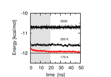
Figure 1: Timeseries of the potential energy of the SWM4-NDP water model for three different temperatures. Below 190 K relaxation times become very long as depicted by the 170 K trajectory (red) and the gray region.

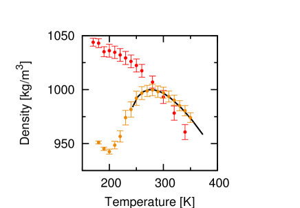
Figure 2: The density curve at 1 atm. Data for SWM4-NDP, TIP4P/2005 and experiments Kell (1975) are shown in red, orange and black, respectively.

Molecular dynamics simulations of the Drude-based polarizable water model SWM4-NDP were performed at several temperatures spanning from 170 K to 340 K. Running simulations for temperatures as low as 180 K, Kiss and Baranyai Kiss and Baranyai (2012) recently showed that this model presents no density maximum. Independently from them we were also looking at the same problem. One important difference in our work is that simulations were run for much longer times: 50 ns per trajectory opposed to 5 ns in their case.

Our results strongly indicate that long runs of several ns are needed to characterize SWM4-NDP in the deeply supercooled regime. This becomes clear when looking at the time series of the potential energy. In Fig. 1A traces for different temperatures from 250 K to 170 K are shown. It was found that for temperatures lower than 200 K the relaxation time of the system dramatically slows down. The red line corresponding to 170 K shows that the system required at least 20 ns to equilibrate (gray region). This is a much longer time than the simulation length used in Ref. Kiss and Baranyai (2012).

With the longer trajectories at hand, the density curve did present a maximum at around 200 K (red points in Fig. 2), a value that is similar to what was found for TIP3P (182 K Vega and Abascal (2005)). However, this maximum is not a global one as in experiments (black line) or in other classical models like TIP4P/2005 (orange points). In fact, at lower temperatures (T$<$190 K) density grows again, making the density peak difficult to emerge from the statistical error, especially when using short trajectories. An increase of the density passed the density maximum is a feature of several water models. For example, this happens as well for TIP4P/2005 below 200 K (Fig. 2). What makes SWM4-NDP peculiar is the fact that the value of the density in this regime becomes even higher than the density maximum, making the latter a relative maximum (not an absolute one).

III.2 Hydrogen-bond propensities and temperature-shifts

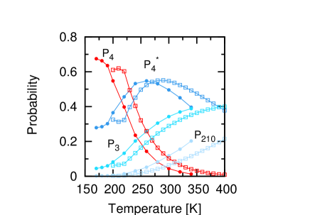
Figure 3: Hydrogen bond propensities including the second solvation shell. $P_{4}$, $P^{*}_{4}$, $P_{3}$ and $P_{210}$ are shown in red, dark blue, blue and light blue, respectively (see Methods for details). Data for SWM4-NDP and TIP4P/2005 are shown as filled circles and empty squares, respectively.

Complementary information was obtained by investigating hydrogen-bond propensities. As done recently for seven classical water models Shevchuk et al. (2012) we calculated the probability to form fully coordinated hydrogen-bond configurations up to the second shell ($P_{4}$, red in Fig. 3; see Methods) as well as fully coordinated first shells with a disordered second shell ($P^{*}_{4}$, dark blue), three coordinated ($P_{3}$, blue) and less ($P_{210}$, light blue) first solvation shells. Results for the SWM4-NDP and TIP4P/2005 for comparison are shown in Fig. 3 as filled circles and empty squares, respectively. Contrary to the density analysis, hydrogen-bond propensities between the two models look much more similar (e.g. TIP3P showed a much more drastic temperature shift of 60 K Shevchuk et al. (2012)). The two sets of curves would nicely overlap if a shift of approximately 20 K is applied to the data. This observation suggests that while spatial rearrangement responsible for the density is dramatically different between the two models (and when compared to experiments), hydrogen-bond connectivity is similar. Such a discrepancy was already observed when comparing three-sites with four-sites models where a 10 K difference between temperature shifts estimated from hydrogen bonds or the position of the density maximum was observed Shevchuk et al. (2012). But in this case the discrepancy is much larger being the temperature shifts respectively of 20 K and 80 K, i.e. a 40 K difference between the two approaches.

III.3 Tetrahedral order parameter

Figure 4: Tetrahedral order parameter. (Top) Average value of the parameter as a function of temperature. (Bottom) parameter distribution at 300 K. Data for SWM4-NDP and TIP4P/2005 are shown in red and orange, respectively.

Temperature shifts were observed as well when comparing the two models on the base of the average value of the tetrahedral order parameter $Q$ (see Methods). The top panel of Fig. 4 shows this quantity as a function of temperature for both SWM4-NDP (red line) and TIP4P/2005 (orange). As for the case of the hydrogen-bond propensities $P_{i}^{(*)}$, the two models do not differ very much. At ambient conditions the temperature-shift is of about 30 K, a number that is in line with what observed for the hydrogen-bond propensities (Fig. 3). For the sake of comparison the distribution of $Q$ at 300 K for the two models is shown at the bottom of Fig. 4. As it could have been expected from the behavior of the average value of the order parameter, TIP4P/2005 has a slightly larger fraction of molecules in a tetrahedral configuration but the overall shape of the distribution is similar for the two cases. This is even clearer when presenting the data for TIP4P/2005 at a 30 K higher temperature (gray curve): now the distribution for SWM4-NDP and the temperature-shifted TIP4P/2005 nicely overlap on top of each other with good approximation.

IV Discussion

In the present work, we performed extensive molecular dynamics simulations of the Drude-based polarizable water model SWM4-NDP as a function of temperature. Contrary to what was reported in a recent paper Kiss and Baranyai (2012), it was found that the model do present a density maximum which was found to be around 200 K. The density curve was not easy to calculate because of the intrinsic slowing down of the system for temperatures lower than 200 K that hindered the detection of the maximum. To overcome this problem simulation runs of 50 ns each were performed, finding that at temperatures below 200 K the system required at least 20 ns to have the potential energy relaxing to a stationary average value without drifts.

However, the density maximum we found is not as pronounced as other classical water models or in experiments. This was somewhat unexpected. As system temperature was lowered below 190 K, the density started to increase again. This is only in principle similar to what was observed for other models, like for example TIP4P/2005. In fact, in the present case the density value increased to a value that is larger than the density maximum, making the latter a relative maximum instead of an absolute one. The raising of the density at a such low temperature is probably due to some sort of frustration into the system leading to glassy behavior. This idea would also explain the dramatic slowing down of the relaxation kinetics of the model below 200 K.

In comparison to other classical models, SWM4-NDP performed very poorly in reproducing the density curve. This is somewhat disappointing given the success of other models in this respect, especially the reparametrized versions of the four-site model, TIP4P/2005 Abascal and Vega (2005) and TIP4P-Ew Horn et al. (2004) as well as the newly presented iAMOEBA polarizable model Wang et al. (2013).

Despite the position of the density maximum of SWM4-NDP is shifted by roughly 80 K, the behavior of the hydrogen-bond propensities and tetrahedrality are very well in line to what the best models in the field predict. This behavior differs from what we found in the past for other non-polarizable water models, i.e. that a temperature-shift in the density maximum corresponds to a similar shift in the hydrogen-bond propensities. The presence of polarizability instead completely decouples these two aspects, giving in principle a wider space to match experimental data, at least in principle.

In conclusion, our work shed some further light on the behavior of the SWM4-NDP polarizable model in temperature space. The great advantage of this model with respect to other approaches is the easy integration in all modern force-fields for biomolecular simulations. However, our results suggest that to make this model fully effective, a new parametrization able to reproduce the density curve and other quantities in temperature space is required.

References

- Vega and Abascal (2011) C. Vega and J. L. F. Abascal, Phys. Chem. Chem. Phys. 13, 19663 (2011).
- Matsumoto et al. (2002) M. Matsumoto, S. Saito, and I. Ohmine, Nature 416, 409 (2002).
- Moore and Molinero (2011) E. B. Moore and V. Molinero, Nature 479, 506 (2011).
- Vega and Abascal (2005) C. Vega and J. L. F. Abascal, J. Chem. Phys. 123, 144504 (2005).
- Abascal et al. (2005) J. L. F. Abascal, E. Sanz, R. G. Fernández, and C. Vega, J. Chem. Phys. 122, 234511 (2005).
- Mahoney and Jorgensen (2000) M. W. Mahoney and W. L. Jorgensen, J. Chem. Phys. 112, 8910 (2000).
- Horn et al. (2004) H. W. Horn, W. C. Swope, J. W. Pitera, J. D. Madura, T. J. Dick, G. L. Hura, and T. Head-Gordon, J. Chem. Phys. 120, 9665 (2004).
- Abascal and Vega (2005) J. L. F. Abascal and C. Vega, J. Chem. Phys. 123, 234505 (2005).
- Mark and Nilsson (2001) P. Mark and L. Nilsson, J. Phys. Chem. A 105, 9954 (2001).
- Vega et al. (2005) C. Vega, E. Sanz, and J. L. F. Abascal, J. Chem. Phys. 122, 114507+ (2005).
- Lamoureux and Roux (2006) G. Lamoureux and B. Roux, J. Phys. Chem. B 110, 3308 (2006).
- Brooks et al. (2009) B. R. Brooks, C. L. Brooks, A. D. Mackerell, L. Nilsson, R. J. Petrella, B. Roux, Y. Won, G. Archontis, C. Bartels, S. Boresch, et al., J. Comput. Chem. 30, 1545 (2009).
- Baranyai and Kiss (2010) A. Baranyai and P. T. Kiss, J. Chem. Phys. 133, 144109 (2010).
- Ren and Ponder (2003) P. Ren and J. W. Ponder, J. Phys. Chem B 107, 5933 (2003).
- Lamoureux et al. (2003) G. Lamoureux, M. A. D., and B. Roux, J. Chem. Phys. 119, 5185 (2003).
- Halgren (1992) T. A. Halgren, J. Am. Chem. Soc. 114, 7827 (1992).
- Wang et al. (2013) L.-P. Wang, T. L. Head-Gordon, J. W. Ponder, P. Ren, J. D. Chodera, P. K. Eastman, T. J. Martínez, and V. S. Pande, J. Phys. Chem. B 117, 9956 (2013).
- van Maaren and van der Spoel (2001) P. J. van Maaren and D. van der Spoel, J. Phys. Chem. B 105, 2618 (2001).
- Lamoureux et al. (2006) G. Lamoureux, E. Harder, I. V. Vorobyov, B. Roux, and A. D. MacKerell Jr, Chem. Phys. Lett. 418, 245 (2006).
- Stukan et al. (2013) M. R. Stukan, A. Asmadi, and W. Abdallah, J. Mol. Liq. 180, 65 (2013).
- Bruneval et al. (2007) F. Bruneval, D. Donadio, and M. Parrinello, J. Phys. Chem. B 111, 12219 (2007).
- Nelson et al. (1996) M. T. Nelson, W. Humphrey, A. Gursoy, A. Dalke, L. V. Kalé, R. D. Skeel, and K. Schulten, Int. J. High Perform. C. 10, 251 (1996).
- Jiang et al. (2010) W. Jiang, D. J. Hardy, J. C. Phillips, A. D. MacKerell Jr, K. Schulten, and B. Roux, J. Phys. Chem. Lett. 2, 87 (2010).
- Van Der Spoel et al. (2005) D. Van Der Spoel, E. Lindahl, B. Hess, G. Groenhof, A. E. Mark, and H. J. C. Berendsen, J. Comput. Chem. 26, 1701 (2005).
- Berendsen et al. (1984) H. J. C. Berendsen, J. P. M. Postma, W. F. van Gunsteren, A. DiNola, and J. R. Haak, J. Chem. Phys. 81, 3684 (1984).
- Bussi et al. (2007) G. Bussi, D. Donadio, and M. Parrinello, J. Chem. Phys. 126, 014101 (2007).
- Darden et al. (1993) T. Darden, D. York, and L. Pedersen, J. Chem. Phys. 98, 10089 (1993).
- Luzar and Chandler (1996) A. Luzar and D. Chandler, Phys. Rev. Lett. 76, 928 (1996).
- Shevchuk et al. (2012) R. Shevchuk, D. Prada-Gracia, and F. Rao, J. of Phys. Chem. B 116, 7538 (2012).
- Errington and Debenedetti (2001) J. R. Errington and P. G. Debenedetti, Nature 409, 318 (2001).
- Kell (1975) G. S. Kell, J. Chem. Eng. Data 20, 97 (1975).
- Kiss and Baranyai (2012) P. T. Kiss and A. Baranyai, J. Chem. Phys. 137, 084506 (2012).