Empirical likelihood on the full parameter space

Abstract

We extend the empirical likelihood of Owen [Ann. Statist. 18 (1990) 90–120] by partitioning its domain into the collection of its contours and mapping the contours through a continuous sequence of similarity transformations onto the full parameter space. The resulting extended empirical likelihood is a natural generalization of the original empirical likelihood to the full parameter space; it has the same asymptotic properties and identically shaped contours as the original empirical likelihood. It can also attain the second order accuracy of the Bartlett corrected empirical likelihood of DiCiccio, Hall and Romano [Ann. Statist. 19 (1991) 1053–1061]. A simple first order extended empirical likelihood is found to be substantially more accurate than the original empirical likelihood. It is also more accurate than available second order empirical likelihood methods in most small sample situations and competitive in accuracy in large sample situations. Importantly, in many one-dimensional applications this first order extended empirical likelihood is accurate for sample sizes as small as ten, making it a practical and reliable choice for small sample empirical likelihood inference.

and

t1Supported by a research grant from the National Science and Engineering Research Council of Canada.

1 Introduction

Since the seminal work of Owen (1988, 1990), there have been many advances in empirical likelihood method that have brought applications of the method to virtually every area of statistical research. It has been widely observed [e.g., Hall and La Scala (1990), Qin and Lawless (1994), Corcoran, Davison and Spady (1995), Owen (2001), Liu and Chen (2010)] that empirical likelihood ratio confidence regions can have poor accuracy, especially in small sample and multidimensional situations. In particular, there is a persistent undercoverage problem in that coverage probabilities of empirical likelihood ratio confidence regions tend to be lower than the nominal levels. In this paper, we tackle a fundamental problem underlying the poor accuracy and undercoverage, that is, the empirical likelihood is defined on only a part of the parameter space. We call this the mismatch problem between the domain of the empirical likelihood and the parameter space. We solve this problem through a geometric approach that expands the domain to the full parameter space. Our solution brings about substantial improvements in accuracy of the empirical likelihood inference and is particularly useful for small sample and multidimensional situations.

To see the mismatch problem, consider the example of empirical likelihood for the mean based on $n$ observations $X_{1},\ldots,X_{n}$ of a random vector $X\in\mathbb{R}^{d}$. The underlying parameter space $\Theta$ is $\mathbb{R}^{d}$ itself. But for a given $\theta\in\mathbb{R}^{d}$, when the convex hull of the $(X_{i}-\theta)$ does not contain $0$, the empirical likelihood $L(\theta)$, the empirical likelihood ratio $R(\theta)=n^{n}L(\theta)$ and the empirical log-likelihood ratio $l(\theta)=-2\log R(\theta)$ are all undefined. When this occurs, an established convention assigns $L(\theta)=0$, and technically $L(\theta)$, $R(\theta)$ and $l(\theta)$ are now defined over the full parameter space. Nevertheless, to highlight the difference between the natural domain of the empirical likelihood and the parameter space, we define the common domain of $L(\theta)$, $R(\theta)$ and $l(\theta)$ as

$$\Theta_{n}=\bigl{\{}\theta\dvtx\theta\in\Theta\mbox{ and }l(\theta)<+\infty\bigr{\}}.$$ (1)

With this definition, the mismatch can now be expressed as $\Theta_{n}\subset\Theta$. For the mean, $\Theta_{n}$ is the interior of the convex hull of the $X_{i}$, which is indeed a proper subset of $\Theta=\mathbb{R}^{d}$. The mismatch $\Theta_{n}\subset\Theta$ holds for empirical likelihoods in general as the basic formulation common to all empirical likelihoods has a convex hull constraint on the origin, such as the one for the mean above, which may be violated by some $\theta$ values in the parameter space $\Theta$.

The convex hull constraint violation underlying the mismatch is well known in the empirical likelihood literature. It was first noted in Owen (1990) for the case of the mean. See also Owen (2001). To assess its impact on coverage probabilities of empirical likelihood ratio confidence regions, Tsao (2004) investigated bounds on coverage probabilities resulting from the convex hull constraint. To bypass this constraint, Bartolucci (2007) introduced a penalized empirical likelihood (PEL) for the mean which removes the convex hull constraint in the formulation of the original empirical likelihood (OEL) of Owen (1990, 2001) and replaces it with a penalizing term based on the Mahalanobis distance. For parameters defined by general estimating equations, Chen, Variyath and Abraham (2008) introduced an adjusted empirical likelihood (AEL) which retains the formulation of the OEL but adds a pseudo-observation to the sample. The AEL is just the OEL defined on the augmented sample. But due to the clever construction of the pseudo-observation, the convex hull constraint will never be violated by the AEL. Emerson and Owen (2009) showed that the AEL statistic has a boundedness problem which may lead to trivial 100% confidence regions. They proposed an extension of the AEL involving adding two pseudo-observations to the sample to address the boundedness problem. Chen and Huang (2013) also addressed the boundedness problem by modifying the adjustment factor in the pseudo-observation. Liu and Chen (2010) proved a surprising result that under a certain level of adjustment, the AEL confidence region achieves the second order accuracy of the Bartlett corrected empirical likelihood (BEL) region by DiCiccio, Hall and Romano (1991). Recently, Lahiri and Mukhopadhyay (2012) showed that under certain dependence structures, a modified PEL for the mean works in the extremely difficult case of large dimension and small sample size. The PEL and the AEL are both defined on $\mathbb{R}^{d}$, and are thus free from the mismatch problem.

In this paper, we propose a new extended empirical likelihood (EEL) that is also free from the mismatch problem. We derive this EEL through the domain expansion method of Tsao (2013) which expands the domain of the OEL but retains its important geometric characteristics. This EEL makes effective use of the dimension information in the data and can attain the second order accuracy of the BEL. The most important aspect of this EEL, however, is that there is an easy-to-use first order version which is substantially more accurate than the OEL. This first order EEL is also more accurate than available second order empirical likelihood methods in most small sample and multidimensional applications and is comparable in accuracy to the latter when the sample size is large. The focus of the present paper is on the construction of EEL for the mean through which we introduce the basic idea of and important tools for expanding the OLE domain to the full parameter space. Under certain conditions, EEL for other parameters may also be constructed but this will be discussed elsewhere.

For brevity, we will use “OEL $l(\theta)$” and “EEL $l^{*}(\theta)$” to refer to the original and extended empirical log-likelihood ratios for the mean, respectively. Throughout this paper, we assume that the parameter space $\Theta$ is $\mathbb{R}^{d}$. The case where $\Theta$ is a known subset of $\mathbb{R}^{d}$ can be handled by finding EEL $l^{*}(\theta)$ defined on $\mathbb{R}^{d}$ first and then, for $\theta\notin\Theta$ only, redefine it as $l^{*}(\theta)=+\infty$.

2 Preliminaries

We review several key results and assumptions for developing the EEL defined on the full parameter space.

2.1 Empirical likelihood for the mean

Let $X\in\mathbb{R}^{d}$ be a random vector with mean $\theta_{0}$ and covariance matrix $\Sigma_{0}$. Two assumptions we will need are: [$(A_{2})$]

$\Sigma_{0}$ is a finite covariance matrix with full rank $d$; and

$\lim\sup_{\|t\|\rightarrow\infty}|E[\exp\{it^{T}X\}]|<1$ and $E\|X\|^{15}<+\infty$. These are also assumptions under which the OEL for the mean is Bartlett correctable [DiCiccio, Hall and Romano (1988), Chen and Cui (2007)].

Let $X_{1},\ldots,X_{n}$ be independent copies of $X$ where $n>d$. Let $\Theta_{n}$ be the collection of points in the interior of the convex hull of the $X_{i}$. For a $\theta\in\mathbb{R}^{d}$, Owen (1990) defined the empirical likelihood ratio $R(\theta)$ as

$$R(\theta)=\sup\Biggl{\{}\prod_{i=1}^{n}nw_{i}\Big{|}\sum_{i=1}^{n}w_{i}(X_{i}-\theta)=0,w_{i}\geq 0,\sum_{i=1}^{n}w_{i}=1\Biggr{\}}.$$ (2)

It may be verified that $0<R(\theta)\leq 1$ iff $\theta\in\Theta_{n}$. Also, $R(\theta)=0$ if $\theta\notin\Theta_{n}$. Hence, the domain of the OEL $l(\theta)=-2\log R(\theta)$ is $\Theta_{n}$. For a $\theta\in\Theta_{n}$, the method of Lagrange multipliers may be used to show that

$$l(\theta)=2\sum^{n}_{i=1}\log\bigl{\{}1+\lambda^{T}(X_{i}-\theta)\bigr{\}},$$ (3)

where the multiplier $\lambda=\lambda(\theta)\in\mathbb{R}^{d}$ satisfies

$$\sum_{i=1}^{n}\frac{X_{i}-\theta}{1+\lambda^{T}(X_{i}-\theta)}=0.$$ (4)

Under assumption ($A_{1}$), Owen (1990) showed that OEL $l(\theta)$ satisfies

$$l(\theta_{0})\stackrel{{\scriptstyle\mathcal{D}}}{{\longrightarrow}}\chi^{2}_{d}\qquad\mbox{as $n\rightarrow+\infty$}.$$ (5)

For an $\alpha\in(0,1)$, let $c$ be the ($1-\alpha$)th quantile of the $\chi^{2}_{d}$ distribution. Then, the $100(1-\alpha)\%$ OEL confidence region for $\theta_{0}$ is given by

$${\mathcal{C}}_{1-\alpha}=\bigl{\{}\theta\dvtx\theta\in\Theta_{n}\mbox{ and }l(\theta)\leq c\bigr{\}}.$$ (6)

Under assumptions ($A_{1}$) and ($A_{2}$), DiCiccio, Hall and Romano (1988, 1991) showed that the coverage error of ${\mathcal{C}}_{1-\alpha}$ is $O(n^{-1})$, that is,

$$P(\theta_{0}\in{\mathcal{C}}_{1-\alpha})=P\bigl{(}l(\theta_{0})\leq c\bigr{)}=P\bigl{(}\chi^{2}_{d}\leq c\bigr{)}+O\bigl{(}n^{-1}\bigr{)}.$$ (7)

More importantly, they showed that the empirical likelihood is Bartlett correctable. To give a brief account of this surprising result, let

$${\mathcal{C}}_{1-\alpha}^{\prime}=\bigl{\{}\theta\dvtx l(\theta)\bigl{(}1-bn^{-1}\bigr{)}\leq c\bigr{\}}$$ (8)

be the Bartlett corrected empirical likelihood ratio confidence region where $b$ is the Bartlett correction constant and $(1-bn^{-1})$ is the Bartlett correction factor, DiCiccio, Hall and Romano (1988, 1991) showed that ${\mathcal{C}}_{1-\alpha}^{\prime}$ has a coverage error of only $O(n^{-2})$, that is,

$$P\bigl{(}\theta_{0}\in{\mathcal{C}}_{1-\alpha}^{\prime}\bigr{)}=P\bigl{[}l(\theta_{0})\bigl{(}1-bn^{-1}\bigr{)}\leq c\bigr{]}=P\bigl{(}\chi^{2}_{d}\leq c\bigr{)}+O\bigl{(}n^{-2}\bigr{)}.$$ (9)

In practice, the Bartlett correction constant $b$ cannot be determined since it depends on the moments of $X$ which are not available in the nonparametric setting of the empirical likelihood. However, replacing the Bartlett correction factor in (9) with $[1-bn^{-1}+O_{p}(n^{-3/2})]$ does not affect the $O(n^{-2})$ term in its right-hand side, that is,

$$P\bigl{\{}l(\theta_{0})\bigl{[}1-bn^{-1}+O_{p}\bigl{(}n^{-3/2}\bigr{)}\bigr{]}\leq c\bigr{\}}=P\bigl{(}\chi^{2}_{d}\leq c\bigr{)}+O\bigl{(}n^{-2}\bigr{)}.$$ (10)

This allows us to replace $b$ in (8) and (9) with a $\sqrt{n}$-consistent estimate $\hat{b}$ without invalidating (9). See DiCiccio, Hall and Romano (1991) and Hall and La Scala (1990) for detailed discussions on Bartlett correction.

2.2 Extended empirical likelihood

The OEL confidence region ${\mathcal{C}}_{1-\alpha}$ in (6) is confined to the OEL domain $\Theta_{n}$. This is a main cause of the undercoverage problem associated with ${\mathcal{C}}_{1-\alpha}$ [Tsao (2004)]. To alleviate the problem, Tsao (2013) proposed to expand $\Theta_{n}$ which will lead to larger EL confidence regions. Let $h_{n}\dvtx\mathbb{R}^{d}\rightarrow\mathbb{R}^{d}$ be a bijective mapping and define a new empirical log-likelihood ratio $l^{*}(\theta)$ through the OEL $l(\theta)$ as follows:

$$l^{*}(\theta)=l\bigl{(}h^{-1}_{n}(\theta)\bigr{)}\qquad\mbox{for $\theta\in\mathbb{R}^{d}$}.$$ (11)

Then the domain for the new empirical log-likelihood ratio is $\Theta_{n}^{*}=h_{n}(\Theta_{n})$. Here, $h_{n}$ plays the role of reassigning or extending the OEL values of points in $\Theta_{n}$ to points in $\Theta_{n}^{*}$. Because of this, Tsao (2013) named $l^{*}(\theta)$ the extended empirical log-likelihood ratio or simply EEL. In particular, Tsao (2013) used the following $\tilde{\theta}$-centred similarity mapping $h_{n}^{*}\dvtx\mathbb{R}^{d}\rightarrow\mathbb{R}^{d}$

$$h_{n}^{*}(\theta)=\tilde{\theta}+\gamma_{n}(\theta-\tilde{\theta}),$$ (12)

where $\tilde{\theta}$ is the sample mean and $\gamma_{n}\in\mathbb{R}^{1}$ is a constant (which we will refer to as the expansion factor) satisfying $\gamma_{n}\geq 0$ and $\gamma_{n}\rightarrow 1$ as $n\rightarrow+\infty$. If we choose $\gamma_{n}>1$, then $\Theta_{n}\subset\Theta^{*}_{n}\subset\mathbb{R}^{d}$, and $\Theta^{*}_{n}$ alleviates the mismatch problem of $\Theta_{n}$. The EEL confidence region for $\theta_{0}$ is given by

$${\mathcal{C}}_{1-\alpha}^{*}=\bigl{\{}\theta\dvtx\theta\in\Theta^{*}_{n}\mbox{ and }l^{*}(\theta)\leq c\bigr{\}}.$$ (13)

The advantages of the EEL based on $h_{n}^{*}$ in (12) are: (1) the EEL confidence regions are similarly transformed OEL confidence regions, as such they retain the natural centre and shape of the OEL confidence regions, (2) the EEL can be applied to empirical likelihood inference for a wide range of parameters, and (3) with a properly selected constant $\gamma_{n}$, EEL confidence regions can achieve the second order accuracy of $O(n^{-2})$.

Nevertheless, the EEL based on $h_{n}^{*}$ is only a partial solution to the mismatch problem because the domain of this EEL $\Theta^{*}_{n}$ is also a proper subset of $\mathbb{R}^{d}$. A second order version of this EEL has been found to have good accuracy in one- and two-dimensional problems. But it also tends to undercover and no accurate first order version of this EEL is available. These motivated us to consider an EEL defined on the full parameter space.

3 Extended empirical likelihood on the full parameter space

Consider a bijective mapping from the OEL domain to the parameter space, $h_{n}\dvtx\Theta_{n}\rightarrow\Theta=\mathbb{R}^{d}$. Under such a mapping, the EEL $l^{*}(\theta)$ given by (11) is well defined throughout $\mathbb{R}^{d}$ and is thus free from the mismatch problem. In this section, we first construct such a mapping using $h_{n}^{*}$ in (12). We call it the composite similarity mapping and denote it by $h^{C}_{n}\dvtx\Theta_{n}\rightarrow\mathbb{R}^{d}$. We then study the asymptotic properties of the EEL $l^{*}(\theta)$ based on $h^{C}_{n}$.

3.1 The composite similarity mapping

The simple similarity mapping $h_{n}^{*}$ in (12) maps OEL domain $\Theta_{n}$ onto a similar but bounded region in $\mathbb{R}^{d}$. If we think of $\Theta_{n}$ as a region consisting of distinct and nested contours of the OEL, then $h_{n}^{*}$ expands all contours with the same constant expansion factor $\gamma_{n}$. In order to map $\Theta_{n}$ onto the full $\mathbb{R}^{d}$, we need to expand contours on the outside more and more so that the images of the contours will fill up the entire $\mathbb{R}^{d}$. To achieve this, consider level-$\tau$ contour of the OEL $l(\theta)$,

$$c(\tau)=\bigl{\{}\theta\dvtx\theta\in\Theta_{n}\mbox{ and }l(\theta)=\tau\bigr{\}},$$ (14)

where $\tau\geq 0$. The contours form a partition of the OEL domain,

$$\Theta_{n}=\bigcup_{\tau\in[0,+\infty)}c(\tau).$$ (15)

In light of (15), the centre of $\Theta_{n}$ is $c(0)=\{\tilde{\theta}\}$ and the outwardness of a $c(\tau)$ with respect to the centre is indexed by $\tau$; the larger the $\tau$ value, the more outward $c(\tau)$ is. If we allow the expansion factor $\gamma_{n}$ to be a continuous monotone increasing function of $\tau$ and allow $\gamma_{n}$ to go to infinity when $\tau$ goes to infinity, then (such a variation of) $h_{n}^{*}$ will map $\Theta_{n}$ onto $\mathbb{R}^{d}$. Hence, we define the composite similarity mapping $h^{C}_{n}\dvtx\Theta_{n}\rightarrow\mathbb{R}^{d}$ as follows:

$$h_{n}^{C}(\theta)=\tilde{\theta}+\gamma\bigl{(}n,l(\theta)\bigr{)}(\theta-\tilde{\theta})\qquad\mbox{for $\theta\in\Theta_{n}$},$$ (16)

where $\gamma(n,l(\theta))$ is given by

$$\gamma\bigl{(}n,l(\theta)\bigr{)}=1+\frac{l(\theta)}{2n}.$$ (17)

Function $\gamma(n,l(\theta))$ is the new expansion factor which depends continuously on $\theta$ through the value of $l(\theta)$ or $\tau=l(\theta)$. For convenience, we will emphasis the dependence of $\gamma(n,l(\theta))$ on $l(\theta)$ instead of $\theta$ or $\tau$. This new expansion factor has the two desired properties discussed above:

for a fixed $$n l(\theta_{1})<l(\theta_{2}) \gamma\bigl{(}n,l(\theta_{2})\bigr{)}<\gamma\bigl{(}n,l(\theta_{2})\bigr{)}$$, if , then ; and (19)

for a fixed $$n \gamma\bigl{(}n,l(\theta)\bigr{)}\rightarrow+\infty l(\theta)\rightarrow+\infty$$, as .

The inclusion of the denominator $2n$ in (17) ensures that the expansion factor converges to 1, reflecting the fact that there is no need for domain expansion for large sample sizes. Also, the constant $2$ in the denominator provides extra adjustment to the speed of expansion and may be replaced with other positive constants (see Figure 1). We choose to use 2 here as the corresponding $\gamma(n,l(\theta))$ in (17) is asymptotically equivalent to a likelihood based expansion factor $\gamma(n,L(\theta))=L(\theta)^{-1/n}$ which we had first considered and was found to give accurate numerical results. The definition of $\gamma(n,l(\theta))$ in (17) uses $l(\theta)$ instead of $L(\theta)$ because of convenience for theoretical investigations. A more general form of $\gamma(n,l(\theta))$ will be considered later.

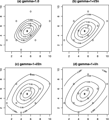
Figure 1: (a) Contours of the OEL $l(\theta)$ (for which the expansion factor is 1.0); (b) contours of the EEL $l^{*}(\theta)$ with expansion factor $\gamma(11,l(\theta))=1+l(\theta)/3n$; (c) contours of the EEL $l^{*}(\theta)$ with $\gamma(11,l(\theta))=1+l(\theta)/2n$; (d) contours of the EEL $l^{*}(\theta)$ with $\gamma(11,l(\theta))=1+l(\theta)/n$. All four plots are based on the same random sample of 11 points shown in small circles. The star in the middle is the sample mean. The expansion factor increases as we go from plot (b) to plot (d), and correspondingly the EEL contours also become bigger in scale from plot (b) to (d). But the centre and shapes of contours are the same in all plots.

Theorem 3.1 below summarizes the key properties of the composite similarity mapping $h_{n}^{C}$. Its proof and that of subsequent theorems and lemmas may all be found in the Appendix.

Theorem 3.1

Under assumption ($A_{1}$), the composite similarity mapping $h^{C}_{n}\dvtx\Theta_{n}\rightarrow\mathbb{R}^{d}$ defined by (16) and (17) satisfies:

it has a unique fixed point at the mean $\tilde{\theta}$;

it is a similarity mapping for each individual $c(\tau)$; and

it is a bijective mapping from $\Theta_{n}$ to $\mathbb{R}^{d}$.

Because of (ii) above, we call $h_{n}^{C}$ the composite similarity mapping as it may be viewed as a continuous sequence of simple similarity mappings from $\mathbb{R}^{d}$ to $\mathbb{R}^{d}$ indexed by $\tau=l(\theta)\in[0,+\infty)$. The “$\tau$th” mapping from this sequence has expansion factor $\gamma(n,l(\theta))=\gamma(n,\tau)$. It is just the simple similarity mapping $h_{n}^{*}$ in (12) with $\gamma_{n}=\gamma(n,\tau)$, and is used exclusively to map the “$\tau$th” OEL contour $c(\tau)$. The latter has been implicitly built into $h_{n}^{C}$ since for all $\theta\in c(\tau)$, $l(\theta)=\tau$ which implies the corresponding expansion factor of $h_{n}^{C}$ is the constant $\gamma(n,\tau)$ that defines the “$\tau$th” mapping.

It should be noted that $h_{n}^{C}$ is not a similarity mapping from $\mathbb{R}^{d}$ to $\mathbb{R}^{d}$ itself due to the dependence of the expansion factor $\gamma(n,l(\theta))$ on $\theta$ and its domain $\Theta_{n}$ which is only a bounded subset of $\mathbb{R}^{d}$.

3.2 The extended empirical likelihood under the composite similarity mapping

By Theorem 3.1, $h_{n}^{C}\dvtx\Theta_{n}\rightarrow\mathbb{R}^{d}$ is bijective. Hence, it has an inverse which we denote by $h_{n}^{-C}\dvtx\mathbb{R}^{d}\rightarrow\Theta_{n}$. The EEL $l^{*}(\theta)$ under $h_{n}^{C}$ is

$$l^{*}(\theta)=l\bigl{(}h_{n}^{-C}(\theta)\bigr{)}\qquad\mbox{for $\theta\in\mathbb{R}^{d}$},$$

which is defined throughout $\mathbb{R}^{d}$. The contours of $l^{*}(\theta)$ are larger in scale but have the same centre and identical shape as that of OEL $l(\theta)$. Figure 1 compares their contours with a sample of 11 two-dimensional observations. It shows that geometrically, mapping $h_{n}^{C}$ is anchored at the sample mean $\tilde{\theta}$ as it is the fixed point of $h_{n}^{C}$ that is not moved. From this anchoring point, the mapping pushes out/expands each OEL contour $c(\tau)$ proportionally in all directions at an expansion factor of $\gamma(n,\tau)$ to form an EEL contour. The boundary points of $\Theta_{n}$ are all pushed out to the infinity.

In the following, we will use $\theta^{\prime}$ to denote the image of a $\theta\in\mathbb{R}^{d}$ under the inverse transformation $h_{n}^{-C}$, that is, $h_{n}^{-C}(\theta)=\theta^{\prime}\in\Theta_{n}$. Of particular interest is the image of the unknown true mean $\theta_{0}$,

$$h_{n}^{-C}(\theta_{0})=\theta_{0}^{\prime}.$$ (20)

Because the inverse transformation $h_{n}^{-C}$ does not have an analytic expression, that for $\theta^{\prime}_{0}$ is also not available. Nevertheless, Lemma 3.2 gives an asymptotic assessment on its distance to $\theta_{0}$. The proof of Lemma 3.2 will need Lemma 3.1 below which shows that inside $\Theta_{n}$, the OEL $l(\theta)$ is a “monotone increasing” function along each ray originating from the mean $\tilde{\theta}$.

Lemma 3.1

Under assumption ($A_{1}$), for a fixed point $\theta\in\Theta_{n}$ and any value $\alpha\in[0,1]$ the OEL $l(\theta)$ satisfies

$$l\bigl{(}\tilde{\theta}+\alpha(\theta-\tilde{\theta})\bigr{)}\leq l(\theta).$$

Denote by $[\tilde{\theta},\theta_{0}]$ the line segment connecting $\tilde{\theta}$ and $\theta_{0}$. Lemma 3.2 below shows that $\theta_{0}^{\prime}$ is on $[\tilde{\theta},\theta_{0}]$ and is asymptotically very close to $\theta_{0}$.

Lemma 3.2

Under assumption ($A_{1}$), point $\theta_{0}^{\prime}$ defined by equation (20) satisfies (i) $\theta_{0}^{\prime}\in[\tilde{\theta},\theta_{0}]$ and (ii) $\theta^{\prime}_{0}-\theta_{0}=O_{p}(n^{-3/2})$.

Using $\theta_{0}^{\prime}$, the EEL $l^{*}(\theta_{0})$ can now be expressed as

$$l^{*}(\theta_{0})=l\bigl{(}h_{n}^{-C}(\theta_{0})\bigr{)}=l\bigl{(}\theta^{\prime}_{0}\bigr{)}=l\bigl{(}\theta_{0}+\bigl{(}\theta_{0}^{\prime}-\theta_{0}\bigr{)}\bigr{)}.$$ (21)

The following theorem gives the asymptotic distribution of $l^{*}(\theta_{0})$:

Theorem 3.2

Under assumption ($A_{1}$) and with the composite similarity mapping $h_{n}^{C}$ defined by (16) and (17), the EEL $l^{*}(\theta)$ satisfies

$$l^{*}(\theta_{0})\stackrel{{\scriptstyle\mathcal{D}}}{{\longrightarrow}}\chi^{2}_{d}\qquad\mbox{as $n\rightarrow+\infty$}.$$ (22)

The proof of Theorem 3.2 is based on the observation that $\|\theta_{0}^{\prime}-\theta_{0}\|$ is asymptotically very small. This and (21) imply that $l^{*}(\theta_{0})=l(\theta_{0})+o_{p}(1)$. This proof demonstrates an advantage of the EEL: it has the simple relationship with the OLE shown in (21) through which we make use of known asymptotic properties of the OEL to study the EEL. Our derivation of a second order EEL below further explores this advantage.

3.3 Second order extended empirical likelihood

It may be verified that Theorems 3.1 and 3.2 also hold under any composite similarity mapping defined by (16) and the following general form of the expansion factor,

$$\gamma\bigl{(}n,l(\theta)\bigr{)}=1+\frac{\kappa[l(\theta)]^{\delta(n)}}{n^{m}},$$ (23)

where $\kappa$ and $m$ are both positive constants and $\delta(n)$ is a bounded function of $n$ satisfying $\varepsilon_{n}<\delta(n)\leq a$ for some constants $a>\varepsilon_{n}>0$. The availability of a whole family of $\gamma(n,l(\theta))$ functions for the construction of the EEL provides an opportunity to optimize our choice of this function to achieve the second order accuracy. Theorem 3.3 below gives the optimal choice.

Theorem 3.3

Assume $(A_{1})$ and $(A_{2})$ hold and denote by $l^{*}_{s}(\theta)$ the EEL under the composite similarity mapping (16) with expansion factor

$$\gamma_{s}\bigl{(}n,l(\theta)\bigr{)}=1+\frac{b}{2n}\bigl{[}l(\theta)\bigr{]}^{\delta(n)},$$ (24)

where $\delta(n)=O(n^{-1/2})$ and $b$ is the Bartlett correction constant in (8). Then

$$l^{*}_{s}(\theta_{0})=l(\theta_{0})\bigl{[}1-bn^{-1}+O_{p}\bigl{(}n^{-3/2}\bigr{)}\bigr{]}$$ (25)

and

$$P\bigl{(}l_{s}^{*}(\theta_{0})\leq c\bigr{)}=P\bigl{(}\chi^{2}_{d}\leq c\bigr{)}+O\bigl{(}n^{-2}\bigr{)}.$$ (26)

In our subsequent discussions, we will refer to an $l^{*}_{s}(\theta)$ defined by the expansion factor $\gamma_{s}(n,l(\theta))$ in (24) as a second order EEL on the full parameter space. The EEL $l^{*}(\theta)$ defined by $\gamma(n,l(\theta))$ in (17) will henceforth be referred to as the first order EEL on the full parameter space.

The utility of the $\delta(n)$ in $\gamma_{s}(n,l(\theta))$ is to provide an extra adjustment for the speed of the domain expansion which ensures that $l^{*}_{s}(\theta)$ will behave asymptotically like the BEL and hence will have the second order accuracy of the BEL. For convenience, we set $\delta(n)=n^{-1/2}$. The resulting second order EEL turns out to be competitive in accuracy to the BEL and the second order AEL. For small sample and/or high dimension situations, confidence regions based on this second order EEL can have undercoverage problems like those based on the OEL and BEL. Fine-tuning of $\delta(n)$ for such situations is needed and methods of fine-tuning are discussed in Wu (2013).

Finally, we noted after Theorem 3.2 that the first order EEL $l^{*}(\theta_{0})$ can be expressed in terms of the OLE $l(\theta_{0})$ as $l^{*}(\theta_{0})=l(\theta_{0})+o_{p}(1)$. The $o_{p}(1)$ term can be improved and in fact we have $l^{*}(\theta_{0})=l(\theta_{0})+O_{p}(n^{-1})$. See the proof of Theorem 3.2 in the Appendix. An even stronger connection between $l^{*}(\theta_{0})$ and $l(\theta_{0})$ is given by Corollary 3.1 below.

Corollary 3.1

Under assumptions ($A_{1}$) and ($A_{2}$), the first order EEL $l^{*}(\theta)$ satisfies

$$l^{*}(\theta_{0})=l(\theta_{0})\bigl{[}1-l(\theta_{0})n^{-1}+O_{p}\bigl{(}n^{-3/2}\bigr{)}\bigr{]}.$$ (27)

The proof of Corollary 3.1 follows from that for Theorem 3.3. This result provides a partial explanation for the remarkable numerical accuracy of confidence regions based on the first order EEL $l^{*}(\theta)$.

Table 1: Simulated coverage probabilities for one-dimensional examples

	$\bolds{n}$	Level	OEL	EEL$\bolds{{}_{1}}$	BEL	AEL	EEL$\bolds{{}_{2}}$	BEL$\bolds{{}^{*}}$	AEL$\bolds{{}^{*}}$	EEL$\bolds{{}^{*}_{2}}$
$N(0,1)$	10	0.90	0.8506	0.8914	0.8753	$0.8788$	0.8813	0.8767	0.8867	0.8824
		0.95	0.9039	0.9452	0.9246	$0.9294$	0.9317	0.9242	0.9352	0.9324
		0.99	0.9580	0.9867	0.9677	$0.9753$	0.9738	0.9656	0.9771	0.9734
	30	0.90	0.8920	0.9071	0.9007	$0.9008$	0.9022	0.9017	0.9019	0.9030
		0.95	0.9398	0.9548	0.9461	$0.9461$	0.9476	0.9466	0.9468	0.9474
		0.99	0.9866	0.9925	0.9882	$0.9883$	0.9885	0.9883	0.9884	0.9884
	50	0.90	0.8941	0.9024	0.8995	$0.8996$	0.9003	0.8992	0.8993	0.9000
		0.95	0.9447	0.9541	0.9481	$0.9479$	0.9486	0.9483	0.9484	0.9490
		0.99	0.9880	0.9920	0.9892	$0.9892$	0.9892	0.9894	0.9894	0.9895
$t_{5}$	10	0.90	0.8277	0.8765	0.9226	$0.9979$	0.9209	0.8520	0.8873	0.8782
		0.95	0.8882	0.9394	0.9599	$1.000$	0.9651	0.9036	0.9367	0.9307
		0.99	0.9556	0.9851	0.9820	$1.000$	0.9887	0.9499	0.9798	0.9751
	30	0.90	0.8690	0.8852	0.8999	$0.9028$	0.9017	0.8852	0.8885	0.8882
		0.95	0.9265	0.9436	0.9476	$0.9509$	0.9502	0.9385	0.9428	0.9420
		0.99	0.9797	0.9888	0.9875	$0.9901$	0.9886	0.9831	0.9863	0.9861
	50	0.90	0.8862	0.8967	0.9040	$0.9048$	0.9052	0.8977	0.8983	0.8987
		0.95	0.9410	0.9491	0.9515	$0.9518$	0.9518	0.9465	0.9471	0.9474
		0.99	0.9861	0.9918	0.9907	$0.9913$	0.9913	0.9881	0.9882	0.9886
$\chi_{1}^{2}$	10	0.90	0.7764	0.8174	0.8726	$1.000$	0.8634	0.6792	0.8456	0.8291
		0.95	0.8314	0.8781	0.9068	$1.000$	0.9030	0.7239	0.8918	0.8779
		0.99	0.8973	0.9378	0.9417	$1.000$	0.9461	0.7677	0.9391	0.9253
	30	0.90	0.8594	0.8759	0.8887	$0.8901$	0.8890	0.8658	0.8847	0.8829
		0.95	0.9115	0.9249	0.9319	$0.9343$	0.9330	0.9105	0.9278	0.9272
		0.99	0.9659	0.9764	0.9759	$0.9786$	0.9769	0.9565	0.9735	0.9733
	50	0.90	0.8722	0.8833	0.8936	$0.8941$	0.8943	0.8887	0.8912	0.8909
		0.95	0.9318	0.9411	0.9441	$0.9458$	0.9459	0.9388	0.9419	0.9415
		0.99	0.9779	0.9847	0.9837	$0.9845$	0.9845	0.9804	0.9831	0.9830
$0.3N(0,1)$	10	0.90	0.8470	0.8908	0.8551	$0.8556$	0.8569	0.8761	0.8826	0.8821
$\quad{}+0.7N(2,1)$		0.95	0.9036	0.9433	0.9094	$0.9097$	0.9127	0.9215	0.9299	0.9285
		0.99	0.9564	0.9867	0.9592	$0.9601$	0.9631	0.9657	0.9760	0.9741
	30	0.90	0.8930	0.9054	0.8956	$0.8956$	0.8960	0.9016	0.9013	0.9017
		0.95	0.9438	0.9582	0.9455	$0.9455$	0.9460	0.9501	0.9501	0.9507
		0.99	0.9873	0.9943	0.9883	$0.9883$	0.9884	0.9901	0.9901	0.9909
	50	0.90	0.8965	0.9048	0.8989	$0.8988$	0.8990	0.9014	0.9014	0.9016
		0.95	0.9465	0.9556	0.9475	$0.9476$	0.9477	0.9494	0.9496	0.9499
		0.99	0.9876	0.9911	0.9879	$0.9877$	0.9879	0.9883	0.9883	0.9886

4 Numerical examples and comparisons

We now present a simulation study comparing the EEL with the OEL, BEL and AEL. Throughout this section, we use $l^{*}_{1}(\theta)$ or EEL₁ to denote the first order EEL with expansion factor (17), and use $l^{*}_{2}(\theta)$ or EEL₂ to denote the second order EEL given by expansion factor (24) where $\delta(n)=n^{-1/2}$.

4.1 Low-dimensional examples

Tables 1 and 2 contain simulated coverage probabilities of confidence regions for the mean based on first order methods OEL, EEL₁ and second order methods BEL, AEL, EEL₂, BEL^∗, AEL^∗ and EEL${}^{*}_{2}$. Here, BEL, AEL and EEL₂ are based on the theoretical Bartlett correction constant $b$, and BEL^∗, AEL^∗ and EEL${}^{*}_{2}$ are based on $\tilde{b}_{n}$ which is a bias corrected estimate for $b$ given by Liu and Chen (2010).

Table 2: Simulated coverage probabilities for two-dimensional examples

	$\bolds{n}$	Level	OEL	EEL$\bolds{{}_{1}}$	BEL	AEL	EEL$\bolds{{}_{2}}$	BEL$\bolds{{}^{*}}$	AEL$\bolds{{}^{*}}$	EEL$\bolds{{}^{*}_{2}}$
$\mathit{BV}1$	10	0.90	0.7134	0.8118	0.7965	$0.9777$	0.8212	0.7561	0.8350	0.7989
		0.95	0.7717	0.8758	0.8407	$1.000$	0.8718	0.8000	0.8941	0.8478
		0.99	0.8484	0.9422	0.8945	$1.000$	0.9268	0.8570	0.9680	0.9083
	30	0.90	0.8549	0.8888	0.8824	$0.8856$	0.8872	0.8786	0.8813	0.8822
		0.95	0.9120	0.9426	0.9313	$0.9348$	0.9361	0.9296	0.9336	0.9337
		0.99	0.9689	0.9868	0.9772	$0.9798$	0.9796	0.9757	0.9783	0.9779
	50	0.90	0.8699	0.8917	0.8869	$0.8874$	0.8894	0.8859	0.8869	0.8886
		0.95	0.9259	0.9428	0.9354	$0.9361$	0.9374	0.9344	0.9351	0.9363
		0.99	0.9806	0.9908	0.9846	$0.9852$	0.9856	0.9839	0.9848	0.9851
$\mathit{BV}2$	10	0.90	0.7513	0.8521	0.8035	$0.8573$	0.8282	0.7942	0.8451	0.8229
		0.95	0.8061	0.9095	0.8627	$0.9397$	0.8861	0.8499	0.9103	0.8833
		0.99	0.8879	0.9693	0.9202	$1.000$	0.9430	0.9116	0.9721	0.9405
	30	0.90	0.8714	0.9019	0.8864	$0.8872$	0.8897	0.8864	0.8881	0.8906
		0.95	0.9256	0.9549	0.9406	$0.9413$	0.9428	0.9403	0.9409	0.9432
		0.99	0.9789	0.9907	0.9823	$0.9826$	0.9838	0.9820	0.9829	0.9836
	50	0.90	0.8826	0.9037	0.8935	$0.8937$	0.8954	0.8938	0.8939	0.8952
		0.95	0.9348	0.9528	0.9423	$0.9426$	0.9438	0.9423	0.9425	0.9435
		0.99	0.9839	0.9914	0.9862	$0.9864$	0.9871	0.9861	0.9864	0.9864
$\mathit{BV}3$	10	0.90	0.7001	0.7979	0.7979	$1.000$	0.8162	0.7333	0.8363	0.7911
		0.95	0.7608	0.8581	0.8374	$1.000$	0.8624	0.7765	0.8922	0.8375
		0.99	0.8331	0.9263	0.8817	$1.000$	0.9151	0.8286	0.9639	0.8942
	30	0.90	0.8429	0.8775	0.8749	$0.8789$	0.8788	0.8719	0.8780	0.8764
		0.95	0.9015	0.9363	0.9266	$0.9326$	0.9319	0.9221	0.9282	0.9280
		0.99	0.9648	0.9817	0.9740	$0.9776$	0.9760	0.9709	0.9750	0.9740
	50	0.90	0.8619	0.8836	0.8807	$0.8820$	0.8836	0.8787	0.8801	0.8808
		0.95	0.9212	0.9403	0.9351	$0.9364$	0.9379	0.9325	0.9346	0.9347
		0.99	0.9758	0.9848	0.9810	$0.9816$	0.9817	0.9802	0.9806	0.9810
$\mathit{BV}4$	10	0.90	0.6408	0.7371	0.7882	$1.000$	0.7940	0.6240	0.8382	0.7596
		0.95	0.7030	0.8027	0.8212	$1.000$	0.8377	0.6637	0.8896	0.8051
		0.99	0.7788	0.8808	0.8580	$1.000$	0.8914	0.7129	0.9576	0.8602
	30	0.90	0.8229	0.8595	0.8709	$0.8820$	0.8760	0.8598	0.8738	0.8681
		0.95	0.8857	0.9191	0.9215	$0.9329$	0.9255	0.9079	0.9212	0.9170
		0.99	0.9520	0.9734	0.9689	$0.9819$	0.9717	0.9591	0.9696	0.9667
	50	0.90	0.8494	0.8707	0.8758	$0.8783$	0.8783	0.8716	0.8755	0.8740
		0.95	0.9060	0.9251	0.9256	$0.9287$	0.9282	0.9221	0.9259	0.9251
		0.99	0.9675	0.9807	0.9781	$0.9797$	0.9793	0.9753	0.9778	0.9765

Table 1 gives four one-dimensional (1-$d$) examples. Table 2 contains four bivariate ($\mathit{BV}$ or 2-$d$) examples; the first three were taken from Liu and Chen (2010), the fourth is a “2-$d$ chi-square”, and here are the details:

($\mathit{BV}_{1}$): $X_{1}|D\sim N(0,D^{2})$ and $X_{2}|D\sim$ Gamma$(D^{-1},1)$.

($\mathit{BV}_{2}$): $X_{1}|D\sim$ Poisson$(D)$ and $X_{2}|D\sim$ Poisson$(D^{-1})$.

($\mathit{BV}_{3}$): $X_{1}|D\sim$ Gamma$(D,1)$ and $X_{2}|D\sim$ Gamma$(D^{-1},1)$.

($\mathit{BV}_{4}$): $X_{1}$ and $X_{2}$ are independent copies of a $\chi^{2}_{1}$ random variable.

The $D$ in $\mathit{BV}_{1}$, $\mathit{BV}_{2}$ and $\mathit{BV}_{3}$ is a uniform random variable on $[1,2]$ which is used to induce dependence between $X_{1}$ and $X_{2}$. We included $n=10,30,50$ representing, respectively, small, medium and large sample sizes. Each entry in the tables is based on 10,000 random samples of size $n$, shown in column 2, from the distribution in column 1. Here are our observations:

[(2)]

BEL, AEL and EEL₂: For $n=30$ and $50$, these three theoretical second order methods are extremely close in terms of coverage accuracy. This is to be expected as their coverage errors are all $O(n^{-2})$ which is very small for medium or large sample sizes.

For $n=10$, the AEL statistic suffers from a boundedness problem [Emerson and Owen (2009)] which may lead to trivial 100% confidence regions or inflated coverage probabilities. This explains the 1.000’s in various places in the AEL column and renders the AEL unsuitable for such small sample sizes. Between BEL and EEL₂, the latter is more accurate, especially for the 2-$d$ examples.

Overall, EEL₂ is the most accurate theoretical second order method.

BEL^∗, AEL^∗ and EEL${}^{*}_{2}$: For $n=30$ and $50$, the AEL^∗ and EEL${}^{*}_{2}$ are slightly more accurate than the BEL^∗, especially in 2-$d$ examples.

For $n=10$, the AEL^∗ has higher coverage probabilities but these are inflated by and unreliable due to the boundedness problem. Also, EEL${}^{*}_{2}$ is more accurate than BEL^∗. For the “2-$d$ chi-square” in example $\mathit{BV}_{4}$, EEL${}^{*}_{2}$ is at least 12% more accurate than the BEL^∗.

Overall, EEL${}^{*}_{2}$ is the most reliable and accurate among the three.

OEL and EEL₁: These first order methods are simpler than the second order methods as they do not require computation of the theoretical or estimated Bartlett correction factor. The EEL₁ is consistently and substantially more accurate than the OEL. In particular, for 2-$d$ examples with $n=10$, the EEL₁ is more accurate by about 10%.

Table 3: Simulated coverage probabilities for the mean of $d$-dimensional multivariate normal distributions

	$\bolds{n}$	Level	OEL	EEL$\bolds{{}_{1}}$	BEL	AEL	EEL$\bolds{{}_{2}}$	BEL$\bolds{{}^{*}}$	AEL$\bolds{{}^{*}}$	EEL$\bolds{{}^{*}_{2}}$
$d=5$	10	0.90	0.3007	0.5897	0.3839	$1.000$	0.5306	0.3691	$1.000$	0.5005
		0.95	0.3368	0.6794	0.4135	$1.000$	0.5842	0.4028	$1.000$	0.5500
		0.99	0.3946	0.7984	0.4498	$1.000$	0.6642	0.4422	$1.000$	0.6287
	30	0.90	0.7790	0.8862	0.8258	$0.8554$	0.8455	0.8273	$0.8585$	0.8468
		0.95	0.8497	0.9436	0.8880	$0.9208$	0.9047	0.8884	$0.9256$	0.9052
		0.99	0.9337	0.9881	0.9532	$0.9889$	0.9629	0.9539	$0.9899$	0.9634
	50	0.90	0.8476	0.9036	0.8752	$0.8803$	0.8820	0.8757	$0.8808$	0.8825
		0.95	0.9089	0.9522	0.9297	$0.9341$	0.9349	0.9297	$0.9349$	0.9354
		0.99	0.9728	0.9913	0.9804	$0.9833$	0.9830	0.9804	$0.9839$	0.9831
$d=10$	20	0.90	0.1889	0.5367	0.2845	$1.000$	0.4297	0.2823	$1.000$	0.4235
		0.95	0.2281	0.6260	0.3209	$1.000$	0.4905	0.3191	$1.000$	0.4824
		0.99	0.2895	0.7708	0.3747	$1.000$	0.5783	0.3727	$1.000$	0.5717
	30	0.90	0.4689	0.7752	0.5944	$1.000$	0.6750	0.5954	$1.000$	0.6752
		0.95	0.5432	0.8594	0.6627	$1.000$	0.7492	0.6635	$1.000$	0.7480
		0.99	0.6698	0.9442	0.7670	$1.000$	0.8514	0.7675	$1.000$	0.8527
	50	0.90	0.7097	0.8806	0.7921	$0.9531$	0.8189	0.7933	$0.9582$	0.8198
		0.95	0.7959	0.9393	0.8577	$0.9968$	0.8827	0.8588	$0.9974$	0.8838
		0.99	0.9027	0.9864	0.9392	$1.000$	0.9546	0.9396	$1.000$	0.9549
$d=15$	30	0.90	0.1224	0.4850	0.2199	$1.000$	0.3581	0.2196	$1.000$	0.3569
		0.95	0.1513	0.5761	0.2504	$1.000$	0.4130	0.2502	$1.000$	0.4124
		0.99	0.2155	0.7490	0.3100	$1.000$	0.5077	0.3099	$1.000$	0.5054
	50	0.90	0.4769	0.7983	0.6177	$1.000$	0.6883	0.6191	$1.000$	0.6894
		0.95	0.5665	0.8776	0.6971	$1.000$	0.7630	0.6985	$1.000$	0.7646
		0.99	0.7065	0.9600	0.8097	$1.000$	0.8682	0.8103	$1.000$	0.8686
	100	0.90	0.7696	0.9031	0.8325	$0.9309$	0.8472	0.8328	$0.9341$	0.8484
		0.95	0.8484	0.9514	0.8985	$0.9852$	0.9086	0.8989	$0.9865$	0.9096
		0.99	0.9405	0.9900	0.9639	$1.000$	0.9693	0.9641	$1.000$	0.9692

EEL₁ versus EEL${}^{*}_{2}$: These are the most accurate practical first and second order methods, respectively. Surprisingly, EEL₁ turns out to be slightly more accurate than EEL${}^{*}_{2}$. Only the (impractical) theoretical second order EEL₂ is comparable to EEL₁ in accuracy. This intriguing observation may be partially explained by Corollary 3.1 where it was shown that $l^{*}_{1}(\theta_{0})=l(\theta_{0})[1+l(\theta_{0})n^{-1}+O(n^{-3/2})]$, which resembles the Bartlett corrected OEL in (10) with the constant $b$ replaced by $l(\theta_{0})$. However, this does not account for its good accuracy for small sample sizes, which is due to the fact that EEL₁ makes good use of the dimension information through the composite similarity mapping. We will further elaborate on this in Section 4.2.

EEL₁: Overall, it is the most accurate among the eight methods that we have compared. Importantly, it is not just accurate in relative terms. It is sufficiently accurate in absolute terms for practical applications in most 1-$d$ examples, including cases of $n=10$. It is also quite accurate for 2-$d$ examples when $n=30,50$.

4.2 High-dimensional examples

Table 3 contains simulated coverage probabilities for the mean of three high-dimensional multivariate normal distributions ($d=5,10,15$). Our main interest here is to probe the small sample behaviour of all methods in high-dimension situations. Because of this, we have included only combinations of $n$ and $d$ where $n/d$, which we will refer to as the effective sample size, is very small ($2\leq n/d\leq 10$). The following are our observations based on Table 3: [(2)]

For these high-dimension examples, EEL₁ is the most accurate, surpassing even the theoretical second order EEL₂. Whereas the OEL uses dimension $d$ only once through the degrees of freedom in the chi-square calibration, EEL₁ uses $d$ twice. The expansion factor for EEL₁ is $1+l(\theta)/2n$ which implicitly depends on $d$; the 100($1-\alpha$)% EEL₁ confidence region is just the 100($1-\alpha$)% OEL confidence region expanded by a factor of $1+\chi^{2}_{d,1-\alpha}/2n$. Hence, EEL₁ uses $d$ through the chi-square calibration of the OEL region and the expansion factor.

Table 4: Average lengths of EL confidence intervals for $N(0,1)$ mean

$\bolds{n}$	Level	OEL	EEL$\bolds{{}_{1}}$	BEL$\bolds{{}^{*}}$	AEL$\bolds{{}^{*}}$	EEL$\bolds{{}^{*}_{2}}$
10	0.90	0.965	1.096	1.044	$N/A$ (0.026)	1.077
	0.95	1.149	1.370	1.242	$N/A$ (0.058)	1.298
	0.99	1.499	1.996	1.615	$N/A$ (0.172)	1.731
30	0.90	0.589	0.616	0.606	0.606	0.608
	0.95	0.706	0.752	0.726	0.727	0.731
	0.99	0.940	1.044	0.967	0.969	0.976
50	0.90	0.460	0.473	0.467	0.468	0.468
	0.95	0.551	0.572	0.560	0.560	0.561
	0.99	0.732	0.780	0.744	0.744	0.747

For a fixed $\alpha\in(0,1)$, the chi-square quantile $\chi^{2}_{d,1-\alpha}$ and consequently the EEL₁ expansion factor $1+\chi^{2}_{d,1-\alpha}/2n$ are increasing functions of $d$. Hence at a fixed $n$, EEL₁ automatically provides higher degrees of expansion for higher dimensions where this is indeed needed.

For multivariate normal means, Table 3 shows that EEL₁ is accurate when the effective sample size satisfies $n/d\geq 5$. However, when the underlying distribution is heavily skewed, the effective sample size needed to achieve similar accuracy needs to be 15 or larger. See Table 2 for some 2-$d$ examples to this effect.

The AEL and AEL^∗ broke down in most cases with 100% coverage probabilities. This further illustrates the observation that AEL methods may not be suitable when the effective sample size is small. Among OEL, BEL, EEL₂ and EEL${}^{*}_{2}$, the two EEL methods are consistently more accurate but they are not sufficiently accurate for practical applications except for the case of $(d,n)=(5,50)$.

4.3 Confidence region size comparison

For the 1-$d$ examples in Table 1, we computed the average interval lengths of the five practical methods OEL, EEL₁, BEL^∗, AEL^∗ and EEL${}^{*}_{2}$. Table 4 gives the average length of 1000 intervals of each method and $n$ combination for the $N(0,1)$ case. For $n=10$, the average for AEL^∗ is not available due to occurrences of unbounded intervals; the number beside the $N/A$ is the proportion of times where this occurred. Not surprisingly, intervals with higher coverage probabilities in Table 1 have larger average lengths. That of EEL₁ is the largest but it is not excessive relative to averages of other methods. As such, length is not a big disadvantage for EEL₁ as other methods have lower coverage probabilities.

For $d>1$, sizes of the confidence regions are difficult to determine. But the relative size of an EEL region to the corresponding OEL region can be measured by the expansion factor. Table 5 contains values of the expansion factor for 95% EEL₁ regions at some combinations of $n$ and $d$. The expansion factor increases when $d$ goes up but decreases when $n$ goes up, responding to the need for more expansion in higher dimension situations and the need for less expansion when the sample size is large.

Table 5: Values of expansion factor for 95% EEL₁ confidence regions

$\bolds{n}$	$\bolds{d=1}$	$\bolds{d=2}$	$\bolds{d=3}$	$\bolds{d=5}$	$\bolds{d=10}$	$\bolds{d=15}$
10	1.192	1.299	1.390	1.553	$N/A$	$N/A$
15	1.128	1.199	1.260	1.369	1.610	$N/A$
20	1.096	1.149	1.195	1.276	1.457	1.624
30	1.064	1.099	1.130	1.184	1.305	1.416
50	1.038	1.059	1.078	1.110	1.183	1.249

Finally, we briefly comment on the computation concerning the EEL $l^{*}_{1}(\theta)$. To compute $l^{*}_{1}(\theta)$ at a given $\theta\in\mathbb{R}^{d}$ which is just OEL $l(\theta^{\prime})$ where $\theta^{\prime}$ satisfies equation $h_{n}^{C}(\theta^{\prime})=\theta$, we need to find the multivariate root for function $f(\theta^{\prime})=h_{n}^{C}(\theta^{\prime})-\theta$. This is seen as a nonlinear multivariate problem but it is easily reduced to a simpler univariate problem due to the fact that $\theta^{\prime}\in[\tilde{\theta},\theta]$ (see Lemma 3.2 and its proof). When using $l^{*}_{1}(\theta)$ for hypothesis testing or when simulating the coverage probabilities of the EEL confidence regions, we may use the fact that $l^{*}_{1}(\theta)\leq l(\theta)$. Hence, we can compute $l(\theta)$ first and if it is smaller than the critical value, then there is no need to compute $l^{*}_{1}(\theta)$ because it must also be smaller than the critical value. Incorporating these observations, our R code for computing the EEL runs quite fast.

5 Concluding remarks

The geometric motivation of the domain expansion method is simple: since the OEL confidence region tends to be too small, an expansion of the OEL confidence region should help to ease its undercoverage problem. What needed to be determined then are the manner in which the expansion should take place and the amount of expansion that would be appropriate. The composite similarity mapping of the present paper is an effective way to undertake the expansion as it solves the mismatch problem and retains all important geometric characteristics of the OEL contours. With the impressive numerical accuracy of the EEL₁, the particular amount of expansion represented by its expansion factor (17) would be appropriate for general applications of the EEL method.

The EEL is readily constructed for parameters defined by general estimating equations. For such parameters, we use the maximum empirical likelihood estimator (MELE) $\tilde{\theta}$ to define the composite similarity mapping in (16). Under certain conditions on the estimating function which also guarantee the $\sqrt{n}$-consistency of the MELE, Lemma 3.2 and all three theorems of this paper remain valid. A detailed treatment of the EEL in this setting may be found in a technical report by Tsao and Wu (2013). See also Tsao (2013) for an EEL for estimating equations under the simple similarity transformation (12). For parameters outside of the standard estimating equations framework, the EEL on full parameter space may also be defined through a composite similarity mapping centred on the MELE, but its asymptotic properties need to be investigated for each case separately.

To conclude, the simple first order EEL₁ is a practical and reliable method that is remarkably accurate when the effective sample size is not too small. It is also easy to use. Hence, we recommend it for real applications of the empirical likelihood method. An intriguing question that remains largely unanswered is why this first order method has such good accuracy relative to the OEL and the second order methods. Corollary 3.1 and the first remark in Section 4.2 suggested, respectively, possible asymptotic and finite sample reasons, but a more convincing theoretical explanation is needed.

Appendix

We give proofs for lemmas and theorems below.

Proof of Theorem 3.1 Assumption ($A_{1}$) and $n>d$ imply that, with probability 1, the convex hull of the $X_{i}$ is nondegenerate. This implies the OEL $l(\theta)$ has an open domain $\Theta_{n}\subset\mathbb{R}^{d}$, a condition that is required for the implementation of OEL domain expansion via composite similarity mapping. Subsequent proofs all require this condition which, hereafter, is assumed whenever $(A_{1})$ is, and for brevity will not be explicitly restated.

Part (i) is a simple consequence of the observation that $\gamma(n,l(\theta))\geq 1$. To show (ii), let $n$ and $\tau$ be fixed, and consider the level-$\tau$ OEL contour $c(\tau)$ defined by (14). For $\theta\in c(\tau)$, $l(\theta)=\tau$. Thus, the composite similarity mapping $h_{n}^{C}$ simplifies to $h_{n}^{C}(\theta)=\tilde{\theta}+\gamma_{n}(\theta-\tilde{\theta})$ for $\theta\in c(\tau)$ where $\gamma_{n}=\gamma(n,\tau)$ is constant. This is the simple similarity mapping in (12).

To prove (iii), we need to show that $h_{n}^{C}\dvtx\Theta_{n}\rightarrow\mathbb{R}^{d}$ is both surjective and injective. We first show it is surjective, that is, for any given $\theta^{\prime}\in\mathbb{R}^{d}$, there exists a $\theta^{\prime\prime}\in\Theta_{n}$ such that $h_{n}^{C}(\theta^{\prime\prime})=\theta^{\prime}$. Consider the ray originating from $\tilde{\theta}$ and through $\theta^{\prime}$. Introduce a univariate parametrization of this ray,

$$\theta=\theta(\zeta)=\tilde{\theta}+\zeta\vec{\theta},$$

where $\vec{\theta}$ is the unit vector $(\theta^{\prime}-\tilde{\theta})/\|\theta^{\prime}-\tilde{\theta}\|$ in the direction of the ray and $\zeta\in[0,\infty)$ is the distance between $\theta$ (a point on the ray) and $\tilde{\theta}$. Define

$$\zeta_{b}=\inf\bigl{\{}\zeta\dvtx\zeta\in[0,+\infty)\mbox{ and }\theta(\zeta)\notin\Theta_{n}\bigr{\}}.$$

Then, $\theta(\zeta)\in\Theta_{n}$ for all $\zeta\in[0,\zeta_{b})$. But $\theta(\zeta_{b})\notin\Theta_{n}$ because $\Theta_{n}$ is open. It follows that $\zeta_{b}>0$ as it represents the distance between $\tilde{\theta}$, an interior point of the open $\Theta_{n}$, and $\theta(\zeta_{b})$ which is a boundary point of $\Theta_{n}$.

Now, consider the following univariate function defined on $[0,\zeta_{b})$:

$$f(\zeta)=\gamma\bigl{(}n,l\bigl{(}\theta(\zeta)\bigr{)}\bigr{)}\zeta.$$

We have $f(0)=\gamma(n,l(\tilde{\theta}))\times 0=\gamma(n,0)\times 0=0$. Also, by (19),

$$\lim_{\zeta\rightarrow\zeta_{b}}f(\zeta)=\lim_{\zeta\rightarrow\zeta_{b}}\gamma\bigl{(}n,l\bigl{(}\theta(\zeta)\bigr{)}\bigr{)}\zeta=\zeta_{b}\lim_{\zeta\rightarrow\zeta_{b}}\gamma\bigl{(}n,l\bigl{(}\theta(\zeta)\bigr{)}\bigr{)}=+\infty.$$

Hence, by the continuity of $f(\zeta)$, for $\zeta^{\prime}=\|\theta^{\prime}-\tilde{\theta}\|\in[0,+\infty)$, there exists a $\zeta^{\prime\prime}\in[0,\zeta_{b})$ such that $f(\zeta^{\prime\prime})=\zeta^{\prime}$. Let $\theta^{\prime\prime}=\theta(\zeta^{\prime\prime})$. Then $\theta^{\prime\prime}\in\Theta_{n}$ since $\zeta^{\prime\prime}\in[0,\zeta_{b})$. Also, $h_{n}^{C}(\theta^{\prime\prime})=\tilde{\theta}+\gamma(n,l(\theta^{\prime\prime}))(\theta^{\prime\prime}-\tilde{\theta})=\theta^{\prime}$. Hence, $\theta^{\prime\prime}$ is the desired point in $\Theta_{n}$ that satisfies $h_{n}^{C}(\theta^{\prime\prime})=\theta^{\prime}$ and $h_{n}^{C}$ is surjective.

To show that $h_{n}^{C}$ is also injective, first note that for a given OEL contour $c(\tau)$, the mapping $h_{n}^{C}\dvtx c(\tau)\rightarrow c^{*}(\tau)$ is injective because for $\theta\in c(\tau)$, $h_{n}^{C}$ is equivalent to the similarity mapping in (12) which is bijective from $\mathbb{R}^{d}$ to $\mathbb{R}^{d}$. By the partition of the OEL domain $\Theta_{n}$ in (15), two different points $\theta_{1}$, $\theta_{2}$ from $\Theta_{n}$ are either [$a$] on the same contour $c(\tau)$ where $\tau=l(\theta_{1})=l(\theta_{2})$ or [$b$] on two separate contours $c(\tau_{1})$ and $c(\tau_{2})$, respectively, where $\tau_{1}=l(\theta_{1})\neq l(\theta_{2})=\tau_{2}$. Under [$a$], $h_{n}^{C}(\theta_{1})\neq h_{n}^{C}(\theta_{2})$ because $h_{n}^{C}\dvtx c(\tau)\rightarrow c^{*}(\tau)$ is injective. Under [$b$], $h_{n}^{C}(\theta_{1})\neq h_{n}^{C}(\theta_{2})$ also holds as (19) implies $c^{*}(\tau_{1})\cap c^{*}(\tau_{2})=\varnothing$.

Proof of Lemma 3.1 For a fixed $\theta\in\Theta_{n}$, $l(\theta)$ is a fixed quantity in $[0,+\infty)$. Define an OEL confidence region for the mean using $l(\theta)$ as follows:

$${\cal C}_{\theta}=\bigl{\{}\theta^{\prime}\dvtx\mbox{ $\theta^{\prime}\in\mathbb{R}^{d}$ and $l\bigl{(}\theta^{\prime}\bigr{)}\leq l(\theta)$}\bigr{\}}.$$ (28)

Then, ${\cal C}_{\theta}$ is a convex set in $\mathbb{R}^{d}$. See Owen (1990) and Hall and La Scala (1990). Since $l(\tilde{\theta})=0$ and $l(\theta)\geq 0$, $\tilde{\theta}$ is in ${\cal C}_{\theta}$. Further, by construction, $\theta$ itself is also in ${\cal C}_{\theta}$. It follows from the convexity of ${\cal C}_{\theta}$ that for any $\alpha\in[0,1]$,

$$\theta^{*}=(1-\alpha)\tilde{\theta}+\alpha\theta=\tilde{\theta}+\alpha(\theta-\tilde{\theta})$$

must also be in ${\cal C}_{\theta}$. By (28), $l(\theta^{*})\leq l(\theta)$. Thus, $l(\tilde{\theta}+\alpha(\theta-\tilde{\theta}))\leq l(\theta)$.

Proof of Lemma 3.2 Since $\theta_{0}=h_{n}^{C}(\theta_{0}^{\prime})=\tilde{\theta}+\gamma(n,l(\theta_{0}^{\prime}))(\theta_{0}^{\prime}-\tilde{\theta})$,

$$\theta_{0}-\tilde{\theta}=\gamma\bigl{(}n,l\bigl{(}\theta_{0}^{\prime}\bigr{)}\bigr{)}\bigl{(}\theta_{0}^{\prime}-\tilde{\theta}\bigr{)}.$$ (29)

Noting that $\gamma(n,l(\theta))\geq 1$, (29) implies $\theta^{\prime}_{0}$ is on the ray originating from $\tilde{\theta}$ and through $\theta_{0}$ and $\|\theta_{0}-\tilde{\theta}\|\geq\|\theta_{0}^{\prime}-\tilde{\theta}\|$. Hence, $\theta_{0}^{\prime}\in[\tilde{\theta},\theta_{0}]$.

Without loss of generality, we assume that $\theta_{0}\in\Theta_{n}$. See Owen (1990). By the convexity of $\Theta_{n}$, $[\tilde{\theta},\theta_{0}]\subset\Theta_{n}$. It follows from Lemma 3.1 that

$$0=l(\tilde{\theta})\leq l\bigl{(}\theta_{0}^{\prime}\bigr{)}\leq l(\theta_{0}).$$

This and the fact that $l(\theta_{0})=O_{p}(1)$ imply $l(\theta_{0}^{\prime})=O_{p}(1)$. Hence,

$$\gamma\bigl{(}n,l\bigl{(}\theta_{0}^{\prime}\bigr{)}\bigr{)}=1+\frac{l(\theta_{0}^{\prime})}{2n}=1+O_{p}\bigl{(}n^{-1}\bigr{)}.$$ (30)

Replacing $(\theta_{0}^{\prime}-\tilde{\theta})$ in (29) with $(\theta_{0}^{\prime}-\theta_{0}+\theta_{0}-\tilde{\theta})$, we obtain

$$\bigl{[}1-\gamma\bigl{(}n,l\bigl{(}\theta_{0}^{\prime}\bigr{)}\bigr{)}\bigr{]}(\theta_{0}-\tilde{\theta})=\gamma\bigl{(}n,l\bigl{(}\theta_{0}^{\prime}\bigr{)}\bigr{)}\bigl{(}\theta_{0}^{\prime}-\theta_{0}\bigr{)}.$$ (31)

By $\tilde{\theta}-\theta_{0}=O_{p}(n^{-1/2})$, (30) and (31), we have $\theta_{0}^{\prime}-\theta_{0}=O_{p}(n^{-3/2})$.

It may be verified using the same steps in the above proof that if the expansion factor $\gamma(n,l(\theta))$ in (17) is replaced with a more general $\gamma(n,l(\theta))=1+O_{p}(n^{-m})$ such as that in (23) where $m>0$, then Lemma 3.2(i) still holds and (ii) becomes $\theta_{0}^{\prime}-\theta_{0}=O_{p}(n^{-m-1/2})$. In particular, under expansion factor $\gamma_{s}(n,l(\theta))$ in (24), we also have $\theta_{0}^{\prime}-\theta_{0}=O_{p}(n^{-3/2})$.

Proof of Theorem 3.2 Differentiating both sides of (3), we obtain $\partial l(\theta)/\partial\theta=-2n\lambda^{T}$. By (ii) in Lemma 3.2, $\theta_{0}^{\prime}-\theta_{0}=O_{p}(n^{-3/2})$. Applying Taylor’s expansion to $l^{*}(\theta_{0})=l(\theta_{0}+(\theta_{0}^{\prime}-\theta_{0}))$ in (21), we have

$$l^{*}(\theta_{0})=l(\theta_{0})-2n\lambda(\theta_{0})^{T}\bigl{(}\theta_{0}^{\prime}-\theta_{0}\bigr{)}+o_{p}\bigl{(}\bigl{\|}\bigl{(}\theta_{0}^{\prime}-\theta_{0}\bigr{)}\bigr{\|}\bigr{)}.$$ (32)

By Owen (1990), $\lambda(\theta_{0})=O_{p}(n^{-1/2})$. This and (32) imply that $l^{*}(\theta_{0})=l(\theta_{0})+O_{p}(n^{-1})$, which together with (5), imply Theorem 3.2.

For cases where $\theta_{0}^{\prime}-\theta_{0}=o_{p}(n^{-1/2})$, we have $l^{*}(\theta_{0})=l(\theta_{0})+o_{p}(1)$ which also implies Theorem 3.2. Since $\theta_{0}^{\prime}-\theta_{0}=o_{p}(n^{-1/2})$ under expansion factor (23), Theorem 3.2 also holds for EEL defined by expansion factor (23).

Proof of Theorem 3.3 First, note that $\gamma_{s}(n,l(\theta))$ in (24) satisfies conditions (19) and (19). Thus it may be verified that Theorem 3.1, Lemma 3.2 and Theorem 3.2 hold under the composite similarity mapping given by $\gamma_{s}(n,l(\theta))$. In particular, the EEL corresponding to this composite similarity mapping, $l^{*}_{s}(\theta_{0})$, converges in distribution to a $\chi^{2}_{d}$ random variable.

Since $\delta(n)=O(n^{-1/2})$ and $l(\theta_{0}^{\prime})=l^{*}_{s}(\theta_{0})=O_{p}(1)$, we have

$$\bigl{[}l\bigl{(}\theta_{0}^{\prime}\bigr{)}\bigr{]}^{\delta(n)}=1+O_{p}\bigl{(}n^{-1/2}\bigr{)}.$$ (33)

With expansion factor $\gamma_{s}(n,l(\theta))$ in (24), equation (29) becomes

$$\theta_{0}-\tilde{\theta}=\gamma_{s}\bigl{(}n,l\bigl{(}\theta_{0}^{\prime}\bigr{)}\bigr{)}\bigl{(}\theta_{0}^{\prime}-\tilde{\theta}\bigr{)}.$$

This implies

$$\theta_{0}^{\prime}-\theta_{0} = \frac{b[l(\theta_{0}^{\prime})]^{\delta(n)}}{2n}\bigl{(}\tilde{\theta}-\theta_{0}^{\prime}\bigr{)}$$

$$= \frac{b[l(\theta_{0}^{\prime})]^{\delta(n)}}{2n}(\tilde{\theta}-\theta_{0})+\frac{b[l(\theta_{0}^{\prime})]^{\delta(n)}}{2n}\bigl{(}\theta_{0}-\theta_{0}^{\prime}\bigr{)}.$$

It follows from (33), (Appendix) and $\theta_{0}^{\prime}-\theta_{0}=O_{p}(n^{-3/2})$ that

$$\theta_{0}^{\prime}-\theta_{0}=\frac{b[l(\theta_{0}^{\prime})]^{\delta(n)}}{2n}(\tilde{\theta}-\theta_{0})+O_{p}\bigl{(}n^{-5/2}\bigr{)}=\frac{b}{2n}(\tilde{\theta}-\theta_{0})+O_{p}\bigl{(}n^{-2}\bigr{)}.$$ (35)

By assumptions ($A_{1}$) and ($A_{2}$), the OEL $l(\theta_{0})$ has expansion

$$l(\theta_{0})=n(\tilde{\theta}-\theta_{0})^{T}\Sigma_{0}^{-1}(\tilde{\theta}-\theta_{0})+O_{p}\bigl{(}n^{-1/2}\bigr{)},$$ (36)

and the Lagrange multipliers $\lambda$ at $\theta_{0}$ can be written as

$$\lambda=\lambda(\theta_{0})=\Sigma_{0}^{-1}(\tilde{\theta}-\theta_{0})+O_{p}\bigl{(}n^{-1}\bigr{)}.$$ (37)

See Hall and La Scala (1990) and DiCiccio, Hall and Romano (1991). By (35), (37) and the Taylor expansion (32), we have

$$l^{*}_{s}(\theta_{0}) = l\bigl{(}\theta_{0}+\bigl{(}\theta_{0}^{\prime}-\theta_{0}\bigr{)}\bigr{)}$$

$$= l(\theta_{0})-2n\lambda(\theta_{0})^{T}\bigl{(}\theta_{0}^{\prime}-\theta_{0}\bigr{)}+o_{p}\bigl{(}\bigl{\|}\bigl{(}\theta_{0}^{\prime}-\theta_{0}\bigr{)}\bigr{\|}\bigr{)}$$

$$= l(\theta_{0})-2n\lambda(\theta_{0})^{T}\frac{b}{2n}(\tilde{\theta}-\theta_{0})+O_{p}\bigl{(}n^{-3/2}\bigr{)}.$$

It follows from (36), (37), (Appendix) and $\tilde{\theta}-\theta_{0}=O_{p}(n^{-1/2})$ that

$$l^{*}_{s}(\theta_{0}) = l(\theta_{0})-\frac{b}{n}\bigl{\{}n\bigl{[}(\tilde{\theta}-\theta_{0})^{T}\Sigma_{0}^{-1}+O_{p}\bigl{(}n^{-1}\bigr{)}\bigr{]}(\tilde{\theta}-\theta_{0})\bigr{\}}$$

$${}+O_{p}\bigl{(}n^{-3/2}\bigr{)}$$

$$= l(\theta_{0})\bigl{[}1-bn^{-1}+O_{p}\bigl{(}n^{-3/2}\bigr{)}\bigr{]}.$$

This proves (25) and shows that $l^{*}_{s}(\theta_{0})$ is equivalent to the BEL in the left-hand side of (10). Finally, (26) follows from (25) and (10).

Proof of Corollary 3.1 It is convenient to view the expansion factor of the first order EEL as a special case of that for the second order EEL (24) where $b=1$ and $\delta(n)=1$. The condition of $\delta(n)=O(n^{-1/2})$ imposed on the $\delta(n)$ in (24) is not needed here. Noting that $l^{*}(\theta_{0})=l(\theta_{0})+O_{p}(n^{-1})$ and $l(\theta_{0}^{\prime})=l^{*}(\theta_{0})$, equation (33) in the proof Theorem 3.3 is now

$$l\bigl{(}\theta_{0}^{\prime}\bigr{)}=l(\theta_{0})+O_{p}\bigl{(}n^{-1}\bigr{)}.$$

Thus equation (35) becomes

$$\theta_{0}^{\prime}-\theta_{0}=\frac{l(\theta_{0})}{2n}(\tilde{\theta}-\theta_{0})+O_{p}\bigl{(}n^{-5/2}\bigr{)}.$$

Using the above equation and following the steps given by (36) to (Appendix), we obtain Corollary 3.1.

References

- Bartolucci (2007) {barticle}[mr] \bauthor\bsnmBartolucci, \bfnmFrancesco\binitsF. (\byear2007). \btitleA penalized version of the empirical likelihood ratio for the population mean. \bjournalStatist. Probab. Lett. \bvolume77 \bpages104–110. \biddoi=10.1016/j.spl.2006.05.016, issn=0167-7152, mr=2339024 \bptokimsref \endbibitem
- Chen and Cui (2007) {barticle}[mr] \bauthor\bsnmChen, \bfnmSong Xi\binitsS. X. and \bauthor\bsnmCui, \bfnmHengjian\binitsH. (\byear2007). \btitleOn the second-order properties of empirical likelihood with moment restrictions. \bjournalJ. Econometrics \bvolume141 \bpages492–516. \biddoi=10.1016/j.jeconom.2006.10.006, issn=0304-4076, mr=2413478 \bptokimsref \endbibitem
- Chen and Huang (2013) {barticle}[mr] \bauthor\bsnmChen, \bfnmJiahua\binitsJ. and \bauthor\bsnmHuang, \bfnmYi\binitsY. (\byear2013). \btitleFinite-sample properties of the adjusted empirical likelihood. \bjournalJ. Nonparametr. Stat. \bvolume25 \bpages147–159. \biddoi=10.1080/10485252.2012.738906, issn=1048-5252, mr=3039975 \bptnotecheck year\bptokimsref \endbibitem
- Chen, Variyath and Abraham (2008) {barticle}[mr] \bauthor\bsnmChen, \bfnmJiahua\binitsJ., \bauthor\bsnmVariyath, \bfnmAsokan Mulayath\binitsA. M. and \bauthor\bsnmAbraham, \bfnmBovas\binitsB. (\byear2008). \btitleAdjusted empirical likelihood and its properties. \bjournalJ. Comput. Graph. Statist. \bvolume17 \bpages426–443. \biddoi=10.1198/106186008X321068, issn=1061-8600, mr=2439967 \bptokimsref \endbibitem
- Corcoran, Davison and Spady (1995) {bmisc}[auto:STB—2013/06/05—13:45:01] \bauthor\bsnmCorcoran, \bfnmS. A.\binitsS. A., \bauthor\bsnmDavison, \bfnmA. C.\binitsA. C. and \bauthor\bsnmSpady, \bfnmR. H.\binitsR. H. (\byear1995). \bhowpublishedReliable inference from empirical likelihood. Ecnomics Working Paper 10, Nuffield College, Univ. Oxford. \bptokimsref \endbibitem
- DiCiccio, Hall and Romano (1988) {bmisc}[mr] \bauthor\bsnmDiCiccio, \bfnmThomas\binitsT., \bauthor\bsnmHall, \bfnmPeter\binitsP. and \bauthor\bsnmRomano, \bfnmJoseph\binitsJ. (\byear1988). \bhowpublishedBartlett adjustment for empirical likelihood. Technical Report 298, Dept. Statistics, Stanford Univ., Stanford, CA. \bptokimsref \endbibitem
- DiCiccio, Hall and Romano (1991) {barticle}[mr] \bauthor\bsnmDiCiccio, \bfnmThomas\binitsT., \bauthor\bsnmHall, \bfnmPeter\binitsP. and \bauthor\bsnmRomano, \bfnmJoseph\binitsJ. (\byear1991). \btitleEmpirical likelihood is Bartlett-correctable. \bjournalAnn. Statist. \bvolume19 \bpages1053–1061. \biddoi=10.1214/aos/1176348137, issn=0090-5364, mr=1105861 \bptokimsref \endbibitem
- Emerson and Owen (2009) {barticle}[mr] \bauthor\bsnmEmerson, \bfnmSarah C.\binitsS. C. and \bauthor\bsnmOwen, \bfnmArt B.\binitsA. B. (\byear2009). \btitleCalibration of the empirical likelihood method for a vector mean. \bjournalElectron. J. Stat. \bvolume3 \bpages1161–1192. \biddoi=10.1214/09-EJS518, issn=1935-7524, mr=2566185 \bptokimsref \endbibitem
- Hall and La Scala (1990) {barticle}[auto:STB—2013/06/05—13:45:01] \bauthor\bsnmHall, \bfnmP.\binitsP. and \bauthor\bsnmLa Scala, \bfnmB.\binitsB. (\byear1990). \btitleMethodology and algorithm of empirical likelihood. \bjournalInternat. Statist. Rev. \bvolume58 \bpages109–127. \bptokimsref \endbibitem
- Lahiri and Mukhopadhyay (2012) {barticle}[auto:STB—2013/06/05—13:45:01] \bauthor\bsnmLahiri, \bfnmS. N.\binitsS. N. and \bauthor\bsnmMukhopadhyay, \bfnmS.\binitsS. (\byear2012). \btitleA penalized empirical likelihood method in high dimensions. \bjournalAnn. Statist. \bvolume40 \bpages2511–2540. \bptokimsref \endbibitem
- Liu and Chen (2010) {barticle}[mr] \bauthor\bsnmLiu, \bfnmYukun\binitsY. and \bauthor\bsnmChen, \bfnmJiahua\binitsJ. (\byear2010). \btitleAdjusted empirical likelihood with high-order precision. \bjournalAnn. Statist. \bvolume38 \bpages1341–1362. \biddoi=10.1214/09-AOS750, issn=0090-5364, mr=2662345 \bptokimsref \endbibitem
- Owen (1988) {barticle}[mr] \bauthor\bsnmOwen, \bfnmArt B.\binitsA. B. (\byear1988). \btitleEmpirical likelihood ratio confidence intervals for a single functional. \bjournalBiometrika \bvolume75 \bpages237–249. \biddoi=10.1093/biomet/75.2.237, issn=0006-3444, mr=0946049 \bptokimsref \endbibitem
- Owen (1990) {barticle}[mr] \bauthor\bsnmOwen, \bfnmArt\binitsA. B. (\byear1990). \btitleEmpirical likelihood ratio confidence regions. \bjournalAnn. Statist. \bvolume18 \bpages90–120. \biddoi=10.1214/aos/1176347494, issn=0090-5364, mr=1041387 \bptokimsref \endbibitem
- Owen (2001) {bbook}[auto:STB—2013/06/05—13:45:01] \bauthor\bsnmOwen, \bfnmA. B.\binitsA. B. (\byear2001). \btitleEmpirical Likelihood. \bpublisherChapman & Hall/CRC, \blocationLondon. \bidmr=1700749 \bptokimsref \endbibitem
- Qin and Lawless (1994) {barticle}[mr] \bauthor\bsnmQin, \bfnmJing\binitsJ. and \bauthor\bsnmLawless, \bfnmJerry\binitsJ. (\byear1994). \btitleEmpirical likelihood and general estimating equations. \bjournalAnn. Statist. \bvolume22 \bpages300–325. \biddoi=10.1214/aos/1176325370, issn=0090-5364, mr=1272085 \bptokimsref \endbibitem
- Tsao (2004) {barticle}[mr] \bauthor\bsnmTsao, \bfnmMin\binitsM. (\byear2004). \btitleBounds on coverage probabilities of the empirical likelihood ratio confidence regions. \bjournalAnn. Statist. \bvolume32 \bpages1215–1221. \biddoi=10.1214/009053604000000337, issn=0090-5364, mr=2065203 \bptokimsref \endbibitem
- Tsao (2013) {barticle}[auto:STB—2013/06/05—13:45:01] \bauthor\bsnmTsao, \bfnmM.\binitsM. (\byear2013). \btitleExtending the empirical likelihood by domain expansion. \bjournalCanad. J. Statist. \bvolume41 \bpages257–274. \bptokimsref \endbibitem
- Tsao and Wu (2013) {bmisc}[auto:STB—2013/06/05—13:45:01] \bauthor\bsnmTsao, \bfnmM.\binitsM. and \bauthor\bsnmWu, \bfnmF.\binitsF. (\byear2013). \bhowpublishedExtended empirical likelihood on full parameter space for parameters defined by general estimating equations. Technical report, Dept. Math. and Stat., Univ. Victoria, Canada. \bptokimsref \endbibitem
- Wu (2013) {bmisc}[auto:STB—2013/06/05—13:45:01] \bauthor\bsnmWu, \bfnmF.\binitsF. (\byear2013). \bhowpublishedThe extended empirical likelihood. Ph.D. dissertation, Dept. Math. and Stat., Univ. Victoria, Canada. \bptokimsref \endbibitem