Discretization Errors for the Gluon and Ghost Propagators in Landau Gauge using NSPT

Abstract:

The subtraction of hypercubic lattice corrections, calculated at 1-loop order in lattice perturbation theory (LPT), is common practice, e.g., for determinations of renormalization constants in lattice hadron physics. Providing such corrections beyond 1-loop order is however very demanding in LPT, and numerical stochastic perturbation theory (NSPT) might be the better candidate for this. Here we report on a first feasibility check of this method and provide (in a parametrization valid for arbitrary lattice couplings) the lattice corrections up to 3-loop order for the SU(3) gluon and ghost propagators in Landau gauge. These propagators are ideal candidates for such a check, as they are available from lattice simulations to high precision and can be combined to a renormalization group invariant product (Minimal MOM coupling) for which a 1-loop LPT correction was found to be insufficient to remove the bulk of the hypercubic lattice artifacts from the data. As a bonus, we also compare our results with the ever popular H(4) method.

Introduction

With the advancement of computer technologies, lattice QCD calculations have become an essential tool to tackle problems of strong interaction physics. For many applications nowadays the statistical uncertainties have been reduced to such a degree that a full understanding of all systematic errors is more important to reach high precision than a further increase of statistics.

One of these systematic errors comes from the lattice itself: The symmetry group on the lattice is the hypercubic group $H(4)$, a subgroup of $O(4)$. This introduces lattice artifacts for any lattice momentum but zero which only disappear in the continuum limit. Of course, the severity of these hypercubic lattice artifacts depends on the lattice spacing $a$, but since lattice calculations are currently done for values of $a$ between $0.04$ and $0.09\,\text{fm}$ it may be important to know these artifacts for one’s favorite observable on a quantitative rather than qualitative level. In general, discretization effects are most visible at large lattice momentum $a^{2}p^{2}$ with $p_{\mu}=2\pi k_{\mu}/aN_{\mu}$ (with $k_{\mu}\in(-N_{\mu}/2,N_{\mu}/2]$). However, this dependence is non-monotonous as lattice observables transform as functions of the four $H(4)$ invariants $\{p^{2},p^{[4]},p^{[6]},p^{[8]}\}$ with $p^{[n]}\equiv\sum_{\mu}p_{\mu}^{n}$ rather than just of $p^{2}$ as in the continuum.

There are mainly two approaches that have been followed in the past to treat these artifacts. One is the so-called $H(4)$-method (see, e.g., [1, *Becirevic:1999hj, *Boucaud2003, *Soto2007]), which relies on fitting coefficients of an expansion in the hypercubic invariants. Another is calculating hypercubic corrections in lattice perturbation theory (LPT). This has been used and developed for precision determinations of renormalization constants for hadronic operators [5, *Constantinou:2013ada, *Constantinou:2013ova] where an efficient treatment of such artifacts is crucial. For these calculations one often uses plane-wave sources for the inversion of the fermion matrix to keep the statistical noise at a minimum and also restricts to momenta close to the lattice diagonal to minimize hypercubic lattice artifacts. To further reduce discretization errors, one subtracts the difference $\Delta O(p)$ of an operator $O$ in LPT at finite lattice spacing $a$ and its value in the corresponding limit $a\to 0$. Unfortunately, the calculation of $\Delta O(p)$ even at 1-loop order can be rather involved in LPT for certain operators and actions. Furthermore, in some cases a 1-loop correction does not suffice.

Numerical stochastic lattice perturbation theory (NSPT) provides a way out: It allows for a non-diagrammatic but stochastic treatment of LPT to high loop orders and so to get an estimate for $\Delta O(p)$ beyond 1-loop.

We will test the feasibility and precision of such an approach here for the gluon ($Z$) and ghost ($J$) dressing functions and in particular for the Minimal MOM coupling in Landau gauge [9, *vonSmekal:2009ae]

$$\alpha_{s}^{\mathsf{MM}}(p)=\frac{g_{0}^{2}(a)}{4\,\pi}Z(a,p)J^{2}(a,p)\text{,}\qquad a\rightarrow 0\text{,}$$ (1)

which serves as an ideal benchmark for this: Its renormalization-group invariance is slightly broken on the lattice at larger momenta by the hypercubic lattice artifacts of the gluon and ghost dressing functions and a subtraction of the exact 1-loop correction was shown to be insufficient to repair this in the data for $\alpha_{s}^{\mathsf{MM}}$ [11]. It also allows us to focus first on quenched QCD, keeping the additions of fermions to the NSPT calculations for later.

$Z$ and $J$ from Numerical Stochastic Perturbation Theory

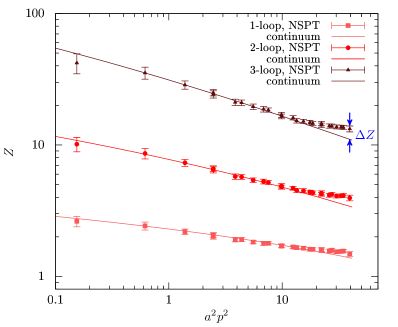
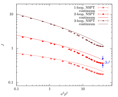
Figure 1: NSPT data for the gluon (left) and ghost (right) dressing functions for diagonal lattice momenta up to 3-loop order. Curves represent the $a\to 0$ result (see text). Arrows mark the hypercubic lattice artifacts.

To get the desired hypercubic corrections, we have to calculate the Landau-gauge gluon and ghost propagators in NSPT. Details for this can be found in [12, *DiRenzo2010cs]. Here it suffices to mention that their tensor structure (for the Wilson gauge action) is of the familiar form

$$D_{\mu\nu}^{ab}=\left(\delta_{\mu\nu}-\frac{\hat{p}_{\mu}\,\hat{p}_{\nu}}{\hat{p}^{2}}\right)\delta^{ab}\frac{Z}{\hat{p}^{2}}\qquad\text{and}\qquad G_{\mu\nu}^{ab}=\delta_{\mu\nu}\delta^{ab}\frac{J}{\hat{p}^{2}}$$ (2)

where $\hat{p}_{\mu}=\frac{2}{a}\sin(a\,p_{\mu}/2)$ denotes the eigenvalues of the free lattice Laplacian. The results are obtained in orders of $g_{0}^{2}$, because the $SU(3)$ link fields $U_{x,\mu}$ are kept as an expansion in powers of $\beta=2N_{c}/g_{0}^{2}$ which also requires algebraic operations to be performed with respect to this perturbative structure for operators $A$ and $B$:

$$U_{x,\mu}=1+\sum_{k\geq 1}\beta^{-k/2}U_{x,\mu}^{(k)}\text{,}\qquad(A+B)^{(k)}=A^{(k)}+B^{(k)}\text{,}\qquad(A\,B)^{(k)}=\sum_{j=0}^{k}A^{(k)}\,B^{(k-j)}\text{.}$$ (3)

Furthermore, the framework of NSPT relies on stochastic quantization. This is implemented by adding an artificial time $\tau$ to the gauge fields whose evolution in $\tau$ is governed by a Langevin equation, which is solved numerically. A suitable Euler scheme reads

$$U_{x,\mu}(\tau+\epsilon)=\exp\{-i\,\epsilon\,\nabla_{U_{x,\mu}}S[U]+\sqrt{\epsilon}\,\eta_{x}(\tau)\}\,U_{x,\mu}(\tau)\text{,}$$ (4)

where $\eta=\eta^{a}t^{a}$ is a random gaussian distributed $su(3)$ field ($t^{a}$ being the generators of $SU(3)$) and $S[U]$ (in our case) the Wilson plaquette action. $\nabla_{U_{x,\mu}}$ is the discretized left Lie derivative with respect to $U_{x,\mu}$. Since the Euler time step $\epsilon$ has to be finite, simulations have to be performed for several $\epsilon$ such that at the end the limit $\epsilon\rightarrow 0$ can be taken.

We choose $\epsilon=0.03$, 0.02 and 0.01 for all our simulations and collect data for $J^{(l)}$ and $Z^{(l)}$ for $l=1,\ldots,4$ loops after fixing $U_{x,\mu}$ to Landau gauge. We will focus here on diagonal lattice momenta and our lattice sizes are $8^{4}$, $16^{4}$, $24^{4}$ and $32^{4}$. Data for a $48^{4}$ lattice is in progress.

In Figure 1 we show our NSPT data for the gluon and ghost dressing functions up to 3-loop order. As we are interested in the hypercubic lattice corrections for diagonal lattice momenta we only show points for these momenta and compare it to the momentum dependence

$$J^{(i)}_{cont}(a^{2}\,p^{2})=j^{(i)}_{0}+\sum_{k=1}^{i}j^{(i)}_{k}\left(\log(a^{2}\,p^{2})\right)^{k}\text{.}$$ (5)

expected in the limit $a\to 0$ (for simplicity we write $J$ meaning both $J$ and $Z$). For the 1-loop curve we use the well-known coefficients, $j^{(1)}_{0}$ and $j^{(1)}_{1}$, from [14], while for the 2-loop and 3-loop curves we use the coefficients $j^{(i=2,3)}_{k>0}$ multiplying the divergent logarithms from 3-loop continuum perturbation theory [15], and the finite $j^{(i)}_{0}$ from our fits (see below). Within errors our values for the latter agree with those found in [12, *DiRenzo2010cs]. For a better illustration, we have marked the momentum-dependent hypercubic lattice corrections $\Delta Z$ and $\Delta J$ in Figure 1 which we aim to quantify:

$$\Delta J^{(i)}=J^{(i)}_{lat}(a^{2}p^{2},a^{4}p^{[4]},a^{6}p^{[6]},a^{8}p^{[8]})-J^{(i)}_{cont}(a^{2}\,p^{2})\text{.}$$ (6)

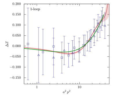
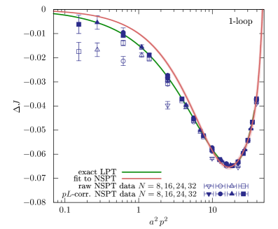
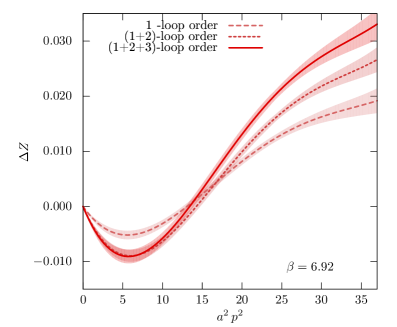
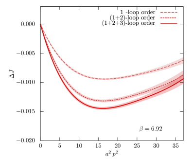
Figure 2: Hypercubic lattice artifacts at 1-loop order for the gluon (left) and ghost (right) dressing functions. $pL$-corrected (uncorrected) data is shown by full (open) symbols. Green curves are the exact 1-loop LPT results from [11]. Red bands are from a fit to the data.

Figure 3: Hypercubic lattice artifacts up to 3-loop order for the gluon (left) and ghost (right) dressing functions at $\beta=6.92$. Bands result from a fit to our NSPT data.

Removal of finite size effects

Although a first look at Figure 1 suggests we will get $\Delta Z$ and $\Delta J$ straightaway, a closer inspection of the raw data reveals we have to carefully treat finite size effects first. These are visible in particular for the ghost propagator at small momenta (see, e.g., the open symbols in Figure 3).

To treat these effects we follow a procedure proposed in [12, *DiRenzo2010cs], albeit in a slightly different manner. It starts with the observation that an observable $O$ on the lattice only depends on dimensionless quantities, namely on $ap$ (in the way as mentioned above) and on $pL$ which comes in due to the finite lattice extend $N=L/a$:

$$O(p\,a,p\,L)=O(p\,a,\infty)+\delta O(p\,a,p\,L)\text{.}$$ (7)

To get $O$ in the infinite volume limit one can either extrapolate data for several volumes or calculate and subtract $\delta O(p\,a,p\,L)$ from the data. We choose the latter, which is more robust in our case, and determine $\delta O(p\,a,p\,L)$ in the following way, similarly to [12, *DiRenzo2010cs]: We assume we can neglect the influence of additional (hypercubic) $p\,a$-corrections to $\delta O$, i.e., $\delta O(p\,a,p\,L)\approx\delta O(0,p\,L)$. This quantity then only depends on the integer tuple $k$ that defines the momentum $ap$, because $p_{\mu}\,L=\frac{2\,\pi\,k_{\mu}}{N\,a}N\,a=2\,\pi\,k_{\mu}\text{.}$ Furthermore, an observable $O(pa,\infty)$ is expected to be equal for equal physical momenta, i.e., for equal $k/N$. That is, the difference must be due to the finite-size effect and we can write:

1. $\delta O(k,N_{1})=\delta O(k,N_{2})$

2. $\delta O(k_{1},N_{1})=O(k_{1},N_{1})-\left[O(k_{2},N_{2})-\delta O(k_{2},N_{2})\right]$   if $k_{1}/N_{1}=k_{2}/N_{2}$ .

This allows us to go through our data along sequences of links (paths), each connecting two data points of either constant $k/N$ or $k$, and to get the $p\,L$-error for each path recursively. As a starting point for this recursion we choose $\delta O(k_{max},N_{max})=0$ which should be valid for large $N_{max}$.

By that procedure we can reach nearly all pairs of $(k,N)$. Most of them can be accessed by many different paths over which we average. The $pL$-error of points that are disconnected from the anchor $(k_{max},N_{max})$ is interpolated linearly between neighbouring values of $k/N$.

This method of finite-size corrections turns out to be very successful. To demonstrate that we show in Figure 3 (right) our 1-loop data for the uncorrected (open symbols) and the $pL$-corrected (full symbols) difference $\Delta J$ (Eq. (6)). There we see, finite size errors have quite an effect at low momenta and it is necessary to remove them, but after the $pL$-correction the $\Delta J$ data from different lattices falls on top of the curve one knows exactly from 1-loop LPT (from [11]).

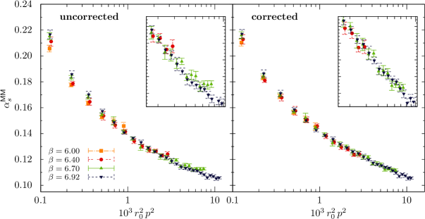
Figure 4: Coupling constant in the Minimal MOM scheme for quenched QCD in Landau gauge. Data is for a fixed physical volume (from [11]), before (left) and after (right) correcting for discretization effects.

The gluon propagator data is currently too noisy for a removal of $pL$-effects and it thus remains uncorrected in what follows. Though, within errors, points lie on the 1-loop LPT curve already.

Results

Now, that we have checked that our 1-loop NSPT results conform with the exact from LPT, we can quantify the hypercubic lattice artifacts (Eq. (6)) up to 3-loop order. To ease their later use we will provide them in a parametrization independent of the lattice coupling $\beta$. For this we fit each order separately to a polynomial of the $H(4)$ invariants:

$$\Delta J^{(i)}(p^{2},p^{[4]},p^{[6]},p^{[8]})=c_{2}\,p^{2}+c_{4}\,p^{[4]}+c_{6}\,p^{[6]}+c_{8}\,p^{[8]}\text{.}$$ (8)

The (summed-up) hypercubic lattice artifacts are then obtained for each value of $\beta$ from:

$$\Delta J(\beta,p^{2},p^{[4]},p^{[6]},p^{[8]})=\sum_{i=1}^{3}\beta^{-i}\Delta J^{(i)}(p^{2},p^{[4]},p^{[6]},p^{[8]})\text{.}$$ (9)

A comparison with the exact 1-loop LPT result from [11] shows that these fits describe the overall momentum dependence quite well, even though it cannot describe it perfectly (see Figure 3). There the fit is dominated by the many points at higher momentum while being constrained to zero at $a^{2}p^{2}=0$. So there are small deviations for small $a^{2}p^{2}$. We therefore regard this fit model not as best but as best usable to parametrize the leading hypercubic artifacts.

The final results for $\Delta Z$ and $\Delta J$ can be seen in Figure 3. There we choose $\beta\equiv 6.92$ and one sees that even for this fine lattice ($a\approx 0.026\,\text{fm}$) the 3-loop order correction still contributes rather significantly to the gluon dressing function. The ghost dressing function needs improvement to at least 2-loop order. This explains why a 1-loop correction of the data for $\alpha_{s}^{\mathsf{MM}}$ is insufficient as seen in [11]. Our new results allows us now to correct the hypercubic lattice artifacts up to 3-loop order, and, as evidenced in Figure 4, with these we are successful: The corrected $\alpha_{s}^{\mathsf{MM}}$ data (from [11]) for the different lattice spacings falls on top of each other for all momenta. Renormalization-group invariance is thus restored.

Comparison with the H(4)-Method

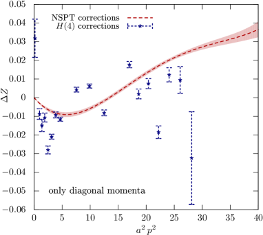
Figure 5: Hypercubic corrections for the gluon dressing function for diagonal momenta ($64^{4}$ lattice at $\beta=6.92$). Blue crosses are from the $H(4)$-method, using all available orbits (not shown). The curve is the 3-loop correction from NSPT.

It is interesting to compare our approach to the above-mentioned $H(4)$-method. With this, one tries to fit the coefficients $c_{i}$ of the hypercubic expansion of $O(ap)$, e.g., truncated at $\mathcal{O}(a^{4})$,

$$O(a\,\hat{p})=O(a^{2}\,p^{2})+c_{2}\,a^{2}\frac{p^{[4]}}{p^{2}}+c_{4}\,a^{4}\,p^{[4]}+\cdots\text{.}$$ (10)

regarding $O(a^{2}p^{2})$ as the discretization-artifacts-free operator [1, *Becirevic:1999hj, *Boucaud2003, *Soto2007]. A simultaneous fit of all the $c_{i}$’s in (10) requires many degenerate $H(4)$ orbits for nearby $a^{2}p^{2}$, that is this method works best for intermediate momenta on large lattices. For a fair comparison, we therefore choose a $64^{4}$ lattice, for which we have data for $Z$ for many different orbits. Looking again at diagonal momenta, we find the $H(4)$ correction scatter, where available, around our 3-loop NSPT correction (see Figure 5).

Conclusion

We have developed a new way to determine and remove discretization errors which are present in any lattice observable due to the hypercubic lattice symmetry. Our method is based on a perturbative calculation in the framework of NSPT, and a first application to quenched data for the Minimal MOM coupling in Landau gauge has been very successful (see Figure 4).

Our method can easily be extended, for instance, to aid calculations of renormalization constants for hadronic operators. It is planned to test this next. More details on our approach will be given in a forthcoming article.

- [1] D. Becirevic, P. Boucaud, J. Leroy, J. Micheli, O. Pene, et al., Phys.Rev. D60, 094509 (1999), arXiv:hep-ph/9903364 [hep-ph]
- [2] D. Becirevic, P. Boucaud, J. Leroy, J. Micheli, O. Pene, et al., Phys.Rev. D61, 114508 (2000), arXiv:hep-ph/9910204 [hep-ph]
- [3] P. Boucaud, F. de Soto, J. Leroy, A. Le Yaouanc, J. Micheli, et al., Phys.Lett. B575, 256 (2003), arXiv:hep-lat/0307026 [hep-lat]
- [4] F. de Soto and C. Roiesnel, JHEP 0709, 007 (2007), arXiv:0705.3523 [hep-lat]
- [5] M. Göckeler et al., Phys.Rev. D82, 114511 (2010), arXiv:1003.5756 [hep-lat]
- [6] M. Constantinou, M. Costa, M. Göckeler, R. Horsley, H. Panagopoulos, et al., Phys.Rev. D87, 096019 (2013), arXiv:1303.6776 [hep-lat]
- [7] M. Constantinou et al.(2013), arXiv:1310.6504 [hep-lat]
- [8] M. Brambilla and F. Di Renzo(2013), arXiv:1310.4981 [hep-lat]
- [9] L. von Smekal, R. Alkofer, and A. Hauck, Phys.Rev.Lett. 79, 3591 (1997), arXiv:hep-ph/9705242
- [10] L. von Smekal, K. Maltman, and A. Sternbeck, Phys.Lett. B681, 336 (2009), arXiv:0903.1696
- [11] A. Sternbeck, K. Maltman, M. Müller-Preussker, and L. von Smekal, PoS LATTICE2012, 243 (2012), arXiv:1212.2039 [hep-lat]
- [12] F. Di Renzo, E.-M. Ilgenfritz, H. Perlt, A. Schiller, and C. Torrero, Nucl.Phys. B831, 262 (2010), arXiv:0912.4152 [hep-lat]
- [13] F. Di Renzo, E.-M. Ilgenfritz, H. Perlt, A. Schiller, and C. Torrero, Nucl.Phys. B842, 122 (2011), arXiv:1008.2617 [hep-lat]
- [14] H. Kawai, R. Nakayama, and K. Seo, Nucl.Phys. B189, 40 (1981)
- [15] J. Gracey, Nucl.Phys. B662, 247 (2003), arXiv:hep-ph/0304113 [hep-ph]