Finite time interaction quench in a Luttinger model

Abstract

We analyze the dynamics of a Luttinger model following a quench in the electron-electron interaction strength, where the change in the interaction strength occurs over a finite time scale $\tau$. We study the Loschmidt echo (the overlap between the initial and final state) as a function of time, both numerically and within a perturbation scheme, treating the change in the interaction strength as a small parameter, for all $\tau$. We derive the corrections appearing in, a.) the Loschmidt echo for a finite quench duration $\tau$, b.) the scaling of the echo following a sudden ($\tau\to 0$) quench, and c.) the scaling of the echo after an adiabatic ($\tau\to\infty$) quench. We study in detail, the limiting cases of the echo in the early time and infinite time limit, and provide scaling arguments to understand these in a general context. We also show that our perturbative results are in good agreement with the exact numerical ones.

I Introduction

There is a recent upsurge in the studies of non-equilibrium dynamics of quantum many body systems polkovnikov11 ; dutta10 ; dziarmaga10 driven across a quantum critical point (QCP) or gapless critical regions sachdev99 . Possibility of experimental realization in cold atomic systems coldatom_1 ; polkovnikov11 has paved the way for a plethora of theoretical works to investigate the time dependent evolution and detection of quantum many body systems. In particular, quenching of interactions by means of Feshbach resonances or changing the lattice parameters as a function of time has motivated numerous theoretical polkovnikov11 and experimental works coldatom_3 .

In this article, we explore the behaviour of the Loschmidt echo (LE), which is defined as the overlap of wave functions, $|\Psi_{0}(t)\rangle$ and $|\Psi(t)\rangle$, evolving from the same initial state, but with different Hamiltonians $H_{0}$ and $H$, respectively. It is given by

$$\mathcal{L}(t)=\left|\langle\Psi_{0}|e^{iH_{0}t}e^{-iHt}|\Psi(t)\rangle\right|^{2},$$ (1)

and is usually interpreted as a measure of the hyper-sensitivity of the time evolution of the system to the perturbations experienced due to the surrounding environment peres ; scholar . It is also interpreted as the time evolved fidelity following a quantum quench pollmann10 ; heyl13 in the sense that $\mathcal{L}(t)$ measures the overlap between the initial ground state $|\Psi_{0}\rangle$ (of $H_{0}$) and the corresponding time evolved state $|\Psi(t)\rangle=e^{-iHt}|\Psi_{0}\rangle$, when $H_{0}$ is changed to $H$ . In the context of a quantum phase transition, the LE has been found useful in detecting a QCP showing a sharp dip in its vicinity quan06 ; sharma12 ; it also shows an early time decay with the decay constant characterized by the critical exponents of the associated quantum phase transition fazio_pra . In recent years the LE, which is also related to the orthogonality catastrophe, has been probed experimentally Knapp_PRX . Although the temporal evolution of the echo following a quantum quench across a QCP has been studied in several works silva08 ; pollmann10 ; damski11 ; Venuti ; damski11_2 ; nag12 ; heyl13 , the same when the quantum system is quenched within a gapless critical phase has gained more prominence in recent times cazalila_prl06 ; Perfetto_epl ; Dora_prl_2011 ; Dora_prl13 ; Dora3 ; Meden2 ; meden_prl12 .

In this work, we focus on a paradigmatic one dimensional interacting system with a gapless phase, namely the Luttinger model LL_ref (LM) which is characterized by bosonic collective modes as elementary excitations. LM can be seen as a fixed point, in the renormalization group sense, for a large class of gapless quantum many-body systems in one dimension, i.e., the equilibrium, low energy properties of many one-dimensional systems are universally described by the LM. Interacting cold atoms in a one dimensional trap mimics such LMs coldatom_4 , as confirmed by existing experiments finitequench_1 . Other systems where LM is relevant are various spin models or interacting fermion systems fazio_pra ; dora_prb12 ; DzairmagaPRB2011 .

The LM has recently been studied from the view point of quantum quenches and thermalization cazalila_prl06 ; LL_quench2 ; aditi_prl11 ; aditi_prl12 . Here, we study the non-equilibrium properties of a LM, due to a change in the interaction parameter achieved over finite span of time given by $\tau$, investigating the behaviour of the LE. In particular we will focus on an interaction quench in a LM using a linear protocol from an initial state to a final state.

The paper is organized in the following manner. In Sec II, we introduce the model Hamiltonian, i.e. LM, with an interaction quench, and calculate the Loschmidt echo; within the central spin model, where a qubit is coupled to a quantum many body system, the LE measures the decoherence of the qubit quan06 . In Section III, we reproduce the limiting behaviour of the LE for sudden ($\tau\to 0$) and adiabatic quench ($\tau\to\infty$), where we also argue that the result in the adiabatic case can also be interpreted by visualizing an adiabatic quench as a process that leads to the formation of an interacting Luttinger liquid from a non interacting 1D system. In section IV, we study the LE for a finite time linear interaction quench a.) within a perturbation scheme with quench amplitude (or the change in the interaction strength) as the small parameter and b.) numerically. In Section V, we analyze the LE in various limits, particularly focussing on the early time (immediately after quench) and asymptotic ($t\to\infty$) behaviour both for small and large $\tau$ and discuss alternate scaling arguments in a more general context. The summary and discussion of our results is presented in section VI. We note at the outset that we shall denote the LE for fast quench (small $\tau$) and slow quench (large $\tau$ limit) using the notations $\mathcal{L}_{SQ^{+}}$ and $\mathcal{L}_{AQ^{-}}$, respectively.

II Luttinger model and the Loschmidt Echo

The low energy properties of interacting 1D bosons or that of spin chains can be described in terms of bosonic sound like excitations, in the LM. The initial LM Hamiltonian, we consider is given by LL_ref

$$H_{i}=\sum_{q\neq 0}\left(v_{0}|q|b_{q}^{\dagger}b_{q}+\frac{g_{i}|q|}{2}\left[b_{q}b_{-q}+b_{q}^{\dagger}b_{-q}^{\dagger}\right]\right)~{}.$$ (2)

Here, $v_{0}|q|$ is the ‘linearized’ excitation spectrum of the non-interacting bosons, $g_{i}$ is the initial interaction strength, and $b_{q}^{\dagger}~{}(b_{q})$ is the creation (annihilation) operator describing the bosonic density excitations. The Hamiltonian in Eq.(2) being quadratic in bosonic operators can be easily diagonalized in terms of new bosonic quasiparticle operators ($\beta_{q},~{}\beta_{q}^{\dagger}$), using the standard time-independent Bogoliubov transformation $b_{q}=u_{q}~{}\beta_{q}-v_{q}~{}\beta_{-q}^{\dagger}$. The commutation relations for the bosonic operators enforce the condition, $|u_{q}|^{2}-|v_{q}|^{2}=1$, which enable us to use the parameterization, $u_{q}\equiv\cosh(\phi_{q})$, and $v_{q}\equiv\sinh(\phi_{q})$. One can easily arrive at the condition that diagonalizes Hamiltonian (2), given by,

$$\tanh(2\phi_{q})=\frac{g_{i}}{v_{0}}~{}~{}~{}{\rm or}~{}~{}~{}e^{-2\phi_{q}}=\left(\frac{v_{0}-g_{i}}{v_{0}+g_{i}}\right)^{1/2}\equiv K_{i}~{}.$$ (3)

Here $K_{i}$ is the dimensionless LM interaction parameter which characterises the initial strength of interaction. Note that $K_{i}=1$ for a non interacting system, $K_{i}<1$ for repulsive ($g_{i}>0$) electron electron interactions and $K_{i}>1$ for attractive ($g_{i}<0$) electron electron interactions. The Bogoliubov coefficients can be expressed as

$$u_{q} = \frac{\sqrt{v_{0}+g_{i}}+\sqrt{v_{0}-g_{i}}}{2(v_{0}^{2}-g_{i}^{2})^{1/4}}=\frac{K_{i}+1}{2\sqrt{K_{i}}}~{},~{}~{}~{}{\rm and}$$ (4)

$$v_{q} = \frac{\sqrt{v_{0}+g_{i}}-\sqrt{v_{0}-g_{i}}}{2(v_{0}^{2}-g_{i}^{2})^{1/4}}=\frac{K_{i}-1}{2\sqrt{K_{i}}}~{}.$$ (5)

The diagonalised Hamiltonian in terms of new bosonic operators is given by

$$H_{i}=\varepsilon_{i}+\sum_{q\neq 0}v_{i}|q|~{}\beta_{q}^{\dagger}\beta_{q},$$ (6)

where $v_{i}=\sqrt{v_{0}^{2}-g_{i}^{2}}$, is the renormalized velocity and $\varepsilon_{i}$ is the ground state energy of $H_{i}$ with respect to the non-interacting ground state. The initial quasiparticle dispersion spectra is given by $\omega_{i}(q)=v_{i}|q|$; clearly, the ground state of $H_{i}$ is the vacuum of the $\beta$ bosons.

To study the dynamics of the LM, we quench the interaction strength from an initial value $g_{i}$ to a final value $g_{f}$ within a quench time $\tau$. The quench in the interaction parameter is described by incorporating an additional time dependent term in the Hamiltonian [Eq.(2)]

$$H^{\prime}=\sum_{q\neq 0}\frac{\delta_{g}|q|Q(t)}{2}[b_{q}b_{-q}+b_{q}^{\dagger}b_{-q}^{\dagger}],$$ (7)

where $\delta_{g}=g_{f}-g_{i}$, and $Q(t)$ is the quench protocol satisfying $Q(t<0)=0$ and $Q(t>\tau)=1$; the cases $\tau=0$ and $\tau\to\infty$ refer to the sudden and adiabatic quenching schemes, respectively. The time dependent Hamiltonian ($H=H_{i}+H^{\prime}$), can now be recast in terms of the $\beta$ bosons using the standard Bogoliubov transformation ($b_{q}=u_{q}\beta_{q}-v_{q}\beta_{-q}^{{\dagger}}$) to the form:

$$H(t)=\varepsilon_{i}+\sum_{q\neq 0}\left\{\left(v_{i}-\frac{g_{i}\delta_{g}Q(t)}{v_{i}}\right)|q|\beta_{q}^{\dagger}\beta_{q}+\right.$$

$$\left.+\frac{\delta_{g}Q(t)v_{0}}{2v_{i}}|q|[\beta_{q}\beta_{-q}+\beta_{q}^{\dagger}\beta_{-q}^{\dagger}]-\frac{\delta_{g}Q(t)g_{i}}{v_{i}}|q|\right\}~{}.$$ (8)

Redefining the time-dependent parameters as $v(t)=(v_{i}-\delta_{g}Q(t)g_{i}/v_{i})$, and $g(t)=(\delta_{g}Q(t)v_{0}/v_{i})$, and ignoring unimportant constants, one finds

$$H(t)=\sum_{q\neq 0}\left(v(t)|q|~{}\beta_{q}^{\dagger}\beta_{q}+\frac{g(t)|q|}{2}\left[\beta_{q}\beta_{-q}+\beta_{q}^{\dagger}\beta_{-q}^{\dagger}\right]\right)\;.$$ (9)

The time evolution for the quadratic Eq.(9) is obtained by the Heisenberg equation of motion, leading to

$$i\partial_{t}\beta_{q} = v(t)|q|~{}\beta_{q}(t)+g(t)|q|~{}\beta_{-q}^{\dagger}(t)~{},$$

$$i\partial_{t}\beta_{-q}^{\dagger}(t) = -v(t)|q|~{}\beta_{-q}^{\dagger}(t)-g(t)|q|~{}\beta_{q}(t)~{}.$$ (10)

The coupled linear Eq.(10) have solutions of the following form

$$\beta_{q}(t)=f(q,t)~{}\beta_{q}(0)+h^{*}(q,t)~{}\beta^{\dagger}_{-q}(0)~{},$$ (11)

where the time-dependence has been completely shifted to the pre-factors $f(q,t)$ and $h(q,t)$ which satisfy the condition $|f(q,t)|^{2}-|h(q,t)|^{2}=1$ for all times. Also, the operators $\beta_{q}(0)$ and $\beta_{q}^{\dagger}(0)$, appearing on the right hand side of Eq.(11) defined, at time $t=0$, refer to non-interacting Bogoliubov bosons describing the initial Hamiltonian in Eq.(6). Using Eqs.(10)-(11), we obtain coupled differential equations for the coefficients $f(q,t)$ and $h(q,t)$, satisfying

$$i\partial_{t}\left[\begin{array}[]{c}f(q,t)\\ h(q,t)\end{array}\right]=|q|\times\left[\begin{array}[]{cc}v(t)&g(t)\\ -g(t)&-v(t)\end{array}\right]\left[\begin{array}[]{c}f(q,t)\\ h(q,t)\end{array}\right]~{}.$$ (12)

with the initial condition $[f(q,0),~{}h(q,0)]=[1,~{}0]$.

Using the generic definition given in Eq.(1), one can find the LE or the overlap of wave functions time evolved from the initial ground state with the Hamiltonian $H_{i}$ and the time dependent Hamiltonian $H(t)$ [Eq. (9)], respectively. This has been calculated for a spin-less Luttinger model in Ref. [Dora_prl13, ], and is expressed in terms of the time dependent coefficients $[f(q,t),h(q,t)]$ as,

$$\mathcal{L}(t)=\exp{\left[-\sum\limits_{q>0}~{}\ln\left(|f(q,t)|^{2}\right)\right]}~{}.$$ (13)

In subsequent sections, we solve Eq.(12) to obtain $[f(q,t),h(q,t)]$ and hence the LE in different situations.

III Loschmidt echo in the adiabatic and the sudden quench limit

Before discussing the LE for a finite time quench, let us briefly reproduce the behaviour of the LE for the limiting cases of adiabatic and sudden quench reported in Ref.[Dora_prl13, ]. We reiterate that we are varying the interaction strength from $g_{i}$ to $g_{f}$ in a finite interval of time $\tau$; $\tau\to\infty$ ($\tau=0$) limit correspond to the adiabatic (sudden) case. For convenience, let us also define the final renormalized velocity, $v_{f}=(v_{0}^{2}-g_{f}^{2})^{1/2}$, and the final dispersion relation, $\omega_{f}(q)=v_{f}|q|$.

III.1 Adiabatic quench

In the adiabatic limit, after the quench ($t>\tau\to\infty$, i.e., $Q(t)=1$), Eq.(12) has stationary solutions of the form $[f(q,t),h(q,t)]=[f_{q},h_{q}]e^{-i\omega_{f}(q)t}$. These solutions in Eq.(12) together with the final expression for the velocity and interaction strength, $v(t>\tau)=(v_{0}^{2}-g_{f}g_{i})/v_{i}$ and $g(t>\tau)=(g_{f}-g_{i})v_{0}/v_{i}$, leads to

$$|f(q,t>\tau)|^{2}=\frac{1}{2}+\frac{1}{4}\left(\frac{K_{f}}{K_{i}}+\frac{K_{i}}{K_{f}}\right)~{}.$$ (14)

Here we have used the constraint $|f_{q}|^{2}-|h_{q}|^{2}=1$ and the parameter $K_{f}=\sqrt{[v_{0}-g_{f}]/[v_{0}+g_{f}]}$ characterizes the strength of interaction in final state. The LE can now be obtained by substituting Eq.(14) in Eq.(13), and is given by

$$\mathcal{L}_{AQ}=\left(\frac{1}{2}+\frac{1}{4}\left(\frac{K_{f}}{K_{i}}+\frac{K_{i}}{K_{f}}\right)\right)^{-L/2\pi\alpha}~{},$$ (15)

where $L$ is the system size and the momentum sum in the exponential has been regularized using the ultraviolet cut-off $1/\alpha$. Here $\alpha$ is a non-universal and model-dependent short distance cutoff (inverse of the ultraviolet cutoff) which is used for the regularization of divergences in the Luttinger model. Since $1/\alpha$ is a measure of the maximum wave vector included in the sum of Eq.(13), and the separation between any two wave vectors is $2\pi/L$, the exponent $L/(2\pi\alpha)$, appearing in the Loschmidt Echo, just represents the number of wave vectors appearing in the sum of Eq.(13). The soft cutoff $\alpha$ arises, naturally when any finite size physical system is mapped to the Luttinger model. For example in the $XXZ$ model, $L/(2\pi\alpha)=\pi^{2}N\chi_{f}$, where $N$ is the number of lattice sites, and, $\chi_{f}$ is the knownsirker_prl10 , fidelity susceptibility around the non-interacting $XX$ point of the $XXZ$ model Dora_prl13 . In the present study, the cut-off renormalizes the length of $L$ of the system and the scaling relations derived here depend on the rescaled length $L/\alpha$.

Clearly the adiabatic LE simply measures the overlap of the ground state of initial and final Hamiltonians implying that in the adiabatic limit the system is always in its instantaneous ground state which can be viewed as the ground state of an instantaneous LM with a time dependent effective interaction parameter

$$K(t)=\sqrt{\frac{v(t)-g(t)}{v(t)+g(t)}}~{}.$$ (16)

One can also use this argument to arrive at the result given in Eq. 15. Using Eq.(16) in Eq.(4), for $t>\tau$, i.e., when $v(t)=(v_{0}^{2}-g_{f}g_{i})/v_{i}$ and $g(t)=(g_{f}-g_{i})v_{0}/v_{i}$, one can find out the time independent Bogoliubov coefficient,

$$|u_{q}|^{2}=\frac{1}{2}+\frac{1}{4}\left(\frac{K_{f}}{K_{i}}+\frac{K_{i}}{K_{f}}\right)~{}.$$ (17)

After the quench, $|u_{q}|^{2}=|f(q,t>\tau)|^{2}$ as the interaction parameter is no longer changing and there is no mixing of the $\pm q$ modes [see Eq.(11)], and this leads to Eq.(15).

We note in passing that the argument presented above is also consistent with the idea behind the ‘formation’ of an interacting Luttinger liquid state starting from an initial non-interacting state, $K_{i}=1$, by adiabatically switching on the interactions. Technically this is evident by substituting $K_{i}\to 1$ and $K_{f}\to K_{i}$ in Eq.(17) which immediately leads to Eq.(4). We note that the adiabatic LE turns out to be the modulus squared of the ground state fidelity, and Eq.(15) is consistent with the ground state fidelity calculated earlier fidelity_yang .

III.2 Sudden quench

In the sudden quench limit ($\tau\to 0$), for $t>0$, the velocity and the interaction strength assume their time independent final value, and Eq.(12) can be decoupled to obtain $\partial_{t}^{2}f(q,t)+v_{f}^{2}|q|^{2}f(q,t)=0$. Solving this with the initial condition, $f(q,0)=1$, we get

$$f(q,t)=\cos(v_{f}|q|t)-\frac{i}{2}\left(\frac{K_{f}}{K_{i}}+\frac{K_{i}}{K_{f}}\right)\sin(v_{f}|q|t)~{}.$$ (18)

(An identical result has also been derived in Ref.[cazalila_prl06, ] using forward Bogoliubov transformation which is followed by the backward one). Using Eq.(18), we find the decay in the LE in the very short time limit ($t\ll\alpha/v_{f}$)) given by

$$\mathcal{L}_{SQ}(t)\approx\exp\left[-\frac{L}{2\pi\alpha}\left(\frac{K_{f}}{K_{i}}-\frac{K_{i}}{K_{f}}\right)^{2}\frac{v_{f}^{2}t^{2}}{12\alpha^{2}}\right]~{}.$$ (19)

We note that this is the usual gaussian decay of a LE expected (from a perturbation theory point of view) for a sudden quench peres ; fazio_pra .

In the large time limit ($t\gg\alpha/v_{f}$), on the other hand, one can neglect a small oscillating term with decaying amplitude (as $t$ increases), to obtain a simplified time independent form of the echo,

$$\mathcal{L}_{SQ}(t\gg\alpha/v_{f})=\left(\frac{1}{2}+\frac{1}{4}\left(\frac{K_{f}}{K_{i}}+\frac{K_{i}}{K_{f}}\right)\right)^{-L/\pi\alpha}~{}.$$ (20)

We emphasize that in the long time $t\rightarrow\infty$ limit, $\mathcal{L}_{SQ}=\mathcal{L}_{AQ}^{2}$; this correspondence has been reported in the Ref. [Dora_prl13, ] (also see Ref. [Heyl13, ]). In the adiabatic limit, $\mathcal{L}_{AQ}=|\langle G_{f}|G_{0}\rangle|^{2}$ where $G_{0}$ and $G_{f}$ are the ground states of the initial and final Hamiltonian, respectively. On the other hand, in the sudden limit, the LE takes the form $\mathcal{L}=|\langle\Phi(t)|\Phi_{0}(t)\rangle|^{2}=|\langle G_{0}|e^{iHt}e^{-iH_{0}t}|G_{0}\rangle|^{2}$. When expanded in eigenstates of final Hamiltonian, only the ground state contributes to LE in the asymptotic limit, while the oscillating terms due to the excited states interfere destructively and vanish as $t\rightarrow\infty$; one therefore finds $\mathcal{L}_{SQ}|_{t\to\infty}=|\langle G_{f}|G_{0}\rangle|^{4}$, thereby yielding the correspondence $\mathcal{L}_{SQ}=\mathcal{L}_{AQ}^{2}$.

IV Loschmidt Echo for the finite time linear quench

In this section we focus on the interaction quench in a LM from an initial value $g_{i}$ to a final value $g_{f}$ introduced over a finite interval time $\tau$ using the quenching protocol,

$$Q(t\leq 0)=0,~{}~{}~{}Q(0<t<\tau)=t/\tau~{}~{}{\rm and}~{}~{}Q(t\geq\tau)=1.$$

We use Eq.(12) which can be decoupled in different regimes. For all quenching schemes, we get

$$\ddot{f}+v_{i}^{2}q^{2}f=0~{}~{}~{}{\rm and}~{}~{}~{}\ddot{h}+v_{i}^{2}q^{2}h=0~{},$$ (21)

for $t<0$ while for $t\geq\tau$

$$\ddot{f}+v_{f}^{2}q^{2}f=0~{}~{}~{}{\rm and}~{}~{}~{}\ddot{h}+v_{f}^{2}q^{2}h=0~{}.$$ (22)

where we have dropped the arguments $q,t$ for $f(q,t)$ and $h(q,t)$. However for the quenching scheme we are interested in, we have the following set of coupled equations during the interval $0<t<\tau$  i.e., when the interaction is being quenched

$$\ddot{f}-\frac{\dot{f}}{t}+\left[v_{0}^{2}q^{2}-\left(g_{i}+\delta_{g}t/\tau\right)^{2}q^{2}-i\frac{v_{i}|q|}{t}\right]f = 0~{},$$

$$\ddot{h}-\frac{\dot{h}}{t}+\left[v_{0}^{2}q^{2}-\left(g_{i}+\delta_{g}t/\tau\right)^{2}q^{2}+i\frac{v_{i}|q|}{t}\right]h = 0~{}.$$

We solve these linear second order inhomogeneous equation using numerical techniques. However, we also consider the case when the change in the interaction parameter $\delta_{g}$ is small and employ a perturbative expansion in $\delta_{g}\to 0$, to gain insight of the time-evolution of the LE following a linear quench. We emphasize that the $\delta_{g}\to 0$ limit happens to be analogous to the adiabatic quench regime of $\tau\to\infty$, as only the combination of $\delta_{g}/\tau$ appears in Eq.(IV).

We now find the perturbative solutions of Eq.(12) [or equivalently Eq.(IV)], with the boundary conditions $[f(q,t=0),h(q,t=0)]=[1,0]$, in terms of the small interaction parameter, i.e., $\delta_{g}<<v_{i}$. The solutions of Eq.(22) are just harmonically varying functions of constant frequency ($\omega_{f}$), whose constant coefficients need to be determined through boundary condition at $t=\tau$; this necessitates solving Eq.(IV) to obtain the value of the functions $[f(q,\tau),h(q,\tau)]$.

Solution for $t<\tau$ (i.e., within the interval during which the interaction term is being changed): using Eq.(12), we get Dora_prl_2011 to lowest order in $\delta_{g}$, i.e., ${\cal O}(\delta_{g})$,

$$f(q,0<t<\tau) \approx \text{exp}(-iv_{i}|q|t)$$

$$h(q,0<t<\tau) \approx \frac{i\delta_{g}v_{0}|q|}{v_{i}\tau}~{}e^{i[v_{i}t-\frac{\delta_{g}g_{i}}{2v_{i}\tau}t^{2}]|q|}$$ (24)

$$\times \int_{0}^{t}t^{\prime}e^{-2iv_{i}|q|t^{\prime}}e^{i\frac{\delta_{g}g_{i}|q|}{2v_{i}\tau}t^{\prime 2}}dt^{\prime}~{}.$$

The integral on the RHS of above equation can be evaluated exactly to obtain,

$$h(q,t) = \frac{v_{0}}{g_{i}}~{}e^{-i\left(2v_{i}^{2}t+\frac{g_{i}\delta_{g}t^{2}}{\tau}+\frac{4v_{i}^{4}\tau}{g_{i}\delta_{g}}\right)\frac{|q|}{2v_{i}}}\Bigg{[}e^{\frac{2iv_{i}^{3}\tau|q|}{g_{i}\delta_{g}}}\left(-e^{2iv_{i}|q|t}+e^{\frac{ig_{i}\delta_{g}|q|t^{2}}{2v_{i}\tau}}\right)+(1+i)~{}e^{2iv_{i}|q|t}$$ (25)

$$\times v_{i}\sqrt{\frac{\pi\tau v_{i}|q|}{g_{i}\delta_{g}}}\Bigg{\{}\mathbf{Erfi}\left(\frac{(1+i)v_{i}\sqrt{v_{i}|q|\tau}}{\sqrt{g_{i}\delta_{g}}}\right)+\mathbf{Erfi}\left(\frac{(1+i)(g_{i}\delta_{g}t-2v_{i}^{2}\tau)\sqrt{|q|}}{2\sqrt{g_{i}\delta_{g}v_{i}\tau}}\right)\Bigg{\}}\Bigg{]},~{}$$

where $\mathbf{Erfi}(z)=-i~{}\mathbf{Erf}(iz)$, is the imaginary error function. We expand the expression in Eq.(25) in powers of $\delta_{g}$, retaining only the lowest order term. This simplifies Eq.(25) upto ${\cal O}(\delta_{g})$ to the form,

$$h(q,t\leq\tau)\approx\frac{\delta_{g}v_{0}}{2v_{i}^{2}}\left(\frac{\sin(v_{i}|q|t)}{v_{i}|q|\tau}-\frac{t}{\tau}e^{-iv_{i}|q|t}\right)~{}.$$ (26)

Solution for $t\geq\tau$ : In order to calculate the coefficients in $t\geq\tau$ regime, i.e., after the interaction reaches its final value, we use Eq. (26) at $t=\tau$ as the boundary condition for Eq. (22) and obtain the time evolution of $h(q,t\geq\tau)$ to be

$$h(q,t\geq\tau)\approx\frac{\delta_{g}v_{0}}{2v_{i}^{2}}\left[\frac{\sin(v_{i}|q|\tau)}{v_{i}|q|\tau}e^{iv_{i}|q|(t-\tau)}-e^{-iv_{i}|q|t}\right]~{}.$$ (27)

The first term in the square brackets dominates the time evolution for small $\tau$ (i.e., $\tau<<1/\omega_{i}$), and the second term yields the time evolution for large $\tau$ (i.e., $\tau>>1/\omega_{i}$). One can readily obtain the exact results for the sudden ($\tau=0$) as well as adiabatic ($\tau=\infty$) quench limits

$$h_{SQ}(q,t\geq\tau) \approx \frac{i\delta_{g}v_{0}}{v_{i}^{2}}\sin(v_{i}|q|t)~{},~{}~{}~{}{\rm and}$$

$$h_{AQ}(q,t\geq\tau) \approx -\frac{\delta_{g}v_{0}}{2v_{i}^{2}}e^{-iv_{i}|q|t}~{},$$ (28)

to lowest order in $\delta_{g}$. Eq.(27) provides the perturbative solution of $h(q,t)$ (which in fact yields the number of excited states with respect to the vacuum of the $\beta_{q}$ bosons generated during the quenching process) in powers of $\delta_{g}$, for finite $\tau$ at all times and appropriately reduces to the sudden and adiabatic quench limits.

We now proceed to study the LE by means of the perturbative solution in powers of small parameter $\delta_{g}$. Using Eq.(27), and the constraint $|f(q,t)|^{2}-|h(q,t)|^{2}=1$, we find $|f(q,t)|^{2}$, which is then substituted in Eq.(13) to obtain the finite $\tau$ behaviour of LE for a finite time, i.e., $t\geq\tau$ in the perturbative limit:

$$\mathcal{L}(t) = \text{exp}\left[-\frac{L}{2\pi}\int_{0}^{1/\alpha}\text{ln}\left(1+\frac{\delta_{g}^{2}v_{0}^{2}}{8v_{i}^{4}}\left[\frac{1}{v_{i}^{2}q^{2}\tau^{2}}+2-\frac{\cos(2v_{i}|q|\tau)}{v_{i}^{2}q^{2}\tau^{2}}+\frac{2}{v_{i}|q|\tau}\{\sin(2v_{i}|q|(t-\tau))-\sin(2v_{i}|q|t)\}\right]\right)dq\right]~{},$$

$$\approx \text{exp}\left[-\frac{L}{2\pi\alpha}\frac{\delta_{g}^{2}v_{0}^{2}}{4v_{i}^{4}}\left(1-\frac{\alpha^{2}}{v_{i}^{2}\tau^{2}}\sin^{2}\left(\frac{v_{i}\tau}{\alpha}\right)+\frac{\alpha}{v_{i}\tau}\left\{-\text{Si}\left(\frac{2v_{i}t}{\alpha}\right)+\text{Si}\left(\frac{2v_{i}(t-\tau)}{\alpha}\right)+\text{Si}\left(\frac{2v_{i}\tau}{\alpha}\right)\right\}\right)\right]~{}.$$

In the above equation, the function $\text{Si}(x)$ is the SinIntegral of $x$ defined as $\text{Si}(x)=\int_{0}^{x}(\sin{t}/t)dt$, with $1/\alpha$ as the upper momentum (ultra-violet) cut-off. The above expression provides a generic form of the LE as a function of $\tau$ and $t$ which will be used extensively in the subsequent calculations. In the adiabatic quench case ($\tau\to\infty$), only the first term in the exponential of Eq.(LABEL:LEexp1) contributes, while in the sudden quench limit ($\tau\to 0$), the first and the second terms in the exponential of Eq.(LABEL:LEexp1) contribute, resulting in the following expressions,

$$\mathcal{L}_{AQ}(t\geq\tau) = \text{exp}\left[-\frac{L}{2\pi\alpha}\frac{\delta_{g}^{2}v_{0}^{2}}{4v_{i}^{4}}\right]~{},~{}~{}~{}{\rm and}$$ (30)

$$\mathcal{L}_{SQ}(t\geq\tau) = \text{exp}\left[-\frac{L}{2\pi\alpha}\frac{\delta_{g}^{2}v_{0}^{2}}{2v_{i}^{4}}\right]~{}.$$ (31)

which satisfy the correspondence $\mathcal{L}_{SQ}=\mathcal{L}_{AQ}^{2}$ established for an arbitrary value of $\delta_{g}$ Dora_prl13 .

In Fig.1, we plot the temporal evolution of the LE for a fast quench, with $\tau=0.2$, obtained both numerically and analytically for small $\delta_{g}$ . As anticipated earlier, we find very good agreement between the perturbative and the exact results.

The case of a slow quench, for $\tau=5$, is shown in Fig.2. Although, the quantitative agreement between the perturbative and the exact solutions is not as perfect as the small $\tau$ case, the perturbative solutions still capture all the qualitative features. However, it is worth noting that for both fast and slow quenches, the LE shows a damped oscillatory behaviour which saturates to some finite value in the infinite time limit. The dimensionless time period of these oscillations can be estimated using Eq.(LABEL:LEexp1) and is given by $T=\pi\alpha/(v_{i}\tau)$, which corresponds to a value of $5$ and $0.2$ for Fig.1 and Fig.2 respectively. The damped oscillatory nature of the LE, and its saturation to an asymptotic constant value with time, are characteristics of the LE that has also been observed following a linear quench across the QCP of a transverse Ising chain pollmann10 .

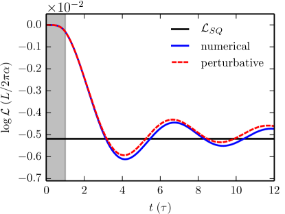
Figure 1: (Color online) Plot for $\log\mathcal{L}(t)$, in units of $L/(2\pi\alpha)$, as a function of time for $v_{i}\tau/\alpha=0.2\pi$ and $\delta_{g}/v_{i}=0.1$ for an initial choice of $g_{i}/v_{i}=0.1$ (i.e., $K_{i}=0.91$). The solid (blue) line denotes the exact numerical result [based on Eq.(12)] and the dotted(red) line shows the perturbative solution [based on Eq.(LABEL:LEexp1)]. The solid horizontal line is the analytical expression for the LE in the sudden quench limit (for $\tau\to 0$ and $t\to\infty$). The shaded region marks the ‘quench’ interval during which the interaction parameter is changed.

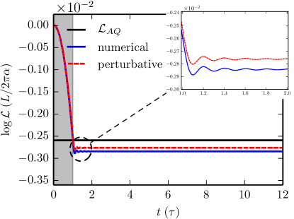
Figure 2: (Color online) Plot for $\log\mathcal{L}(t)$, in units of $L/(2\pi\alpha)$, as a function of time for $v_{i}\tau/\alpha=5\pi$ and $\delta_{g}/v_{i}=0.1$ for an initial choice of $g_{i}/v_{i}=0.1$ (i.e., $K_{i}=0.91$). The solid (blue) line denotes the exact numerical result [based on Eq.(12)] and the dotted(red) lines shows the perturbative solution [based on Eq.(LABEL:LEexp1)]. The solid horizontal line is the analytical expression for the LE in the adiabatic quench limit (for $t\to\infty$). The shaded region marks the ‘quench’ interval during which the interaction parameter is changed.

V Loschmidt Echo in different limits

In this section we focus our efforts on studying the behaviour of the LE in the early time limit immediately after the quench [$(t/\tau-1)\to 0$] and also the asymptotic large time limit [$t/\tau\to\infty$]. In particular, we will be interested in the corrections to the LE in the sudden and the adiabatic limits.

V.1 Loschmidt Echo in the early time limit

To find the early time limit after the quench, i.e., when $0<t-\tau<\alpha/v_{i}$, Eq.(LABEL:LEexp1) can be expanded in powers of $t-\tau$ (see Fig. 3). For the case of $t=\tau$, the last term in Eq.(LABEL:LEexp1) vanishes and LE simplifies to the form

$$\mathcal{L}(\tau)=\exp\left[-\frac{L}{2\pi\alpha}\frac{\delta_{g}^{2}v_{0}^{2}}{4v_{i}^{4}}\left(1-\frac{\text{sin}^{2}\left(v_{i}\tau/\alpha\right)}{v_{i}^{2}\tau^{2}/\alpha^{2}}\right)\right].~{}$$ (32)

The behaviour of the early time LE for a fast quench, i.e., in the small $\tau$ limit, can be investigated by taking the limit $\tau\to 0$ in Eq. (LABEL:LEexp1), and to the lowest order in $\tau$ for $0<t-\tau<\alpha/v_{i}$, it is given by

$$\mathcal{L}_{SQ^{+}}({t})\approx\text{exp}\left[-\frac{L}{2\pi\alpha}\frac{\delta_{g}^{2}v_{0}^{2}}{3\alpha^{2}v_{i}^{2}}\left\{t^{2}-\tau(t-\tau/4)\right\}\right].$$ (33)

Here the first term corresponds to the expected gaussian decay of the LE, with a decay constant independent of $\tau$, which is a generic feature of the LE following a quench peres ; fazio_pra . On the other hand, the second term depends on $\tau$, and indicates a correction to the proper Gaussian decay; thereby it carries a signature of the fact that the interaction has been quenched over a finite interval of time. As expected, this correction term vanishes when $\tau=0$.

For a slow quench, i.e., large $\tau$, to lowest order in $\tau$ we find the following form for the LE for all times,

$$\mathcal{L}_{AQ^{-}}(t) = \text{exp}\Bigg{[}-\frac{L}{2\pi\alpha}\frac{\delta_{g}^{2}v_{0}^{2}}{4v_{i}^{4}}\Bigg{\{}1-\frac{\text{sin}^{2}(v_{i}\tau/\alpha)}{v_{i}^{2}\tau^{2}/\alpha^{2}}$$

$$+ \frac{2(t-\tau)}{\tau}-\frac{2v_{i}^{2}}{\alpha^{2}}\frac{(t-\tau)^{2}}{\tau}\frac{\text{cos}(2v_{i}\tau/\alpha)}{2v_{i}\tau/\alpha}\Bigg{\}}\Bigg{]}~{}.$$

Here the first term in the exponential, is the echo for the adiabatic case and as expected it is independent of time and the quench rate. The expression in Eq.(LABEL:eq:slow1), can be simplified to obtain the early time behaviour for a slow quench. Retaining the most dominant correction term in $\tau$ for $0<t-\tau<\alpha/v_{i}$, we obtain:

$$\mathcal{L}_{AQ^{-}}({t})\approx\text{exp}\left[-\frac{L}{2\pi\alpha}\frac{\delta_{g}^{2}v_{0}^{2}}{v_{i}^{4}}\left\{1+2\frac{(t-\tau)}{\tau}\right\}\right]~{}.$$ (35)

We emphasise that, for a finite quench rate, we find that the correction to the early time behaviour of the LE, after a slow quench, shows a linear exponential decay in time.

The corrections to the early time behaviour of the LE due to a finite quench rate, primarily arise due to the fact that the state from which the early time behaviour is observed, i.e. $\psi(t=\tau)$, is neither a ground state of the initial Hamiltonian, nor of the final Hamiltonian. In general $\psi(t=\tau)$ incorporates ‘defects’ (excited states contributions) for a finite quench rate ($\tau$), over the initial ground state at $t=0$. This actually leads to the difference in the early time behaviour both in the large $\tau$ and small $\tau$ limits, manifested in Eqs. (37) -(39).

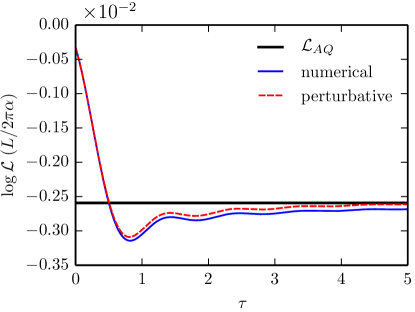
Figure 3: (Color online) Plot for $\log\mathcal{L}(t)$, in units of $L/(2\pi\alpha)$, in the early time limit as a function of $\tau$. Here we have chosen $t=\tau+0.1$, and $\delta_{g}/v_{i}=0.1$ for an initial choice of $g_{i}/v_{i}=0.1$. The solid (blue) line denotes the exact numerical result and the dashed(red) lines shows the perturbative solution. The solid horizontal line is the analytical expression for the LE in the sudden quench limit (for $t\to\infty$).

V.2 Loschmidt Echo in the large time limit

In this subsection, we use the exact expression of LE [Eq.(LABEL:LEexp1)], in the perturbative limit of $\delta_{g}$, to study the behaviour of LE in the infinite time limit. As $t\to\infty$, Eq.(LABEL:LEexp1) reduces to,

$$\mathcal{L}(t\to\infty) \approx \text{exp}\Bigg{[}-\frac{L}{2\pi\alpha}\frac{\delta_{g}^{2}v_{0}^{2}}{4v_{i}^{4}}\Bigg{(}1-\frac{\text{sin}^{2}\left(v_{i}\tau/\alpha\right)}{v_{i}^{2}\tau^{2}/\alpha^{2}}$$ (36)

$$+\frac{\alpha}{v_{i}\tau}\text{Si}\left(\frac{2v_{i}\tau}{\alpha}\right)\Bigg{)}\Bigg{]}~{}.$$

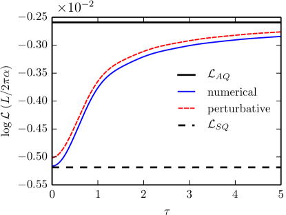
Figure 4: Plot for $\log\mathcal{L}(t)$, in units of $L/(2\pi\alpha)$, in the large time (asymptotic) limit as a function of $\tau$. Here we have chosen $t=\tau+50$, and $\delta_{g}/v_{i}=0.1$ for an initial choice of $g_{i}/v_{i}=0.1$. The solid (blue) line denotes the exact numerical result and the dashed(red) lines shows the perturbative solution. The solid (dashed) horizontal line is the analytical expression for the LE in the adiabatic (sudden) quench limit for $t\to\infty$.

For small $\tau$, incorporating correction to the lowest order in $\tau$ appearing in Eq.(36), we find

$$\mathcal{L}_{SQ^{+}}(t\to\infty)\approx\text{exp}\left[-\frac{L}{2\pi\alpha}\frac{\delta_{g}^{2}v_{0}^{2}}{2v_{i}^{4}}\left\{1-\frac{v_{i}^{2}\tau^{2}}{18\alpha^{2}}\right\}\right];$$ (37)

where the sudden quench result [Eq.(31)] is recovered for $\tau=0$. This is to be noted that the lowest order correction term (over the $\tau=0$ case) scales as $\tau^{2}$ which can be be understood physically using a simple quantum mechanical argument. The system changes over a time scale of $\tau$, and the time evolved wave function can be obtained by integrating the Schrödinger equation within the interval $[0,\tau]$:

$$|\psi(\tau)\rangle-|\psi(0)\rangle=-\frac{i}{\hbar}\int_{0}^{\tau}H(t)~{}dt~{}.$$ (38)

Since the integrand is finite, the integral is of the order of $\tau$ [see Ref. shankar, ]. We therefore get a correction which varies as $\tau^{2}$, in the probability of excitation to the $n$-th excited state, which is given by $P_{n}=|\langle\psi_{0}|\psi_{n}\rangle|^{2}$. Here $|{\psi_{0}}\rangle$ is the initial ground state and $|{\psi_{n}}\rangle$ is the $n$-th excited state associated with the final time evolved Hamiltonian. This correction scaling as $\tau^{2}$ appears in the LE when LM is being quenched with a small but finite $\tau$.

In the limit of large $\tau$, the LE in the asymptotic limit is obtained by retaining only lowest order term (of the order $1/\tau$) in Eq.(36); this is given by

$$\mathcal{L}_{AQ^{-}}(t\to\infty)\approx\text{exp}\left[-\frac{L}{2\pi\alpha}\frac{\delta_{g}^{2}v_{0}^{2}}{4v_{i}^{4}}\left\{1+\frac{\pi\alpha}{2\tau v_{i}}\right\}\right].$$ (39)

The second term of Eq.(39) represents the first order correction in $\tau$ over the adiabatic quench ($\tau=\infty$ limit). We emphasise that the correction to the LE over the adiabatic limit for $t\to\infty$ scales as $1/\tau$ .

This can be understood by the following argument Grandi . Lets assume a parameter $\lambda$ of a $d$-dimensional Hamiltonian is driven as $\lambda(t)=t/\tau$ within the gapless phase with quasiparticle energy dispersion as $\epsilon_{q}\sim A(\lambda)q^{z}$, where $z$ is the dynamical critical exponent. When the dynamics is adiabatic, the excitation to higher energy state becomes suppressed when the rate of change of $\lambda$ is small compared to the internal time scale, i. e., $\dot{\epsilon}_{q}(\lambda)/\epsilon_{q}(\lambda)\ll\epsilon_{q}(\lambda)$. For the present model, the inherent time scale is given by $L/v_{i}$ while the external time scale is $\tau$. Adiabaticity breaks down when $\dot{\epsilon}_{q}(\lambda)\sim\epsilon_{q}^{2}(\lambda)$. This leads to a characteristic momentum scale which is related to the quench rate $\tau$ through the following relation:

$$\tilde{q}^{z}\sim\frac{1}{\tau A(\lambda)}\frac{\delta{\ln A(\lambda)}}{\delta\lambda}.$$ (40)

The total number of quasiparticle excitation to higher state is proportional to the phase space volume ${\tilde{q}}^{d}\sim\tau^{-d/z}$. This scaling law holds true for $d/z\leq 2$. In the present model, therefore the measure of the defect density given by $|h(q,t)|^{2}$ integrated over all momenta mode scales as $1/\tau$; this scaling is reflected in the asymptotic behaviour of the LE.

One can observe that $\mathcal{L}^{SQ}_{t\to\infty}=(\mathcal{L}^{AQ}_{t\to\infty})^{2}$ with the proper adiabatic and sudden limits of $\tau$ i.e., $\tau=\infty$ for perfect adiabatic quenching and $\tau=0$ for perfect sudden quenching. But when LM is being quenched through a finite driving rate $1/\tau$, the infinite time expressions of LE, for a fast and a slow quenching scheme, is modified in a relevant way. The ground state conjecture does not hold true for a finite $\tau$. The LE in the slow quenching case could not be described as an modulo square overlap between initial and final ground state of LM. The finite $\tau$ brings additional contributions coming from higher excited state to the infinite time LE. In the infinite time limit LE under a fast quenching scheme is also modified from the $\tau=0$ limit of LE.

VI conclusion

In this manuscript, we have studied the dynamics of a Luttinger model following an interaction quench when the quench is applied over a finite duration $\tau$. The Loschmidt echo for a finite time linear interaction quench is studied in both large $\tau$ and small $\tau$ limits. In particular, we reproduce the results for the adiabatic and sudden quench limits derived earlier Dora_prl13 , and using perturbative solutions we estimate the corrections to both these limiting situations in the early time limit as well as the infinite time limit. We also compare the perturbative results with the exact numerical ones, and obtain a reasonably good agreement between them.

Let us summarize the interesting findings of our study: we find that the correction terms scales as $1/\tau$ in the large $\tau$ limit and as $\tau^{2}$ in the $\tau\to 0$ limit which show up both in the early time and the large time behaviour. We propose generic scaling relations to justify the scaling of the correction terms. Finally, our results confirm that for a finite $\tau$ the excited states contribute non-trivially to the echo even in the asymptotic limit ($t\to\infty$).

Note that our results [see for e.g., Eqs. (LABEL:LEexp1)-(39)] depend on the non-universal short distance cutoff, $\alpha$. This may be a consequence of the fact that we are using a linear ramp, whose derivative has discontinuities at $t=0$ and $t=\tau$. A Fourier transform of such a non-analytic ramp has a fat high frequency tail, which is governed by a power law DzairmagaPRB2011 . The high frequencies in the tail give rise to excitations that are beyond the low-energy description of the Luttinger model. We believe that if the linear ramp were replaced by a smooth quench protocol [e.g., $\tanh(t/\tau)$-like], then the tail would be exponential and the inverse ultraviolet cutoff $\alpha$ would not appear in the results .

Finally we note that the Luttinger model uses a linearized dispersion relation which is valid only in a small window of energy around the Fermi points. In any realistic quenching scenario, the system will be excited to energies where, the non-linearities of the dispersion relation begin to play a role in the dynamics via the so called ‘umklapp’ scattering of the right- and left-moving modes. It is commonly argued in the literature that all these deviations are irrelevant in the renormalization group sense, which means that their effects are limited, or that their effects die out if we wait for long enough times. Another way to avoid exciting the system to very high energies (where the Luttinger model is not valid), is to tune the interaction parameter ($g$) in a regime which is much smaller than the Fermi energy of the system cazalila_prl06 . However, it is not completely clear, if the Luttinger model is appropriate to describe the quench dynamics in a realistic physical system, even though we believe that the long-term dynamics of the system should be dominated by the low-energy excitations.

- (1) A. Polkovnikov, K. Sengupta, A. Silva, and M. Vengalattore, Rev. Mod. Phys. 83, 863 (2011).
- (2) A. Dutta, , arXiv:1012.0653 (2010).
- (3) J. Dziarmaga, Adv. Phys. 59, 1063 (2010).
- (4) S. Sachdev, Quantum Phase Transitions (Cambridge University Press, Cambridge, England,1999).
- (5) I. Bloch, J. Dalibard, and W. Zwerger, Rev. Mod. Phys. 80, 885 (2008).
- (6) S. Hofferberth, I. Lesanovsky, B. Fischer, T. Schumm, and J. Schmiedmayer, Nature 449, 324-327 ( 2007).
- (7) Asher Peres, Phys. Rev. A30, 1610 (1984).
- (8) A. Goussev, R. A. Jalabert, H. M. Pastawski, and D. A. Wisniacki, Scholarpedia 7, 11 687 (2012).
- (9) F. Pollmann, S. Mukerjee, A. G. Green, and J. E. Moore, Phys. Rev. E 81, 020101(R) (2010).
- (10) M. Heyl, A. Polkovnikov, and S. Kehrein, Phys. Rev. Lett., 110, 135704 (2013). C. Karrasch and D. Schuricht, Phys. Rev. B 87, 195104 (2013).
- (11) H. T. Quan, Z. Song, X. F. Liu, P. Zanardi, and C. P. Sun, Phys. Rev. Lett. 96, 140604 (2006).
- (12) S. Sharma, V. Mukherjee, and A. Dutta, Eur. Phys. JB, 85, 143 (2012).
- (13) D. Rossini, T. Calarco, V. Giovannetti, S. Montangero, and R. Fazio, Phys. Rev. A75, 032333 (2007).
- (14) J. Zhang et. al. ,Phys. Rev. A 79, 012305 (2009). Michael Knap et. al., Phys. Rev. X 2, 041020 (2012).
- (15) A. Silva, Phys. Rev. Lett., 101, 120603 (2008).
- (16) B. Damski, H. T. Quan, and W. H. Zurek, Phys. Rev. A 83, 062104 (2011).
- (17) L. CamposVenuti, and Paolo Zanardi, Phys. Rev. A, 81, 022113 (2010). L. CamposVenuti, N. T. Jacobson, S. Santra, and P. Zanardi, Phys. Rev. Lett. 107, 010403 (2011).
- (18) B. Damski, H. T. Quan, and W. H. Zurek, Phys. Rev. A 83, 062104 (2011).
- (19) T. Nag, U. Divakaran, and A. Dutta, Phys. Rev. B 86, 020401 (R) (2012). V. Mukherjee, S. Sharma, and A. Dutta, Phys. Rev. B 86, 020301 (R) (2012).
- (20) M.A. Cazalilla, Phys. Rev. Lett. 97, 156403 (2006).
- (21) E. Perfetto, and G. Stefanucci, Europhys. Lett. 95, 10006 (2011).
- (22) B. Dóra, M. Haque, and G. Zárand, Phys. Rev. Lett. 106, 156406 (2011).
- (23) B. Dóra, F. Pollmann, J. Fortágh, and G. Zárand, Phys. Rev. Lett. 111, 046402 (2013).
- (24) F. Pollmann, M. Haque, and B. Dóra, Phys. Rev. B 87, 041109(R) (2013).
- (25) J. Rentrop, D. Schuricht, and V. Meden, New J. Phys. 14, 075001 (2012).
- (26) C. Karrasch, J. Rentrop, D. Schuricht and V. Meden, Phys. Rev. Lett. 109, 126406 (2012). E. Coira, F. Becca, and A. Parola, European Physical Journal B 86, 55 (2013).
- (27) T. Giamarchi, Quantum Physics in One Dimension, Oxford University, Oxford, 2004. S. Rao and D. Sen, in Field Theories in Condensed Matter Physics, edited by S. Rao, Hindustan Book Agency, New Delhi, 2001). A. O. Gogolin, A. A. Nersesyan, and A. M. Tsvelik, Bosonization and Strongly Correlated Systems, Cambridge University Press, Cambridge, 1998.
- (28) M. A. Cazalilla, R. Citro, T. Giamarchi, E. Orignac, and M. Rigol, Rev. Mod. Phys. 83, 1405 (2011).
- (29) D. Chen, M. White, C. Borries, and B. DeMarco, Phys. Rev. Lett. 106, 235304 (2011).
- (30) B. Dóra, Á. Bácsi, and G. Zárand, Phys. Rev. B86, 161109 (R) (2012).
- (31) J. Dziarmaga, and M. Tylutki, Phys. Rev. B 84, 214522 (2011).
- (32) A. Iucci, and M. A. Cazalilla, Phys. Rev. A80, 063619 (2009).
- (33) A. Mitra, and T. Giamarchi, Phys. Rev. Lett. 107, 150602 (2011).
- (34) A. Mitra, Phys. Rev. Lett. 109, 260601 (2012); Phys. Rev. B 87, 205109 (2013).
- (35) J. Sirker, Phys. Rev. Lett. 105, 117203 (2010).
- (36) M.-F. Yang, Phys. Rev. B76, 180403 (R) (2007). J. O. Fjaerstad, J. Stat. Mech. (2008), P07011.
- (37) M. Heyl, and M. Vojta, arXiv:1310.6226.
- (38) R. Shankar, Principles of Quantum Mechanics (Second Edition, Springer, 1994).
- (39) C. De Grandi and A. Polkovnikov in Quantum Quenching, Annealing and Computation, edited by A. Das, A. Chandra and B. K. Chakrabarti, Lect. Notes in Phys., vol. 802 (Springer, Heidelberg 2010).