Heterogeneous Delays in Neural Networks

Abstract

We investigate heterogeneous coupling delays in complex networks of excitable elements described by the FitzHugh-Nagumo model. The effects of discrete as well as of uni- and bimodal continuous distributions are studied with a focus on different topologies, i.e., regular, small-world, and random networks. In the case of two discrete delay times resonance effects play a major role: Depending on the ratio of the delay times, various characteristic spiking scenarios, such as coherent or asynchronous spiking, arise. For continuous delay distributions different dynamical patterns emerge depending on the width of the distribution. For small distribution widths, we find highly synchronized spiking, while for intermediate widths only spiking with low degree of synchrony persists, which is associated with traveling disruptions, partial amplitude death, or subnetwork synchronization, depending sensitively on the network topology. If the inhomogeneity of the coupling delays becomes too large, global amplitude death is induced.

1 Introduction

Over the past decades the study of networks has gained increasing importance due to its widespread applicability such as in social sciences, computer science, economics, biology, physiology, and ecology. In the context of dynamics on networks, synchronization is a field of high interest PIK01 . It is an important phenomenon, for instance, in neuroscience ROE97 ; POE01 ; ROS05 ; SIN07 ; VIC08 ; MAS08 ; LEH11 ; KAN11a ; PER11a ; KEA12 . The master stability function is a powerful tool to investigate the stability of zero-lag, cluster and group synchronization PEC98 ; KES07 ; SOR07 ; DAH12 but generally is limited to networks of identical systems with one discrete delay time. Only under the condition of commuting coupling matrices, two or more discrete delay times can be considered SOR07 ; DAH12 . However, real-world networks are not limited to cases well described by commuting coupling matrices and discrete delay times but are often characterized by a complex topology, for example of random or small-world type, and heterogeneous delays. In the brain, the length, the diameter, and the kind of the axons between the neurons determine the nerve conduction velocity. Therefore the propagation speed between neurons can vary between $1$ and $100$ mm/ms KOC99 . The aim of this paper is to investigate synchronization and other space-time patterns in the presence of heterogeneous delay times. In particular we consider two discrete delay times as well as unimodal and bimodal delay distributions. In the context of the brain, a bimodal distribution is a good first approximation if coupling on two different length scales is considered, i.e., nearby connections within brain areas associated with short delays, and links between distant areas characterized by long delays.

The paper is organized as follows: In Sec. 2 we introduce the neural model and the delay coupling. Section 3 discusses possible spiking scenarios in regular, small-world, and random networks if the coupling delays are drawn from a unimodal distributions. In Sec. 4, we explore the role of resonance effects in the presence of two different discrete delay times. Section 5 extends the results of Secs. 2 and 3 by investigating a bimodal delay distribution. A conclusion is given in Sec. 6.

2 Model

The local dynamics of each node in the network is modeled by the FitzHugh-Nagumo differential equations FIT61 ; NAG62 . The FitzHugh-Nagumo model is paradigmatic for excitable dynamics close to a Hopf bifurcation LIN04 , which is not only characteristic for neurons but also occurs in the context of other systems ranging from electronic circuits HEI10 to cardiovascular tissues and the climate system MUR93 ; IZH00a . Each node of the network is described as follows:

$$\varepsilon\dot{u}_{i} =u_{i}-\frac{u_{i}^{3}}{3}-v_{i}+C\sum_{j=1}^{N}G_{ij}\left[u_{j}(t-\tau_{ij})-u_{i}(t)\right],$$

$$\dot{v}_{i} =u_{i}+a,\quad i=1,\ldots,N,$$ (1)

where $u_{i}$ and $v_{i}$ denote the activator and inhibitor variable of the nodes $i=1,\ldots,N$, respectively, and $\varepsilon$ is a time-scale parameter and typically small (here we will use $\varepsilon=0.01$), meaning that $u_{i}$ becomes a fast variable while $v_{i}$ changes slowly. In the uncoupled system ($C=0$), $a$ is the threshold parameter: For $a>1$ the system is excitable while for $a<1$ it exhibits self-sustained periodic firing. This is due to a supercritical Hopf bifurcation at $a=1$ with a locally stable fixed point for $a>1$ and a stable limit cycle for $a<1$. We choose $a=1.3$ such that the system operates in the excitable regime.

The coupling matrix $\textbf{G}=\{G_{ij}\}$ defines which nodes are connected to each other. An invariant synchronization manifold will only exist if G has a constant row sum; without loss of generality we assume the row sum to be unity, i.e., $\sum_{j}G_{ij}=1$, $i=1,\ldots,N$. We construct the matrix G by setting the entry $G_{ij}$ equal to 1 (0) if the $j$th node couples (does not couple) into the $i$th node. After repeating this procedure for all entries of $G_{ij}$, we normalize each row to unity. The overall coupling strength is given by $C$. Throughout the paper, we use bidirectional coupling, which means that signals can always be transmitted in both directions. This makes G a symmetric matrix (before we normalize each row sum to $1$). $\textbf{T}=\{\tau_{ij}\}$ is the delay matrix, i.e., $\tau_{ij}$ is the time the signal needs to propagate from the $j$th to the $i$th node.

3 Unimodal delay distributions in complex networks

The first step in going from one discrete delay time to more realistic models with heterogeneous delay times is to consider a unimodal distribution. In the following, we choose the elements of the delay matrix T randomly from a normal distribution $\mathcal{N}(\tau_{\mu},\sigma^{2})$ with mean $\tau_{\mu}$ and standard deviation $\sigma$.

In Ref. LEH11 , system (1) with a $\delta$-distribution of the delay times was investigated. For excitatory coupling – i.e., all entries of G are positive – it was shown that synchronized spiking with an inter-spike interval (ISI) of $\tau_{\mu}$ is always stable independently of coupling strength and delay time (as long as both are large enough to induce any spiking at all). In this Section, we will discuss how robust these results are if we increase $\sigma$. In particular we will focus on the effect of the underlying topology – regular, small-world, or random – on the dynamics. These topologies are constructed as follows: In a regular ring network each node is connected with equal strength to its $k$ nearest neighbors to the left and to the right, i.e., the node degree is $2k$. If additional excitatory links are added with a probability $p$ to such a regular network, a small-world network arises WAT98 ; MON99 ; NEW99b . In a random network each node is linked with probability $p$ to every other node RAP57 ; SOL51 ; ERD59 ; ERD60 .

Depending on the distribution width, the topology, and initial conditions there are essentially three different types of dynamics observable: Highly-synchronous spiking, spiking, and global amplitude death, from which the spiking can be subdivided into several subclasses.

3.1 Spiking patterns and amplitude death

Highly-synchronous spiking

If $\sigma$ is small enough, stable synchronization with an ISI of $\tau_{\mu}$ will persist, while the spikes will be broader than for a delta distribution.

The quality of synchronization can be measured using the Kuramoto order parameter KUR84 :

$$R=\frac{1}{N_{s}}\left|\sum_{j=1}^{N_{s}}e^{i\phi_{j}}\right|,$$ (2)

where $N_{s}$ is the number of spiking nodes. In other words, we do not include non-spiking nodes when calculating the Kuramoto order parameter. $\phi_{j}$ is the phase of the $j$th oscillator. $\phi_{j}$ can be defined as

$$\phi_{j}=2\pi\frac{t-t_{n}}{t_{n}-t_{n-1}},$$ (3)

where $t_{n}$ is the time of the last spike of the $j$th neurons ROS01 . For $R=1$, perfect phase synchronization is reached; if $R\approx 0$, the network is desynchronized. We consider a network as highly synchronized if $R>0.99$ after all transient effects have vanished.

Spiking

For intermediate $\sigma$, different dynamical subclasses can be observed where the network still exhibits spikes, but not necessarily in a highly synchronized manner: approximate synchronization, traveling disruptions, and partial amplitude death.

The first scenario is that all nodes in the network still synchronize but because of the non-zero width of the delay distribution the incoming spikes do not arrive exactly at the same time but with some slight deviations. Thus, $R$ drops below $0.99$, i.e., the network is not any longer highly synchronized. Figure 1(a) shows as an example the time series of approximate synchronization: The spike times are marked by red dots in panel (a) and the Kuramoto order parameter $R(t)$ is plotted in panel (b). After some transienst time the spikes synchronize fast. However, $R$ remains below $0.99$.

\begin{overpic}[width=433.62pt]{fig1.png} \put(0.0,36.0){(a)} \put(0.0,13.0){(b)} \end{overpic}

Figure 1: (a) Approximately synchronized spiking pattern (red dots) and (b) order parameter $R$ (blue line) vs time for a small-world network with a delay distribution with standard deviation $\sigma=0.2$. Parameters: $N=50$, $p=0.51$, $k=2$, $C=1.0$, $a=1.3$, $\varepsilon=0.01$ and $\tau_{\mu}=5$. The initial condition is $u_{i}=-a$, $v_{i}=a-a^{3}/3$ for all $i=1,...,50$. The history function of all nodes is the spiking state.

A fairly well synchronized behavior is the most common spiking pattern, but in regular-ring structures as well as in some small-world realizations a different type of behavior can be observed as well: In Fig. 2(a) disruption travels along many nodes in a ring network without causing amplitude death to the network. Such traveling disruptions can arise for fairly high standard deviations, e.g., in Fig. 2, $\sigma=0.2$, however, the probability for this behavior is quite low since amplitude death is much more common as will be discussed later.

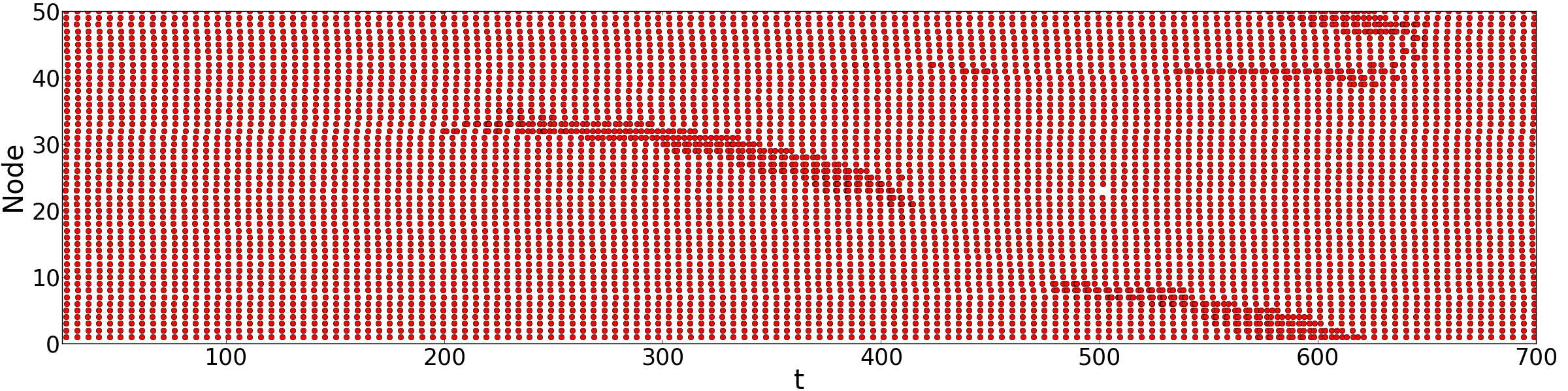
Figure 2: Spiking patterns showing traveling disruptions in a regular ring network with $N=50$ nodes and $\sigma=0.2$. Red dots indicate spikes. Other parameters as in Fig. 1.

Furthermore, networks can be observed where only a subset of nodes spikes, while the other nodes undergo partial amplitude death. This is the case if, by chance, in a fairly isolated subnetwork the deviation of delay times is smaller than the deviation in the whole network. In large random networks the probability for this is small, since fairly isolated subnetworks arise rarely as they require some kind of ordered structure in the network. In case of small-world networks though, it is more likely that a subnetwork can maintain stably synchronized spiking while other regions of the network undergo amplitude death. This scenario is depicted in Fig. 3. One can also observe cases where a part of the network stops spiking temporarily but then gets excited again and fires synchroneously with the rest of the network. This reanimation is also observable in Fig. 3 around node no. 43.

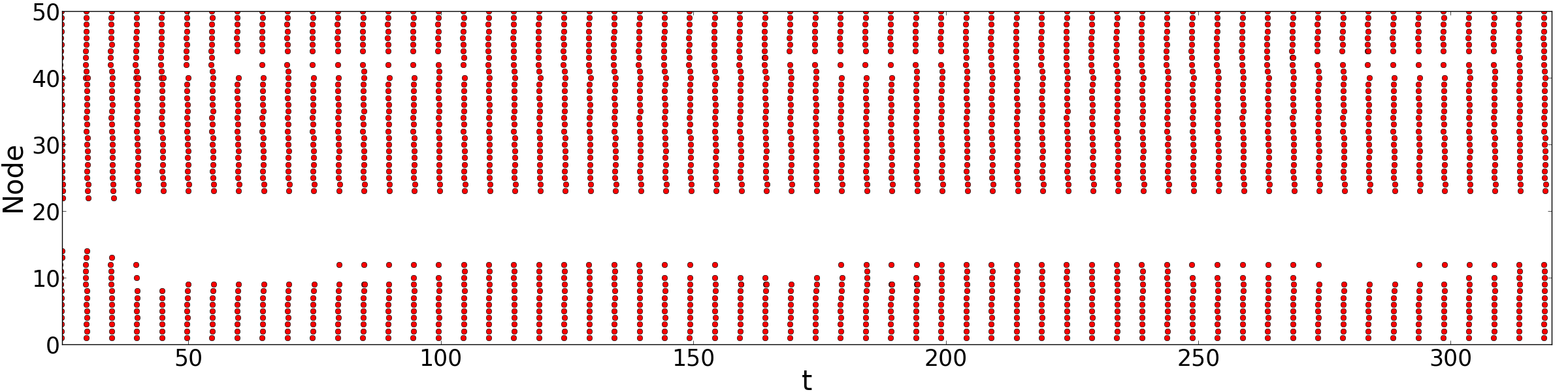
Figure 3: Spiking pattern showing partial amplitude death in a small-world network ($N=50$, $p=0.51$) for a delay distribution with standard deviation of $\sigma=0.12$. Red dots mark spikes. Other parameters as in Fig. 1.

Global Amplitude death

If $\sigma$ becomes too large, amplitude death is induced, i.e., all nodes remain in the fixed point and no spikes are released.

Amplitude death is caused by two different factors. First, each node needs excitation from many neighbors at the same time. As $\sigma$ increases, the probability that enough spikes from the neighboring neurons arrive sufficiently close in time decreases. Furthermore, the nodes’ neighbors which spike too early or too late and which are therefore already or still in the fixed point $(u_{*},v_{*})$ will pull the node back as they give rise to a negative coupling term of the form $u_{*}-u_{i}$ in Eq. (1), where we considered the effect on the $i$th node.

Second, even if a spike can be excited by the arriving spikes, for large $\sigma$ retarded spikes are likely to perturb the trajectory of the already spiking node. The result is a spike with a low amplitude, which will be fed back into the network. If this happens on a global scale, i.e., if there is no fairly isolated subnetwork, which can maintain the amplitude of the spikes, the spikes will be damped in the course of time and will eventually lead to global amplitude death.

\begin{overpic}[width=216.81pt]{fig4.png} \put(12.5,72.0){(a)} \put(12.5,50.0){(b)} \end{overpic}

Figure 4: (a) Time series of $u$ (red solid) and $v$ (blue dotted), and (b) phase space of a single node undergoing amplitude death. The node is part of a small-world network ($N=50$, $p=0.51$) with $\sigma=0.15$. (b) Trajectory (red solid) and $u$-nullcline (blue dashed). Other parameters as in Fig. 1.

Both of the mentioned effects can be seen in the trajectory depicted in Fig. 4. The first effect prevents the trajectory to reach the far right nullcline (dashed blue) in the phase space, which would have been reached in the absence of the negative force pulling it to the left. The second effect causes the trajectory to wiggle around on its round trip, instead of allowing a smooth course. This is due to excitations arriving during the round trip which pull the trajectory back and forth. Both effects lead to an decreasing amplitude and eventually to amplitude death.

3.2 Statistical analysis

Which kind of dynamics will take place on a network depends on the topology, the width of the delay distribution, and on initial conditions. For a systematic study, we calculate $p_{s}(\sigma)$ and $p_{h}(\sigma)$, where $p_{s}(\sigma)$ and $p_{h}(\sigma)$ are the probabilities that for a given realization of the delay matrix $\mathbf{T}$ with the standard deviation $\sigma$ and a given realization of the network topology, the network shows any kind of spiking behavior ($p_{s}$) or highly synchronized spiking ($p_{h}$), respectively. Note that $p_{h}\leq p_{s}$ as the highly synchronized networks are a subset of the spiking ones. Figure 5 shows $p_{h}(\sigma)$ (dotted lines) and $p_{s}(\sigma)$ (solid lines) for (a) a regular ring, (b) a small-world network, and (c) a random network.

\begin{overpic}[width=433.62pt]{fig5.png} \put(11.0,68.0){(a)} \put(11.0,46.0){(b)} \put(11.0,23.0){(c)} \end{overpic}

Figure 5: Probability of spiking $p_{s}$ (solid lines) and of highly synchronized spiking $p_{h}$ (dotted lines) vs standard deviation of delay distribution $\sigma$ for (a) a regular ring networks with $k=2$, i.e, each node is connected to its nearest and next-nearest neigbor to the left and to the right, (b) small-world networks with $k=2$ and $p=0.51$ and (c) random networks with $p=0.51$ and different network sizes $N=20$ (blue), $N=50$ (red), $N=100$ (green). Other parameters as in Fig. 1.

\begin{overpic}[width=433.62pt]{fig6.png} \put(0.0,74.0){(a)} \put(0.0,61.2){(b)} \put(0.0,49.0){(c)} \put(0.0,36.2){(d)} \put(0.0,24.0){(e)} \put(0.0,11.2){(f)} \end{overpic}

Figure 6: Spiking patterns showing subnetwork synchronization in a regular ring network with $N=50$ nodes for different $\sigma$: (a)-(d) $\sigma=0.1$; (e),(f)$\sigma=0.13$. Panel (a),(c),(e): Red dots indicate spikes; Panel (b),(d),(f): Kuramoto order parameter $R$. Note that (c),(d) show the same simulation as (a),(b) for a longer time series. Other parameters as in Fig. 1.

Figure 5 reveals that for each type of topology, a threshold value $\sigma_{t}$ exists above which global amplitude death almost certainly sets in, i.e., $p_{s}(\sigma)\approx 0$ for $\sigma>\sigma_{t}$ (see solid lines in Fig. 5). Comparing the different topologies, it is interesting to note that $\sigma_{t}$ is smaller, about 0.15 for $N=100$, in the case of the small-world and the random network as compared to the regular network, where $\sigma_{t}$ is about 0.2. Furthermore, in small-world and random networks $\sigma_{t}$ is preceded by a steep sigmoidal transition, while in the case of the regular network the transition is less steep and characterized by a long tail making it difficult to clearly define $\sigma_{t}$. As discussed later in detail, the reason for this behavior is that in regular networks often spiking subnetworks survive, which is very unlikely for small world and random networks. Noteworthy is also that in the case of regular networks global amplitude death occurs later for larger networks, while in small-world and random networks small networks survive longer.

The topology of the network is even more critical when considering the fraction of highly synchronized networks, i.e., the curves for $p_{h}$ (dashed lines in Fig. 5). A particularly interesting phenomenon is the non-monotonic behavior of $p_{h}$ in the regular ring networks (Fig. 5(a) dashed). While the fraction of highly synchronized networks rapidly drops for small $\sigma$, it rises again as the fraction of spiking networks falls. For large $\sigma$, $p_{h}$ and $p_{s}$ converge, i.e., only highly synchronized networks survive for higher $\sigma$. This is certainly not the case for intermediate $\sigma$, where most of the surviving networks are not highly-synchronized. This counterintuitive behavior of $p_{h}$ can be explained by the fact that for intermediate $\sigma$ the network splits into subnetworks as shown in Fig. 6: Panel (a) shows the spiking pattern of a regular ring for intermediate $\sigma$ ( $\sigma=0.1$), i.e., a value for which almost all networks are spiking in a highly asynchronous manner; Panel (b) depicts the corresponding Kuramoto order parameter $R$. Panels (c) and (d) show the same for a longer time series up to $t=2000$. It can be clearly seen that after some transient time ($t\approx 500$), the network consists of two different subnetworks, at times separated by a patch of partial amplitude death (subnetwork synchronization). Simulations indicate that these subnetworks survive for infinitely long times and do not synchronize. As a consequence the two networks have slightly different ISIs resulting in a beating behavior: For a while the networks are almost synchronized, then their spiking times drift apart leading to slow oscillations in the Kuramoto order parameter. Thus, most of the times $R$ is much smaller than $0.99$ and the networks is not classified as highly synchronized.

If $\sigma$ is increased above approximately $0.13$, the system either exhibits global amplitude death, or the spiking in one of the subnetworks only dies out. The nodes in the surviving subnetwork remain highly synchronized, since they all interact and the distribution width is not yet too large. Thus almost all networks which do not undergo global amplitude death are highly synchronized (recall that in the definition Eq. (2) of the order parameter only spiking nodes are considered). For even larger $\sigma$, global amplitude death can be observed in almost all network realizations.

In contrast, in small-world networks a different behavior can be observed: $p_{s}$ and $p_{h}$ do not coincide for large $\sigma$ but the spiking networks survive longer than the highly synchronized networks (see Fig. 5(b)). The reason is that in a small-world network subnetworks do not easily arise because the additional long range links connect the different parts of the network. However, more and more disruptions occur for larger $\sigma$. They decrease $R$ and are thus responsible for the fact that less highly synchronized network persist.

Neither traveling disruptions nor partial amplitude death can be observed in a random network. Therefore, almost all surviving networks are highly synchronized, as shown in Fig. 5(c).

4 Two discrete delay times

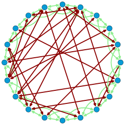
Figure 7: Example of a small-world network, where inner connections (red (black) arrows) have a delay $\tau_{1}$, while the outer connections of the underlying regular ring (green (gray) arrows) are characterized by a delay $\tau_{2}$.

\begin{overpic}[width=433.62pt]{fig8a.png} \put(4.0,14.0){(a)} \end{overpic}

\begin{overpic}[width=433.62pt]{fig8b.png} \put(4.0,14.0){(b)} \end{overpic}

Figure 8: Interspike intervals (ISIs) in a small-world network plotted versus the delay $\tau_{1}$ of the inner connections. (a) Simulations. (b) Mathematical reconstruction according to Eq. (4). $\tau_{2}=6$, $N=20$, $k=2$, $p=0.51$. Other parameters as in Fig. 1.

In Ref. SCH08 ; PAN12 it was shown that already in a simple motif of two coupled FitzHugh-Nagumo systems with two or three different delay times, complex dynamics arise. In particular, resonance effects between the different delay times proved to be crucial. Here we study the effect of two discrete delay times in larger complex networks. We focus on small-world networks (see Fig. 7 for a schematic diagram) and separate the two parts of the network in a meaningful way by choosing $\tau_{2}$ as the delay associated with the underlying regular network (green (gray) arrows), and $\tau_{1}$ as the delay time of the additional random links (red (black) arrows).

Depending on the ratio between $\tau_{1}$ and $\tau_{2}$, different spiking patterns emerge. We measure the ISIs (Interspike intervals) in simulations while gradually increasing $\tau_{1}$ for fixed $\tau_{2}=6$ as depicted in Fig. 8(a). Figure 8(b) shows a mathematical reconstruction of the results obtained numerically in panel (a) based on the following argument: Any spike in the network will eventually be fed into the system again with a delay. Starting from the synchronous manifold, i.e., $(u_{1},v_{1})=\ldots=(u_{N},v_{N})\equiv(u_{s},v_{s})$, spikes will first reappear with a delay of either $\tau_{1}$ or $\tau_{2}$. Those spikes again will be transmitted to other neurons with one of the two delays meaning that eventually nearly all possible combinations of forwarding a spike with either delay $\tau_{1}$ or $\tau_{2}$ will be observable in the network. Thus, we can obtain all possible spiking times from the expression:

$$T_{lk}=l\tau_{1}+k\tau_{2}$$ (4)

with $l,k\in\mathbb{N}_{0}$.

After sorting all possible $T_{lk}$ by size, the ISIs are given by the difference between neighboring elements in the sorted list. Note that for the mathematical reconstruction in Fig. 8(b), ISIs $<0.1$ were discarded since the spikes have a width of approximately 0.1 if they are close, i.e., the ISI is small.

Coherent spiking, i.e., spiking with a constant ISI, is observable as a result of resonance effects: For a case where the ratio of the multiple delay times is given by

$$n\tau_{1}=m\tau_{2}$$ (5)

with $m,n\in\mathbb{N}$, coherent spiking with an ISI equal to

$$\frac{\tau_{1}}{m}=\frac{\tau_{2}}{n}$$ (6)

is induced, where we choose the smallest possible $m$ and $n$, i.e., $m$ and $n$ do not have common divisors. A similar relation has been obtained in Ref. ZIG09 for a system of two time-discrete systems with several unequal delays and in Ref. PAN12 for a system of two coupled FitzHugh-Nagumo systems with unequal coupling and self-feedback delay times. Note that $n$ and $m$ in Eq. (5) cannot be chosen arbitrarily large: If $\tau_{1}/m$ or $\tau_{2}/n$ is smaller than 0.4 spikes run into each other and coherent spiking is not possible any longer.

5 Bimodal delay distributions

In this Section, we discuss a network characterized by a bimodal delay distribution. In such a network, the superposition of two normal distributions with two mean delay times $\tau_{\mu}^{(1)}$ and $\tau_{\mu}^{(2)}$ and two standard deviations $\sigma^{(1)}$ and $\sigma^{(2)}$ determines the delay between nodes.

Peak distance of the distribution

To study the effects of different bimodal distributions, we start by changing the difference $\tau_{\mu}^{(1)}-\tau_{\mu}^{(2)}$ between the two peaks of the distribution, while keeping the standard deviations constant: $\sigma^{(1)}=\sigma^{(2)}=0.01$. The result is shown in Fig. 9, where the ISIs are depicted vs $\tau_{\mu}^{(1)}-\tau_{\mu}^{(2)}$.

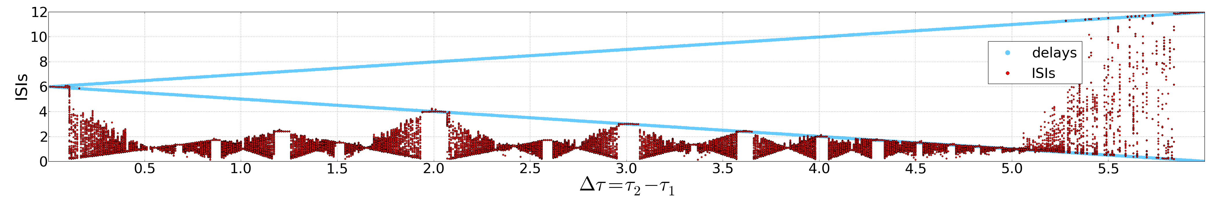
Figure 9: Interspike intervals (ISIs) (red dots) and delays (blue dots) of a small-world network. $N=50$, $\sigma^{(1)}=\sigma^{(2)}=\sigma=0.01$, $p=0.51$. Other parameters as in Fig. 1.

Figure 9 shows that for distributions with small and medium width, i.e., $\sigma^{(1)}=\sigma^{(2)}<0.01$, the ISIs follow the condition of Eq. (5) discussed for the case of two discrete delay times if we substitute $\tau_{1}$ and $\tau_{2}$ by the two peak positions, i.e., $\tau_{1}=\tau_{\mu}^{(1)}$ and $\tau_{2}=\tau_{\mu}^{(2)}$. The same pattern also emerges for random networks (not shown here).

Width of the distribution

If the width of the two peaks becomes too large, Eqs. (5) and (6) fail as good descriptions for the spike times and ISIs. Figure 10 depicts the ISIs as function of the peak widths $\sigma^{(1)}=\sigma^{(2)}\equiv\sigma$ for (a) a small world network with $\tau_{\mu}^{(1)}=6$ and $\tau_{\mu}^{(2)}=8$, (b) a small world network with $\tau_{\mu}^{(1)}=5$ and $\tau_{\mu}^{(2)}=10$, and (c) a regular ring with $\tau_{\mu}^{(1)}=6$ and $\tau_{\mu}^{(2)}=8$. For small $\sigma$ ($\sigma<0.05$ in (a), $\sigma<0.09$ in (b), and $\sigma<0.03$ in (c)) the ISIs can be found by evaluating Eq. (6): For the combination $\tau_{\mu}^{(1)}=6$ and $\tau_{\mu}^{(2)}=8$, we find coherent spiking with an ISI of 2, for $\tau_{\mu}^{(1)}=5$ and $\tau_{\mu}^{(2)}=10$ the ISI is 5.

As $\sigma$ increases, the coherent spiking breaks down. Instead, networks can be observed where different parts of the network spike with different ISIs. This effect is particularly prominent in the case of a ring network, since in such a network isolated subnetworks can easily arise, in which the delay distribution allows for persistent spiking. Figure 11 shows exemplarily the dynamics in a regular ring network for intermediate values of the distribution width ($\sigma=0.05$ in panels (a),(b),(c), $\sigma=0.08$ in panels (d),(e),(f)). Panels (c) and (f) show the spiking patterns. For the lower $\sigma$ value, (panel (c)), a part of the network (from about node 30 to node 45) exhibits partial amplitude death, while the majority of the nodes keeps spiking though in different subnetworks characterized by different ISIs. For the higher value of $\sigma$, only a small subset of spiking nodes persists. The time series of node 0 in panel (a) and its phase portrait in (b) show that no longer all spikes have the same amplitude, but the amplitudes vary slightly in an irregular fashion due to the coupling with other nodes with inhomogeneous delay times.

If $\sigma$ is further increased, global amplitude death sets in.

How robust the network is towards increasing the peak widths depends on the topology and the mean delay times. If $m$ and $n$ in Eq. (6) are large, coherent spiking is less robust, since the probability that spikes overlap constructively after a time $n\tau_{\mu}^{(1)}=m\tau_{\mu}^{(2)}$ decreases. For example, in the case $\tau_{\mu}^{(1)}=6$ and $\tau_{\mu}^{(2)}=8$ $n=3$ and $m=2$, while $\tau_{\mu}^{(1)}=5$ and $\tau_{\mu}^{(2)}=10$ yield the combination $n=2$ and $m=1$, explaining why the synchronized spiking collapses in Fig. 10(a) for smaller $\sigma$ than in Fig. 10(b). The size of the interval of $\sigma$, in which asynchronous spiking takes place, depends on the topology. In regular rings the interval is considerably larger (see Fig. 10(c)) because subnetwork synchronization, as already observed in unimodal delay distributions, can occur. This subnetwork synchronization causes ISIs different than the ones predicted using Eq. (5) while the spiking can still remain regular. In random networks (not shown here), the interval shrinks to zero as no regularity is left in the topology.

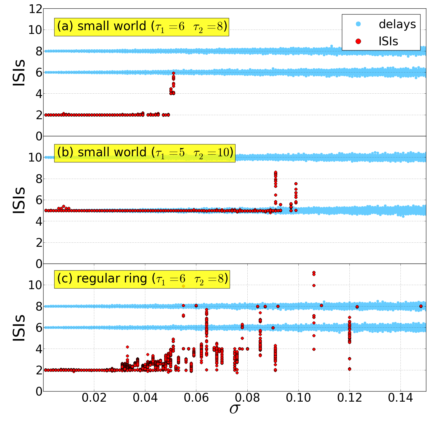
Figure 10: Interspike intervals (ISIs) (red dots) and delay distributions (blue dots) vs $\sigma\equiv\sigma^{(1)}=\sigma^{(2)}$ for different combinations of mean delay times. (a), (b): small-world network ($k=2$, $p=0.51$), (c): regular ring network ($k=2$). Mean delay times are $\tau_{1}=6$ and $\tau_{2}=8$ for (a) and (c), and $\tau_{1}=5$ and $\tau_{2}=10$ for (b). $N=50$. Other parameters as in Fig. 1.

\begin{overpic}[width=433.62pt]{fig11.png} \put(6.6,72.5){(a)} \put(6.6,55.0){(b)} \put(6.6,21.5){(c)} \put(56.0,72.5){(d)} \put(56.0,55.0){(e)} \put(56.0,21.5){(f)} \end{overpic}

Figure 11: Dynamics for a bimodal delay distribution in a regular ring with $k=2$ for different $\sigma$: (a)-(c) $\sigma=0.05$; (d)-(f)$\sigma=0.08$. (a) and (d): time series of $u_{0}$ (dark red) and $v_{0}$ (light blue); (b) and (e): phase portraits of a single spiking node $(u_{0},v_{0})$: trajectory (red solid) and $u$-nullcline (blue dashed); (c) and (e): spiking patterns. Mean delay times $\tau_{1}=6$, $\tau_{2}=8$. Other parameters as in Fig. 1.

6 Conclusion

We have studied the effects of heterogeneous coupling delays in complex networks of excitable elements. As a model we have used the FitzHugh- Nagumo system which is generic for excitability of type II, i.e., close to a Hopf bifurcation. We have investigated two discrete delay times as well as uni- and bimodal continuous distributions. As topologies we have considered regular, small-world, and random networks.

In case of unimodal distributions, we have found three different dynamical scenarios: For narrow distributions the network fires in a highly synchronized mode, because it behaves almost as expected for a network with only one discrete delay time equal to the mean of the distribution. Thus, such networks can be described in good approximation by a discrete delay time which allows for further analysis, for example, using the master stability function. If the width of the distribution is increased, states might arise where the network still fires but with reduced synchronicity. Whether such states, for instance traveling disruption patterns, subnetwork synchronization, or partial amplitude death, exist depends on the topology since they require a certain degree of regularity found in regular rings and to a lesser extent also in small-world networks. In contrast, in random networks, i.e., in the absence of any regularity, such dynamics is hardly found. If the width of the delay distribution becomes too large, global amplitude death is induced.

Global amplitude death has first been observed by Reddy et. al. in delay-coupled Stuart-Landau oscillators RED98 . They showed that an appropriate choice of the delay time changes the stability of the fixed point and yields global amplitude death. In contrast, FitzHugh-Nagumo is an excitable system. Thus, delay in the coupling is needed to generate self-sustained oscillation with a period close to the delay time PAN12 . However, as we show, if the delay distribution becomes too large the delay cannot play this constructive role any longer.

The phenomena of partial amplitude death has been first investigated by Atay in two coupled weakly nonlinear oscillators ATA03a . However, there partial amplitude death was induced by heterogeneities in the nodes, while here we focus on delay heterogeneities.

Masoller et. al. studied Gaussian and exponentially distributed delays in networks of logistic maps MAS11a . They also find synchronous oscillating dynamics for narrow delay distributions and amplitude death for wider distributions. However, the network topology plays a different role; for logistic maps subnetwork synchronization is possible in random networks, while we see this dynamical behavior only in regular and (rarely) in small-world networks.

Furthermore, we investigated two discrete delay time and biomodial distributions. The dynamics in networks with two discrete delay times is characterized by resonance effects, similar to the effects observed in small network motifs SCH08 ; PAN12 , independent of topology. If a resonance condition is fulfilled the network spikes coherently with an interspike interval which is described by a simple linear relation.

Bimodal distributions combine the features of the two cases discussed above: They are characterized by two dominant mean delay times, but with a distribution of the delays around these two peaks with some widths. Hence, we observe dynamical patterns which we already encountered in the two other cases. If the widths around the two mean delays are small, the network behaves as in the case of two discrete delay times and resonance effects play a major role. If the widths of the distributions increases, we see dynamical scenarios already present in the case of unimodal distributions with intermediate width. In particular, in regular networks and small-world networks we see that several subnetworks coexist which spike with different interspike intervals. For large distribution widths, amplitude death is the only dynamical state which we have found.

In summary, networks with narrow delay distributions can be well described by discrete delays, but as the width of the distribution increases, topological features have to be taken into account as they can give rise to more complex dynamics. In networks with broad distributions spiking is not possible any longer and initial excitations die out fast, leading to global amplitude death. This behavior is similar to the case of only two coupled oscillators with distributed delay in the link between them, where the regime of amplitude death increases with the width of the delay kernel ATA03 ; KYR11 ; KYR13 . The robustness of highly synchronous spiking against heterogeneous delays is best for random networks, and worst for large regular networks, and intermediate for small-world networks. In contrast, large regular networks are more robust than random or small-world networks with respect to avoiding global amplitude death, since they can allow stable subnetwork spiking more easily.

Acknowledgments.

This work was supported by the DFG in the framework of the SFB 910.

References

- (1) A.S. Pikovsky, M.G. Rosenblum, J. Kurths, Synchronization, A Universal Concept in Nonlinear Sciences (Cambridge University Press, Cambridge, 2001)
- (2) P. Roelfsema, A. Engel, P. K nig, W. Singer, Nature 385, 157 (1997)
- (3) K. Poeck, W. Hacke, Neurologie, 11th edn. (Springer, Heidelberg, 2001)
- (4) E. Rossoni, Y. Chen, M. Ding, J. Feng, Phys. Rev. E 71, 061904 ( 11) (2005)
- (5) W. Singer, Scholarpedia 2, 1657 (2007)
- (6) R. Vicente, L.L. Gollo, C.R. Mirasso, I. Fischer, P. Gordon, Proc. Natl. Acad. Sci. U.S.A. 105, 17157 (2008)
- (7) C. Masoller, M.C. Torrent, J. García-Ojalvo, Phys. Rev. E 78, 041907 (2008)
- (8) J. Lehnert, T. Dahms, P. Hövel, E. Schöll, Europhys. Lett. 96, 60013 (2011)
- (9) I. Kanter, E. Kopelowitz, R. Vardi, M. Zigzag, W. Kinzel, M. Abeles, D. Cohen, Europhys. Lett. 93, 66001 (2011)
- (10) T. Pérez, G.C. Garcia, V.M. Eguiluz, R. Vicente, G. Pipa, C. Mirasso, PLoS ONE 6, e19900 (2011)
- (11) A. Keane, T. Dahms, J. Lehnert, S.A. Suryanarayana, P. Hövel, E. Schöll, Eur. Phys. J. B 85, 407 (2012)
- (12) L.M. Pecora, T.L. Carroll, Phys. Rev. Lett. 80, 2109 (1998)
- (13) J. Kestler, W. Kinzel, I. Kanter, Phys. Rev. E 76, 035202 ( 4) (2007)
- (14) F. Sorrentino, E. Ott, Phys. Rev. E 76, 056114 ( 10) (2007)
- (15) T. Dahms, J. Lehnert, E. Schöll, Phys. Rev. E 86, 016202 (2012)
- (16) C. Koch, Biophysics of Computation: Information Processing in Single Neurons (Oxford University Press, New York, 1999)
- (17) R. FitzHugh, Biophys. J. 1, 445 (1961)
- (18) J. Nagumo, S. Arimoto, S. Yoshizawa., Proc. IRE 50, 2061 (1962)
- (19) B. Lindner, J. García-Ojalvo, A. Neiman, L. Schimansky-Geier, Phys. Rep. 392, 321 (2004)
- (20) M. Heinrich, T. Dahms, V. Flunkert, S.W. Teitsworth, E. Schöll, New J. Phys. 12, 113030 (2010)
- (21) J.D. Murray, Mathematical Biology, Vol. 19 of Biomathematics Texts, 2nd edn. (Springer, Berlin Heidelberg, 1993)
- (22) E.M. Izhikevich, Int. J. Bifurc. Chaos 10, 1171 (2000)
- (23) D.J. Watts, S.H. Strogatz, Nature 393, 440 (1998)
- (24) R. Monasson, Eur. Phys. J. B 12, 555 (1999)
- (25) M.E.J. Newman, D.J. Watts, Phys. Lett. A 263, 341 (1999)
- (26) A. Rapoport, Bull. Math. Biol. 19, 257 (1957)
- (27) R. Solomonoff, A. Rapoport, Bull. Math. Biol. 13, 107 (1951)
- (28) P. Erdős, A. Rényi, Publ. Math. Debrecen 6, 290 (1959)
- (29) P. Erdős, A. Rényi, Publ. Math. Inst. Hung. Acad. Sci 5, 17 (1960)
- (30) Y. Kuramoto, Chemical Oscillations, Waves and Turbulence (Springer-Verlag, Berlin, 1984)
- (31) M.G. Rosenblum, A.S. Pikovsky, J. Kurths, C. Schäfer, P.A. Tass, Phase synchronization: from theory to data analysis (Elsevier Science, Amsterdam, 2001), Vol. 4 of Handbook of Biological Physics, chap. 9, pp. 279–321, 1st edn.
- (32) E. Schöll, G. Hiller, P. Hövel, M.A. Dahlem, Phil. Trans. R. Soc. A 367, 1079 (2009)
- (33) A. Panchuk, D.P. Rosin, P. Hövel, E. Schöll, Int. J. Bif. Chaos 23, 1330039 (2013)
- (34) M. Zigzag, M. Butkovski, A. Englert, W. Kinzel, I. Kanter, Europhys. Lett. 85, 60005 (2009)
- (35) D.V.R. Reddy, A. Sen, G.L. Johnston, Phys. Rev. Lett. 80, 5109 (1998)
- (36) F.M. Atay, Physica D 183, 1 (2003)
- (37) C. Masoller, F.M. Atay, Eur. Phys. J. D 62, 119 (2011)
- (38) F.M. Atay, Phys. Rev. Lett. 91, 094101 (2003)
- (39) Y.N. Kyrychko, K.B. Blyuss, E. Schöll, Eur. Phys. J. B 84, 307 (2011)
- (40) Y.N. Kyrychko, K.B. Blyuss, E. Schöll, Phil. Trans. R. Soc. A 371, 20120466 (2013)