Visualizing the Effects of a Changing Distance on Data Using Continuous Embeddings

Abstract

Most Machine Learning (ML) methods, from clustering to classification, rely on a distance function to describe relationships between datapoints. For complex datasets it is hard to avoid making some arbitrary choices when defining a distance function. To compare images, one must choose a spatial scale, for signals, a temporal scale. The right scale is hard to pin down and it is preferable when results do not depend too tightly on the exact value one picked. Topological data analysis seeks to address this issue by focusing on the notion of neighbourhood instead of distance. It is shown that in some cases a simpler solution is available. It can be checked how strongly distance relationships depend on a hyperparameter using dimensionality reduction. A variant of dynamical multi-dimensional scaling (MDS) is formulated, which embeds datapoints as curves. The resulting algorithm is based on the Concave-Convex Procedure (CCCP) and provides a simple and efficient way of visualizing changes and invariances in distance patterns as a hyperparameter is varied. A variant to analyze the dependence on multiple hyperparameters is also presented. A cMDS algorithm that is straightforward to implement, use and extend is provided. To illustrate the possibilities of cMDS, cMDS is applied to several real-world data sets.

1 Introduction

The notion of distance is at the core of data analysis, pattern recognition and machine learning: most methods need to know how similar two datapoints are. The choice of distance metric is often a hidden assumption in algorithms. For complex data, distance or similarity are not uniquely defined. On the contrary, they can be arbitrary to some extent [Carlsson2009]. It is, for example, often possible to describe signals on different temporal or spatial scales, and distance functions will give a certain scale more weight than another. Each datapoint might describe several features, and there is often no unique, optimal way to weigh the features when computing a distance measure: are two individuals more alike if they have similar eye colour or hair colour, or do we think the shape of the nose matters most?

There are ways around that problem. One is to select the distance function that is best adapted to the task at hand, for example the one that gives the best performance in classification (this is effectively what is done in kernel hyperparameter selection [Scholkopf2002]). Another is to give up on distance and rely instead on the weaker notion of neighbourhood [Lum2013].

We argue here that a third option is available. One may study how the shape of the data evolves under a change in the distance metric by representing the data in lower dimension. We suppose that a family of distance functions $d_{\alpha}(x,y)$ is defined by varying a hyperparameter $\alpha\in[0,1]$, where $\alpha$ can represent, for example, different scales or the mixing proportion of features. Please note that $\alpha$ does not have to be defined on this interval, but it seems natural to start with a setting that is familiar from, e.g., convex combinations. Suppose that for a given level of $\alpha$ the relative distances between datapoints are well described by representing the datapoints as points on the line. As we vary $\alpha$ the points will move, so that each point now describes a curve. Many scenarios are possible, and we sketch them in Fig. 1. We may have full or partial invariance: patterns in the data that hold regardless of the value of the hyperparameter (Fig. 1A). On the other hand, the structure in the data may appear only for certain values of $\alpha$ (intermediate values in Fig. 1B and rather small values in C), indicating that these values are more useful than others for characterizing the data. Analyzing the evolution of structures in the data might reveal interesting dependencies, for example, declustering (Fig. 1C) or loss of information (Fig. 1D).

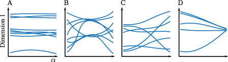
Figure 1: Sketches of different effects on the data structure that emerge when varying a hyperparameter in a distance function. The $x$-axis shows the hyperparameter $\alpha$, the $y$-axis is the embedding dimension. A) Invariance: patterns hold independent of the hyperparameter. B/C) Structure emerges only for certain values of the hyperparameter. C) Declustering: clusters are lost with increasing hyperparameter. D) Information loss: Structure collapses with increasing hyperparameter.

To visualize the effects of varying the distance function we suggest to embed data into a space of smooth curves, forming what we call continuous embeddings: in continuous embeddings each datapoint is embedded as a smooth curve in $\mathbb{R}^{d}$. We will show that this approach is quite general.

Our implementation of continuous embeddings is based on multi-dimensional scaling (MDS), one of the most widely-used tools for dimensionality reduction [Buja2002, Buja2008]. MDS builds on the pairwise relation between single data points and has an intuitive way of characterizing the structure in high-dimensional data. MDS supposes that one has distance information available, that is, we can characterize the data by a distance matrix. MDS seeks to find a set of points in a low dimensional Euclidean space, such that the Euclidean distances between points approximate the original distances. An exception is spherical MDS, where the embedding is constrained to a spherical manifold. MDS goes back to the 1950s, when it was first introduced as classical scaling [Torgerson1952]. In classical scaling, the distance matrix is transformed to a matrix of inner products from which an embedding can be computed using eigendecompositions [Torgerson1952, Torgerson1958, Gower1966]. Classical scaling finds a perfect embedding when the data can indeed be embedded exactly, but in all realistic cases distance matrices are not exactly Euclidean and distance scaling is more appropriate. Kruskal1964 introduced distance scaling by defining a cost function, Stress, that directly measures the error between original and embedding distances. This cost function is then optimized over the space of embedding matrices which can be done using gradient descent. Since the early work on MDS many other variants and optimization solutions have been discussed. So called non-metric variants of MDS seek to only recover the ranks of distances [Shepard1962]. Ramsay1977, Ramsay1978 introduces a statistical model for MDS, allowing for a maximum likelihood estimate. This approach is implemented in Multiscale [Ramsay1978b]. Other MDS variants based on Stress include Sammon’s mapping [Sammon1969], elastic stress [McGee1966], multidimensional unfolding [Borg2005] and local MDS [Chen2009]. Isomap [Tenenbaum2000] is also related to MDS. Here, distances are computed as geodesic distances on a manifold, which are then embedded with classical scaling. In terms of optimization one of the most popular approaches is SMACOF, a majorization method for MDS [Guttman1968, DeLeeuw1977, DeLeeuw1977b, DeLeeuw1988].

Here, we introduce a continuous version of MDS (cMDS) by adding a smoothing penalty to the MDS cost function. Similar ideas have been used in the visualization of dynamic networks. A network is commonly represented as a graph. A 2D embedding of a static graph is often constructed using MDS or similar methods [Kamada1989, Gansner2005]. In the dynamical context, where a graph is measured over time, it is important to preserve the so-called “mental map” when jumping from one timepoint to the next [Misue1995]. Early work on such controlled stability was done by Boehringer1990, North1996. Brandes1997 developed a more rigorous formulation of controlled stability based on regularization in a Bayesian framework. There have been three different approaches to the problem of preservation of the mental map: aggregation, anchoring and linking. In aggregation methods, the graph is aggregated into an average graph which is then visualized with a static layout algorithm [Brandes2003, Moody2005]. Anchoring methods use auxiliary edges which connect nodes to stationary reference positions [Brandes1997, Diehl2002, Frishman2008]. In linking, edges are created that connect instances of a single vertex over time. The resulting graph is then visualized using standard methods [Erten2004, Erten2004b, Dwyer2006]. Linking has been formulated in more rigorous ways in terms of regularized cost functions [Baur2008, Brandes2012a]. Xu2013 introduce an additional grouping penalty. Brandes2012a provide a good overview on dynamic graph layout. Another approach to dynamic embeddings is an extension of the Hoff latent space model [Sarkar2005]. In functional MDS [Masahiro2003], individual solutions to the MDS problems are rotated in a secondary step to minimize the length of the curves. This does not allow for control of smoothness versus stress, which is true for most methods described above.

All these approaches and contributions in the field visualize temporal developments. We show here that continuous embeddings can be applied to a great variety of data, going far beyond the visualization of temporal dynamics in graphs. In particular, the continuous variable can be used to visualize artificial dynamics. This makes the method very general and is especially useful in the analysis of families of distance functions and their effects on data structure. Continuous embeddings are thus a tool for making an informed choice of the distance metric for use in further analyses.

We show how continuous embeddings can be efficiently computed using the Concave-Convex Procedure (CCCP) for optimization [Yuille2003]. The resulting algorithm is a simple iterative procedure, in which the inner loops are nothing more than least squares regression with smoothing splines. We prove that the algorithm always leads to a stationary point. This goes further than other proofs [Sriperumbudur2009, Yen2012] because the cost function is nondifferentiable at certain points and doesn’t share the directional derivative with the upper bound at those points. We provide an R package for cMDS which is available on github: github.com/ginagruenhage/cmdsr. We illustrate the results of cMDS with several examples. We compare cMDS to a method based on $k$-means to exemplify that cMDS provides a more informative way of understanding the data structure. We show that cMDS leads to novel forms of data visualization and enhances the analysis of various meta-effects in data, such as hierarchy levels in hierarchical clustering, weighting of different distance measures and consensus requirements across subjects. Furthermore, we point out that quantitative analyses on cMDS results are possible and useful. We show that cMDS is especially well-suited to dynamic and interactive contexts [Cook2007]. We provide several examples of interactive, web-based visualizations based on cMDS.

2 Methods

In order to present the cMDS algorithm, we introduce some notations and definitions. We describe the objective of the algorithm and present the cost function that we need to optimize. Optimization can be done in a coordinate-wise manner and we present the optimization of single coordinates via the Concave-Convex Procedure and pseudocode of the full algorithm in Section 2.2. In the subsequent section, we prove that the optimization of single coordinates is first-order optimal, i.e. it leads to stationary points of the original cost. We also show that this directly entails first order optimality of the full cost.

We start by setting the notations. The original data or objects are denoted by $\mathbf{s}_{1}(\alpha)\,\ldots\,\mathbf{s}_{N}(\alpha)$, where $N$ is the number of objects in the data. The objects are defined in an arbitrary metric space, e.g. $\mathbb{R}^{D}$. The parameter $\alpha$ measures a continuous dimension. We will see that objects, such as images or networks, can be endowed with a continuous dimension, for example by examining them at different scales, so that scale plays the role of the continuous parameter. At this point we would like to note that we discretize all equations from the beginning, because ultimately, in the implementation, the hyperparameter has to be discretized. It would certainly be possible to develop all the mathematics in a continuous matter. We prefer to present the mathematics in such a way that the equations in the paper can be used as a direct reference for implementation. However, important equations, such as the cost function and the penalty are given in their continuous form as well, to improve the understanding of the problem definition. Thus, $\alpha$ is represented on a grid $\alpha_{1}\,\ldots\,\alpha_{T}$. We use $T$ to denote the maximum value of $\alpha$ since time is the most natural framework to think about the hyperparameter. With $f(\cdot)$ we refer to function values at all grid points while $f(k)$ refers to a function value at a specific value of $\alpha$. The objects are endowed with a distance function $d\left(x,y\right)$. The appropriate distance function depends on the data-space and on the nature of the problem. Given a distance measure, we can define a distance array, $\mathbf{D}^{(\cdot)}\in\mathbb{R}^{T\times N\times N}$, where the entry $d_{ij}^{k}$ holds the distance between objects $\mathbf{s}_{i}$ and $\mathbf{s}_{j}$ at $\alpha_{k}$. We assume that the distances between datapoints give a good summary of the patterns in the data. The goal of cMDS will be to extract these patterns.

2.1 Objective

The objective of cMDS is to retrieve curves or manifolds in $\mathbb{R}^{d}$, $d<<D$ which we denote as $\mathbf{x}^{(\cdot)}_{1}\,\ldots\,\mathbf{x}^{(\cdot)}_{N}\in\mathbb{R}^{T\times d}$, such that the evolution of distances between the curves represents the evolution of distances between the datapoints. When we talk about curves, we mean the technical differential geometry sense of the word, namely, a curve is a 1-dimensional manifold in $\mathbb{R}^{d}$. The curves are represented as a configuration array $\mathbf{X}^{(\cdot)}\in\mathbb{R}^{T\times d\times N}$ and for a given time-point $\alpha_{k}$ $\mathbf{X}^{k}$ is a $d\times N$ matrix in which each column represents the coordinates of a curve at time $\alpha_{k}$. In $\mathbb{R}^{d}$ we measure the distance between two curves at $\alpha_{k}$ with the Euclidean distance. Thus, for each configuration, we have a distance array $\mathbf{\tilde{D}}^{(\cdot)}\in\mathbb{R}^{T\times N\times N}$ such that $\tilde{d}_{ij}^{k}=\lVert\mathbf{x}^{k}_{i}-\mathbf{x}^{k}_{j}\rVert_{2}$. To denote that $\mathbf{\tilde{D}}^{(\cdot)}$ is computed from $\mathbf{X}^{(\cdot)}$, we occasionally write $\mathbf{\tilde{D}}^{(\cdot)}\left(\mathbf{X}^{(\cdot)}\right)$. These are the approximate distances given by our embedding, and the objective is to make the approximate distances as close as possible to the real distances. A natural expression of that objective is the following cost function, which quantifies the distortion of the embedding:

$$\mathcal{L}\left(\mathbf{X}^{(\cdot)},\mathbf{D}^{(\cdot)}\right)=\int_{0}^{1}\left(\lVert\mathbf{\tilde{D}}^{\alpha}(\mathbf{X}^{\alpha})-\mathbf{D}^{\alpha}\rVert_{F}\right)^{2}\mbox{d}\alpha,$$ (1)

where $\lVert\cdot\rVert_{F}$ denotes the Frobenius norm. This is the MDS cost function for continous data. Its discretized form is:

$$\mathcal{L}\left(\mathbf{X}^{(\cdot)},\mathbf{D}^{(\cdot)}\right)=\sum_{k=1}^{T}\left(\lVert\mathbf{\tilde{D}}^{k}(\mathbf{X}^{k})-\mathbf{D}^{k}\rVert_{F}\right)^{2}.$$ (2)

In practice and for real datasets, MDS is a highly non-convex optimization problem with multiple local minima. Additionally, since distances are invariant to rotations, translations and symmetries, so are the MDS embeddings. Minimizing (2) is equivalent to solving MDS problems for different values of the hyperparameter individually. The individual problems are known as Kruskal-Shephard scaling [Kruskal1964]. This would result in solutions that are independent for different $\alpha_{k}$ and thus might lie in quite different local minima. However, one would expect that slight changes in the hyperparameter lead to only slight changes in the embedding. To solve this problem, we will require that each curve is continuous and smooth, which can be achieved by adding a suitable penalty function $\Omega(\mathbf{X}^{(\cdot)})$ to the cost. The effect of the smoothing penalty can be interpreted as the goal of tracing one particular local minimum across different values of the hyperparameter. This results in the cost function

$$\mathcal{C}\left(\mathbf{X}^{(\cdot)},\mathbf{D}^{(\cdot)}\right)={\mathcal{L}\left(\mathbf{X}^{(\cdot)},\mathbf{D}^{(\cdot)}\right)+\lambda\,\Omega\left(\mathbf{X}^{(\cdot)}\right)}.$$ (3)

Classical spline penalties [Ramsay1997] are particularly convenient. We introduce the penalty in its continous form:

$$\Omega\left(\mathbf{X}(\alpha)\right)=\int_{0}^{1}\left\|\frac{\partial^{2}\mathbf{x}(\alpha)}{\partial\alpha^{2}}\right\|\mbox{d}\alpha.$$ (4)

In practice, we work with discrete one-dimensional manifolds in $\mathbb{R}^{d}$ for which the penalty reads

rCl Ω(X^(⋅)) & = ∑_d diag( ∑_i (x^(⋅)_i)^T  (D^(2))^T D^(2)  x^(⋅)_i)
= ∑_d diag(∑_i (x^(⋅)_i)^T  M   x^(⋅)_i ), where $\mathcal{D}^{(2)}$ denotes the discrete second order differential operator. The parameter $\lambda$ controls how strongly the roughness of the curves is penalized. For $\lambda=0$, we recover the classical cost function of MDS, with the extension that we have $T$ separate MDS problems, one for each value of $\alpha$. For $\lambda\rightarrow\infty$ the resulting curves are straight lines, independent of the original data. The value of $\lambda$ is easy to set by visual inspection. It should simply be large enough to result in fairly smooth curves, while keeping the distortion reasonably small. A reasonable strategy for setting $\lambda$ automatically is then to maximize $\lambda$, under a constraint on the quality of the embedding. This quality can be measured in various ways [Kaski2011, Mokbel2013]. The effect of the smoothing parameter $\lambda$ is shown in a supplemenatry material file.

2.2 Optimization via the Concave-Convex Procedure (CCCP)

The cMDS algorithm optimizes the cost in a curve-by-curve manner. This is possible since the cost is a sum over costs per curve. Thus, we have an outer loop over curves and an inner loop that performs conditional optimization on $\mathbf{x}^{(\cdot)}_{i}$. That is, we assume that all curves $\mathbf{x}^{(\cdot)}_{j},j\neq i$ are fixed. The inner loop is a Maximization Minimization procedure. Specifically, we use the Concave-Convex Procedure (CCCP) [Yuille2003]. This way, each minimization step is a simple spline regression. In effect, the algorithm only needs to compute spline regressions with surrogate data.

We now outline the usage of CCCP for the optimization of a single curve. We expand the first term of the cost function to identify the convex and concave parts. We denote the cost of a single curve as $f(\cdot)$:

rCl f(x^(⋅)_i) & = ∑_kj ( ∥ x^k_i - x^k_j∥_2 - d_ij^k )^2+ λ(x^(⋅)_i)^T  M  x^(⋅)_i
= ∑_kj(x^k_i - x^k_j)^T(x^k_i-x^k_j)
- ∑_kj 2 d_ij^k ∥x^k_i - x^k_j∥ + ∑_kj (d_ij^k)^2
+  λ  (x^(⋅)_i)^T  M  x^(⋅)_i
= f_vex(x^(⋅)_i) + f_cave(x^(⋅)_i) + const, where

$$f_{vex}\bigl{(}\mathbf{x}^{(\cdot)}_{i}\bigr{)}=\sum_{kj}(\mathbf{x}^{k}_{i}-\mathbf{x}^{k}_{j})^{T}(\mathbf{x}^{k}_{i}-\mathbf{x}^{k}_{j})+\lambda\,(\mathbf{x}^{(\cdot)}_{i})^{T}\,\mathbf{M}\,\mathbf{x}^{(\cdot)}_{i}$$ (5)

and

$$f_{cave}\bigl{(}\mathbf{x}^{(\cdot)}_{i}\bigr{)}=-\sum_{kj}2\,d_{ij}^{k}\left\|\mathbf{x}^{k}_{i}-\mathbf{x}^{k}_{j}\right\|.$$ (6)

In the optimization, we can omit the constant term that doesn’t depend on $\mathbf{x}^{(\cdot)}_{i}$. The iterative CCCP algorithm $(\mathbf{x}^{(\cdot)}_{i})^{t-1}\mapsto(\mathbf{x}^{(\cdot)}_{i})^{t}$ is given by

$$(\mathbf{x}^{(\cdot)}_{i})^{t}=\operatorname*{arg\,min}_{\mathbf{x}^{(\cdot)}_{i}}\;\;u\bigl{(}\mathbf{x}^{(\cdot)}_{i},(\mathbf{x}^{(\cdot)}_{i})^{t-1}\bigr{)},$$ (7)

where the convex upper bound is computed by taking the first-order Taylor expansion of the concave part of $f$. The concave part is, however, non-differentiable at $\mathbf{x}^{k}_{i}=\mathbf{x}^{k}_{j}$. We thus work with a modified subdifferential.

rCl 3l→∇^SD f_cave((x^k_i)^t-1)
 & = 2 ∑_k∑_i d_ij^k {(xki)t-1- xkj∥(xki)t-1- xkj∥if $(\mathbf{x}^{k}_{i})^{t-1}\neq\mathbf{x}^{k}_{j}${u : ∥u ∥= 1 }if $(\mathbf{x}^{k}_{i})^{t-1}=\mathbf{x}^{k}_{j}$. In the latter case, $\mathbf{u}$ is chosen randomly. The usual definition of the subdifferential [Rockafellar1970] would yield a less strong condition on $\mathbf{u}$, namely $\left\|\mathbf{u}\right\|\leq 1$. We choose the stronger variant to achieve maximum descent in each optimization step. We introduce surrogate points $\hat{\mathbf{x}}^{(\cdot)}_{j}$.

$$\hat{\mathbf{x}}^{k}_{j}=\mathbf{x}^{k}_{j}+d_{ij}^{k}\begin{cases}\frac{(\mathbf{x}^{k}_{i})^{t-1}-\mathbf{x}^{k}_{j}}{\left\|(\mathbf{x}^{k}_{i})^{t-1}-\mathbf{x}^{k}_{j}\right\|}&\text{if $(\mathbf{x}^{k}_{i})^{t-1}\neq\mathbf{x}^{k}_{j}$}\\ \left\{\mathbf{u}:\lVert\mathbf{u}\rVert=1\right\}&\text{if $(\mathbf{x}^{k}_{i})^{t-1}=\mathbf{x}^{k}_{j}$}\end{cases},$$ (8)

where, again, $\mathbf{u}$ is chosen randomly.

The resulting upper bound for the original cost is

rCl u( (x^(⋅)_i)^t, (x^(⋅)_i)^t-1) & = ∑_kj ((x^k_i)^t - x^k_j)^T((x^k_i)^t-x^k_j)
-  2 ∑_kj d