The complex singularity of a Stokes wave The complex singularity of a Stokes wave S. A. Dyachenko, P. M. Lushnikov, and A. O. Korotkevich Dyachenko, Lushnikov, Korotkevich 6 November 2013*

The complex singularity of a Stokes wave

Abstract

Two-dimensional potential flow of the ideal incompressible fluid with free surface and infinite depth can be described by a conformal map of the fluid domain into the complex lower half-plane. Stokes wave is the fully nonlinear gravity wave propagating with the constant velocity. The increase of the scaled wave height $H/\lambda$ from the linear limit $H/\lambda=0$ to the critical value $H_{max}/\lambda$ marks the transition from the limit of almost linear wave to a strongly nonlinear limiting Stokes wave. Here $H$ is the wave height and $\lambda$ is the wavelength. We simulated fully nonlinear Euler equations, reformulated in terms of conformal variables, to find Stokes waves for different wave heights. Analyzing spectra of these solutions we found in conformal variables, at each Stokes wave height, the distance $v_{c}$ from the lowest singularity in the upper half-plane to the real line which corresponds to the fluid free surface. We also identified that this singularity is the square-root branch point. The limiting Stokes wave emerges as the singularity reaches the fluid surface. From the analysis of data for $v_{c}\to 0$ we suggest a new power law scaling $v_{c}\propto(H_{max}-H)^{3/2}$ as well as new estimate $H_{max}/\lambda\simeq 0.1410633$.

02.60Cb, 47.10.-g, 47.35.Bb, 92.10.Hm

Theory of spatially periodic progressive (propagating with constant velocity without change of the amplitude) waves in two-dimensional (2D) potential flow of an ideal incompressible fluid with free surface in gravitational field was founded in pioneering works by Stokes [1, 2] and developed further by Michell [3], Nekrasov [4, 5], and many others (see e.g. a book by Sretenskii [6] for review of older works as well as Refs. [7, 8, 9, 10, 11, 12, 13, 14] and Refs. there in for more recent progress). There are two major approaches to analyze the Stokes wave, both originally developed by Stokes. The first approach is the perturbation expansion in amplitude of Stokes wave called by the Stokes expansion. That approach is very effective for small amplitudes but converges very slowly (or does not converge at all, depending on the formulation) as the wave approaches to the maximum height $H_{max}$ (also called by the wave of the greatest height or the limiting Stokes wave) which is defined at the distance from the crest to the trough of Stokes wave over a spatial period $\lambda$. The second approach is to consider a limiting Stokes wave, which is the progressive wave with the highest nonlinearity. Stokes found that the limiting Stokes wave has the sharp angle of $2\pi/3$ radians on the crest [15], i.e. the surface is non-smooth (has a jump of slope) at that spatial point. That corner singularity explains a slow convergence of Stokes expansion as $H\to H_{max}.$

It was Stokes [15] who proposed to use conformal mapping in order to address finite amplitude progressive wave. In this letter we consider the particular case of infinite depth fluid although more general case of fluid of arbitrary depth can be studied in a similar way. Assume that the free surface is located at $y=\eta(x,t)$, where $x$ is the horizontal coordinate, $y$ is the vertical coordinate, $t$ is the time and $\eta(x,t)$ is the surface elevation with respect to the mean level of fluid, i.e. $\int^{\infty}_{-\infty}\eta(x,t)dx=0$. We consider the conformal map of the domain $-\infty<y<\eta(x,t),\ -\infty<x<\infty$ of the complex plane $z\equiv x+iy$ filled by the infinite depth fluid into a lower complex half-plane (from now on denoted by $\mathbb{C^{-}}$) of a variable $w\equiv u+iv$ (see Fig. 1). The free surface is mapped into the real line $v=0$ with $z(w)$ being the analytic function in the lower half-plane of $w$ as well as the complex fluid potential $\Pi(w)$ is also analytic in $\mathbb{C^{-}}$.

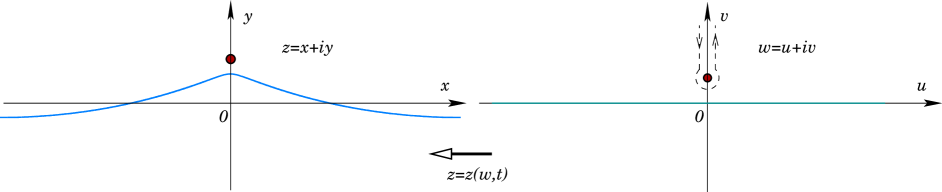
Figure 1: Fig. 1. Schematic of a conformal map between the domain below the solid line (left panel) in $z=x+iy$ plane and the lower half-plane in $w=u+iv$ (right panel). Fluid occupies the domain below the solid line in physical plane $z=x+iy.$ The solid line of left panel (corresponds to a free surface of the fluid) is mapped into the real line (another solid line) in right panel. One spatial period of Stokes wave is shown by solid lines in both panels in the reference frame moving with the velocity $c$. The dark circles mark the positions of the singularity closest to the fluid surface in both panels. The dashed line in right panel shows the integration contour as it is moved from the real line upward, see text for more details.

Both $z(w)$ and $\Pi(w)$ have singularities in upper half-plane (here and further denoted by $\mathbb{C}^{+}$). The knowledge of singularities in $\mathbb{C}^{+}$ would result in the efficient description of the solution in the physical variables. Examples of such type of solutions in hydrodynamic-type systems are the dynamics of free surface of ideal fluid with infinite depth [16] and finite depth [17], dynamics of interface between two ideal fluids [18], ideal fluid pushed through viscous fluid in a narrow gap between two parallel plates (Hele-Shaw flow) [19] and the dynamics of the interface between ideal fluid and light viscous fluid [20]. In all these systems the dynamics is determined by poles/branch cuts in the complex plane.

In this Letter we determine that for Stokes wave the lowest singularities in $\mathbb{C}^{+}$ of both $z(w)$ and $\Pi(w)$ are the square-root branch points located periodically at $w=n\lambda+iv_{c}-ct,\ n=0,\pm 1,\pm 2,...$ (we choose that the crests of Stokes wave to be located at $w=n\lambda-ct$) and we determine $v_{c}$ numerically as a function of $H/\lambda$. Here $c$ is the velocity of propagation of Stokes wave which depends on $H$. We found that as $H\to H_{max}$, the branch point approaches real axis with the scaling law

$$v_{c}\propto(H_{max}-H)^{\delta},$$ (1)

where $\delta=1.48\pm 0.03$. At $H=H_{max}$ the branch point reaches the real axis producing the corner singularity at the free surface of limiting Stokes wave. We believe that this new scaling law provides the efficient way for the description of near-limiting Stokes waves. Adiabatically slow approach of Stokes wave to its limiting form during wave dynamics is one of the possible routes to wave breaking and whitecapping, which are responsible for significant part of energy dissipation for gravity waves [21, 22]. Formation of a close to limiting Stokes wave is also considered to be a probable final stage of evolution of a freak (or rogue) waves in the ocean resulting in formation of approximate limiting Stokes wave for a limited period of time with following wave breaking and disintegration of the wave or whitecapping and attenuation of the freak wave into wave of regular amplitude [23, 24].

Basic equations. In physical coordinates $(x,y)$ a velocity ${\bf v}$ of $2D$ potential flow of inviscid incompressible fluid is determined by a velocity potential $\Phi$ as ${\bf v}=\nabla\Phi$. The incompressibility condition $\nabla\cdot{\bf v}=0$ results in the Laplace equation

$$\nabla^{2}\Phi=0$$ (2)

inside fluid $-\infty<y<\eta(x,t)$. To obtain the closed set of equations we add the decaying boundary condition at large depth $\Phi(x,y,t)|_{y\to-\infty}=0$, the kinematic boundary condition

$$\dfrac{\partial\eta}{\partial t}=\left(-\dfrac{\partial\eta}{\partial x}\dfrac{\partial\Phi}{\partial x}+\left.\dfrac{\partial\Phi}{\partial y}\right)\right|_{y=\eta(x,t)}$$ (3)

and the dynamic boundary condition

$$\left.\left(\dfrac{\partial\Phi}{\partial t}+\dfrac{1}{2}\left(\nabla\Phi\right)^{2}\right)\right|_{y=\eta(x,t)}+g\eta=0$$ (4)

at the free surface $y=\eta(x,t).$ We define the boundary value of the velocity potential as $\left.\Phi(x,y,t)\right|_{y=\eta(x,t)}\equiv\psi(x,t)$.

The system (2)-(4) was recast into the conformal variables first in Ref. [25] and later independently in Ref. [26] taking the following form [26]:

$$y_{t}x_{u}-x_{t}y_{u}+\hat{H}\psi_{u}=0$$ (5)

for the kinematic boundary condition and

$$\psi_{t}y_{u}-\psi_{u}y_{t}+gyy_{u}=-\hat{H}\left(\psi_{t}x_{u}-\psi_{u}x_{t}+gyx_{u}\right)$$ (6)

for the dynamic boundary condition. Here $\hat{H}f(u)=\frac{1}{\pi}P.V.\int^{+\infty}_{-\infty}\frac{f(u^{\prime})}{u^{\prime}-u}du^{\prime}$ is the Hilbert transform with $P.V.$ meaning a Cauchy principal value of integral. Equations (5) and (6) are equivalent to (2)-(4) because $z(w)$ is assumed to be analytic in $\mathbb{C}^{-}$. Both (5) and (6) are defined on the real line $w=u$. Note that a Fourier transform of $\hat{H}$ results in the multiplication operator $(\hat{H}f)_{k}=i\,\text{sign}{\,(k)}\,f_{k}.$ The complex potential $\Pi$ is recovered from the analytical continuation of $(1+i\hat{H})\psi$ into $\mathbb{C}^{-}.$ Also, the analyticity of $z$ in $\mathbb{C}^{-}$ implies that

$$y=\hat{H}\tilde{x}\quad\text{and}\quad\tilde{x}=-\hat{H}y,$$ (7)

where $\tilde{x}(u,t)\equiv x(u,t)-u$ and $\tilde{z}(u,t)\equiv z(u,t)-u.$ We fix the location of fluid surface in $y$ by the condition that the mean elevation $\langle y(1+\tilde{x}_{u})\rangle=0$, where $\langle\ldots\rangle$ stands for the average in $u$.

Progressive waves. Stokes wave corresponds to a solution of system (5) and (6) in the travelling wave form

$$\psi(u,t)=\psi(u-ct),\ \tilde{z}(u,t)=\tilde{z}(u-ct),$$ (8)

where both $\psi$ and $\tilde{z}$ are the periodic functions of $u-ct$. We transform into the moving frame of reference, $u-ct\to u$, and assume that the crest of the Stokes wave is located at $u=0$ as in Fig. 1 and $L$ is the period in $u$ variable for both $\psi$ and $\tilde{z}$ in (8). The Stokes solution requires $y(u)$ to be the even function while $\tilde{x}(u)$ needs to be the odd function. Taking into account the periodicity of $\tilde{x}(u)$ in (8) it implies that $\tilde{x}(\pm L/2)=0$. Then the spatial period of the Stokes solution is the same, $L=\lambda$, both in $x$ variable (i.e. for $\eta(x-ct)$) and $u$ variable (i.e. for (8)).

It follows from (5) and (8) that $\psi=-c\hat{H}y$ and then excluding $\psi$ from (6) we obtain that

$$-c^{2}y_{u}+gyy_{u}+g\hat{H}[y(1+\tilde{x}_{u})]=0$$ (9)

We now apply $\hat{H}$ to (9), use (7) to obtain a closed expression for $y$, and introduce the operator $\hat{k}\equiv-\partial_{u}\hat{H}=\sqrt{-\nabla^{2}}$ which results in the following expression

$$\begin{split}&\hat{L}_{0}y\equiv\left(\dfrac{c^{2}}{c_{0}^{2}}\hat{k}-1\right)y-\left(\frac{\hat{k}y^{2}}{2}+y\hat{k}y\right)=0,\\ \end{split}$$ (10)

where $c_{0}=\sqrt{g/k}$ is the phase speed of linear gravity wave with $k=2\pi/\lambda$ and we made all quantities dimensionless by the following scaling transform $u\to u\lambda/2\pi,\ x\to x\lambda/2\pi,\ y\to y\lambda/2\pi$. In these scaled units the period of $\psi$ and $\tilde{z}$ is $2\pi.$

We solve (10) numerically to find $y(u)$ by two different methods each of them beneficial for different range of parameters. First method is inspired by a Petviashvili method [27] which was originally proposed to find solitons in nonlinear Schrodinger (NLS) equation as well as it was adapted for nonlocal NLS-type equations, see e.g. [28]. Here we use a generalized Petviashvili method (GPM)  [29] designed to solve the general equation $\hat{L}_{0}y\equiv-\hat{M}y+\hat{N}y=0$ for the unknown function $y(u)$, where $\hat{L}_{0}$ is the general operator which includes a linear part $-\hat{M}$ and a nonlinear part $\hat{N}$. For our particular form of $\hat{L}_{0}$ in (10) we have that $-\hat{M}=\left(\dfrac{c^{2}}{c_{0}^{2}}\hat{k}-1\right)$. $\hat{M}$ is invertible on the space of $2\pi$-periodic functions because Stokes wave requires $1<c^{2}/c_{0}^{2}<1.1$ [11]. The convergence of GPM [29, 30] is determined by the smallest negative eigenvalue of the operator $\hat{M}^{-1}\hat{L}$. Here $\hat{L}$ is the linearization operator of $\hat{L}_{0}$ about the solution $y$ of (10): $\hat{L}\delta y=-\hat{M}\delta y-\left(\hat{k}(y\delta y)+y\hat{k}\delta y+\delta y\hat{k}y\right)$. It is assumed that $\hat{M}^{-1}\hat{L}$ has only a single positive eigenvalue $1$ determined by $\hat{L}y=\hat{M}y$. GPM iterations are given by [29]

$$y_{n+1}-y_{n}=\left(\hat{M}^{-1}L_{0}y_{n}-\gamma\dfrac{\langle y_{n},\hat{L}_{0}y_{n}\rangle}{\langle y_{n},\hat{M}y_{n}\rangle}y_{n}\right)\Delta\tau,$$ (11)

where $\Delta\tau>0$ is the parameter that controls a convergence speed of iterations and $\gamma=1+\frac{1}{\Delta\tau}$ is chosen to project iterations into the subspace orthogonal to $y$ (the only eigenfunction $y$ with the positive eigenvalue). In practice this method allowed to find high precision solutions up to $H/\lambda\lesssim 0.1388$ as GPM requires significant decrease of $\Delta\tau$ with the growth of $H/\lambda$ to have convergence. For larger $H/\lambda$ we used the second method which is the Newton Conjugate Gradient (Newton-CG)  method[31, 32]. The idea behind the Newton-CG method is simple and aesthetic: firstly, linearize (10) about the current approximation $y_{n}$: $\hat{L}_{0}y_{n}+\hat{L}_{1}\delta y=0,$ where $\hat{L}_{1}=-\hat{M}\delta y-\left(\hat{k}(y_{n}\delta y)+y_{n}\hat{k}\delta y+\delta y\hat{k}y_{n}\right)$ - linearization of $\hat{L}_{0}$ on the current approximation $y_{n}$. Secondly, solve the resulting linear system for $\delta y$ with one of your favourite numerical methods, in our case it was either Conjugate Gradient (CG) method or Conjugate Residual (CR) method [33] to obtain next approximation $y_{n+1}=y_{n}+\delta y$. It should be noted that monotonic convergence of CG or CR methods are proven only for positive definite (for CR – semidefinite) operators, while in our case $\hat{L}_{1}$ is indefinite. Nevertheless, both methods were converging to the solutions, and convergence was much faster than using GPM.

Newton-CG/CR methods can be written in either Fourier space, or in physical space. We considered both cases, however Newton-CG/CR methods in Fourier space require four fast Fourier transforms per CG/CR step, while in physical space it requires at least six. For both cases CG and CR we used preconditioner $\hat{M}$.

We found that the region of convergence of the Newton-CG/CR methods to nontrivial physical solution (10) is quite narrow and requires an initial guess $y_{0}$ to be very close to the exact solution $y$. In practice we first run GPM and then choose $y_{0}$ for Newton-CG/CR methods as the last available iterate of GPM.

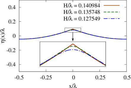
Figure 2: Fig. 2. Stokes wave for $c/c_{0}=1.082500$ (blue line), $c/c_{0}=1.091500$ (green line) and $c/c_{0}=1.0922795$ (dark orange line). Corresponding values of $H/\lambda$ are given in the legend. Inset shows zoom-in into small values of $x/\lambda$ near a wave crest.

Finding singularity from Fourier spectrum. Assume that the singularity of $\tilde{z}$ closest to real axis in $w$ complex plane is the branch point

$$\tilde{z}\simeq c_{1}(w-iv_{c})^{\beta}$$ (12)

for $w\to iv_{c}$, where $c_{1}$ is the complex constant, $v_{c}>0$ and $\beta$ are real constants. By the periodicity in $u$, similar branch points are located at $w=iv_{c}+2\pi n,\,n=\pm 1,\pm 2,\ldots$ We expand $\tilde{z}(u)$ in Fourier series $\tilde{z}(u)=\sum\limits_{k=0}^{-\infty}\hat{\tilde{z}}_{k}\exp[iku]$, where

$$\hat{\tilde{z}}_{k}=\frac{1}{2\pi}\int\limits_{-\pi}^{\pi}\tilde{z}(u)e^{-iku}du$$ (13)

is the Fourier coefficient and the sum is taken over nonpositive integer values of $k$ which ensures both $2\pi$-periodicity of $\tilde{z}(u)$ and analyticity of $\tilde{z}(w)$ in $\mathbb{C}^{-}$. We evaluate (13) in the limit $k\to-\infty$ by moving the integration contour from $-\pi<u<\pi$ into $\mathbb{C}^{+}$ until it hits the lowest branch point (12) so it goes around branch point and continues straight upwards about both side of the corresponding branch cut as shown by the dashed line in right panel of Fig. 1. Here we assume that branch cut is a straight line connecting $w=iv_{c}$ and $+i\infty$. Then the asymptotic of $|\hat{\tilde{z}}_{k}|$ is given by

$$|\hat{\tilde{z}}_{k}|\propto|k|^{-1-\beta}e^{-|k|v_{c}},\quad k\to-\infty.$$ (14)

In simulations we expand $y(u)$ in cosine Fouries series using FFT to speed up simulations. After that we can immediately recover $\tilde{z}(u)$ by (7).

We calculated $\tilde{z}(u)$ with high accuracy for different values of $H/\lambda$ using computations in quad precision (32 digits) to have wide enough dynamic range for Fourier spectrum to recover $v_{c}$ in (14) with high precision. Fig. 2 shows the spatial profiles of Stokes waves for several values of $H/\lambda$ in physical variables $(x,y).$ The Stokes wave quickly approaches the profile of limiting wave except a small neighborhood of the crest.

Fig. 3 gives examples of Fourier spectra $|\hat{\tilde{z}}_{k}|$ for several values of $H/\lambda$ (solid lines) which are in excellent agreement with the fitted asymptotic (14) (dashed lines) for large $|k|$ provided that $\beta=1/2$, while other values of $\beta$ give much worse fit. This is consistent with the prediction $\beta=1/2$ in Refs. [7] and [12].

Fig. 4 shows the dependence of $v_{c}$ (in rescaled units given above) on $H/\lambda$ obtained from the numerical fit of spectra to (14) with $\beta=1/2$. It is seen that the approach of the branch point $w=iv_{c}$ to the real axis slows down with the increase of $H/\lambda$. The number of Fourier modes which we used in FFT for each value $H/\lambda$ increases quickly with the increase of $H$ as $v_{c}$ decreases. E.g., for $H/\lambda=0.0994457$ it was enough to use 256 modes while for the largest wave height

$$H_{max}^{num}/\lambda=0.1410532464103$$ (15)

achieved in simulations we used $2^{25}\approx 32\times 10^{6}$ modes. That extreme case has $c/c_{0}=1.092285125000$ and $v_{c}=1.42800\cdot 10^{-6}\pm 10^{-11}$.

The best previously available estimate of $H_{max}$ was found in Ref. [11] as $H^{Williams}_{max}/\lambda=0.141063.$ However, it was not fully accepted by the community lacking an independent confirmation. Instead the other commonly used but less precise estimate is $H^{Schwarts}_{max}/\lambda=0.1412$ [8]. Fig. 4 shows our numerical values of $v_{c}$ in the limit $(H_{max}-H)/\lambda\ll 1$ fitted to the scaling law (1) with

$$H_{max}/\lambda=0.1410633\pm 4\cdot 10^{-7}.$$ (16)

The mean-square error for $\delta$ in (1) is $\simeq 0.04$ which offers the exact value $\delta=3/2$ as a probable candidate for (1). Our new estimate (16) suggests that the previous estimate $H^{Williams}_{max}$ is more accurate than $H^{Schwarts}_{max}$. The difference between (16) and the lower boundary (15) of the largest $H$ is $\simeq 0.007\%$. However, we would like to point out that two independent fits required to obtain (16) made our estimate accuracy in (16) not very reliable while the lower bound (15) is very reliable and obtained with very high precision.

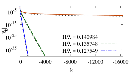
Figure 3: Fig. 3. Spectra of Stokes waves for the values of $H/\lambda$ as in Fig. 2 (thick lines) and fit to (14) with $\beta=1/2$ (thin dashed lines). Solid line shows only a small fraction of the actually numerically resolved spectrum.

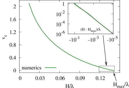
Figure 4: Fig. 4. Position $v_{c}$ of closest singularity of $z(w)$ as a function of $H/\lambda$ obtained numerically. Inset shows zoom-in for $(H_{max}-H)/\lambda\ll 1$ with $H_{max}$ taken from (16) and dashed line is the power law (1).

In summary, we found the Stokes solutions of the primordial Euler equations with free surface for large range of wave heights, including the approach to the limiting Stokes wave. Through the analysis of the solution spectra we calculated in the conformal variables the distance of the lowest singular point in the upper complex half plane to the surface of the fluid as a the function of $H$. We found that this singularity is the square-root branch point. The limiting Stokes wave emerges as the singularity reaches the fluid surface. We found from our high precision simulations the lower bound (15) for the limiting wave of the greatest height $H_{max}$. We also fitted $v_{c}(H)$ to the scaling law (1) which suggests that it might be exactly $\delta=3/2$ as well as it provides the new estimate (16) for $H_{max}.$

The authors would like to thank A. I. Dyachenko for fruitful discussions on application of Petviashvili method to the dynamical equations in conformal variables and D. Appelö for discussion about CG and CR methods. Work of S.D. and A.K. were partially supported by the NSF grant OCE 1131791. Also the authors would like to thank developers of FFTW [34] and the whole GNU project [35] for developing, and supporting this useful and free software.

References

- [1] G. G. Stokes, Transactions of the Cambridge Philosophical Society 8, 441 (1847).
- [2] G. G. Stokes, Mathematical and Physical Papers 1, 197 (1880).
- [3] J. H. Michell, Phil. Mag. Series 5 36, 430 (1893).
- [4] A. I. Nekrasov, Izv. Ivanovo-Voznesensk. Polytech. Inst. 3, 52 (1921).
- [5] A. I. Nekrasov, The exact theory of standing waves on the surface of heavy fluid (Izdat. Akad. Nauk. SSSR, Moscow, 1951).
- [6] L. N. Sretenskii, Theory of wave motion of fluid (Nauka, Moscow, 1976).
- [7] M. A. Grant, J. Fluid Mech. 59(2), 257 (1973).
- [8] L. W. Schwartz, J. Fluid Mech. 62(3), 553 (1974).
- [9] M. S. Longuet-Higgins and M. J. H. Fox, J. Fluid Mech. 80(4), 721 (1977).
- [10] J. M. Williams, Phil. Trans. R. Soc. Lond. A 302(1466), 139 (1981).
- [11] J. M. Williams, Tables of Progressive Gravity Waves (Pitman, London, 1985).
- [12] S. J. Cowley, G. R. Baker, and S. Tanveer, J. Fluid Mech. 378, 233 (1999).
- [13] M. S. Longuet-Higgins, Wave Motion 45, 770 (2008).
- [14] G. R. Baker and C. Xie, J. Fluid Mech. 685, 83 (2011).
- [15] G. G. Stokes, Mathematical and Physical Papers 1, 314 (1880).
- [16] E. A. Kuznetsov, M. D. Spector, and V. E. Zakharov, Phys. Rev. E 49, 1283 (1994).
- [17] A. I. Dyachenko, V. E. Zakharov, and E. A. Kuznetsov, Plasma Physics Reports 22, 829 (1996).
- [18] E. Kuznetsov, M. Spector, and V. Zakharov, Physics Letters A 182, 387 (1993).
- [19] M. Mineev-Weinstein, P. B. Wiegmann, and A. Zabrodin, Physical Review Letters 84, 5106 (2000).
- [20] P. M. Lushnikov, Physics Letters A 329, 49 (2004).
- [21] V. E. Zakharov, A. O. Korotkevich, A. Pushkarev, and D. Resio, Phys. Rev. Lett. 99, 164501 (2007), 0705.2838.
- [22] V. E. Zakharov, A. O. Korotkevich, and A. O. Prokofiev, AIP Proceedings, CP1168 2, 1229 (2009).
- [23] V. E. Zakharov, A. I. Dyachenko, and A. O. Prokofiev, European Journal of Mechanics B/Fluids 25, 677 (2006).
- [24] R. C. T. Rainey and M. S. Longuet-Higgins, Ocean Engineering 33, 2012 (2006).
- [25] L. V. Ovsyannikov, M.A. Lavrent’ev Institute of Hydrodynamics Sib. Branch USSR Ac. Sci. 15, 104 (1973).
- [26] A. I. Dyachenko, E. A. Kuznetsov, M. Spector, and V. E. Zakharov, Phys. Lett. A 221, 73 (1996).
- [27] V. I. Petviashvili, Sov. J. Plasma Phys. 2, 257 (1976).
- [28] P. M. Lushnikov, Opt. Lett. 26, 1535 (2001).
- [29] T. I. Lakoba and J. Yang, J. Comput. Phys. 226, 1668 (2007).
- [30] D.E. Pelinovsky, and Yu.A. Stepanyants, SIAM J. Numer. Anal. 42, 1110 (2004) .
- [31] J. Yang, J Comput. Phys. 228(18), 7007 (2009).
- [32] J. Yang, Nonlinear Waves in Integrable and Nonintegrable Systems (SIAM, 2010).
- [33] D. G. Luenberger, SIAM J. Numer. Anal. 7, 390 (1970).
- [34] M. Frigo and S. G. Johnson, Proc. IEEE 93, 216 (2005).
- [35] G N U Project, http://gnu.org (1984-2013).