Hydrodynamics at RHIC and LHC: What have we learned?

Abstract

Fluid dynamical description of elementary particle collisions has a long history dating back to the works of Landau and Fermi. Nevertheless, it is during the last 10–15 years when fluid dynamics has become the standard tool to describe the evolution of matter created in ultrarelativistic heavy ion collisions. In this review I briefly describe the hydrodynamical models, what we have learned when analyzing the RHIC and LHC data using these models, and what the latest developments and challenges are.

PACS numbers: 25.75Ld, 25.75.Nq, 24.10Nz

1 Introduction

The goal of the heavy-ion programs at BNL RHIC and CERN LHC is to observe strongly interacting matter. ’Strongly interacting’ in a sense that the interactions in the system are not mediated by the electromagnetic, but by the strong interaction, and ’matter’ in the sense that to describe the system, we do not need to describe every (quasi-)particle individually, but thermodynamic concepts like temperature and pressure are applicable. Thus it is natural to try to describe the expansion stage of the collision by a macroscopic approach like fluid dynamics. We expect that the system formed in the collision is initially so hot and dense that relevant degrees of freedom are partons, not hadrons. The system expands and cools, undergoes a phase transition to hadrons, and when the system is dilute enough, interactions cease and the particles stream freely to detectors.

2 Fluid dynamics

2.1 Ideal fluid dynamics

Relativistic fluid dynamics is basically an application of conservation laws for energy, momentum and conserved charges (if any). When written in differential form,

$$\partial_{\mu}T^{\mu\nu}=0,\qquad\mathrm{and}\qquad\partial_{\mu}j_{x}^{\mu}=0,$$ (1)

where $T^{\mu\nu}$ is the energy-momentum tensor, and $j_{x}^{\mu}$ the charge 4-current of charge $x$ (baryon or electric charge, strangeness, isospin,…), the conservation laws provide evolution equations for the system. If there are $n$ conserved charges, there are $4+n$ equations, which contain $10+4n$ unknowns. To make this set of equations solvable, further constraints for the unknowns must be provided. The simplest approach is to assume that the system is in exact local equilibrium. In that case the energy-momentum tensor and charge currents can be expressed as

$$T^{\mu\nu}=(\epsilon+P)u^{\mu}u^{\nu}-Pg^{\mu\nu},\qquad\mathrm{and}\qquad j_{x}^{\mu}=n_{x}u^{\mu},$$ (2)

respectively, where $\epsilon$ and $P$ are energy density and pressure in the local rest frame, $u^{\mu}$ flow velocity, $g^{\mu\nu}$ is the metric tensor, and $n_{x}$ the charge density of charge $x$ in the local rest frame. Now the number of unknowns is reduced to $5+n$, and the system of equations can be closed by providing the equation of state (EoS) of the fluid in a form $P=P(\epsilon,\{n_{i}\})$. To model the collisions at RHIC and LHC, the description is usually further simplified by assuming that net baryon density and other conserved charges are zero. After specifying the boundary conditions for this set of partial differential equations the evolution is determined, and all the microscopic physics is contained within the EoS.

However, the simple phrase “after specifying the boundary conditions” contains a lot of physics. Hydrodynamics provides neither the initial distribution of matter nor the criterion for the end of the evolution, but they must be supplied by other models. At ultrarelativistic energies the initial state of the hydrodynamical evolution cannot be two colliding nuclei: The initial collision processes are far from equilibrium and produce large amount of entropy [3]. Thus the initial state is assumed to be a distribution of thermalized matter soon after the initial collision. The most common approach is so-called Glauber model [4, 5], which is basically a geometrical constraint on the distributions. The Woods-Saxon distributions of nuclear matter in colliding nuclei are projected on a plane orthogonal to the beam (so called transverse plane), and the resulting densities on this plane, and nucleon-nucleon cross section at the collision energy, are used to calculate the number density of binary collisions and participants on this plane—participant meaning a nucleon which has interacted at least once (for details, see Ref. Miller:2007ri). The initial energy or entropy density profile is taken to be proportional to the profile of collisions or participants, or to a linear combination of them [6, 7]. The proportionality constant is a free parameter chosen to reproduce the observed final particle multiplicity.

Another popular approach is the KLN (Kharzeev-Levin-Nardi) model [8, 9, 10, 11, 12, 13] where the initial entropy density distribution is proportional to the distribution of gluons produced in primary collisions. The gluon production is calculated using the Color Glass Condensate (CGC) framework [14, 15, 16, 17], where one applies the feature of QCD that at small-x gluon densities are large. These large densities correspond to classical fields permitting calculations using classical techniques. Another approach to calculate the initial particle production from first principles is so-called EKRT saturation model [18, 19, 20] based on perturbative QCD + saturation framework. Besides these approaches, one can use event generators like UrQMD [22, 23, 21], AMPT [24, 25], or EPOS [26] to generate the initial state for hydrodynamic expansion. Nevertheless, no model so far describes a dynamical process leading to thermalized matter, but thermalization has to be postulated and imposed by hand.

When the system expands and cools, the mean free paths increase. Ultimately mean free paths become so long that rescatterings cease, and particle distributions no longer evolve. Particle distributions are ’frozen’ at that stage, and we say that the particles freeze out, or alternatively, that the particles decouple from each other. In practice this freeze-out should be a gradual process, but since implementing a gradual freeze-out is difficult, it is approximated to take place suddenly on a surface of zero thickness. In such a case one can use so-called Cooper-Frye prescription to evaluate particle distributions on this surface [29]:

$$E\frac{\mathrm{d}N}{\mathrm{d}p^{3}}=\int_{\sigma}\mathrm{d}\sigma_{\mu}p^{\mu}f(T(x),\mu(x),p\cdot u(x)),$$ (3)

where $\sigma$ is the surface where the distribution is to be evaluated, $\mathrm{d}\sigma_{\mu}$ its normal 4–vector, $f$ distribution of particles, and $u$ 4–flow velocity of the fluid. Hydrodynamics does not tell when decoupling should take place, but the criterion is a free parameter, and its value is chosen to reproduce the observed $p_{T}$-spectra. Usually a constant temperature or energy density is used as the criterion, although a more realistic criterion would be the ratio of the scattering rate of particles to the expansion rate of the system, i.e., the inverse Knudsen number [30, 31]

2.2 Dissipative fluid dynamics

The ideal fluid assumption is extremely strong, and in nature gradients in the system always indicate deviations from equilibrium and thus dissipation. In non-relativistic fluid dynamics Navier-Stokes equations are known to describe viscous fluid well, but unfortunately the relativistic generalization of Navier-Stokes equations is unstable and allows acausal solutions with superluminal signal propagation speeds [32, 33, 34]. This undesired behavior can be avoided if one assumes that the dissipative currents (shear stress $\pi^{\mu\nu}$, heat flow $q^{\mu}$ and bulk pressure $\Pi$) are not directly proportional to gradients in the system, but are dynamical variables which relax to their Navier-Stokes values on time scales given by corresponding relaxation times $\tau_{\pi}$, $\tau_{q}$ and $\tau_{\Pi}$. The evolution equations for the dissipative currents can be derived phenomenologically from entropy current [35, 36], from kinetic theory using the Grad 14–moment ansatz [37, 38, 39], or via gradient expansion [40, 41].

The derivation from kinetic theory leads to the commonly used Israel-Stewart equations, but so far it has had a problem: Unlike Chapman-Enskog expansion [42], which leads to relativistic Navier-Stokes equations, it is not a controlled expansion in some small parameter, in which one could do power counting and improve the approximation if necessary. This problem has recently been solved by rederiving viscous hydrodynamics using the method of moments, and ordering the terms in the expansion according to their (generalized) Reynolds and Knudsen numbers [43]. In lowest order in Knudsen and Reynolds numbers this approach leads to equations identical to the original Israel-Stewart approach, but it has been shown that an adequate description of heat flow would require inclusion of some higher order terms[44].

Strictly speaking all these derivations are for a single component system, and the derivation for a multi-component system has not been completed yet [45, 46, 47]. For the behavior of the fluid this does not matter—the different components are assumed to behave as a single fluid—but when the fluid is converted to various types of hadrons, this causes an additional uncertainty. The Cooper-Frye prescription (Eq. (3)) is equally valid in dissipative as in ideal system, but dissipation causes the distribution function $f$ to deviate slightly from the thermal equilibrium distribution. If there is only shear, no bulk pressure nor heat flow, in a single component system the Grad 14–moment ansatz leads in Boltzmann approximation to

$$f=f_{0}+\delta f,\qquad\mathrm{where}\qquad\delta f=f_{0}\frac{p^{\mu}p^{\nu}\pi_{\mu\nu}}{2T^{2}(\epsilon+P)},$$ (4)

and $f_{0}$ is the equilibrium distribution function. In a multicomponent system the effect of shear stress on particle distributions should depend on particle properties, but how exactly, is still a work in progress [48]. In practical calculations one has therefore assumed that the dissipative correction to the thermal distribution is given by Eq. (4) for all hadron species. Note that the form of $\delta f$ in Eq. (4) is only an ansatz. Other forms have been argued for [49], but if the thermal distribution is expanded differently than in the 14–moment ansatz, the evolution equations and definitions of the dissipative coefficients may change as well.

So far the viscous hydrodynamical calculations have concentrated on studying the effects of shear viscosity, characterized by the shear viscosity coefficient $\eta$. In no calculation has heat conductivity been included, and the bulk pressure has usually been omitted as well. When the only dissipative current is shear stress, the energy-momentum tensor becomes

$$T^{\mu\nu}=(\epsilon+P)u^{\mu}u^{\nu}-Pg^{\mu\nu}+\pi^{\mu\nu},$$ (5)

where $\pi^{\mu\nu}$ is the shear stress tensor. Its evolution is usually given by

$$\langle D\pi^{\mu\nu}\rangle=\frac{1}{\tau_{\pi}}\left(2\eta\sigma^{\mu\nu}-\pi^{\mu\nu}\right)-\frac{4}{3}\pi^{\mu\nu}\partial_{\lambda}u^{\lambda},$$ (6)

where $D=u^{\mu}\partial_{\mu}$, $\sigma^{\mu\nu}=\nabla^{\langle\mu}u^{\nu\rangle}$, and the angular brackets $\langle\,\rangle$ denote the symmetrized and traceless projection, orthogonal to the fluid four-velocity $u^{\mu}$. Both Israel-Stewart [39, 43] and gradient expansion [40, 41] approaches lead to some additional terms in the evolution equation, but these terms are usually considered numerically insignificant, although a full analysis of the effect of all terms has not yet been done. It is worth noting that the factor 4/3 in the last term of Eq. (6) is strictly valid for massless particles. Whether modifying this term according to the mass of particles would change any results has not been studied yet. As well, in the original Israel-Stewart papers [36, 38] this term was estimated small and omitted in the final equations. In the context of heavy-ion collisions, however, it improves the applicability of viscous hydrodynamics significantly [55].

2.3 Hybrid models

The sudden change from interacting fluid to free streaming particles in the Cooper-Frye description is clearly an oversimplification. We also expect hadron gas to be so dissipative [45, 56] that the applicability of dissipative fluid dynamics is questionable [57]. In so-called hybrid models these problems are avoided by using fluid dynamics to describe only the early dense stage of the evolution. The fluid is converted to particles using the Cooper-Frye description, not at freeze-out, but when rescatterings are still abundant, and the individual particles are fed to a hadron cascade model like UrQMD [22, 23] or JAM [58, 59] to describe the dilute hadronic stage. These models have the advantage that hadron cascades describe freeze-out dynamically without free parameters, all dissipative processes are included, and they can describe a system arbitrarily far from equilibrium. Unfortunately they do not remove all the arbitrariness from the end of the evolution: Like the results of pure hydrodynamical models depend on the freeze-out criterion, the results of hybrid models depend on when the switch from fluid to cascade is done [57, 60]. For a detailed discussion of these models see Ref. Hirano:2012kj.

3 What we know

3.1 There are rescatterings

Figure 1: A schematic representation of the geometry of a non-central heavy-ion collision. (left:) Two Lorentz-contracted nuclei approaching each other. (right:) A projection of the collision zone onto a plane orthogonal to the beam (so called transverse plane). The dotted circles depict the target and projectile nuclei.

The particle production in the primary collisions is azimuthally isotropic, but the distribution of observed particles in A+A collisions is not. The anisotropy can be easily explained in terms of rescatterings of the produced particles: In a non-central collision of identical nuclei the collision zone has an elongated shape, see Fig. 1. If a particle is moving along the long axis of the collision zone, it has a larger probability to scatter and change its direction than a particle moving along the short axis. Thus more particles end up in the direction of the short axis. Or, in the hydrodynamical language, the pressure gradient between the center of the system and the vacuum is larger in the direction of the short axis, the flow velocity is thus larger in that direction, and more particles are emitted along the short than along the long axis.

This anisotropy is quantified in terms of Fourier expansion of the azimuthal distribution. The coefficients of this expansion $v_{n}$, and the associated participant angles $\psi_{n}$, are defined as

$$v_{n}=\langle\cos[n(\phi-\psi_{n})]\rangle,\qquad\mathrm{and}\qquad\psi_{n}=\frac{1}{n}\arctan\frac{\langle p_{T}\sin(n\phi)\rangle}{\langle p_{T}\cos(n\phi)\rangle}.$$ (7)

Of these coefficients $v_{1}$ is called directed, and $v_{2}$ elliptic flow. Elliptic flow of charged hadrons as a function of centrality was one of the first measurements at RHIC [62]. The result is shown in Fig. 3, and compared to early fluid dynamical calculations [63]. As seen, the elliptic flow is quite large and increases with decreasing centrality, as expected if it has the described geometric origin. Thus there must be rescatterings among the particles formed in the collision, and an A+A collision is not just a sum of independent $pp$ collisions.

The observed elliptic flow is also very close to the hydrodynamically calculated one, which is a strong indication of hydrodynamical behavior of the matter. Another signature of hydrodynamical behavior is shown in Fig. 3: It was observed that the heavier the particle, the smaller its $p_{T}$-differential $v_{2}$ at low $p_{T}$. As explained in Refs. Ollitrault:2007du and Huovinen:2001cy, such a behavior arises if all the particles are emitted from the same expanding thermal source. Thus, if the produced matter is not close to kinetic equilibrium, at least it behaves as if it was!

Figure 2: The elliptic flow parameter $v_{2}$ of charged hadrons as function of centrality ($\mathrm{N_{ch}/N_{max}}=1$ is the most central collision) in Au+Au collisions at $\sqrt{s_{\mathrm{NN}}}=130$ GeV. The data are from Ref. Ackermann:2000tr and the calculation using different EoSs (labels A and H), and freeze-out temperatures (120 MeV or 140 MeV) from Ref. Kolb:2000fha. The figure is from Ref. confinement.

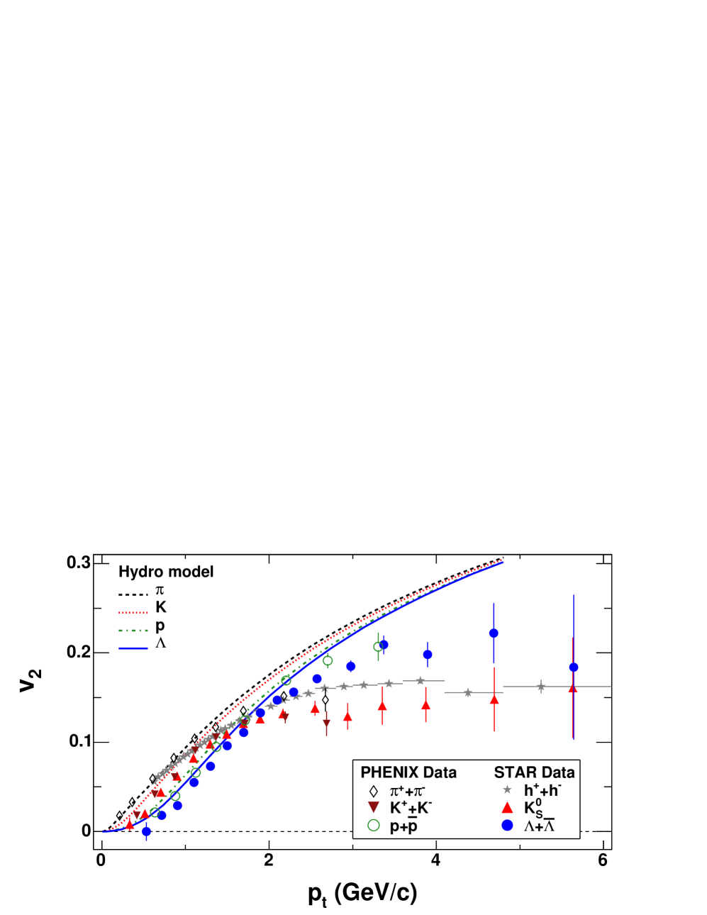
Figure 3: $v_{2}$ vs. $p_{T}$ for identified particles in minimum bias $Au+Au$ collisions at $\sqrt{s_{\mathrm{NN}}}=200$ GeV. The data are from Refs. Adams:2004bi,Adler:2003kt and Adams:2003am. Reprinted figure with permission from Ref. Adams:2004bi. Copyright (2005) by the American Physical Society.

It has often been argued that the large observed $v_{2}$ and its hydrodynamical reproduction requires that the system reaches thermal equilibrium very fast [69], within 1 fm/$c$ after the initial collision. The hydrodynamical models fitting the data do indeed use short initial times, $\tau_{0}=0.15$-1 fm/$c$, but in Ref. Luzum:2008cw it was shown that $\tau_{0}=2$ fm/$c$ works as well. The crucial distinction is what the shape of the initial state is: The larger the deformation, the larger the final momentum anisotropy. During thermalization the matter will not stay put, but begins to expand. This expansion reduces the spatial anisotropy, and unless momentum anisotropy is built up during thermalization, the final anisotropy is smaller [71]. If thermalization is fast, we may assume that changes in matter distribution and flow field during thermalization are tiny, and geometry (Glauber) and/or initial gluon production (Color Glass, EKRT) give reasonable constraints to the initial state of hydrodynamical evolution. In Ref. Luzum:2008cw the shape of the initial state was assumed to be independent of the thermalization time, but if thermalization time is long, this is no longer a good approximation. Thus, if thermalization is fast, we know that we can reproduce the data using hydrodynamical models, but if thermalization takes long, we do not know, since we do not know a plausible initial state for hydrodynamical evolution.

3.2 Equation of State has many degrees of freedom

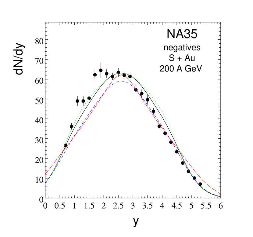
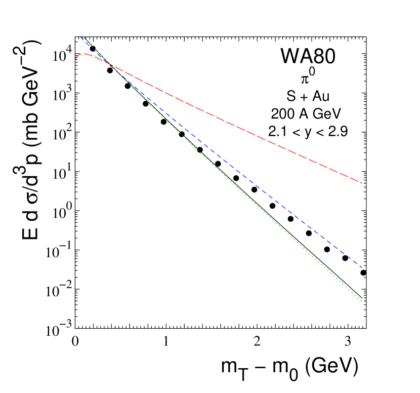
Figure 4: Rapidity distribution of negative hadrons (left) and transverse momentum distribution of neutral pions (right) in S+Au collision at $E_{\mathrm{lab}}=200A$ GeV using four different EoSs. The red long dashed curve corresponds to ideal pion gas EoS, whereas the other curves correspond to hadron resonance gas with or without phase transition to ideal parton gas. The figures are from Ref. Sollfrank:1996hd, and the data from Refs. Gazdzicki:1995cr and Santo:1993ri.

The equation of state (EoS) of strongly interacting matter is an explicit input to hydrodynamical models. Thus one might expect hydrodynamical modeling of heavy-ion collisions to tell us a lot about the EoS, but unfortunately that is not the case. The collective motion of the system is directly affected by the pressure gradients in the system, and thus by the EoS, but the effects of the EoS on the final particle $p_{T}$ distributions can to very large extent be compensated by changes in the initial state of the evolution, and the final decoupling temperature. This makes constraining the properties of the EoS very difficult. However, what we do know is that the number of degrees of freedom has to be large.

It was already seen when modeling S+Au collisions at the CERN SPS at $E_{\mathrm{lab}}=200A$ GeV energy, that if we use ideal pion gas EoS, it is not possible to fit the pion rapidity and $p_{T}$-distributions simultaneously. Once the initial state and decoupling temperature are fixed to reproduce the rapidity distribution, the transverse momentum distribution of pions becomes too flat [72], see Fig. 4. Or if one chooses parameters to fit the $p_{T}$-spectrum, the rapidity distribution is not reproduced. On the other hand, if we use an EoS containing several hadrons and resonances, the distributions can be fitted.

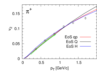
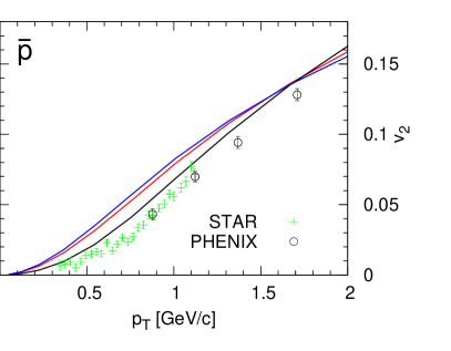
Figure 5: Elliptic flow of pions and antiprotons vs. transverse momentum in minimum bias Au+Au collisions at $\sqrt{s_{\mathrm{NN}}}=200$ GeV calculated using three different EoSs [75] and compared with the data by the STAR and PHENIX collaborations [65, 66]. The labels stand for a lattice QCD inspired quasiparticle model (qp), EoS with a first order phase transition (Q), and pure hadron resonance gas with no phase transition (H). Figure is from Ref. confinement.

One might want to use the elliptic flow to constrain the EoS after the initial state and freeze-out temperature are fixed to reproduce the $p_{T}$ distributions. Unfortunately elliptic flow is only very weakly sensitive to the details of the EoS [75]: The only flow observable affected by the EoS seems to be the $p_{T}$-differential anisotropy of heavy particles, e.g., protons. As shown in Fig. 5, the $v_{2}(p_{t})$ of pions is unchanged within the experimental errors no matter whether one uses an EoS with (EoS A) or without phase transition (EoS H), or an EoS with a first order phase transition (EoS A) or with a smooth crossover (EoS qp). On the other hand, the proton $v_{2}(p_{t})$ is sensitive to the EoS, but surprisingly the EoS with the first order phase transition is closest to the data. Consequently distinguishing between different lattice QCD EoS parametrizations is very difficult, see Ref. Huovinen:2009yb.

3.3 Softest point of the Equation of State is quite hard

The two-particle correlations at low relative momentum provide information about the space-time structure of the source, and thus constraints to dynamical models generating the source. For bosons these correlations are called Bose-Einstein correlations, and for identical particles the method for their interpretation is called Hanbury Brown–Twiss (HBT) interferometry, or, as in general case, femtoscopy [77, 78, 79]. To make the measured/calculated three-dimensional correlator easier to understand, it is often expressed in terms of multi-dimensional Gaussian parametrization, widths of which are called HBT radii. Reproduction of the HBT radii measured at RHIC was surprisingly difficult, and for many years it was not possible to describe simultaneously the particle spectra, their anisotropies, and HBT radii. An inconsistency referred to as “HBT puzzle” [80, 81]. It turned out that this inconsistency was due to several small effects. Successful reproduction of the data required that, 1) the transverse collective expansion begins very early, 2) the EoS is quite hard, 3) dissipative effects are included, and 4) contribution from resonance decays is included [80, 81, 82, 83]. When these requirements are taken into account, the present calculations provide an acceptable fit to the data [26, 52, 84].

The early build up of collective expansion supports the notion of early thermalization discussed in Sec. 3.1, but the HBT radii provide as ambiguous support as elliptic flow. If sufficient collective motion is build up during thermalization, HBT radii can be fitted also if thermalization takes long (so-called pre-equilibrium flow) [80, 81, 83]. The sufficient hardness of the EoS is fortunately more solid requirement. In practice it means that a bag model EoS with a mixed phase, where the speed of sound is negligible, is disfavored, and thus the softest point of the EoS can hardly be any softer than that of hadron resonance gas [85]. A notion in line with the lattice QCD EoS calculations [86].

Nevertheless, since it is so difficult to constrain the EoS, in the present calculations the lattice QCD EoS [86, 87, 88, 89] is taken as given, and the main interest is in studying the dissipative properties of the system. At low temperatures the lattice EoS is equivalent to the EoS of noninteracting hadron resonance gas (HRG) with all the hadrons and resonances in the Particle Data Book up to $\sim 2$–2.5 GeV mass. In calculations one often uses an EoS which is a HRG EoS at low temperature, and connected smoothly to a parametrized lattice EoS at high temperature [76, 90].

In the long run a systematic study of collisions at different energies may reveal some sensitivity to EoS and thus allow to test experimentally the lattice QCD prediction. However, since the parameter space and the amount of data to be fitted are vast, such a study requires the use of model emulators to map the parameter space instead of using actual hydrodynamical model to calculate results at all parameter combinations [91, 92].

3.4 Shear viscosity over entropy density ratio has very low minimum

Once it became clear that ideal fluid dynamics can describe the particle spectra and their anisotropies quite well, it was reasonable to assume that the shear viscosity coefficient over entropy density ratio $\eta/s$ of the matter produced in the collision was very low. But how low in particular? To answer that required the development and use of relativistic dissipative hydrodynamics. Of the other dissipative quantities heat conductivity can be ignored since at midrapidity the matter formed in the collisions at RHIC and LHC is almost baryon free. Thus there is no gradient of chemical potential and no force causing heat flow. The bulk viscosity, on the other hand, is expected to peak around the phase transition, but be small above it. If it is small at lower temperatures too, the effect of bulk viscosity has been evaluated to be smaller than the effect of shear viscosity [51]. Large viscosity in hadronic phase can have a sizable effect [50, 53, 54] but since bulk viscosity in hadron gas is not well known, and there is no reliable method to distinguish the effects of bulk from the effects of shear, the former is largely ignored, and the calculations concentrate on studying the effects of shear viscosity and on extracting the $\eta/s$ ratio from the experimental data [93].

It has been shown that the shear viscosity strongly reduces $v_{2}$ [94]. Thus in principle extracting the $\eta/s$ ratio from the data is easy: One needs to calculate the $p_{T}$-averaged $v_{2}$ of charged hadrons using various values of $\eta/s$ and choose the value of $\eta/s$ which reproduces the data. Unfortunately this approach is hampered by our ignorance of the initial state of the evolution. Fig. 6 shows a viscous fluid calculation of $v_{2}$ of charged hadrons from the first attempt to extract $\eta/s$ from the data. As seen, a curve corresponding to a finite value of $\eta/s$ fits the data best, but the preferred value depends on how the initial state of hydrodynamic evolution is chosen: Whether one uses Glauber [4] or KLN approach [10, 12] (see sect. 2.1) causes a factor two difference in the preferred value ($\eta/s=0.08$–0.16). Furthermore, the approximations in the description of the late hadron gas stage in these calculations caused additional uncertainties, so it was estimated [96] that based on these results $\eta/s<5/(4\pi)$.

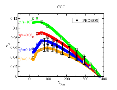
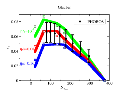
Figure 6: Charged hadron $v_{2}$ as function of centrality in Au+Au collisions at $\sqrt{s_{\mathrm{NN}}}=200$ GeV using different values of $\eta/s$ and KLN (labeled CGC, left) or Glauber (right) initial conditions. The larger the number of participants, $N_{\mathrm{part}}$, the more central the collision. The data are from Ref. Alver:2007zz. Reprinted figures with permission from Ref. Luzum:2008cw. Copyright (2008) by the American Physical Society.

The description of hadronic stage in Ref. Luzum:2008cw was problematic for two reasons. It assumed chemical equilibrium until the very end of the evolution, but at RHIC, the final particle yields correspond to a chemically equilibrated source in $T=160$–165 MeV temperature [97, 98]. The decoupling temperature required to fit the $p_{T}$-distributions is usually around $T_{\mathrm{dec}}=100$–140 MeV. Thus there must be a stage where the fluid is in local kinetic, but not in chemical equilibrium. Such a “chemically frozen” stage turned out to have surprisingly large effect on the collective flow in general and elliptic flow in particular [99, 100]. The second problem was that $\eta/s$ was constant during the entire evolution, but the theoretical expectation is that hadron gas has much larger viscosity than what the obtained value $\eta/s=0.08$–0.16 indicates [45, 56].

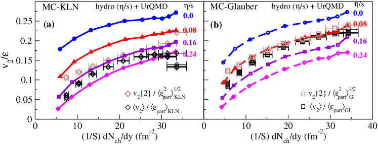
Figure 7: $v_{2}$ scaled by the initial state anisotropy $\epsilon$, $v_{2}/\epsilon$, as function of centrality, characterized by the final multiplicity per area of the initial state, $(1/S)\,\mathrm{d}N/\mathrm{d}y$, in Au+Au collisions at $\sqrt{s_{\mathrm{NN}}}=200$ GeV. The experimental data are from Refs. Ollitrault:2009ie, Adams:2004bi and Abelev:2008ab for $\langle v_{2}\rangle$, $v_{2}\{2\}$, and $\mathrm{d}N_{\mathrm{ch}}/\mathrm{d}y$, respectively. The experimental data used in (a) and (b) are identical, but the normalization factors $\langle\varepsilon_{\mathrm{part}}\rangle$, $\langle\varepsilon_{\mathrm{part}}^{2}\rangle^{1/2}$ and $S$ are taken from the MC-KLN model in (a) and from the MC-Glauber model in (b). The viscous hydro + UrQMD hadron cascade hybrid model calculations from Ref. Song:2010mg are done using the MC-KLN initial conditions in (a) and MC-Glauber in (b). Reprinted figure with permission form Ref. Song:2010mg. Copyright (2011) by the American Physical Society.

In subsequent calculations these uncertainties have been addressed. A state-of-the-art calculation of Ref. Song:2010mg employs a hybrid viscous hydro + UrQMD hadron cascade model. Such a model reduces the uncertainty related to the description of hadron gas since it provides a dynamical description of chemistry and dissipative properties—including bulk viscosity—based on the scattering cross sections of various hadron species. Unfortunately some uncertainties still remain: It is uncertain whether hadron cascade is applicable in the vicinity of phase transition where the switch from hydro to cascade is done, the dissipative properties of the system (i.e. $\eta$, $\zeta$, $\tau_{\pi}$ and $\tau_{\Pi}$) change abruptly at the switch, and the results also depend on when the switch from hydro to cascade is done [57]. The elliptic flow coefficient $v_{2}$ as function of centrality as calculated in Ref. Song:2010mg is shown in Fig. 7. In this figure the coefficients $v_{2}$ have been scaled by the anisotropy of the initial shape, $\epsilon$, and consequently the resulting $v_{2}/\epsilon$ is almost independent of the initialization. Unfortunately $\epsilon$ is not a measurable, but a model dependent quantity. Thus the data has to be scaled by the same $\epsilon$ which was used in the calculation, and the data points in Fig. 7 depend on the model used to initialize the calculation. The result is almost identical to the one shown in Fig. 6—Glauber initialization favors lower value of viscosity, $\eta/s\approx 0.08$, than KLN initialization, $\eta/s\approx 0.16$. Since the uncertainties are smaller, this result was estimated to provide a limit $1/(4\pi)<\eta/s<2.5/(4\pi)$ for the effective QGP viscosity [96, 101]. For further discussion of evaluating $\eta/s$, see Ref. Song:2012tv.

4 What we are working with

4.1 $\eta/s(T)$

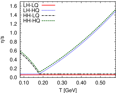
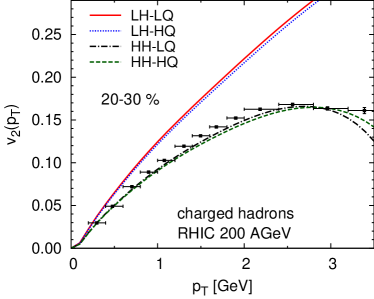
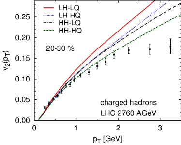
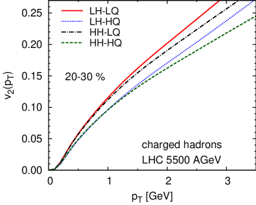
Figure 8: (top left:) Different parametrizations of $\eta/s$ as a function of temperature. The (LH-LQ) line is shifted downwards and the (HH-HQ) line upwards for clarity. Labels refer to low (L) or high (H) viscosity in the hadronic (H) or partonic (Q) phases. (top right:) $v_{2}(p_{T})$ of charged hadrons in the 20-30% Au+Au collisions at $\sqrt{s_{\mathrm{NN}}}=200$ GeV (RHIC). Data are from Refs Bai,Tang:2008if. (bottom left:) $v_{2}(p_{T})$ of charged hadrons in the 20-30% Pb+Pb collisions at $\sqrt{s_{\mathrm{NN}}}=2.76$ TeV (LHC). Data are from Ref Lissu. (bottom right:) $v_{2}(p_{T})$ of charged hadrons in the 20-30% Pb+Pb collisions at $\sqrt{s_{\mathrm{NN}}}=5.5$ TeV (LHC). All the figures are from Ref. sQM.

Calculations discussed in section 3.4 assumed that the $\eta/s$-ratio is constant. We know no fluid where $\eta/s$ would be temperature independent, and there are theoretical reasons to expect it to depend on temperature with a minimum around the phase transition [104]. Thus the temperature independent $\eta/s$ is an effective viscosity, and its connection to the physical, temperature dependent, shear viscosity coefficient is unclear. What complicates the determination of the physical shear viscosity coefficient, is that the sensitivity of the anisotropies to dissipation varies during the evolution of the system. As studied in Ref. Harri, and illustrated in Fig. 8, at RHIC ($\sqrt{s_{\mathrm{NN}}}=200$ GeV) $v_{2}(p_{T})$ is insensitive to the value of $\eta/s$ above phase transition, but very sensitive to its value in the hadronic phase. At the present LHC energy ($\sqrt{s_{\mathrm{NN}}}=2.76$ TeV) the shear viscosity in the plasma phase does affect the final $v_{2}(p_{T})$, but not more than the shear viscosity in the hadronic phase. It is only at the full LHC energy, $\sqrt{s_{\mathrm{NN}}}=5.5$ TeV where the viscosity in the plasma phase dominates, and dissipation in the hadronic phase has only a minor effect. Note that a change of the minimum value of $\eta/s$ would clearly change $v_{2}(p_{T})$ at all energies.

Figure 9: (left:) Parametrizations of $\eta/s$ as a function of temperature with different minima. The (HH-HQ) line is the same than in Fig. 8. (right:) $v_{2}(p_{t})$ of charged hadrons at RHIC using $\eta/s(T)$ with different minima and different relaxation times. Figures are from Ref. Harri.

Additional factor complicating the determination of the temperature dependence of $\eta/s$ is that the effect of viscosity on the anisotropies does not depend only on the ratio $\eta/s$, but also on the relaxation time $\tau_{\pi}$ of the shear stress tensor. This is demonstrated in Fig. 9. If the minimum value of $\eta/s$ is increased by a factor two, $v_{2}$ is reduced as expected, but if the relaxation time is also increased by a factor two, the effect of the increase in $\eta/s$ is almost completely compensated [105]. The interplay of relaxation time and shear viscosity was discussed also in Refs. Song:2010aq and Shen:2011kn, where it was found that to reproduce hybrid model results using viscous hydrodynamics only, it is not sufficient to increase $\eta/s$ in the hadronic phase, but one should also change the relaxation time.

So far we have seen that calculations with constant $\eta/s$ require slightly larger value of $\eta/s$ at LHC than at RHIC [112, 111]. This is in line with the increase of $(\eta/s)(T)$ in high temperatures, but as shown in Ref. Song:2011qa, one cannot uniquely constrain $(\eta/s)(T)$ by fitting the spectra and $v_{2}$ alone.

4.2 Fluctuations

Figure 10: An example of the positions of interacting nuclei in MC-Glauber model. Figure is from Ref. Hannu.

Figure 11: Ratio of the anisotropy coefficients of charged hadrons in viscous calculation to the coefficients in ideal fluid calculation [117]. Figure shown in Ref. [64] by courtesy of Björn Schenke.

In the average the matter formed in heavy-ion collisions has a smooth shape as indicated in Fig. 1, but in each event that is not true. Nuclei are not smooth distributions of nuclear matter, but consist of individual nucleons, and thus the collision zone can be expected to have a highly irregular shape which fluctuates event-by-event, see Fig. 11. The initial state models (see sect. 2.1) can be generalized to so-called Monte-Carlo (MC) models to take this into account. In those models the initial Woods-Saxon distributions of nuclear matter are sampled to generate configurations of nucleons in nuclei, and the number of participants/collisions [4] or gluon production [12, 13] in an event is calculated based on the positions of individual nuclei.

It was shown already a while ago that the final observables differ whether one first averages the initial state, and evolves it hydrodynamically, or one evolves the event-by-event fluctuating initial states individually, and averages the results [114, 115]. This became widely recognized only years later when it was realized that because of the irregular shape of each event, not only even, but also odd anisotropy coefficients $v_{n}$ are finite and measurable [116]. The higher coefficients are very helpful for extracting the transport coefficients from the data, since the larger the $n$, the more sensitive the coefficient $v_{n}$ is to viscosity [117], see Fig. 11. Thus the study of fluctuations provides a way to distinguish different initializations, and first results for the $p_{T}$-dependence of $v_{2}$ and $v_{3}$ (called triangular flow) seem to favor the MC-Glauber initialization [118].

It has been suggested that initial fluctuations provide also a way to circumvent our ignorance of the initial shape [119]. In most central collisions the anisotropies are entirely driven by fluctuations, which are better understood than the average shape in semi-central collisions. Thus evaluating $\eta/s$ using $v_{n}$ in the most central collisions should be less sensitive to the model used to calculate the initial state. The preliminary result of such an analysis was that $0.07<\eta/s<0.43$ [119]. This value is again for effective viscosity which does not exclude the possibility that $\eta/s$ could be even smaller or larger in some temperature region. For a further discussion of flow and viscosity, see Ref. Heinz:2013th.

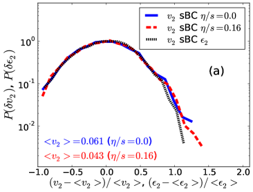
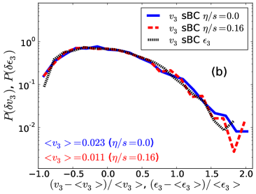
Figure 12: Probability distributions: a) P($\delta v_{2}$) and P($\delta\epsilon_{2}$), and b) P($\delta v_{3}$) and P($\delta\epsilon_{3}$ ) in the 20 − 30 % centrality class with sBC Glauber model initialization and two different values of $\eta/s$, $\eta/s=0$ and $\eta/s=0.16$. $\delta v_{n}=(v_{n}-\langle v_{n}\rangle)/\langle v_{n}\rangle$ and $\delta\epsilon_{n}=(\epsilon_{n}-\langle\epsilon_{n}\rangle)/\langle\epsilon_{n}\rangle$. Figures are from Ref. [120].

In event-by-event studies it is not sufficient to reproduce only the average values of $v_{n}$, but the fluctuations of the flow coefficients should be reproduced as well. The distributions of these fluctuations provide a way to constrain the fluctuation spectrum of initial state models independently of the dissipative properties of the fluid. As shown in Fig. 12, once the average $v_{n}$ has been scaled out, the distributions of these fluctuations, i.e., $(v_{n}-\langle v_{n}\rangle)/\langle v_{n}\rangle$ or $v_{n}/\langle v_{n}\rangle$, are almost independent of viscosity. The independence extends to other details of the evolution to such an extent, that the distributions of the fluctuations of initial anisotropies are good approximations of the measured distributions of $v_{n}$ [120], and thus it is sufficient to compare the fluctuations of initial shape, $\epsilon_{n}$, to the observed fluctuations of $v_{n}$. Unlike the recently developed IP-Glasma model [121, 122], neither MC-Glauber nor MC-KLN model seems to be able to reproduce the measured fluctuations [123].

4.3 Initialization

During last two years there have been major advances in modeling the initial state of hydrodynamical evolution. So called IP-Glasma model [121, 122] is based on Color Glass Condensate and employs the IP-Sat (Impact Parameter dependent Saturation) model [124, 125] of nucleon wavefunctions to generate fluctuating gluon fields in the initial collision, and the classical Yang-Mills dynamics to evolve these fields [126, 127, 128, 129, 130, 131]. Unlike most of the initial state models, the IP-Glasma model includes the fluctuations of color charge in colliding nucleons too, not only the fluctuations of nucleon positions. Another advantage is that the model includes some of the pre-equilibrium dynamics of the gluon fields making the model less sensitive on the time when one switches to hydrodynamics [111]. Unfortunately the description is still incomplete: the present IP-Glasma model does not lead to a thermal system, but final thermalization still has to be assumed. Nevertheless, calculations using the IP-Glasma initialization reproduce both the fluctuations and the average values of $v_{2}$, $v_{3}$ and $v_{4}$ [111, 132], which makes this approach very promising. For a general overview of IP-Glasma, fluctuations and hydrodynamics, see Ref. Gale:2013da.

5 What worries us

As described in the previous sections, fluid dynamics has been very successful in describing heavy ion collisions. However, at the time of this writing there are some data which may cause difficulties for the conventional fluid dynamical picture.

5.1 Photons

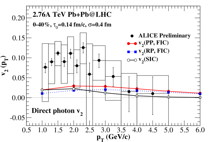
Figure 13: Thermal photon $v_{2}$ vs. $p_{T}$ for 0–40% central collisions at LHC. The preliminary direct photon data are from Ref. Lohner:2012ct. Reprinted figure with permission from Ref. Chatterjee:2013naa. Copyright (2013) by the American Physical Society.

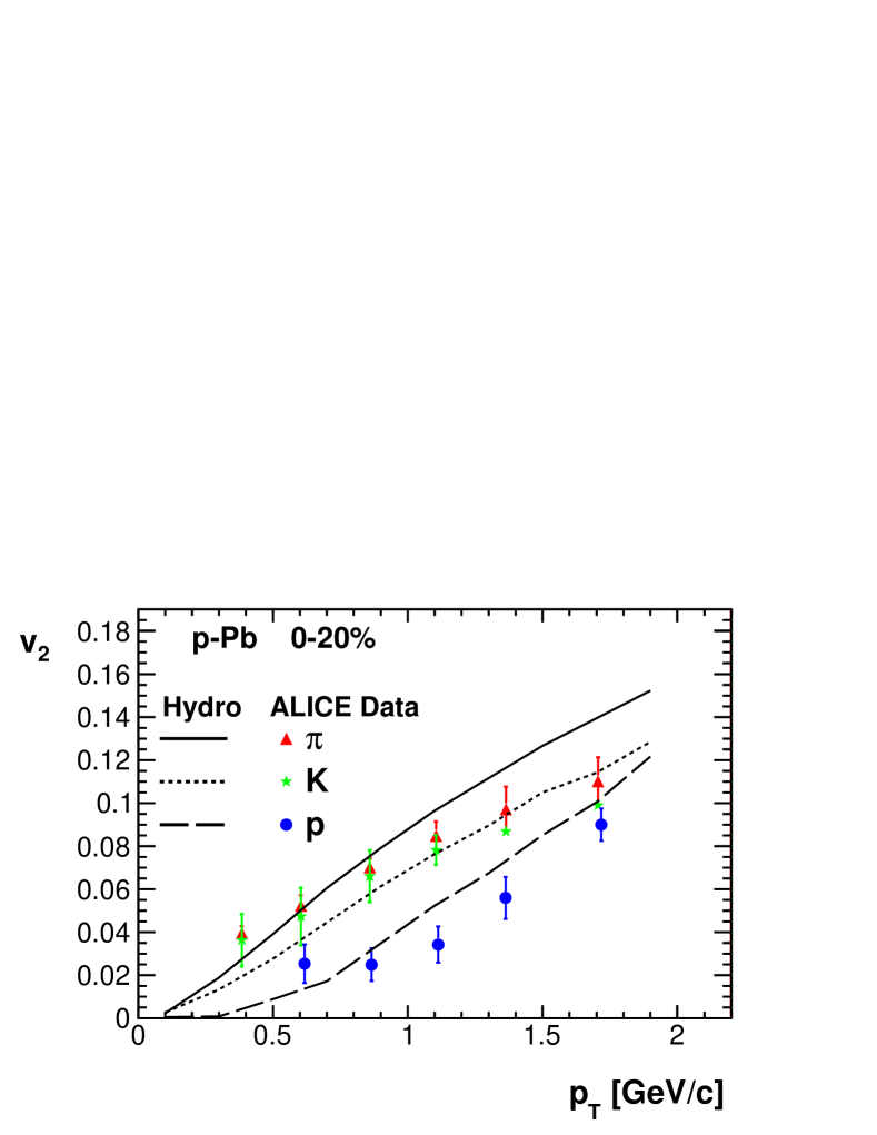
Figure 14: $v_{2}$ vs. $p_{T}$ for identified particles in 0–20% most central $p+Pb$ collisions. Data are from Ref. ABELEV:2013 and the hydrodynamical calculation from Ref. Bozek:2013ska. Figure courtesy by Piotr Bozek.

Unlike hadrons and partons, photons and leptons interact only electromagnetically, and hardly scatter at all after being produced. Thus the observed photon and lepton spectra contain contributions from all stages of a heavy-ion collision, and can be used to probe the early hot and dense stage [134]. The yield and $p_{T}$-spectrum of photons in heavy-ion collisions is fairly well understood [135, 136, 137, 138, 139] —see also Ref. Gale:2012xq and references therein—but the recent measurements of direct photon $v_{2}$ at RHIC [141] and LHC [142] have presented a puzzle: If photons are emitted during all stages of the evolution, and momentum anisotropy increases during the evolution, photon $v_{2}$ should be smaller than the hadron $v_{2}$. Such a behavior is seen in the theoretical calculations [143], but not in the data where the photon $v_{2}(p_{T})$ is roughly equal to the observed pion $v_{2}(p_{T})$ [141, 142]. The further refinements of the calculations, where event-by-event fluctuations [144] and viscosity have been taken into account [145, 146], have not been able to increase the $v_{2}$ to the observed level, see Fig. 14. So far the only approach to get close to the data has used parametrized expansion with very strong initial expansion and large photon production rates in the hadronic phase [147]. Thus the reproduction of the data remains a challenge to our understanding of microscopic production rates and/or expansion dynamics.

5.2 $p+Pb$ collisions

In $p+Pb$ collisions at $\sqrt{s_{\mathrm{NN}}}=5.02$ TeV, the measured dihadron correlations [148, 149, 150, 151], multiplicity and species dependence of average $p_{T}$ [152, 153], and elliptic and triangular flows [149, 150, 151] all depict features easily explained by using hydrodynamics [154, 155, 156, 157, 158, 159] (For a short summary see Ref. Bozek:2013yfa). Especially striking is the mass ordering of the $p_{T}$-differential elliptic flow [151], see Fig. 14. As discussed in section 3.1, this was taken as a strong indicator of the formation of a thermal system. However, it is questionable whether hydrodynamics is applicable to such a small system. Gradients are so large, that dissipative corrections should be of the same order than equilibrium pressure. As discussed in Ref. Bzdak:2013zma, large dissipative corrections are a problem even in $Pb+Pb$ collisions, but in $Pb+Pb$ collisions corrections are large only for a small fraction of the lifetime of the system, whereas corrections are large for a significant fraction of the lifetime in $p+Pb$ collision.

In the Color Glass Condensate framework similar correlations [162, 163, 164] and the mass hierarchy of average $p_{T}$ [165] arise as a result of gluon saturation in the proton and nuclear wavefunctions. How much of the observed behavior can be explained as such an initial state effect, and how to differentiate initial state effects from hydrodynamical final state effects [161, 166] is at the time of this writing under intense study. If it turns out that the apparently hydrodynamical behavior in $p+Pb$ collisions can be explained as an initial state effect, then we may wonder whether the hydrodynamical behavior in $Pb+Pb$ collisions could be explained as an initial state effect as well. On the other hand, if this is not possible, and fluid dynamics is the most viable description of $p+Pb$ collisions, then the properties of QCD matter are even more surprising than thought so far.

6 Summary

Fluid dynamics has been very successful in explaining the features of bulk, i.e. low $p_{T}$, particle production in ultrarelativistic heavy-ion collisions. We have seen that in particular anisotropies of particle production can be explained if the rescatterings among particles are so frequent that the system is approximately thermal, that the equation of state of such a matter has many degrees of freedom and relatively hard, and that the shear viscosity coefficient over entropy ratio of the produced matter has very low value at some temperature. Providing further experimental constraints on the equation of state as well as figuring out the temperature dependence and the precise value of the minimum of $\eta/s$ will require a lot of work. The present studies in event-by-event fluctuations and recent advances in modeling the pre-equilibrium processes in heavy-ion collisions are very helpful for this goal, but it is not yet clear how the elliptic flow of photons in $A+A$ collisions and the $p+Pb$ collisions at LHC fit in the overall picture. After a few years’ work we will know.

References

- [1] D. H. Rischke, arXiv:nucl-th/9809044.
- [2] J.-Y. Ollitrault, Eur. J. Phys. 29 (2008) 275.
- [3] B. Muller and A. Schafer, Int. J. Mod. Phys. E 20 (2011) 2235.
- [4] M. L. Miller, K. Reygers, S. J. Sanders and P. Steinberg, Ann. Rev. Nucl. Part. Sci. 57 (2007) 205.
- [5] A. Bialas, M. Bleszynski and W. Czyz, Nucl. Phys. B 111 (1976) 461.
- [6] P. F. Kolb et al., Nucl. Phys. A 696 (2001) 197.
- [7] U. W. Heinz and P. F. Kolb, Nucl. Phys. A 702 (2002) 269.
- [8] D. Kharzeev and M. Nardi, Phys. Lett. B 507 (2001) 121.
- [9] D. Kharzeev and E. Levin, Phys. Lett. B 523 (2001) 79.
- [10] D. Kharzeev, E. Levin and M. Nardi, Phys. Rev. C 71 (2005) 054903.
- [11] D. Kharzeev, E. Levin and M. Nardi, Nucl. Phys. A 730 (2004) 448 [Erratum-ibid. A 743 (2004) 329].
- [12] H.-J. Drescher and Y. Nara, Phys. Rev. C 75 (2007) 034905.
- [13] H. -J. Drescher and Y. Nara, Phys. Rev. C 76 (2007) 041903.
- [14] E. Iancu, A. Leonidov and L. McLerran, arXiv:hep-ph/0202270.
- [15] E. Iancu and R. Venugopalan, in Quark-Gluon Plasma 3, eds. R. C. Hwa and X.-N. Wang (World Scientific, Singapore, 2004), p. 249.
- [16] F. Gelis, E. Iancu, J. Jalilian-Marian and R. Venugopalan, Ann. Rev. Nucl. Part. Sci. 60 (2010) 463.
- [17] T. Lappi, Int. J. Mod. Phys. E 20 (2011) 1.
- [18] K. J. Eskola, K. Kajantie, P. V. Ruuskanen and K. Tuominen, Nucl. Phys. B 570 (2000) 379.
- [19] R. Paatelainen, K. J. Eskola, H. Holopainen and K. Tuominen, Phys. Rev. C 87 (2013) 044904.
- [20] R. Paatelainen, K. J. Eskola, H. Niemi and K. Tuominen, arXiv:1310.3105 [hep-ph].
- [21] H. Petersen et al., Phys. Rev. C 78 (2008) 044901.
- [22] S. A. Bass et al., Prog. Part. Nucl. Phys. 41 (1998) 255.
- [23] M. Bleicher et al., J. Phys. G 25 (1999) 1859.
- [24] B. Zhang, C. M. Ko, B.-A. Li and Z.-W. Lin, Phys. Rev. C 61 (2000) 067901.
- [25] L. Pang, Q. Wang and X.-N. Wang, Phys. Rev. C 86 (2012) 024911.
- [26] K. Werner et al., Phys. Rev. C 82 (2010) 044904.
- [27] S. V. Akkelin, Y. Hama, I. A. Karpenko and Y. M. Sinyukov, Phys. Rev. C 78 (2008) 034906.
- [28] I. A. Karpenko and Y. M. Sinyukov, Phys. Rev. C 81 (2010) 054903.
- [29] F. Cooper and G. Frye, Phys. Rev. D 10 (1974) 186.
- [30] J. P. Bondorf, S. I. A. Garpman and J. Zimanyi, Nucl. Phys. A 296, (1978) 320.
- [31] H. Holopainen and P. Huovinen, J. Phys. Conf. Ser. 389 (2012) 012018.
- [32] W. A. Hiscock and L. Lindblom, Annals Phys. 151 (1983) 466.
- [33] W. A. Hiscock and L. Lindblom, Phys. Rev. D 31 (1985) 725.
- [34] W. A. Hiscock and L. Lindblom, Phys. Rev. D 35 (1987) 3723.
- [35] I. Muller, Z. Phys. 198 (1967) 329.
- [36] W. Israel, Annals Phys. 100 (1976) 310.
- [37] H. Grad, Commun. Pure Appl. Math. 2 (1949) 331.
- [38] W. Israel and J. M. Stewart, Annals Phys. 118 (1979) 341.
- [39] G. S. Denicol, E. Molnar, H. Niemi and D. H. Rischke, Eur. Phys. J. A, 48 11 (2012) 170.
- [40] R. Baier et al., JHEP 0804 (2008) 100.
- [41] P. Romatschke, Class. Quant. Grav. 27 (2010) 025006.
- [42] S. Chapman and T. G. Cowling, The mathematical theory of non-uniform gases, 3rd edition (Cambridge University Press, Cambridge, 1970).
- [43] G. S. Denicol, H. Niemi, E. Molnar and D. H. Rischke, Phys. Rev. D 85 (2012) 114047.
- [44] G. S. Denicol et al., arXiv:1207.6811 [nucl-th].
- [45] M. Prakash, M. Prakash, R. Venugopalan and G. Welke, Phys. Rept. 227 (1993) 321.
- [46] A. Monnai and T. Hirano, Nucl. Phys. A 847 (2010) 283.
- [47] G. S. Denicol and H. Niemi, Nucl. Phys. A 904-905 (2013) 369c.
- [48] D. Molnar, J. Phys. G 38 (2011) 124173.
- [49] K. Dusling, G. D. Moore and D. Teaney, Phys. Rev. C 81, (2010) 034907.
- [50] A. Monnai and T. Hirano, Phys. Rev. C 80 (2009) 054906.
- [51] H. Song and U. W. Heinz, Phys. Rev. C 81 (2010) 024905.
- [52] P. Bozek, Phys. Rev. C 85 (2012) 034901.
- [53] K. Dusling and T. Schäfer, Phys. Rev. C 85 (2012) 044909.
- [54] J. Noronha-Hostler et al., Phys. Rev. C 88 (2013) 044916.
- [55] P. Huovinen and D. Molnar, Phys. Rev. C 79 (2009) 014906.
- [56] N. Demir and S. A. Bass, Phys. Rev. Lett. 102 (2009) 172302.
- [57] H. Song, S. A. Bass and U. Heinz, Phys. Rev. C 83 (2011) 024912.
- [58] Y. Nara et al., Phys. Rev. C 61 (2000) 024901.
- [59] M. Isse et al., Phys. Rev. C 72 (2005) 064908.
- [60] T. Hirano, P. Huovinen, K. Murase and Y. Nara, Prog. Part. Nucl. Phys. 70 (2013) 108.
- [61] S. A. Voloshin, A. M. Poskanzer and R. Snellings, arXiv:0809.2949 [nucl-ex].
- [62] K. H. Ackermann et al. [STAR Collaboration], Phys. Rev. Lett. 86 (2001) 402.
- [63] P. F. Kolb, P. Huovinen, U. W. Heinz and H. Heiselberg, Phys. Lett. B 500 (2001) 232.
- [64] P. Huovinen, PoS ConfinementX, (2012) 165.
- [65] J. Adams et al. [STAR Collaboration], Phys. Rev. C 72 (2005) 014904.
- [66] S. S. Adler et al. [PHENIX Collaboration], Phys. Rev. Lett. 91 (2003) 182301.
- [67] J. Adams et al. [STAR Collaboration], Phys. Rev. Lett. 92 (2004) 052302.
- [68] P. Huovinen et al., Phys. Lett. B 503 (2001) 58.
- [69] P. F. Kolb and U. W. Heinz, in Quark-Gluon Plasma 3, eds. R. C. Hwa and X.-N. Wang (World Scientific, Singapore, 2004), p. 634.
- [70] M. Luzum and P. Romatschke, Phys. Rev. C 78 (2008) 034915 [Erratum-ibid. C 79 (2009) 039903].
- [71] P. F. Kolb, J. Sollfrank and U. W. Heinz, Phys. Rev. C 62 (2000) 054909.
- [72] J. Sollfrank et al., Phys. Rev. C 55 (1997) 392.
- [73] M. Gazdzicki et al. [NA35 Collaboration], Nucl. Phys. A 590 (1995) 197C.
- [74] R. Santo et al. [WA80 Collaboration], Nucl. Phys. A 566 (1994) 61C.
- [75] P. Huovinen, Nucl. Phys. A 761 (2005) 296.
- [76] P. Huovinen and P. Petreczky, Nucl. Phys. A 837 (2010) 26.
- [77] M. A. Lisa, S. Pratt, R. Soltz and U. Wiedemann, Ann. Rev. Nucl. Part. Sci. 55 (2005) 357.
- [78] M. A. Lisa and S. Pratt, arXiv:0811.1352 [nucl-ex].
- [79] M. A. Lisa et al., New J. Phys. 13 (2011) 065006.
- [80] S. Pratt, Phys. Rev. Lett. 102 (2009) 232301.
- [81] S. Pratt, Nucl. Phys. A 830 (2009) 51C.
- [82] A. Kisiel, W. Florkowski and W. Broniowski, Phys. Rev. C 73 (2006) 064902.
- [83] W. Broniowski, M. Chojnacki, W. Florkowski and A. Kisiel, Phys. Rev. Lett. 101 (2008) 022301.
- [84] I. A. Karpenko, Y. M. Sinyukov and K. Werner, Phys. Rev. C 87 (2013) 024914.
- [85] M. Chojnacki and W. Florkowski, Acta Phys. Polon. B 38 (2007) 3249.
- [86] S. Borsanyi et al., JHEP 1011 (2010) 077.
- [87] O. Philipsen, Prog. Part. Nucl. Phys. 70 (2013) 55.
- [88] P. Petreczky, J. Phys. G 39 (2012) 093002.
- [89] S. Borsanyi et al., arXiv:1309.5258 [hep-lat].
- [90] M. Bluhm et al., arXiv:1306.6188 [hep-ph].
- [91] H. Petersen, C. Coleman-Smith, S. A. Bass and R. Wolpert, J. Phys. G 38 (2011) 045102.
- [92] J. Novak et al., arXiv:1303.5769 [nucl-th].
- [93] U. W. Heinz and R. Snellings, Annu. Rev. Nucl. Part. Sci. 63 (2013) 123.
- [94] D. Teaney, Phys. Rev. C 68 (2003) 034913.
- [95] B. Alver [PHOBOS Collaboration], Int. J. Mod. Phys. E 16 (2007) 3331.
- [96] H. Song, Eur. Phys. J. A 48 (2012) 163.
- [97] A. Andronic, P. Braun-Munzinger and J. Stachel, Phys. Lett. B 673 (2009) 142 [Erratum-ibid. B 678 (2009) 516].
- [98] A. Andronic, P. Braun-Munzinger and J. Stachel, Acta Phys. Polon. B 40 (2009) 1005.
- [99] T. Hirano and K. Tsuda, Phys. Rev. C 66 (2002) 054905.
- [100] P. Huovinen, Eur. Phys. J. A 37 (2008) 121.
- [101] H. Song et al., Phys. Rev. Lett. 106 (2011) 192301 [Erratum-ibid. 109 (2012) 139904].
- [102] J. Y. Ollitrault, A. M. Poskanzer and S. A. Voloshin, Phys. Rev. C 80, (2009) 014904.
- [103] B. I. Abelev et al. [STAR collaboration], Phys. Rev. C 79, (2009) 034909.
- [104] L. P. Csernai, J. I. Kapusta, L. D. McLerran, Phys. Rev. Lett. 97, (2006) 152303.
- [105] H. Niemi et al., Phys. Rev. C 86 (2012) 014909.
- [106] Y. Bai, Ph.D. Thesis, Nikhef and Utrecht University, Utrecht (2007).
- [107] A. Tang [STAR Collaboration], arXiv:0808.2144 [nucl-ex].
- [108] K. Aamodt et al. [ALICE Collaboration], Phys. Rev. Lett. 105, (2011) 252302.
- [109] H. Niemi et al., Acta Phys. Polon. Supp. 5 (2012) 305.
- [110] C. Shen and U. Heinz, Phys. Rev. C 83 (2011) 044909.
- [111] C. Gale et al., Phys. Rev. Lett. 110 (2013) 012302.
- [112] H. Song, S. A. Bass and U. Heinz, Phys. Rev. C 83 (2011) 054912 [Erratum-ibid. C 87 (2013) 019902].
-
[113]
H. Holopainen,
Ph.D. Thesis, University of Jyväskylä, Jyväskylä (2011).
http://urn.fi/URN:ISBN:978-951-39-4371-4 - [114] C. E. Aguiar, Y. Hama, T. Kodama and T. Osada, Nucl. Phys. A 698 (2002) 639.
- [115] O. Socolowski, Jr., F. Grassi, Y. Hama and T. Kodama, Phys. Rev. Lett. 93 (2004) 182301.
- [116] B. Alver and G. Roland, Phys. Rev. C 81 (2010) 054905 [Erratum-ibid. C 82 (2010) 039903].
- [117] B. Schenke, S. Jeon and C. Gale, Phys. Rev. C 85 (2012) 024901.
- [118] Z. Qiu, C. Shen and U. Heinz, Phys. Lett. B 707 (2012) 151.
- [119] M. Luzum and J.-Y. Ollitrault, Nucl. Phys. A 904-905 (2013) 377c.
- [120] H. Niemi, G. S. Denicol, H. Holopainen and P. Huovinen, Phys. Rev. C 87 (2013) 054901.
- [121] B. Schenke, P. Tribedy and R. Venugopalan, Phys. Rev. Lett. 108 (2012) 252301.
- [122] B. Schenke, P. Tribedy and R. Venugopalan, Phys. Rev. C 86 (2012) 034908.
- [123] J. Jia [ATLAS Collaboration], Nucl. Phys. A 904-905 (2013) 421c.
- [124] J. Bartels, K. J. Golec-Biernat and H. Kowalski, Phys. Rev. D 66 (2002) 014001.
- [125] H. Kowalski and D. Teaney, Phys. Rev. D 68 (2003) 114005.
- [126] A. Kovner, L. D. McLerran and H. Weigert, Phys. Rev. D 52 (1995) 6231.
- [127] Y. V. Kovchegov and D. H. Rischke, Phys. Rev. C 56 (1997) 1084.
- [128] A. Krasnitz and R. Venugopalan, Nucl. Phys. B 557 (1999) 237.
- [129] A. Krasnitz and R. Venugopalan, Phys. Rev. Lett. 84 (2000) 4309.
- [130] A. Krasnitz and R. Venugopalan, Phys. Rev. Lett. 86 (2001) 1717.
- [131] T. Lappi, Phys. Rev. C 67 (2003) 054903.
- [132] C. Gale et al., Nucl. Phys. A 904-905 (2013) 409c.
- [133] C. Gale, S. Jeon and B. Schenke, Int. J. Mod. Phys. A 28 (2013) 1340011.
- [134] K. Kajantie and H. I. Miettinen, Z. Phys. C 9 (1981) 341.
- [135] S. Turbide, C. Gale, S. Jeon and G. D. Moore, Phys. Rev. C 72 (2005) 014906.
- [136] S. Turbide, C. Gale, E. Frodermann and U. Heinz, Phys. Rev. C 77 (2008) 024909.
- [137] R. Chatterjee and D. K. Srivastava, Phys. Rev. C 79 (2009) 021901.
- [138] R. Chatterjee, H. Holopainen, T. Renk and K. J. Eskola, Phys. Rev. C 83 (2011) 054908.
- [139] H. Holopainen, S. Rasanen and K. J. Eskola, Phys. Rev. C 84 (2011) 064903.
- [140] C. Gale, Nucl. Phys. A 910-911 (2013) 147.
- [141] A. Adare et al. [PHENIX Collaboration], Phys. Rev. Lett. 109 (2012) 122302.
- [142] D. Lohner [ALICE Collaboration], J. Phys. Conf. Ser. 446 (2013) 012028.
- [143] R. Chatterjee, E. S. Frodermann, U. W. Heinz and D. K. Srivastava, Phys. Rev. Lett. 96 (2006) 202302.
- [144] R. Chatterjee et al., Phys. Rev. C 88 (2013) 034901.
- [145] M. Dion et al., Phys. Rev. C 84 (2011) 064901.
- [146] C. Shen et al., arXiv:1308.2111 [nucl-th].
- [147] H. van Hees, C. Gale and R. Rapp, Phys. Rev. C 84 (2011) 054906.
- [148] B. Abelev et al. [ALICE Collaboration], Phys. Lett. B 719 (2013) 29.
- [149] S. Chatrchyan et al. [CMS Collaboration], Phys. Lett. B 724 (2013) 213.
- [150] G. Aad et al. [ATLAS Collaboration], Phys. Lett. B 725 (2013) 60.
- [151] B. B. Abelev et al. [ALICE Collaboration], Phys. Lett. B 726 (2013) 164.
- [152] B. B. Abelev et al. [ALICE Collaboration], arXiv:1307.1094 [nucl-ex].
- [153] S. Chatrchyan et al. [CMS Collaboration], arXiv:1307.3442 [hep-ex].
- [154] P. Bozek and W. Broniowski, Phys. Lett. B 718 (2013) 1557.
- [155] P. Bozek and W. Broniowski, Phys. Rev. C 88 (2013) 014903.
- [156] T. Pierog et al., arXiv:1306.0121 [hep-ph].
- [157] G.-Y. Qin and B. Müller, arXiv:1306.3439 [nucl-th].
- [158] K. Werner et al. arXiv:1307.4379 [nucl-th].
- [159] P. Bozek, W. Broniowski and G. Torrieri, Phys. Rev. Lett. 111 (2013) 172303.
- [160] P. Bozek, W. Broniowski and G. Torrieri, arXiv:1309.7782 [nucl-th].
- [161] A. Bzdak, B. Schenke, P. Tribedy and R. Venugopalan, Phys. Rev. C 87 (2013) 064906.
- [162] K. Dusling, F. Gelis, T. Lappi and R. Venugopalan, Nucl. Phys. A 836 (2010) 159.
- [163] K. Dusling and R. Venugopalan, Phys. Rev. D 87 (2013) 094034.
- [164] K. Dusling and R. Venugopalan, Phys. Rev. D 87 (2013) 054014.
- [165] L. McLerran, M. Praszalowicz and B. Schenke, Nucl. Phys. A 916 (2013) 210.
- [166] P. Bozek, A. Bzdak and V. Skokov, arXiv:1309.7358 [hep-ph].