B-1348 Louvain-la-Neuve, Belgium 22institutetext: Theoretische Natuurkunde and IIHE/ELEM, Vrije Universiteit Brussel, and International Solvay Institutes,
Pleinlaan 2, B-1050 Brussels, Belgium 33institutetext: LPTHE, CNRS UMR 7589, UPMC Univ. Paris 6, Paris 75252, France
Higgs characterisation via vector-boson fusion and associated production: NLO and parton-shower effects
Abstract
Vector-boson fusion and associated production at the LHC can provide key information on the strength and structure of the Higgs couplings to the Standard Model particles. Using an effective field theory approach, we study the effects of next-to-leading order (NLO) QCD corrections matched to parton shower on selected observables for various spin-0 hypotheses. We find that inclusion of NLO corrections is needed to reduce the theoretical uncertainties on total rates as well as to reliably predict the shapes of the distributions. Our results are obtained in a fully automatic way via FeynRules and MadGraph5_aMC@NLO.
1 Introduction
After the discovery of a new boson at the LHC Aad:2012tfa ; Chatrchyan:2012ufa , studies of its properties have become the first priority of the high energy physics community. A coordinated theoretical and experimental effort is in place Dittmaier:2011ti ; Dittmaier:2012vm ; Heinemeyer:2013tqa that aims at maximising the information from the ongoing and forthcoming measurements. On the experimental side, new analyses, strategies and more precise measurements are being performed that cover the wider range of relevant production and decay channels in the Standard Model (SM) and beyond, and the recent measurements of the coupling strength ATLAS:2013sla ; Chatrchyan:2013lba and the spin-parity properties Aad:2013xqa ; Chatrchyan:2012jja give strong indication that the new particle is indeed the scalar boson predicted by the SM. On the theoretical side, predictions for signal and background are being obtained at higher orders in perturbative expansion in QCD and electroweak (EW), so that a better accuracy in the extraction of the SM parameters can be achieved. In addition, new variables and observables are being proposed that can be sensitive to new physics effects. At the same time, considerable attention is being devoted to the definition of a theoretical methodology and framework to collect and interpret the constraints coming from the experimental side.
The proposal of employing an effective field theory (EFT) that features only SM particles and symmetries at the EW scale has turned out to be particularly appealing. Such a minimal assumption, certainly well justified by the present data, provides not only a drastic reduction of all possible interactions that Lorentz symmetry alone would allow, but also a well-defined and powerful framework where constraints coming from Higgs measurements can be globally analysed together with those coming from precision EW measurements and flavor physics (see for example refs. Hagiwara:1993qt ; Giudice:2007fh ; Gripaios:2009pe ; Lafaye:2009vr ; Low:2009di ; Morrissey:2009tf ; Contino:2010mh ; Espinosa:2010vn ; Azatov:2012bz ; Espinosa:2012ir ; Ellis:2012rx ; Klute:2012pu ; Low:2012rj ; Corbett:2012dm ; Ellis:2012hz ; Montull:2012ik ; Espinosa:2012im ; Carmi:2012in ; Plehn:2012iz ; Passarino:2012cb ; Corbett:2012ja ; Cheung:2013kla ; Falkowski:2013dza ; Contino:2013kra ; Chen:2013ejz , and more in general refs. Buchmuller:1985jz ; Grzadkowski:2010es ).
In this context, the Higgs Characterisation (HC) framework has been recently presented Artoisenet:2013puc that follows the general strategy outlined in ref. Christensen:2009jx . A simple EFT lagrangian featuring bosons with various spin-parity assignments has been implemented in FeynRules Christensen:2008py ; Alloul:2013bka and passed to the MadGraph5_aMC@NLO Alwall:2011uj ; Frederix:2009yq ; Hirschi:2011pa framework by means of the UFO model file Degrande:2011ua ; deAquino:2011ub . Such an implementation is simple but general enough to describe any new physics effects coming from higher scales in a fully model-independent way. It has the advantage of being systematically and seamlessly improvable through the inclusion of more operators in the lagrangian on one side and of higher-order corrections, notably those coming from QCD, on the other. The latter, considered in the form of multi-parton tree-level computations (ME+PS) and of next-to-leading order (NLO) calculations matched to parton showers (NLO+PS), are a very important ingredient for performing sensible phenomenological studies.
In ref. Artoisenet:2013puc we have provided a study of higher order QCD effects for inclusive production, with , , , and , and correlated decay of resonances into a pair of gauge bosons, where gluon fusion ( annihilation) is dominant for spin-0 and spin-2 (spin-1) at the LO. In this work, we present the results for the next most important production channels at the LHC, i.e., weak vector-boson fusion (VBF) and associated production (VH), focusing on the most likely spin-0 hypothesis. As already noted in ref. Artoisenet:2013puc , these processes share the property that NLO QCD corrections factorise exactly with respect to the new physics interactions in Higgs couplings and therefore can be automatically performed within the current MadGraph5_aMC@NLO framework. Given that the Higgs characterisation can also be done automatically in production channel Frederix:2011zi , all the main Higgs production channels are covered.
We stress that the spin-parity studies in VBF and VH production nicely complement those in decays Hagiwara:2009wt ; Englert:2012xt . One of the advantages in the VBF and VH channels is that spin-parity observables, e.g., the azimuthal difference between the two tagging jets in VBF, do not require a reconstruction of the Higgs resonance, although the separation between the and contributions is very difficult. In this study, we focus on the effects of the QCD corrections in Higgs VBF and VH production without considering the decay.
The paper is organised as follows. In the following section we recall the relevant effective lagrangian of ref. Artoisenet:2013puc , and define the sample scenarios used to illustrate the phenomenological implications. In sect. 3 we present the VBF results in the form of distributions of key observables in the inclusive setup as well as with dedicated VBF cuts, while in sect. 4 we illustrate the and production. We briefly summarise our findings in the concluding section.
2 Theoretical setup
In this section, we summarise the full setup, from the lagrangian, to the choice of benchmark scenarios, to event generation at NLO accuracy.
2.1 Effective lagrangian and benchmark scenarios
We construct an effective lagrangian below the electroweak symmetry breaking (EWSB) scale in terms of mass eigenstates. Our assumptions are simply that the resonance structure observed in data corresponds to one bosonic state ( with , , or , and a mass of about GeV), and that no other new state below the cutoff coupled to such a resonance exists. We also follow the principle that any new physics is dominantly described by the lowest dimensional operators. This means, for the spin-0 case, that we include all effects coming from the complete set of dimension-six operators with respect to the SM gauge symmetry.
| parameter | description |
|---|---|
| [GeV] | cutoff scale |
| ) | mixing between and |
| dimensionless coupling parameter |
| 0 |
The effective lagrangian relevant for this work, i.e., for the interactions between a spin-0 state and vector bosons, is (eq. (2.4) in ref. Artoisenet:2013puc ):
| (1) |
where the (reduced) field strength tensors are defined as
| (2) | ||||
| (3) |
and the dual tensor is
| (4) |
Our parametrisation: i) allows to recover the SM case easily by the dimensionless coupling parameters and the dimensionful couplings shown in tables 1 and 2; ii) includes state couplings typical of SUSY or of generic two-Higgs-doublet models (2HDM); iii) describes -mixing between and states, parametrised by an angle , in practice .
The corresponding implementation of the dimension-six lagrangian above the EWSB scale, where is an exact symmetry, has recently appeared Alloul:2013naa that has overlapping as well as complementary features with respect to our HC lagrangian. We note that the lagrangian of eq. (1) features 14 free parameters, of which one possibly complex (). On the other hand, as explicitly shown in table 1 of ref. Alloul:2013naa these correspond to 11 free parameters in the parametrisation above the EWSB due to the custodial symmetry. We stress that results at NLO in QCD accuracy shown here can be obtained for that lagrangian in exactly the same way.
| scenario | HC parameter choice |
|---|---|
| (SM) | |
| (HD) | |
| (HDder) | |
| (SM+HD) | |
| (HD) | |
| (HD) |
In table 3 we list the representative scenarios that we later use for illustration. The first corresponds to the SM. The second scenario, (HD), includes only the -even higher dimensional operators corresponding to in a custodial invariant way for VBF. The third scenario, (HDder), includes the so-called derivative operators which, via the equations of motions, can be linked to contact operators of the type . The fourth scenario, (SM+HD), features the interference, which scales as in the physical observables, between the SM and the HD operators. The fifth scenario, (HD), is the analogous of the second one, but for a pseudoscalar. Finally, the sixth scenario, (HD), is representative of a -mixed case, where the scalar is a scalar/pseudoscalar state in equal proportion.
2.2 NLO corrections including parton-shower effects
The MadGraph5_aMC@NLO framework is designed to automatically perform the computation of tree-level and NLO cross sections, possibly including their matching to parton showers and the merging of samples with different parton multiplicities. Currently, the full automation is available in a unique and self-contained framework based on MadGraph5 Alwall:2011uj for SM processes with NLO QCD corrections. User intervention is limited to the input of physics quantities, and after event generation, to the choice of observables to be analysed. In ref. Artoisenet:2013puc results for gluon fusion have been presented and compared to predictions coming from ME+PS (MLM- merging Mangano:2001xp ; Alwall:2007fs ; Alwall:2008qv ) and NLO +PS. Distributions were found compatible between the two predictions. In this work we limit ourselves to NLO+PS results as typical observables are inclusive in terms of extra radiation and such calculations do also provide a reliable normalisation.
aMC@NLO implements matching of any NLO QCD computation with parton showers following the MC@NLO approach Frixione:2002ik . Two independent and modular parts are devoted to the computation of specific contributions to an NLO-matched computation: MadFKS Frederix:2009yq takes care of the Born, the real-emission amplitudes, and it also performs the subtraction of the infrared singularities and the generation of the Monte Carlo subtraction terms, according to the FKS prescription Frixione:1995ms ; Frixione:1997np ; MadLoop Hirschi:2011pa computes the one-loop amplitudes, using the CutTools Ossola:2007ax implementation of the OPP integrand-reduction method Ossola:2006us . The OpenLoops method Cascioli:2011va is also used for better performance. Once the process of interest is specified by the user, the generation of the code is fully automated. Basic information, however, must be available about the model and the interactions of its particles with QCD partons. For MadFKS this amounts to the ordinary Feynman rules. For MadLoop, on the other hand, the Feynman rules, UV counterterms, and special tree-level rules, so-called , necessary to (and defined by) the OPP method, should be provided. While Feynman rules are automatically computed from a given lagrangian (via FeynRules Christensen:2008py ; Alloul:2013bka ), this is not yet possible for UV counterterms and rules. At this moment this limitation hampers the automatic computation of NLO QCD corrections for arbitrary processes in generic BSM models, including the HC model. The processes considered in this paper, VBF and VH, are, however, a notable exception as QCD corrections can be computed automatically and in full generality. This is because the corresponding one-loop amplitudes only include SM particles and do not need any UV counterterms and information from the HC lagrangian. In the case of VBF, this assumes that only vertex loop-corrections can be computed, i.e., the pentagon diagrams are discarded as the contributions only affect interferences between the diagrams, which are negligible already at LO.
2.3 Simulation parameters
In our simulations we generate events at the LHC with a center-of-mass energy TeV and set the resonance mass to GeV. Parton distributions functions (PDFs) are evaluated by using the MSTW2008 (LO/NLO) parametrisation Martin:2009iq , and jets are reconstructed via the anti- () algorithm Cacciari:2008gp as implemented in FastJet Cacciari:2011ma . Central values for the renormalisation and factorisation scales are set to and for VBF and VH production, respectively, where is the invariant mass of the VH system. We note here that scale (and PDF) uncertainties can be evaluated automatically in the code via a reweighting technique Frederix:2011ss , the user only deciding the range of variation. In addition, such information is available on an event-by-event basis and therefore uncertainty bands can be plotted for any observable of interest. In this work, however, to simplify the presentation that focuses on the differences between the various scenarios, we give this information only for total cross sections and refrain from showing them in the differential distributions. For parton shower and hadronisation we employ HERWIG6 Corcella:2000bw in this paper, while HERWIG++ Bahr:2008pv , (virtuality ordered) Pythia6 Sjostrand:2006za and Pythia8 Sjostrand:2007gs are available to use in aMC@NLO, and the comparison among the above different shower schemes was done for the SM Higgs boson in VBF in ref. Frixione:2013mta .
3 Vector boson fusion
Predictions for Higgs production via VBF in the SM are known up to NNLO accuracy for the total cross section Harlander:2008xn ; Bolzoni:2010xr ; Bolzoni:2011cu , at the NLO QCD Han:1992hr ; Figy:2003nv ; Berger:2004pca ; Figy:2004pt ; Hankele:2006ma ; Figy:2010ct + EW Ciccolini:2007jr ; Ciccolini:2007ec level in a differential way and at NLO in QCD plus parton shower both in the POWHEG BOX Nason:2009ai and in aMC@NLO Frixione:2013mta . NLO QCD predictions that include anomalous couplings between the Higgs and a pair of vector bosons are available in VBFNLO Arnold:2008rz ; Arnold:2011wj . Our implementation provides the first predictions for EFT interactions including NLO corrections in QCD interfaced with a parton shower. Many phenomenological studies on Higgs spin, parity and couplings are available in the literature Plehn:2001nj ; Hagiwara:2009wt ; Englert:2012ct ; Andersen:2012kn ; Englert:2012xt ; Djouadi:2013yb ; Englert:2013opa ; Frank:2013gca ; Anderson:2013afp , which could now be upgraded to NLO+PS accuracy.
In our framework the code and events for VBF can be automatically generated by issuing the following commands (note the $$ sign to forbid diagrams with or bosons in the -channel which are included in VH production):
 > import model HC_NLO_X0
 > generate p p > x0 j j $$ w+ w- z QCD=0 [QCD]
 > output
 > launch
As a result all processes featuring a vertex, with are generated, therefore including and . We do not investigate their effects in our illustrative studies below (i.e., we set the corresponding to zero in the simulation), as we focus on SM-like VBF observables. As mentioned above, since our interest is geared towards QCD effects on production distributions, we do not include Higgs decays in our studies either. We stress, however, that decays (as predicted in the HC model) can be efficiently included at the partonic event level (before passing the event to a shower program) via MadSpin Artoisenet:2012st .
| scenario | (fb) | (fb) | |||
|---|---|---|---|---|---|
| (SM) | 1509(1) | 1633(2) | 1.08 | ||
| (HD) | 69.66(6) | 67.08(13) | 0.96 | ||
| (HDder) | 721.9(6) | 684.9(1.5) | 0.95 | ||
| (SM+HD) | 3065(2) | 3144(5) | 1.03 | ||
| (HD) | 57.10(4) | 55.24(11) | 0.97 | ||
| (HD) | 63.46(5) | 61.07(13) | 0.96 |
In table 4, we first collect results for total cross sections at LO and NLO accuracy together with scale uncertainties and corresponding -factors for the six scenarios defined in table 3. We do not impose any cuts here, and hence the cross sections are identical with and without parton shower. The cross sections for the HD hypotheses are calculated with the corresponding set to one and the cutoff scale TeV except for the (SM+HD) scenario, where we set GeV. We do this to allow for visible effects of the interference between the SM and HD terms. Equivalently, we could have kept TeV and chosen a larger value for , as only the ratio is physical. The figures in parentheses give the numerical integration uncertainties in the last digit(s). The other uncertainties correspond to the envelope obtained by varying independently the renormalisation and factorisation scales around the central value with . NLO QCD corrections contribute constructively for the SM case, while destructively for the HD cases, although the global -factors are rather mild. The uncertainty in the HD scenarios, especially for the derivative operator (HDder), are larger than that in the SM case. Manifestly, the uncertainties are significantly reduced going from LO to NLO.
For the studies on the distributions, we require the presence of at least two reconstructed jets with
| (5) |
In addition, we simulate a dedicated VBF selection by imposing an invariant mass cut on the two leading jets,
| (6) |
As well known such a cut has the scope to minimise the contributions from gluon fusion and allow to extract VBF couplings. We note that we do not put the rapidity separation cut, although this is the common VBF cut, since itself is a powerful observable to determine the structure in VBF production Englert:2012xt ; Djouadi:2013yb .
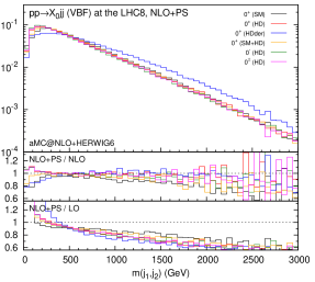
We start by showing the invariant mass distribution of the two leading jets in fig. 1 for the six scenarios of table 3, where the minimal detector cuts in eq. (5) are applied. With the exception of the scenario featuring the derivative operator (HDder), the distributions are all very similar. This means that the invariant mass cut in eq. (6), which is imposed in typical VBF selections, acts in a similar way on all scenarios.
The lowest inset in fig. 1 is the ratio of NLO+PS to LO results, while the middle one shows the ratio of NLO+PS to pure NLO. NLO+PS corrections modify in consistent way LO parton-level predictions with major effects at high invariant mass, i.e., the QCD corrections tend to make the tagging jets softer. In addition, parton shower affects both the lower and higher invariant mass regions.
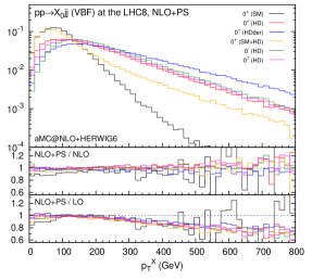
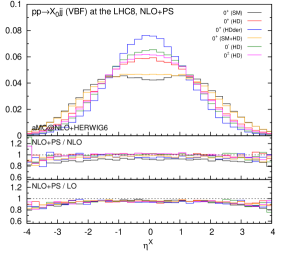
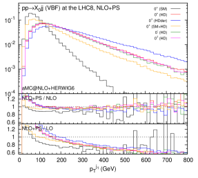
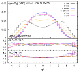
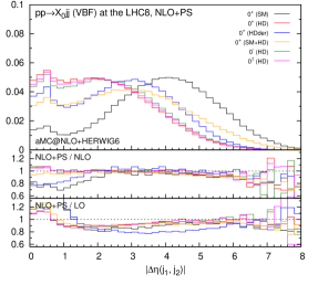
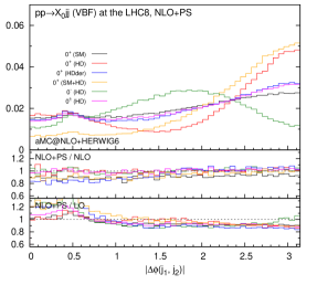

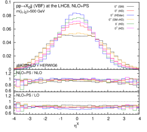
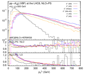
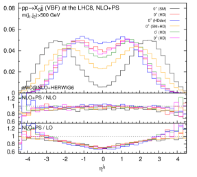
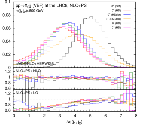
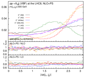
Figures 2 and 3 collect key plots for the and the hardest jet distributions, as well as the rapidity and azimuthal separation of the two leading jets. In fig. 2 only the acceptance cuts in eq. (5) are imposed, while in fig. 3 the additional VBF cut in eq. (6) is applied. As one can see, the invariant mass cut effectively suppresses the central jet activity, especially for the SM case, while the difference of the distributions among the different scenarios becomes more pronounced.
The unitarity violating behaviour of the higher dimensional interactions, especially for (HDder), clearly manifests itself in the transverse momentum distributions for the and the jets. The rapidity distribution of the tagging jets displays the fact that in the case of higher-dimensional interactions the jets result to be much more central than the SM case. Same glaring difference appear in the azimuthal correlations between the jets which offer clear handle to discriminate about different interactions type and parity assignments.
In all cases NLO corrections are relevant and cannot be described by an overall -factor. Moreover, their impact depends on the applied cuts. Apart from regions in phase space where the jets end up close and therefore are sensitive to NLO/jet reconstruction effects, the parton-shower effect on the shapes is very minor, especially after the VBF cut.
4 Vector boson associated production
Predictions for Higgs production in association with a weak vector boson in the SM are known up to NNLO accuracy Brein:2003wg ; Ferrera:2011bk ; Brein:2012ne , including EW corrections Ciccolini:2003jy ; Denner:2011id . NLO+PS results can be obtained via (a)MC@NLO Frixione:2005gz ; LatundeDada:2009rr and the POWHEG BOX Luisoni:2013cuh . Many phenomenological studies on Higgs spin, parity and couplings are available in the literature Miller:2001bi ; Christensen:2010pf ; Desai:2011yj ; Ellis:2012xd ; Englert:2012xt ; Ellis:2013ywa ; Godbole:2013saa ; Isidori:2013cga ; Delaunay:2013npa ; Anderson:2013afp . In this section we present the first predictions for EFT interactions including NLO corrections in QCD interfaced with a parton shower in the VH process.
The code and events for VH production at hadron colliders can be automatically generated by issuing the following commands:
 > import model HC_NLO_X0
 > generate p p > x0 e+ ve [QCD]
 > add process p p > x0 e- ve~ [QCD]
 > add process p p > x0 e+ e- [QCD]
 > output
 > launch
Note that the decays are performed at the level of the matrix elements and therefore all spin correlations are kept exactly. Again, as in sect. 3, we do not consider contributions involving the and vertices.
Results for total cross sections (without any cuts) at LO and NLO accuracy and corresponding -factors for the six scenarios defined in table 3 are collected in tables 5, 6 and 7 for , , and , respectively, including the decay branching ratio into a lepton pair. As in the VBF case, the uncertainties correspond to the envelope of independently varying the renormalisation and factorisation scales around the central value with . Apart from the case of the SM for which the uncertainties are accidentally small at LO, the results at NLO display an improved stability. Quite interestingly all -factors are found to be around 1.3 for all the scenarios, with tiny difference among the processes due to the different initial states. We note that the cancellation of the -channel vector-boson propagator due to the derivative in the higher-dimensional scenarios results in the rather large cross section in spite of the TeV cutoff (except for the (SM+HD) scenario, where GeV).
| scenario | (fb) | (fb) | |||
|---|---|---|---|---|---|
| (SM) | 39.58(3) | 51.22(5) | 1.29 | ||
| (HD) | 13.51(1) | 17.51(1) | 1.30 | ||
| (HDder) | 324.2(2) | 416.1(4) | 1.28 | ||
| (SM+HD) | 118.8(1) | 154.2(1) | 1.30 | ||
| (HD) | 8.386(7) | 10.89(1) | 1.30 | ||
| (HD) | 10.96(1) | 14.22(1) | 1.30 |
| scenario | (fb) | (fb) | |||
|---|---|---|---|---|---|
| (SM) | 22.46(1) | 29.86(3) | 1.33 | ||
| (HD) | 7.009(5) | 9.355(9) | 1.34 | ||
| (HDder) | 145.7(1) | 193.8(1) | 1.33 | ||
| (SM+HD) | 57.90(5) | 77.31(8) | 1.34 | ||
| (HD) | 4.151(3) | 5.550(5) | 1.34 | ||
| (HD) | 5.583(4) | 7.445(7) | 1.33 |
| scenario | (fb) | (fb) | |||
|---|---|---|---|---|---|
| (SM) | 10.13(1) | 13.24(1) | 1.31 | ||
| (HD) | 2.638(2) | 3.461(3) | 1.31 | ||
| (HDder) | 48.61(4) | 63.59(5) | 1.31 | ||
| (SM+HD) | 19.95(1) | 26.24(2) | 1.32 | ||
| (HD) | 1.480(1) | 1.952(1) | 1.32 | ||
| (HD) | 2.061(1) | 2.705(2) | 1.31 |
We then show, fig. 4, distributions for the several inclusive variables with minimal cuts on the charged lepton(s):
| (7) |
for and production (distributions for are very similar to and we do not display them).
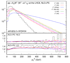
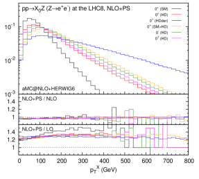
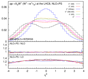
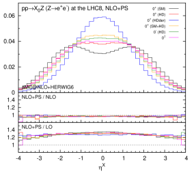
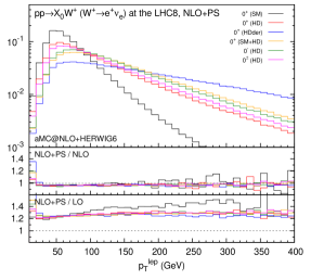
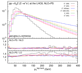
The results for and display very similar features. The scenarios that include contributions from higher dimensional operators show harder spectra. This is even more pronounced in the case of the derivative operator (HDder). This fact is also reflected in the shape of rapidity distributions, i.e., the harder spectra correspond to more central rapidity for the VH scattering.
As in sect. 3, the ratios of NLO+PS to LO (NLO) results are presented in the lowest (middle) inset in fig. 4. NLO+PS effects are quite important when compared with fixed-order LO predictions, and, in many cases, they cannot be accounted for by applying an overall -factor. Conversely, NLO+PS distributions are in almost perfect agreement with fixed-order NLO predictions, witnessing small effects genuinely due to the parton shower.
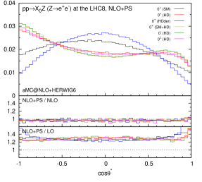
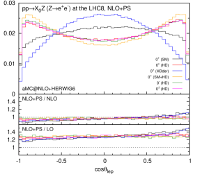
In fig. 5 we show the polar angle distributions in production. is defined as an angle between the intermediate momentum and the reconstructed in the rest frame, while is the lepton angle along the momentum in the rest frame. In this case, NLO+PS corrections do not affect the distributions significantly, while those of are mildly modified. We note that the asymmetry of the distribution is due to the cuts on the leptons.
5 Summary
We have studied higher order QCD effects for various spin-0 hypotheses in VBF and VH production, obtained in a fully automatic way via the model implementation in FeynRules and event generation at NLO accuracy in MadGraph5_aMC@NLO framework. Our approach to Higgs characterisation is based on an EFT that takes into account all relevant operators up to dimension six written in terms of fields above the EWSB scale and then expressed in terms of mass eigenstates (, and ).
We have presented illustrative distributions obtained by interfacing NLO parton-level events to HERWIG6 parton shower. NLO corrections improve the predictions on total cross sections by reducing the scale dependence. In addition, our simulations show that NLO+PS effects need to be accounted for to make accurate predictions on the kinematical distributions of the final state objects, such as the Higgs and the jet distributions.
We look forward to the forthcoming LHC experimental studies employing the EFT approach and NLO accurate simulations to extract accurate information on possible new physics effects in Higgs physics.
Acknowledgments
We would like to thank all the members of Higgs Cross Section Working Group for their encouragement in pursuing the Higgs Characterisation project. We also thank Stefano Frixione for helpful comments on the draft.
This work has been performed in the framework of the ERC grant 291377 “LHCtheory: Theoretical predictions and analyses of LHC physics: advancing the precision frontier” and it is supported in part by the Belgian Federal Science Policy Office through the Interuniversity Attraction Pole P7/37. The work of FM is supported by the IISN “MadGraph” convention 4.4511.10, the IISN “Fundamental interactions” convention 4.4517.08. KM is supported in part by the Strategic Research Program “High Energy Physics” and the Research Council of the Vrije Universiteit Brussel. The work of MZ is partially supported by the Research Executive Agency (REA) of the European Union under the Grant Agreement number PITN-GA-2010-264564 (LHCPhenoNet).
References
- (1) ATLAS Collaboration, G. Aad et al., Observation of a new particle in the search for the Standard Model Higgs boson with the ATLAS detector at the LHC, Phys.Lett. B716 (2012) 1–29, [arXiv:1207.7214].
- (2) CMS Collaboration, S. Chatrchyan et al., Observation of a new boson at a mass of 125 GeV with the CMS experiment at the LHC, Phys.Lett. B716 (2012) 30–61, [arXiv:1207.7235].
- (3) LHC Higgs Cross Section Working Group Collaboration, S. Dittmaier et al., Handbook of LHC Higgs Cross Sections: 1. Inclusive Observables, arXiv:1101.0593.
- (4) LHC Higgs Cross Section Working Group Collaboration, S. Dittmaier et al., Handbook of LHC Higgs Cross Sections: 2. Differential Distributions, arXiv:1201.3084.
- (5) LHC Higgs Cross Section Working Group Collaboration, S. Heinemeyer et al., Handbook of LHC Higgs Cross Sections: 3. Higgs Properties, arXiv:1307.1347.
- (6) ATLAS Collaboration, Combined coupling measurements of the Higgs-like boson with the ATLAS detector using up to 25 fb-1 of proton-proton collision data, ATLAS-CONF-2013-034.
- (7) CMS Collaboration, S. Chatrchyan et al., Observation of a new boson with mass near 125 GeV in pp collisions at = 7 and 8 TeV, JHEP 1306 (2013) 081, [arXiv:1303.4571].
- (8) ATLAS Collaboration, G. Aad et al., Evidence for the spin-0 nature of the Higgs boson using ATLAS data, Phys.Lett. B726 (2013) 120–144, [arXiv:1307.1432].
- (9) CMS Collaboration, S. Chatrchyan et al., Study of the Mass and Spin-Parity of the Higgs Boson Candidate Via Its Decays to Z Boson Pairs, Phys.Rev.Lett. 110 (2013) 081803, [arXiv:1212.6639].
- (10) K. Hagiwara, R. Szalapski, and D. Zeppenfeld, Anomalous Higgs boson production and decay, Phys.Lett. B318 (1993) 155–162, [hep-ph/9308347].
- (11) G. Giudice, C. Grojean, A. Pomarol, and R. Rattazzi, The Strongly-Interacting Light Higgs, JHEP 0706 (2007) 045, [hep-ph/0703164].
- (12) B. Gripaios, A. Pomarol, F. Riva, and J. Serra, Beyond the Minimal Composite Higgs Model, JHEP 0904 (2009) 070, [arXiv:0902.1483].
- (13) R. Lafaye, T. Plehn, M. Rauch, D. Zerwas, and M. Duhrssen, Measuring the Higgs Sector, JHEP 0908 (2009) 009, [arXiv:0904.3866].
- (14) I. Low, R. Rattazzi, and A. Vichi, Theoretical Constraints on the Higgs Effective Couplings, JHEP 1004 (2010) 126, [arXiv:0907.5413].
- (15) D. E. Morrissey, T. Plehn, and T. M. Tait, Physics searches at the LHC, Phys.Rept. 515 (2012) 1–113, [arXiv:0912.3259].
- (16) R. Contino, C. Grojean, M. Moretti, F. Piccinini, and R. Rattazzi, Strong Double Higgs Production at the LHC, JHEP 1005 (2010) 089, [arXiv:1002.1011].
- (17) J. Espinosa, C. Grojean, and M. Muhlleitner, Composite Higgs Search at the LHC, JHEP 1005 (2010) 065, [arXiv:1003.3251].
- (18) A. Azatov, R. Contino, and J. Galloway, Model-Independent Bounds on a Light Higgs, JHEP 1204 (2012) 127, [arXiv:1202.3415].
- (19) J. Espinosa, C. Grojean, M. Muhlleitner, and M. Trott, Fingerprinting Higgs Suspects at the LHC, JHEP 1205 (2012) 097, [arXiv:1202.3697].
- (20) J. Ellis and T. You, Global Analysis of Experimental Constraints on a Possible Higgs-Like Particle with Mass 125 GeV, JHEP 1206 (2012) 140, [arXiv:1204.0464].
- (21) M. Klute, R. Lafaye, T. Plehn, M. Rauch, and D. Zerwas, Measuring Higgs Couplings from LHC Data, Phys.Rev.Lett. 109 (2012) 101801, [arXiv:1205.2699].
- (22) I. Low, J. Lykken, and G. Shaughnessy, Have We Observed the Higgs (Imposter)?, Phys.Rev. D86 (2012) 093012, [arXiv:1207.1093].
- (23) T. Corbett, O. Eboli, J. Gonzalez-Fraile, and M. Gonzalez-Garcia, Constraining anomalous Higgs interactions, Phys.Rev. D86 (2012) 075013, [arXiv:1207.1344].
- (24) J. Ellis and T. You, Global Analysis of the Higgs Candidate with Mass 125 GeV, JHEP 1209 (2012) 123, [arXiv:1207.1693].
- (25) M. Montull and F. Riva, Higgs discovery: the beginning or the end of natural EWSB?, JHEP 1211 (2012) 018, [arXiv:1207.1716].
- (26) J. Espinosa, C. Grojean, M. Muhlleitner, and M. Trott, First Glimpses at Higgs’ face, JHEP 1212 (2012) 045, [arXiv:1207.1717].
- (27) D. Carmi, A. Falkowski, E. Kuflik, T. Volansky, and J. Zupan, Higgs After the Discovery: A Status Report, JHEP 1210 (2012) 196, [arXiv:1207.1718].
- (28) T. Plehn and M. Rauch, Higgs Couplings after the Discovery, Europhys.Lett. 100 (2012) 11002, [arXiv:1207.6108].
- (29) G. Passarino, NLO Inspired Effective Lagrangians for Higgs Physics, Nucl.Phys. B868 (2013) 416–458, [arXiv:1209.5538].
- (30) T. Corbett, O. Eboli, J. Gonzalez-Fraile, and M. Gonzalez-Garcia, Robust Determination of the Higgs Couplings: Power to the Data, Phys.Rev. D87 (2013) 015022, [arXiv:1211.4580].
- (31) K. Cheung, J. S. Lee, and P.-Y. Tseng, Higgs Precision (Higgcision) Era begins, JHEP 1305 (2013) 134, [arXiv:1302.3794].
- (32) A. Falkowski, F. Riva, and A. Urbano, Higgs at last, JHEP 1311 (2013) 111, [arXiv:1303.1812].
- (33) R. Contino, M. Ghezzi, C. Grojean, M. Muhlleitner, and M. Spira, Effective Lagrangian for a light Higgs-like scalar, JHEP 1307 (2013) 035, [arXiv:1303.3876].
- (34) Y. Chen and R. Vega-Morales, Extracting Effective Higgs Couplings in the Golden Channel, JHEP 1404 (2014) 057, [arXiv:1310.2893].
- (35) W. Buchmuller and D. Wyler, Effective Lagrangian Analysis of New Interactions and Flavor Conservation, Nucl.Phys. B268 (1986) 621–653.
- (36) B. Grzadkowski, M. Iskrzynski, M. Misiak, and J. Rosiek, Dimension-Six Terms in the Standard Model Lagrangian, JHEP 1010 (2010) 085, [arXiv:1008.4884].
- (37) P. Artoisenet, P. de Aquino, F. Demartin, R. Frederix, S. Frixione, et al., A framework for Higgs characterisation, JHEP 1311 (2013) 043, [arXiv:1306.6464].
- (38) N. D. Christensen, P. de Aquino, C. Degrande, C. Duhr, B. Fuks, et al., A Comprehensive approach to new physics simulations, Eur.Phys.J. C71 (2011) 1541, [arXiv:0906.2474].
- (39) N. D. Christensen and C. Duhr, FeynRules - Feynman rules made easy, Comput.Phys.Commun. 180 (2009) 1614–1641, [arXiv:0806.4194].
- (40) A. Alloul, N. D. Christensen, C. Degrande, C. Duhr, and B. Fuks, FeynRules 2.0 - A complete toolbox for tree-level phenomenology, Comput.Phys.Commun. 185 (2014) 2250–2300, [arXiv:1310.1921].
- (41) J. Alwall, M. Herquet, F. Maltoni, O. Mattelaer, and T. Stelzer, MadGraph 5 : Going Beyond, JHEP 1106 (2011) 128, [arXiv:1106.0522].
- (42) R. Frederix, S. Frixione, F. Maltoni, and T. Stelzer, Automation of next-to-leading order computations in QCD: the FKS subtraction, JHEP 10 (2009) 003, [arXiv:0908.4272].
- (43) V. Hirschi et al., Automation of one-loop QCD corrections, JHEP 05 (2011) 044, [arXiv:1103.0621].
- (44) C. Degrande, C. Duhr, B. Fuks, D. Grellscheid, O. Mattelaer, et al., UFO - The Universal FeynRules Output, Comput.Phys.Commun. 183 (2012) 1201–1214, [arXiv:1108.2040].
- (45) P. de Aquino, W. Link, F. Maltoni, O. Mattelaer, and T. Stelzer, ALOHA: Automatic Libraries Of Helicity Amplitudes for Feynman Diagram Computations, Comput.Phys.Commun. 183 (2012) 2254–2263, [arXiv:1108.2041].
- (46) R. Frederix, S. Frixione, V. Hirschi, F. Maltoni, R. Pittau, and P. Torrielli, Scalar and pseudoscalar Higgs production in association with a top-antitop pair, Phys.Lett. B701 (2011) 427–433, [arXiv:1104.5613].
- (47) K. Hagiwara, Q. Li, and K. Mawatari, Jet angular correlation in vector-boson fusion processes at hadron colliders, JHEP 0907 (2009) 101, [arXiv:0905.4314].
- (48) C. Englert, D. Goncalves-Netto, K. Mawatari, and T. Plehn, Higgs Quantum Numbers in Weak Boson Fusion, JHEP 1301 (2013) 148, [arXiv:1212.0843].
- (49) A. Alloul, B. Fuks, and V. Sanz, Phenomenology of the Higgs Effective Lagrangian via FEYNRULES, JHEP 1404 (2014) 110, [arXiv:1310.5150].
- (50) M. L. Mangano, M. Moretti, and R. Pittau, Multijet matrix elements and shower evolution in hadronic collisions: + jets as a case study, Nucl.Phys. B632 (2002) 343–362, [hep-ph/0108069].
- (51) J. Alwall, S. Hoche, F. Krauss, N. Lavesson, L. Lonnblad, et al., Comparative study of various algorithms for the merging of parton showers and matrix elements in hadronic collisions, Eur.Phys.J. C53 (2008) 473–500, [arXiv:0706.2569].
- (52) J. Alwall, S. de Visscher, and F. Maltoni, QCD radiation in the production of heavy colored particles at the LHC, JHEP 0902 (2009) 017, [arXiv:0810.5350].
- (53) S. Frixione and B. R. Webber, Matching NLO QCD computations and parton shower simulations, JHEP 0206 (2002) 029, [hep-ph/0204244].
- (54) S. Frixione, Z. Kunszt, and A. Signer, Three jet cross-sections to next-to-leading order, Nucl.Phys. B467 (1996) 399–442, [hep-ph/9512328].
- (55) S. Frixione, A General approach to jet cross-sections in QCD, Nucl.Phys. B507 (1997) 295–314, [hep-ph/9706545].
- (56) G. Ossola, C. G. Papadopoulos, and R. Pittau, CutTools: A Program implementing the OPP reduction method to compute one-loop amplitudes, JHEP 0803 (2008) 042, [arXiv:0711.3596].
- (57) G. Ossola, C. G. Papadopoulos, and R. Pittau, Reducing full one-loop amplitudes to scalar integrals at the integrand level, Nucl.Phys. B763 (2007) 147–169, [hep-ph/0609007].
- (58) F. Cascioli, P. Maierhofer, and S. Pozzorini, Scattering Amplitudes with Open Loops, Phys.Rev.Lett. 108 (2012) 111601, [arXiv:1111.5206].
- (59) A. Martin, W. Stirling, R. Thorne, and G. Watt, Parton distributions for the LHC, Eur.Phys.J. C63 (2009) 189–285, [arXiv:0901.0002].
- (60) M. Cacciari, G. P. Salam, and G. Soyez, The Anti-k(t) jet clustering algorithm, JHEP 0804 (2008) 063, [arXiv:0802.1189].
- (61) M. Cacciari, G. P. Salam, and G. Soyez, FastJet User Manual, Eur.Phys.J. C72 (2012) 1896, [arXiv:1111.6097].
- (62) R. Frederix, S. Frixione, V. Hirschi, F. Maltoni, R. Pittau, et al., Four-lepton production at hadron colliders: aMC@NLO predictions with theoretical uncertainties, JHEP 1202 (2012) 099, [arXiv:1110.4738].
- (63) G. Corcella, I. Knowles, G. Marchesini, S. Moretti, K. Odagiri, et al., HERWIG 6: An Event generator for hadron emission reactions with interfering gluons (including supersymmetric processes), JHEP 0101 (2001) 010, [hep-ph/0011363].
- (64) M. Bahr, S. Gieseke, M. Gigg, D. Grellscheid, K. Hamilton, et al., Herwig++ Physics and Manual, Eur.Phys.J. C58 (2008) 639–707, [arXiv:0803.0883].
- (65) T. Sjostrand, S. Mrenna, and P. Z. Skands, PYTHIA 6.4 Physics and Manual, JHEP 0605 (2006) 026, [hep-ph/0603175].
- (66) T. Sjostrand, S. Mrenna, and P. Z. Skands, A Brief Introduction to PYTHIA 8.1, Comput.Phys.Commun. 178 (2008) 852–867, [arXiv:0710.3820].
- (67) S. Frixione, P. Torrielli, and M. Zaro, Higgs production through vector-boson fusion at the NLO matched with parton showers, Phys.Lett. B726 (2013) 273–282, [arXiv:1304.7927].
- (68) R. V. Harlander, J. Vollinga, and M. M. Weber, Gluon-Induced Weak Boson Fusion, Phys.Rev. D77 (2008) 053010, [arXiv:0801.3355].
- (69) P. Bolzoni, F. Maltoni, S.-O. Moch, and M. Zaro, Higgs production via vector-boson fusion at NNLO in QCD, Phys.Rev.Lett. 105 (2010) 011801, [arXiv:1003.4451].
- (70) P. Bolzoni, F. Maltoni, S.-O. Moch, and M. Zaro, Vector boson fusion at NNLO in QCD: SM Higgs and beyond, Phys.Rev. D85 (2012) 035002, [arXiv:1109.3717].
- (71) T. Han, G. Valencia, and S. Willenbrock, Structure function approach to vector boson scattering in p p collisions, Phys.Rev.Lett. 69 (1992) 3274–3277, [hep-ph/9206246].
- (72) T. Figy, C. Oleari, and D. Zeppenfeld, Next-to-leading order jet distributions for Higgs boson production via weak boson fusion, Phys.Rev. D68 (2003) 073005, [hep-ph/0306109].
- (73) E. L. Berger and J. M. Campbell, Higgs boson production in weak boson fusion at next-to-leading order, Phys.Rev. D70 (2004) 073011, [hep-ph/0403194].
- (74) T. Figy and D. Zeppenfeld, QCD corrections to jet correlations in weak boson fusion, Phys.Lett. B591 (2004) 297–303, [hep-ph/0403297].
- (75) V. Hankele, G. Klamke, D. Zeppenfeld, and T. Figy, Anomalous Higgs boson couplings in vector boson fusion at the CERN LHC, Phys.Rev. D74 (2006) 095001, [hep-ph/0609075].
- (76) T. Figy, S. Palmer, and G. Weiglein, Higgs Production via Weak Boson Fusion in the Standard Model and the MSSM, JHEP 1202 (2012) 105, [arXiv:1012.4789].
- (77) M. Ciccolini, A. Denner, and S. Dittmaier, Strong and electroweak corrections to the production of Higgs + 2jets via weak interactions at the LHC, Phys.Rev.Lett. 99 (2007) 161803, [arXiv:0707.0381].
- (78) M. Ciccolini, A. Denner, and S. Dittmaier, Electroweak and QCD corrections to Higgs production via vector-boson fusion at the LHC, Phys.Rev. D77 (2008) 013002, [arXiv:0710.4749].
- (79) P. Nason and C. Oleari, NLO Higgs boson production via vector-boson fusion matched with shower in POWHEG, JHEP 1002 (2010) 037, [arXiv:0911.5299].
- (80) K. Arnold, M. Bahr, G. Bozzi, F. Campanario, C. Englert, et al., VBFNLO: A Parton level Monte Carlo for processes with electroweak bosons, Comput.Phys.Commun. 180 (2009) 1661–1670, [arXiv:0811.4559].
- (81) K. Arnold, J. Bellm, G. Bozzi, M. Brieg, F. Campanario, et al., VBFNLO: A Parton Level Monte Carlo for Processes with Electroweak Bosons – Manual for Version 2.5.0, arXiv:1107.4038.
- (82) T. Plehn, D. L. Rainwater, and D. Zeppenfeld, Determining the structure of Higgs couplings at the LHC, Phys.Rev.Lett. 88 (2002) 051801, [hep-ph/0105325].
- (83) C. Englert, M. Spannowsky, and M. Takeuchi, Measuring Higgs CP and couplings with hadronic event shapes, JHEP 1206 (2012) 108, [arXiv:1203.5788].
- (84) J. R. Andersen, C. Englert, and M. Spannowsky, Extracting precise Higgs couplings by using the matrix element method, Phys.Rev. D87 (2013) 015019, [arXiv:1211.3011].
- (85) A. Djouadi, R. Godbole, B. Mellado, and K. Mohan, Probing the spin-parity of the Higgs boson via jet kinematics in vector boson fusion, Phys.Lett. B723 (2013) 307–313, [arXiv:1301.4965].
- (86) C. Englert, D. Goncalves, G. Nail, and M. Spannowsky, The shape of spins, Phys.Rev. D88 (2013) 013016, [arXiv:1304.0033].
- (87) J. Frank, M. Rauch, and D. Zeppenfeld, Higgs Spin Determination in the WW channel and beyond, Eur.Phys.J. C74 (2014) 2918, [arXiv:1305.1883].
- (88) I. Anderson, S. Bolognesi, F. Caola, Y. Gao, A. V. Gritsan, et al., Constraining anomalous HVV interactions at proton and lepton colliders, Phys.Rev. D89 (2014) 035007, [arXiv:1309.4819].
- (89) P. Artoisenet, R. Frederix, O. Mattelaer, and R. Rietkerk, Automatic spin-entangled decays of heavy resonances in Monte Carlo simulations, JHEP 1303 (2013) 015, [arXiv:1212.3460].
- (90) O. Brein, A. Djouadi, and R. Harlander, NNLO QCD corrections to the Higgs-strahlung processes at hadron colliders, Phys.Lett. B579 (2004) 149–156, [hep-ph/0307206].
- (91) G. Ferrera, M. Grazzini, and F. Tramontano, Associated WH production at hadron colliders: a fully exclusive QCD calculation at NNLO, Phys.Rev.Lett. 107 (2011) 152003, [arXiv:1107.1164].
- (92) O. Brein, R. V. Harlander, and T. J. Zirke, vh@nnlo - Higgs Strahlung at hadron colliders, Comput.Phys.Commun. 184 (2013) 998–1003, [arXiv:1210.5347].
- (93) M. Ciccolini, S. Dittmaier, and M. Kramer, Electroweak radiative corrections to associated WH and ZH production at hadron colliders, Phys.Rev. D68 (2003) 073003, [hep-ph/0306234].
- (94) A. Denner, S. Dittmaier, S. Kallweit, and A. Muck, Electroweak corrections to Higgs-strahlung off W/Z bosons at the Tevatron and the LHC with HAWK, JHEP 1203 (2012) 075, [arXiv:1112.5142].
- (95) S. Frixione and B. R. Webber, The MC@NLO 3.1 event generator, hep-ph/0506182.
- (96) O. Latunde-Dada, MC and NLO for the hadronic decay of Higgs bosons in associated production with vector bosons, JHEP 0905 (2009) 112, [arXiv:0903.4135].
- (97) G. Luisoni, P. Nason, C. Oleari, and F. Tramontano, /HZ + 0 and 1 jet at NLO with the POWHEG BOX interfaced to GoSam and their merging within MiNLO, JHEP 1310 (2013) 083, [arXiv:1306.2542].
- (98) D. Miller, S. Choi, B. Eberle, M. Muhlleitner, and P. Zerwas, Measuring the spin of the Higgs boson, Phys.Lett. B505 (2001) 149–154, [hep-ph/0102023].
- (99) N. D. Christensen, T. Han, and Y. Li, Testing CP Violation in ZZH Interactions at the LHC, Phys.Lett. B693 (2010) 28–35, [arXiv:1005.5393].
- (100) N. Desai, D. K. Ghosh, and B. Mukhopadhyaya, CP-violating HWW couplings at the Large Hadron Collider, Phys.Rev. D83 (2011) 113004, [arXiv:1104.3327].
- (101) J. Ellis, D. S. Hwang, V. Sanz, and T. You, A Fast Track towards the ‘Higgs’ Spin and Parity, JHEP 1211 (2012) 134, [arXiv:1208.6002].
- (102) J. Ellis, V. Sanz, and T. You, Associated Production Evidence against Higgs Impostors and Anomalous Couplings, Eur.Phys.J. C73 (2013) 2507, [arXiv:1303.0208].
- (103) R. Godbole, D. J. Miller, K. Mohan, and C. D. White, Boosting Higgs CP properties via Production at the Large Hadron Collider, Phys.Lett. B730 (2014) 275–279, [arXiv:1306.2573].
- (104) G. Isidori and M. Trott, Higgs form factors in Associated Production, JHEP 1402 (2014) 082, [arXiv:1307.4051].
- (105) C. Delaunay, G. Perez, H. de Sandes, and W. Skiba, Higgs Up-Down CP Asymmetry at the LHC, Phys.Rev. D89 (2014) 035004, [arXiv:1308.4930].