Higgs Production in General 5D Warped Models

Abstract

We calculate the production rate of the Higgs boson at the LHC in the context of general 5 dimensional (5D) warped scenarios with spacetime background modified from the usual $AdS_{5}$, and where all the SM fields, including the Higgs, propagate in the bulk. This modification can alleviate considerably the bounds coming from precision electroweak tests and flavor physics. We evaluate the Higgs production rate and show that it is generically consistent with the current experimental results from the LHC for Kaluza-Klein (KK) masses as low as 2 TeV, unlike in pure $AdS_{5}$ scenarios, where for the same masses, the Higgs production typically receives corrections too large to be consistent with LHC data. Thus the new pressure on warped models arising from LHC Higgs data is also alleviated in $AdS_{5}$-modified warped scenarios.

I Introduction

While the recent discovery of a Standard Model (SM)-like Higgs boson at the LHC completes the particle spectrum of the Standard Model (SM), from the theoretical standpoint, the SM still seems incomplete. Among other things, no explanation is offered for the hierarchy puzzles, one of which concerns the large mass gap between the electroweak scale ($M_{\rm ew}\sim 200$ GeV) and the Planck scale ($M_{\rm Pl}\sim 10^{18}$ GeV). Another hierarchy is the one in the observed masses of the fermions, from the very light neutrinos ($m_{\nu}\sim 5\times 10^{-2}$ eV) to the top quark ($m_{t}\sim$ 175 GeV). A popular modification to the SM that tries to address these issues is to modify the space-time symmetries by extending the number of space dimensions. If the additional dimension, extending between two branes, one at the TeV scale (IR brane) and the other at Planck scale (UV brane), with gravity propagating in the bulk, is warped, the resulting geometry generates naturally the Planck-electroweak scale hierarchy, with a large $M_{\rm Pl}$ generated from a small length of the extra dimension RS . While in the original Randall-Sundrum (RS) model the SM fields were located on the IR brane, it was later shown that if one lets the SM fields - except for the Higgs - to propagate in the bulk of the fifth dimension, fermion masses can be naturally hierarchical, with masses determined by their localization with respect to the two branes: the lighter fermions are localized near the Planck brane, while the heavier ones are localized near the TeV brane. The mass is determined by the overlap integrals with the TeV localized Higgs profile. This new framework was able to address issues of the original RS model associated with flavor-changing neutral currents (FCNC), proton decay and neutrino masses Davoudiasl:1999tf ; Pomarol:1999ad ; Grossman:1999ra ; Chang:1999nh ; Gherghetta:2000qt ; Davoudiasl:2000wi .

However, generic models with warped extra dimensions are still very constrained by electroweak and flavor precision tests Carena:2004zn ; Huber:2003tu ; Agashe:2006at ; Csaki:2008qq so that the scale of the lightest KK modes should be set to $\cal O$(10 TeV) or more. Various methods can be implemented to avoid some of these tensions. To reduce pressure from electroweak precision tests, one can enlarge the gauge symmetry of the SM by introducing a custodial symmetry that limits the corrections to various precision observablesAgashe:2003zs ; Agashe:2006at . Even with custodial protection, very strong flavor constraints (specifically coming from $K^{0}-\bar{K}^{0}$ mixing) must still be addressed Csaki:2008zd ; in the absence of any flavor symmetry it was noted that when the Higgs is allowed to leak out of the TeV brane and its 5D Yukawa couplings enhanced, there is a general reduction of flavor bounds, but still keeping the KK masses at some $3-5$ TeV or more Agashe:2008uz .

Another interesting alternative to address tensions from precision electroweak and flavor tests is to modify the space-time metric, so that close to the TeV brane, the background deviates from pure five-dimensional anti-de Sitter space ($AdS_{5}$). This modification suppresses large corrections to the electroweak and flavor observables and makes it possible to reduce the constraints to $M_{KK}\mathrel{\raise 1.29167pt\hbox{$>$\kern-7.5pt\lower 4.30554pt\hbox{$\sim$}}}1$ TeV, without the need to invoke custodial symmetry Cabrer ; Carmona:2011ib ; MertAybat:2009mk . A comprehensive analysis of the implications of these models at the LHC, analyzing the production of both electroweak and strong KK gauge bosons, has been performed in deBlas:2012qf .

However, it has also been pointed out that a new source of potential tension in $AdS_{5}$ scenarios can arise from the Higgs sector itself Neubert ; Azatov:2010pf . The towers of fermion KK modes can affect significantly the Higgs boson production rate by either enhancing or suppressing the Standard Model prediction. The predicted suppression or enhancement depends on the model parameters considered, such as the nature of the Higgs (bulk or brane localized), or the phases of the Yukawa operators and other higher dimensional operators Azatov:2010pf ; Frank:2013un . It is interesting to note that in the case of a bulk Higgs the importance of higher dimensional operators is reduced kaprivatecomm , as well as the effect of the phases in brane localized Yukawa operators. In that situation, one obtains a more specific prediction for the effects on the Higgs production rate, namely that there should be a general enhancement with respect to the SM prediction Azatov:2010pf ; Frank:2013un . In this same scenario of bulk Higgs, the physical Yukawa couplings between Higgs and fermions are overall suppressed Azatov:2009na ; Frank:2013un , both effects (enhancement in Higgs production and suppression in fermion Yukawa couplings), being intimately correlated.

Motivated by these considerations, we investigate what is the situation for Higgs production in more general warped models with a modified $AdS_{5}$ metric. Since some of these models manage to avoid all precision tests for quite low KK scales (2 TeV) we ask the question of whether, for such low KK masses, they can also limit the potential enhancements in Higgs production, present in RS scenarios.

Our work is organized as follows. In the next section, Sec. II, we present a brief description of standard RS scenarios and of two more general warped space scenarios. In Sec. III we give the results for Higgs production through gluon fusion in the two models with generalized warped space metrics and compare them with the RS predictions. We then discuss the decoupling of the heavier modes in Sec. IV and finally we summarize our findings and conclude in Sec. V. Some explicit formula are left for the Appendix (Sec. VII).

II Soft-wall inspired models

The setup of warped extra-dimensional models consists of a slice of a five-dimensional anti-de Sitter space $AdS_{5}$, where the effective $4D$ scale is dependent of the position of the extra dimension. In the standard RS formulation, the metric is given by

$$ds^{2}=e^{-2A(y)}\eta_{\mu\nu}dx^{\mu}dx^{\nu}-dy^{2},\ {\rm with}~{}A(y)=ky,$$ (1)

where the two branes are localized at $y=0$ and $y=y_{1}$, $k\sim M_{Pl}$ is the curvature scale of the $AdS_{5}$, and we are using the mostly positive metric for $\eta_{\mu\nu}$. Solving the gauge hierarchy problem requires that the warping exponent, $ky_{1}$, to be around $\sim 35$, which can be stabilized with a modest fined-tuning of the parameters Goldberger:1999uk . The TeV scale is generated from ${\bar{M}}_{Pl}e^{-ky_{1}}$, with ${\bar{M}}_{Pl}$ the reduced $4D$ Planck scale. The KK excitations of the gauge bosons contributions to the electroweak precision observables - especially the $T$ parameter - introduce a lower bound on the masses of these KK excitations of about $\sim 10$ TeV, making them unobservable at LHC.

It was then observed that one way to address this issue was to consider a stabilized solution to the 5D scalar-gravity system, in which the $AdS_{5}$ behaviour near the UV brane was maintained, but a deformation of conformality near the IR brane was apparent Cabrer ; Carmona:2011ib . These scenarios assume a bulk Higgs and allow for a softening of electroweak constraints through suppressed couplings of the electroweak KK modes. In turn, this lowers the bounds on the KK masses, yielding a model within the reach of the LHC in the near future. Assuming the following superpotential with real arbitrary parameters $\nu$ and $b$

$$W=6k(1+be^{\nu\phi/\sqrt{6}}),$$

the stabilizing scalar field, $\phi$, and the modified metric warp factor, $A(y)$ can be found, and are given by Gubser:2000nd

$$\phi(y)=-{\sqrt{6}\over\nu}log(\nu^{2}bk(y_{s}-y))$$ (2)

$$A(y)=ky+\frac{1}{\nu^{2}}\ln\left(1-\frac{y}{y_{s}}\right),$$ (3)

where $y_{s}=y_{1}+\Delta$ ( $\Delta>0$ ) is the position of the singularity imposed by the scalar field, and is outside of the physical dimension, so the logarithm is always single valued and positive within the physical distance $y=0$ and $y=y_{1}$. The RS limit is obtained in either of the limits $\nu\rightarrow\infty$, or $y_{s}\rightarrow\infty$. The curvature radius along the extra dimension is given by

$$L(y)={\nu^{2}(y_{s}-y)\over\sqrt{1-2\nu^{2}/5+2\nu^{2}k(y_{s}-y)+\nu^{4}k^{2}(y_{s}-y)^{2}}}.$$ (4)

The requirement that the gravitational expansion remains perturbative, yields the following bound on this radius

$$kL_{1}\equiv kL(y_{1})\geq 0.2.$$ (5)

The bulk 5D Higgs profile along the extra dimension can be given by

$$h(y)=h_{0}(y)e^{aky},\qquad h_{0}(y)=\alpha_{1}\left(1+\alpha_{2}\int_{0}^{y}e^{4A(y^{\prime})-2aky^{\prime}}dy^{\prime}\right),$$ (6)

where $a$ is a parameter that determines the localization of the Higgs profile along the extra dimension, which holographically can be viewed as the dimension of the Higgs condensate operator. In order to solve the hierarchy problem (Higgs localized near the IR brane) we must have $a\geq a_{min}$. Following Cabrer we introduce the following measure

$$\delta\equiv\left|e^{-2(a-2)ky_{s}}ky_{s}(-2(a-2)ky_{s})^{{4\over\nu^{2}}-1}\Gamma(1-{4\over\nu^{2}},-2(a-2)k(y_{s}-y_{1}))\right|$$

which is an estimate of the amount of fine tuning needed in order to save the RS solution to survive the hierarchy problem. To determine $a_{min}$ throughout this paper we have set $\delta=0.1$ in the above equation and solved for $a$. The profile $h_{0}$ in equation (6) is given by the normalization condition

$$\int_{0}^{y_{1}}dyh(y)^{2}e^{-2A(y)}=1,$$

and obtained explicitly as

$$h_{0} = \left\{e^{2(a-1)ky_{s}}(2(a-1)ky_{s})^{-(1+{2\over\nu^{2}})}\right.$$ (7)

$$\left.\left(\Gamma\left[(1+{2\over\nu^{2}}),2(a-1)k(y_{s}-y_{1})\right]-\Gamma\left[(1+{2\over\nu^{2}}),2(a-1)ky_{s})\right]\right)y_{s}\right\}^{-{1\over 2}}.$$

The matter action of the SM fields in Dirac spinor notation is given by

$$S_{mat}=\int d^{5}x\sqrt{-g}{\cal L}_{mat}=\int d^{5}x\sqrt{-g}({1\over 2}(i\bar{\Psi}\Gamma^{M}D_{M}\Psi-iD_{M}\bar{\Psi}\Gamma^{M}\Psi)+M_{\Psi}(y){\bar{\Psi}}\Psi),$$ (8)

where $\Psi=(\psi_{L},\psi_{R})^{T}$ are the 5D fields and the capital index, $M$, runs over the five space time dimensions with the spinor fiber indices being summed over as $\Gamma^{M}\equiv E^{M}_{a}\gamma^{a}$, with $\gamma^{a}\equiv(\gamma^{\mu},\gamma^{5})$. The covariant derivative is $D_{M}=\partial_{M}+\omega_{M}$ with the spin connection given by $\omega_{M}={1\over 8}\omega_{MAB}[\gamma^{A},\gamma^{B}]$. The funfbein and the inverse funfbein are given by

$$e^{a}_{M}=(e^{-A(y)}\delta_{\mu}^{\alpha},1),\ E^{M}_{a}=(e^{A(y)}\delta^{\mu}_{\alpha},1).$$

The mass term coefficient, $M_{\Psi}(y)$ in general depends on the extra dimension coordinate and $\sqrt{-g}=e^{-4A(y)}$. Following the standard ansätz, we decompose the fields into an extra dimensional profile field and SM $4D$ fields. The equations of motion of the profiles can be decoupled and written in the following convenient form

$$\partial_{y}(e^{-A-2Q}\partial_{y}(e^{Q-2A}\psi_{L}))+m_{n}^{2}e^{-Q-A}\psi_{L}=0,$$ (9)

$$\partial_{y}(e^{-A+2Q}\partial_{y}(e^{-Q-2A}\psi_{R}))+m_{n}^{2}e^{Q-A}\psi_{R}=0,$$ (10)

where we defined

$$Q(y)\equiv\int_{0}^{y}M_{\psi}(y^{\prime})dy^{\prime}.$$ (11)

We are going to consider two different choices for the above fermion bulk mass, $M_{\psi}$:

• Inspired by the standard RS choice $Q^{RS}_{\psi}(y)=c_{\psi}ky$ one can chose a $y$-dependent bulk mass proportional to the warp factor $A(y)$. We call this the CGQ scenario Cabrer

  $$Q_{\psi}(y)=c_{\psi}A(y)$$ (12)

• Alternatively one can consider a constant mass, and we denote this choice as the CPS scenario Carmona:2011ib , (see also MertAybat:2009mk )

  $$Q_{\psi}(y)=c_{\psi}k.$$ (13)

As usual, imposing the proper boundary conditions on either left or right handed fields will ensure the existence of normalized chiral massless zero modes. Their expressions are:

$${\rm[CGQ]}\ \ \ \left\{\begin{array}[]{ccc}u_{R}^{0}&=&f(-c_{u})\ e^{(2+c_{u})A(y)}\\ q_{L}^{0}&=&f(c_{q})\ e^{(2-c_{q})A(y)}\end{array}\right.$$ (16)

$${\rm[CPS]}\ \ \ \left\{\begin{array}[]{ccc}u_{R}^{0}&=&f(-c_{u})\ e^{(2+c_{u})ky}(1-{y\over y_{s}})^{-{2\over\nu^{2}}}\\ q_{L}^{0}&=&f(c_{q})\ e^{(2-c_{q})ky}(1-{y\over y_{s}})^{-{2\over\nu^{2}}}\end{array}\right.$$ (19)

and we have defined

$$f(c) \equiv \left\{y_{s}\big{(}(1-2c)ky_{s}\big{)}^{\frac{1-2c}{\nu^{2}}-1}e^{(1-2c)ky_{s}}\vphantom{\int^{\int}}\ \times\right.$$ (20)

$$\left.\left[\Gamma\left(1-\frac{1-2c}{\nu^{2}},(1-2c)k(y_{s}-y_{1})\right)-\Gamma\left(1-\frac{1-2c}{\nu^{2}},(1-2c)ky_{s}\right)\right]\right\}^{-{1\over 2}}$$

for the CGQ scenario. For the case of the CPS scenario one just needs to set $c=0$ $inside$ the gamma functions, and leave everything else as is.

For generic values of $\nu$ and $y_{s}$ the eigenvalues and eigenfunctions (masses and profiles) of the KK fermion modes can be obtained by solving numerically equations (9) and (10).

III Higgs Production through gluon fusion

In this section we solve numerically for the eigenvalues and eigenfunctions of Eqs. (9) and (10) with the goal of calculating the Higgs production rate through gluon fusion. (Analytic solutions are unfortunately not available).

Figure 1: Loop diagram showing the contribution of the quark $Q_{i}$ to the Higgs-gluon-gluon coupling. In the SM, the dominant contribution is through the top quark due to its large Yukawa coupling with the Higgs boson. In warped space models the heavier KK fermions contribute to the coupling with potentially large effects, either suppressing or enhancing the SM coupling, depending on the phases present in the different Yukawa-type operators present in the 5D action, and on the localization of the Higgs (see text for details).

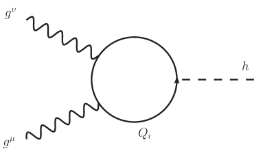
In the SM, the main contribution to the Higgs coupling to gluons comes from a top quark loop correction. In warped extra dimensional models there are many heavy KK quarks with important couplings with the Higgs, and thus one needs to add all of their contributions to the loop (see Figure 1), so that the resulting cross section for the process $gg\to h$ is

$$\sigma^{SM}_{gg\rightarrow h}={\alpha_{s}m_{h}^{2}\over 576\pi}\left|\sum_{Q}{y_{Q}\over m_{Q}}A_{1/2}(\tau_{Q})\right|^{2}\delta({\hat{s}}-m_{h}^{2}),$$ (21)

with $\tau_{Q}\equiv m^{2}_{h}/4m_{Q}^{2}$, $\hat{s}$ being the $gg$ invariant mass squared and $Q$ representing the physical fermions with physical Yukawa couplings $Y_{Q}$ and masses $m_{Q}$. The form factor is given by

$$A_{1/2}(\tau)={3\over 2}[\tau+(\tau-1)f(\tau)]\tau^{-2},$$ (22)

with

$$f(\tau)=\begin{cases}[\text{arcsin}\sqrt{\tau}]^{2}\qquad\;\qquad\;\qquad{\tau\leq 0}\\ -{1\over 4}\left[\text{ln}\left({1+\sqrt{1-\tau^{-1}}\over 1-\sqrt{1-\tau^{-1}}}\right)-i\pi\right]^{2}{\tau>1}.\end{cases}$$ (23)

The relevant quantity that we wish to evaluate is the effective coupling

$$c_{hgg}=\sum_{Q}{y_{Q}\over m_{Q}}A_{1/2}(\tau_{Q}),$$ (24)

where $y_{Q}$ is the $4D$ Yukawa coupling of fermion Q, in the mass eigenbasis, and $m_{Q}$ is its mass. In the gauge basis (the basis before spontaneous EW symmetry breaking) the Yukawa couplings are given by the following overlap integral along the fifth dimension,

$$Y_{Q_{i}U_{k}}^{u}=Y^{u}\int_{0}^{y_{1}}dye^{-4A(y)}h(y)Q_{L}^{u,(i)}(y)U_{R}^{(k)}(y),$$ (25)

and can be written as the following infinite dimensional Yukawa matrix, $\mathbf{Y}$

$$\begin{pmatrix}q_{L}^{0},\ Q_{L}^{i},\ U_{L}^{j}\end{pmatrix}\begin{pmatrix}Y^{u}_{{q}_{L}u_{R}}\ &0&Y^{u}_{{q}_{L}U_{R}^{b}}\ \\ Y^{u}_{{Q}_{L}^{i}u_{R}}\ &0&Y^{u}_{{Q}_{L}^{i}U_{R}^{b}}\ \\ 0&Y^{u*}_{{U}_{L}^{j}Q_{R}^{a}}\ &0\end{pmatrix}\begin{pmatrix}u_{R}^{0}\\ Q_{R}^{a}\\ U_{R}^{b}\end{pmatrix}.$$ (26)

In the same gauge basis we can also write down the infinite dimensional fermion mass matrix

$$\mathbf{M}=\begin{pmatrix}Y^{u}_{{q}_{L}u_{R}}\ v_{4}&0&Y^{u}_{{q}_{L}U_{R}^{b}}\ v_{4}\\ Y^{u}_{{Q}_{L}^{i}u_{R}}\ v_{4}&M_{Q}&Y^{u}_{{Q}_{L}^{i}U_{R}^{b}}\ v_{4}\\ 0&Y^{u*}_{{U}_{L}^{j}Q_{R}^{a}}\ v_{4}&M_{U}\end{pmatrix}.$$ (27)

where $v_{4}=174$ GeV is the Higgs vacuum expectation valued (VEV), and $M_{Q}$ and $M_{U}$ are the $n$-dimensional diagonal matrices of the tower of $n$ KK modes mass eigenvalues.

We proceed here by considering an effective field theory with only 3 KK levels, but we refer the reader to Section IV for a discussion involving the use of the full tower of KK fields. In our effective approach here, the previous matrices $\mathbf{M}$ and $\mathbf{Y}$ become $7\times 7$ truncated mass and Yukawa matrices. In order to use Eq. (24), we diagonalize numerically the mass matrix $\mathbf{M}$ above by a bi-unitary transformation. Performing the same transformation on the Yukawa matrix, $\mathbf{Y}$, one can finally use Eq. (24) to calculate the Higgs production cross section.

In all our numerical analysis we took $k=10^{18}$ GeV fixed, and then tuned all other parameters in such a way that all of the scenarios yield approximately the same zero mode masses (the SM quark masses) and the same lightest KK mode mass ($\simeq 2.1$ TeV). While this value for the lightest KK mass is already dangerously low for RS scenarios, in general warped models with modified $AdS_{5}$ metrics (like the CGQ and CPS scenarios considered here), such low KK masses can be safe from electroweak precision constraints as well as flavor constraints Cabrer ; Carmona:2011ib . The regime in which this happens is such that $kL_{1}\simeq 0.2$, and so we restrict ourselves to that region of parameter space when considering the modified models.

It is important to note that the zero mode masses are sensitive to the values of the Higgs localization parameter $a$ through Yukawa couplings

$$y={Y^{5D}\over\sqrt{k}}\int_{0}^{y_{1}}dye^{-4A(y)}h(y)q_{L}^{0}(y)u_{R}^{0}(y).$$ (28)

Using equations (6), (16) and (19) the above integral can be evaluated

$$y = -\frac{h_{0}}{f(c_{q})f(c_{u})}y_{s}((a-c_{q}+c_{u})(ky_{s}))^{\frac{c_{u}-c_{q}}{\nu^{2}}-1}e^{ky_{s}(a-c_{q}+c_{u})}\times$$

$$\left(\Gamma\left[(\frac{c_{q}-c_{u}}{\nu^{2}}+1),(a-c_{q}+c_{u})ky_{s}\right]-\Gamma\left[(\frac{c_{q}-c_{u}}{\nu^{2}}+1),(a-c_{q}+c_{u})k(y_{s}-y_{1})\right]\right).$$

In order to keep the 5D Yukawa couplings $Y^{5D}$ fixed for all of these models while requiring the correct SM quark masses, we have to set the values of $c_{q}$ and $c_{u}$ separately for each value of $a$, and for each different scenario. On a technical level, to be able to produce a correct top quark mass we had to set $Y^{5D}_{top}\simeq 3$ in all cases (so that even when we write $Y^{5D}\simeq 1$ in the left panel of Figure 2 we are still using $Y^{5D}_{top}\simeq 3$.).

To proceed further we need to include the flavor families of the SM, and to do so we will consider a simplified version of the SM model, that is, we take a $SM-like$ setup in which the 5D Yukawa couplings are diagonal, and thus we will ignore flavor inter-mixings in our loop calculation. With this simplifying assumption, it is straightforward to add the contributions of all the fermions running in the loop. This is of course not a viable scenario of flavor, but it does illustrate fairly the effects on Higgs production. Thus we consider the presence in the loop of five light quarks (which have negligible effect) and their associated KK quarks (which yield the main new contributions), as well as one SM top quark and its associated KK top quarks (the overall contribution from the top sector is actually very close to the SM top contribution). This simplified flavor structure for fermions is used in the three scenarios we consider, i.e. bulk-Higgs-RS, CGQ and CPS, and so we can obtain fair comparisons between the different predictions for Higgs production cross section generated by each model.

Figure 2: Higgs production rate ratio to Standard Model prediction as a function of the Higgs localization parameter, $a$. In all scenarios we consider an effective field theory consisting of a tower of 3 KK modes. The dashed line (blue) corresponds to the RS scenario with bulk Higgs. The solid and dotted lines correspond to the modified $Ads_{5}$ scenarios CGQ ($\nu=0.5$, $kL_{1}\simeq 0.27$) and CPS ($\nu=0.5$, $kL_{1}\simeq 0.29$) and the lightest KK mass is about $2.1$ TeV in all models. The 5D Yukawa coupling is varied between $Y^{5D}\sim 1$ (left panel), $Y^{5D}\sim 3$ (middle panel) and $Y^{5D}\sim 6$ (right panel). The shaded regions show the experimental bounds from CMS and ATLAS.

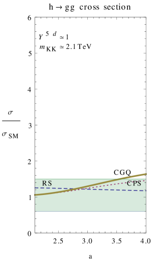
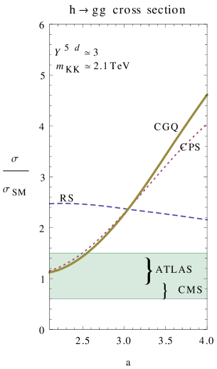
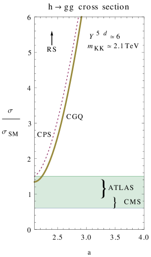
In the case of the CGQ scenario, the fermion bulk mass term is $M_{i}=c_{i}A^{\prime}(y)$ (see Eqs. (11) and (12)) and we used the values $\nu=0.5$, and $kL_{1}\equiv kL(y_{1})=0.27$ for the curvature radius as defined in equation (4). The $\delta=0.1$ criterion yields $a_{min}\simeq 2.09$ and the values for $c_{q}$ ($\simeq-c_{u}$) are being slightly decreased as $a$ becomes larger in order to keep the $Y^{5D}$ constant (as explained above). The CPS case is essentially the same model but with a constant fermionic bulk mass of $M_{i}=c_{i}k$ (see Eqs. (11) and 13)). We have again used the value $\nu=0.5$, but in order to keep the lightest KK mass fixed at the same value as the other models we set $kL_{1}\equiv kL(y_{1})=0.29$ for the curvature radius. The $\delta=0.1$ criterion this time yields $a_{min}\simeq 2.06$. Finally the RS scenario (with a bulk Higgs) is obtained in the limit $\nu>>1$ and $kL_{1}\rightarrow 1$. The numerical results obtained in this limit match the results obtained using the analytical RS formulae Azatov:2010pf ; Frank:2013un , providing thus a nontrivial consistency check of the procedure.

The results are shown in Figure 2, in which we plot the ratio of Higgs production cross section relative to the SM one, as a function of the Higgs localization parameter $a$ for the three models. The solid and dotted lines correspond to predictions from the CGQ and CPS models, respectively, while the dashed line represents the prediction of the RS scenario (with fermions and Higgs in the bulk). For each model, the numerical calculation involves the contributions from light quarks and 3 KK modes in the loop. The three panels correspond to different values for the 5D Yukawa coupling: $Y^{5D}\sim 1$ on the left side, $Y^{5D}\sim 3$ in the middle, and $Y^{5D}\sim 6$ on the right side. The shaded regions represent experimental restrictions on cross sections from CMS ($\mu\equiv{\sigma\over\sigma_{SM}}=0.8\pm 0.22$) and ATLAS ($\mu\equiv{\sigma\over\sigma_{SM}}=1.2\pm 0.3$) results Beringer:1900zz .

From all panels, it is clear that the behaviour of the CGQ and CPS models is very similar. In particular, both are very sensitive to the Higgs localization parameter $a$, while the RS model is much more stable against variations in $a$. Second, one can see that both modified warped models alleviate the enhancements in Higgs production present in RS models, but only for a small region of $a$, fortuitously the same region for which the electroweak constraints are satisfied Cabrer . The restriction becomes more stringent with increased $Y^{5D}$, so that for $Y^{5D}\sim 1$, the $a$ parameter can be anywhere between its minimal value $a_{min}$ and about $3-4$ (depending on the CGQ model or the CPS model), while for $Y^{5D}\sim 6$ the parameter $a$ is constrained to be in a really small region around $a_{min}$. By comparison, the RS model seems “safe” when $Y^{5D}\sim 1$, but then is completely disfavoured for $Y^{5D}\sim 3$ and $Y^{5D}\sim 6$ (where it lies outside the range of the figure).

The main message from these plots is that in the modified warped scenarios, the Higgs should be as de-localized as possible otherwise, if the Higgs is pushed towards the IR, the bounds become even worse than in RS (or at least the bounds we have considered here, namely those coming from LHC Higgs production). The reason for this behaviour with the parameter $a$ is that in the CGQ and CPS scenarios, the warp factor grows faster than in RS near the IR boundary. The effect of this is to actually concentrate the KK modes closer to the IR brane, and if one de-localizes sufficiently the Higgs profile away from the IR, the overlap integral between Higgs and KK fermions is suppressed with respect to the RS case. This leads to suppressed corrections to Higgs production, and we believe that this is also the origin for the suppressed contributions to electroweak and flavor observables.

Figure 3: Quark Yukawa couplings relative to their SM values, of a light quark (left panel) and the top quark (right panel) as a function of the Higgs localization parameter, $a$. In all scenarios we consider an effective field theory consisting of a tower of 3 KK levels with $Y^{5D}\sim 3$ and with the lightest KK mass at about $2.1$ TeV. The dashed line (blue) corresponds to RS with bulk Higgs. The solid and dotted lines correspond to the CGQ ($\nu=0.5$, $kL_{1}\simeq 0.27$) and CPS ($\nu=0.5$, $kL_{1}\simeq 0.29$) models of general metrics respectively.

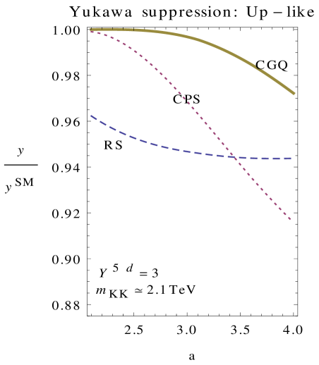
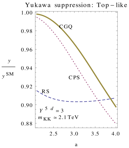
As a further check, in Figure 3 we plot the relative size of light quarks Yukawa couplings (left panel) and top quark Yukawa coupling (right panel) as a function of the Higgs localization parameter $a$, where both effects are computed by considering a truncated tower of just 3 KK fermion modes for each scenario. We choose $Y^{5D}\sim 3$ in all plots and here again we observe that the suppressed Yukawa couplings in the RS model are relatively independent of the Higgs de-localization, while in both the CPS and the CGQ scenarios, the suppression in these couplings depends dramatically on the localization parameter $a$. These effects confirm the findings of the previous figure, namely that for small $a$ (Higgs very de-localized) the modified warped scenarios produce very little effects in the Higgs sector, but these effects grow very quickly as the Higgs is pushed towards the TeV brane. The RS dependence on Higgs localization is much milder, but the effects are quantitatively quite large for the low KK masses considered here. We note here that even though the top Yukawa coupling can be quite suppressed, the scenarios still predict an enhancement in Higgs production. The reason is that the reduction produced by suppressed top couplings is balanced by the positive contribution due to the top KK tower. To this contribution, one must add the positive contributions of the other 5 towers of KK fermions (associated to the 5 other SM quarks) Azatov:2010pf .

Finally let us comment again that we have focused on a simplified version of the SM in which we ignored the flavor mixing between families, in order to simplify the sums in the loop calculation. Our main goal was to compare Higgs production among different models and study the general effects of the metric modification relative to the usual RS setup. A realistic scenario including the full flavor structure is underway, but the results should not be much different from the ones presented here, since flavor inter-mixings are not expected to produce big changes in the contributions to the loops generating the $hgg$ coupling.

IV Decoupling of the Heavy KK modes

In this section, we consider the effect of including the full tower of the KK modes on the evaluation of the Higgs production cross section, by performing the infinite sums analytically. Following the procedure given in Frank:2013un ; Azatov:2010pf we obtain the following expression for $c_{hgg}$, Eq. (24),

$$c_{hgg} = \text{Tr}(\mathbf{YM}^{-1})+\sum_{\rm light}{y_{Q}\over m_{Q}}(A_{1/2}(\tau_{Q})-1)$$ (29)

$$= -2{v_{4}}\sum_{i,j}{Y^{u}_{{Q_{L}}_{i}{U_{R}}_{j}}Y^{u*}_{{U_{L}}_{j}{Q_{R}}_{i}}\over M_{Q_{i}}M_{U_{j}}}+{y_{Q}\over m_{Q}}\big{|}_{\text{light}}A_{1/2}(\tau_{Q_{\rm light}}).$$ (30)

Here the couplings are the elements of the Yukawa matrix $\mathbf{Y}$ given in Eq. (26) and $\mathbf{M}$ is the fermion mass matrix in the gauge basis given by Eq. (27). We have also used the fact that $\mathbf{Y}={\partial\mathbf{M}\over\partial{v_{4}}}$ and therefore $\text{Tr}(\mathbf{YM}^{-1})=\text{Tr}({\partial\mathbf{M}\over\partial{v_{4}}}\mathbf{M}^{-1})={\partial\text{ln Det}(\mathbf{M})\over\partial v_{4}}$.

Since the form factor, $A_{1/2}$ is negligible for the light fermion generations, we can neglect the last term in Eq. (29), and using Eq. (25) we have

$$c_{hgg}=-2{v_{4}}Y^{u}Y^{u*}\sum_{i,j}\int dydy^{\prime}e^{-4A(y)}e^{-4A(y^{\prime})}{Q^{(i)}_{L}(y)Q^{(i)}_{R}(y^{\prime})\over M_{Q_{i}}}{U^{(j)}_{R}(y)U^{(j)}_{L}(y^{\prime})\over M_{U_{j}}}h(y)h(y^{\prime}),\ \ \ \$$ (31)

where the Higgs profile is given in Eq. (6). The infinite sums in this equation can be performed using the completeness of the Sturm-Liouville system. We have (see the Appendix)

$$\sum_{n=1}^{\infty}{{\hat{U}}_{R}^{(n)}(y){\hat{U}}_{L}^{(n)}(y^{\prime})\over m_{n}}=e^{Q(y)-Q(y^{\prime})}\left[\theta(y^{\prime}-y)-{\int_{0}^{y^{\prime}}e^{A-2Q}\over\int_{0}^{y_{1}}e^{A-2Q}}\right]$$ (32)

$$\sum_{n=1}^{\infty}{{\hat{Q}}_{L}^{(n)}(y){\hat{Q}}_{R}^{(n)}(y^{\prime})\over m_{n}}=-e^{Q(y^{\prime})-Q(y)}\left[\theta(y^{\prime}-y)-{\int_{0}^{y^{\prime}}e^{A+2Q}\over\int_{0}^{y_{1}}e^{A+2Q}}\right].$$ (33)

Inserting this back into Eq. (31) for $c_{hgg}$ we can finally calculate the $hgg$ cross section.

Figure 4: Higgs production rate via gluon fusion in the CGQ scenario. The solid thick line (blue) shows the contribution due to the full tower of KK modes. The dashed (red), dotted (khaki) and thin solid (green) lines show the contribution due to a tower of 3, 2 and 1 KK modes respectively. The shaded region shows the experimental bounds from CMS and ATLAS.

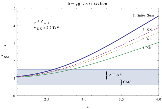
Figure 4 shows the result of evaluating the Higgs production cross section using the infinite KK tower, compared to the result obtained using effective field theories with one, two and three KK modes. As we can see, the result obtained using a very small number of modes converge quickly to the result using infinite sum, which means that the heavy KK modes decouple from the evaluation of the cross section. The decoupling of heavy modes is particularly true in the region where the Higgs production cross section is safe from large enhancements from the presence of KK modes in the loop. This observation seems to imply that at least for the observable considered here, the Higgs production rate, the 5D warped models with bulk Higgs, which are essentially valid only up to $\Lambda_{UV}\sim\cal{O}(\text{10 TeV})$, are calculable and the effects of higher order operators should be suppressed (see also Frank:2013un ).

V Conclusions

In this work we calculated the Higgs production rate via gluon fusion in 5D scenarios with modified $AdS_{5}$ metrics. In the SM, the Higgs production cross section is determined by the coupling of the top quark to the Higgs field. Just like in RS, the deviations from the SM in modified $AdS_{5}$ models are caused by the presence of extra KK fermion towers, associated to each of the six SM quarks, and their couplings to the Higgs field. These KK fermions circulate through the loop responsible for the Higgs production through gluon fusion, and they can lead to large enhancements in the Higgs production cross section. In RS models with fermions and Higgs fields propagating in the bulk, depending on the values of the 5D Yukawa couplings, the enhancements can reach 50% if the lightest KK mass is $\sim 2$ GeV (at odds with ATLAS and CMS data). In fact the new data from LHC Higgs searches have become a stringent bound on warped scenarios, to be considered together with flavor and electroweak precision tests.

The couplings with the KK fields are generated by the overlap of the KK fermions wavefunctions and the Higgs profiles along the fifth dimension, thus the localization of these fields is crucial to the calculation. In the general warped scenarios, the KK fermions are pushed towards the IR brane compared to the RS model due to the metric growth near that boundary. On the other hand the localization of the Higgs profile along the 5th dimension is controlled by a free parameter $a$: the smaller the values for $a$, the less localized the Higgs profile. Our results show that a more de-localized Higgs field leads to a more SM-like Higgs production, due to suppressed overlap integrals between Higgs and KK fermions. Moreover, this seems to happen in the parameter region which is also safe from electroweak and flavor precision tests. We have also shown, by comparing the results obtained using a small number of modes with the effects of the whole KK tower, that the former converges quickly to the latter in the same region, leading further support to the validity of our calculation.

Thus we have shown that, based on results from Higgs production, the modified $AdS_{5}$ scenarios considered here are consistent with the experimental results for light KK masses of $\sim 2$ TeV (unlike RS models). This was a non-trivial check, and necessary, since while these scenarios had proved to be safer in terms of precision tests (electroweak and flavor) compared to RS, the new Higgs production data from the LHC might have been in conflict with the effects from the models. Our results confirm the viability of these scenarios, which allow for new physics at lower scales than conventional RS models and thus could yield signals at the LHC in the near future.

VI Acknowledgements

We thank NSERC for partial financial support under grant number SAP105354.

VII Appendix

In this appendix we show how to obtain the infinite sums in Eq. (31). Using the equations of motion for the fermion field profiles before the electroweak symmetry breaking, from the $S_{matter}$ one gets

$$\partial_{y}{\hat{\psi}}_{L}+M_{\psi}(y){\hat{\psi}}_{L}=e^{A(y)}m_{n}{\hat{\psi}}_{R},$$

$$-\partial_{y}{\hat{\psi}}_{R}+M_{\psi}(y){\hat{\psi}}_{R}=e^{A(y)}m_{n}{\hat{\psi}}_{L},$$

and using the definition (11) we obtain

$$m_{n}{\hat{\psi}}_{R}-e^{-A-Q}\partial_{y}({\hat{\psi}}_{L}e^{Q})=0,$$ (34)

$$m_{n}{\hat{\psi}}_{L}+e^{-A+Q}\partial_{y}({\hat{\psi}}_{R}e^{-Q})=0,$$ (35)

where the hatted functions are defined as ${\hat{\psi}}\equiv e^{-2A}\psi$. We now multiply the first equation by $e^{A+Q}$ and the second by $e^{A-Q}$. Integrating from $0$ to some arbitrary value, $y^{\prime}$, gives,

$$\int_{0}^{y^{\prime}}e^{A+Q}{\hat{\psi}}_{R}={1\over m_{n}}{\hat{\psi}}_{L}(y^{\prime})e^{Q(y^{\prime})},$$ (36)

$$\int_{0}^{y^{\prime}}e^{A-Q}{\hat{\psi}}_{L}=-{1\over m_{n}}{\hat{\psi}}_{R}(y^{\prime})e^{-Q(y^{\prime})},$$ (37)

where we have imposed Dirichlet boundary conditions, ${\hat{\psi}}_{L}(0)=0$ on the first equation, and ${\hat{\psi}}_{R}(0)=0$ on the second one. Multiplying these equations by ${\hat{\psi}}_{R}(y^{\prime\prime})$ and ${\hat{\psi}}_{L}(y^{\prime\prime})$ and performing a summation over all of the KK modes we obtain

$$\int_{0}^{y^{\prime}}e^{A+Q}\sum_{n=1}^{\infty}{\hat{\psi}}_{R}^{(n)}(y^{\prime\prime}){\hat{\psi}}_{R}^{(n)}(y)=e^{Q(y^{\prime})}\sum_{n=1}^{\infty}{{\hat{\psi}}_{R}^{(n)}(y^{\prime\prime}){\hat{\psi}}_{L}^{(n)}(y^{\prime})\over m_{n}},$$ (38)

$$\int_{0}^{y^{\prime}}e^{A-Q}\sum_{n=1}^{\infty}{\hat{\psi}}_{L}^{(n)}(y^{\prime\prime}){\hat{\psi}}_{L}^{(n)}(y)=-e^{-Q(y^{\prime})}\sum_{n=1}^{\infty}{{\hat{\psi}}_{L}^{(n)}(y^{\prime\prime}){\hat{\psi}}_{R}^{(n)}(y^{\prime})\over m_{n}}.$$ (39)

Now using the completeness of the Sturm-Liouville system as

$$\sum_{n=0}^{\infty}{\hat{\psi}}^{(n)}(y){\hat{\psi}}^{(n)}(y^{\prime})=e^{-A}\delta(y-y^{\prime}),$$ (40)

we obtain the sums

$$\sum_{n=1}^{\infty}{{\hat{\psi}}_{R}^{(n)}(y^{\prime\prime}){\hat{\psi}}_{L}^{(n)}(y^{\prime})\over m_{n}}=e^{-Q(y^{\prime})}\int_{0}^{y^{\prime}}e^{A+Q}\left[e^{-A}\delta(y^{\prime\prime}-y)-{\hat{\psi}}^{(0)}_{R}(y^{\prime\prime}){\hat{\psi}}^{(0)}_{R}(y)\right],$$ (41)

$$\sum_{n=1}^{\infty}{{\hat{\psi}}_{L}^{(n)}(y^{\prime\prime}){\hat{\psi}}_{R}^{(n)}(y^{\prime})\over m_{n}}=-e^{Q(y^{\prime})}\int_{0}^{y^{\prime}}e^{A-Q}\left[e^{-A}\delta(y^{\prime\prime}-y)-{\hat{\psi}}^{(0)}_{L}(y^{\prime\prime}){\hat{\psi}}^{(0)}_{L}(y)\right].$$ (42)

Finally performing the $\delta$-function integrals and using the normalized zero modes ($y_{1}$ being the position of the IR brane)

$${\hat{\psi}}_{L}^{(0)}(y)={e^{-Q(y)}\over(\int_{0}^{y_{1}}e^{A-2Q})^{1\over 2}},\ {\hat{\psi}}_{R}^{(0)}(y)={e^{Q(y)}\over(\int_{0}^{y_{1}}e^{A+2Q})^{1\over 2}},$$ (43)

we get

$$\sum_{n=1}^{\infty}{{\hat{\psi}}_{R}^{(n)}(y^{\prime\prime}){\hat{\psi}}_{L}^{(n)}(y^{\prime})\over m_{n}}=e^{Q(y^{\prime\prime})-Q(y^{\prime})}\left[\theta(y^{\prime}-y^{\prime\prime})-{\int_{0}^{y^{\prime}}e^{A-2Q}\over\int_{0}^{y_{1}}e^{A-2Q}}\right],$$ (44)

$$\sum_{n=1}^{\infty}{{\hat{\psi}}_{L}^{(n)}(y^{\prime\prime}){\hat{\psi}}_{R}^{(n)}(y^{\prime})\over m_{n}}=-e^{Q(y^{\prime})-Q(y^{\prime\prime})}\left[\theta(y^{\prime}-y^{\prime\prime})-{\int_{0}^{y^{\prime}}e^{A+2Q}\over\int_{0}^{y_{1}}e^{A+2Q}}\right].$$ (45)

References

- (1) L. Randall and R. Sundrum, Phys. Rev. Lett. 83, 3370 (1999); L. Randall and R. Sundrum, Phys. Rev. Lett. 83, 4690 (1999).
- (2) H. Davoudiasl, J. L. Hewett and T. G. Rizzo, Phys. Lett. B 473, 43 (2000).
- (3) A. Pomarol, Phys. Lett. B 486, 153 (2000).
- (4) Y. Grossman and M. Neubert, Phys. Lett. B 474, 361 (2000).
- (5) S. Chang, J. Hisano, H. Nakano, N. Okada and M. Yamaguchi, Phys. Rev. D 62, 084025 (2000).
- (6) T. Gherghetta and A. Pomarol, Nucl. Phys. B 586, 141 (2000).
- (7) H. Davoudiasl, J. L. Hewett and T. G. Rizzo, Phys. Rev. D 63, 075004 (2001).
- (8) M. S. Carena, A. Delgado, E. Ponton, T. M. P. Tait and C. E. M. Wagner, Phys. Rev. D 71, 015010 (2005); M. S. Carena, A. Delgado, E. Ponton, T. M. P. Tait and C. E. M. Wagner, Phys. Rev. D 68, 035010 (2003); A. Delgado and A. Falkowski, JHEP 0705, 097 (2007).
- (9) C. Csaki, C. Delaunay, C. Grojean and Y. Grossman, JHEP 0810, 055 (2008).
- (10) K. Agashe, R. Contino, L. Da Rold and A. Pomarol, Phys. Lett. B 641, 62 (2006).
- (11) S. J. Huber, Nucl. Phys. B 666, 269 (2003).
- (12) K. Agashe, A. Delgado, M. J. May and R. Sundrum, JHEP 0308 (2003) 050.
- (13) C. Csaki, A. Falkowski and A. Weiler, JHEP 0809, 008 (2008) [arXiv:0804.1954 [hep-ph]].
- (14) J. Santiago, JHEP 0812, 046 (2008).
- (15) C. Csaki, A. Falkowski and A. Weiler, Phys. Rev. D 80, 016001 (2009).
- (16) K. Agashe, A. Azatov and L. Zhu, Phys. Rev. D 79, 056006 (2009) [arXiv:0810.1016 [hep-ph]].
- (17) J. A. Cabrer, G. von Gersdorff and M. Quiros, New J. Phys. 12, 075012 (2010); J. A. Cabrer, G. von Gersdorff and M. Quiros, Phys. Lett. B 697, 208 (2011); J. A. Cabrer, G. von Gersdorff and M. Quiros, JHEP 1105, 083 (2011); J. A. Cabrer, G. von Gersdorff and M. Quiros, Phys. Rev. D 84, 035024 (2011); J. A. Cabrer, G. von Gersdorff and M. Quiros, JHEP 1201, 033 (2012).
- (18) A. Carmona, E. Ponton and J. Santiago, JHEP 1110, 137 (2011).
- (19) S. Mert Aybat and J. Santiago, Phys. Rev. D 80, 035005 (2009); A. Delgado and D. Diego, Phys. Rev. D 80, 024030 (2009).
- (20) J. de Blas, A. Delgado, B. Ostdiek and A. de la Puente, Phys. Rev. D 86, 015028 (2012).
- (21) A. Azatov, M. Toharia and L. Zhu, Phys. Rev. D 82, 056004 (2010).
- (22) S. Casagrande, F. Goertz, U. Haisch, M. Neubert and T. Pfoh, JHEP 1009, 014 (2010).
- (23) M. Frank, N. Pourtolami and M. Toharia, Phys. Rev. D 87, 096003 (2013).
- (24) K. Agashe: private communication (2012)
- (25) A. Azatov, M. Toharia and L. Zhu, Phys. Rev. D 80, 035016 (2009).
- (26) K. Agashe and R. Contino, Phys. Rev. D 80, 075016 (2009).
- (27) W. D. Goldberger and M. B. Wise, Phys. Rev. Lett. 83, 4922 (1999); W. D. Goldberger and M. B. Wise, Phys. Lett. B 475, 275 (2000).
- (28) S. S. Gubser, Adv. Theor. Math. Phys. 4, 679 (2000).
- (29) J. Beringer et al. [Particle Data Group Collaboration], Phys. Rev. D 86, 010001 (2012) (url: http://pdg.lbl.gov).