institutetext: a Institute for Theoretical Physics and Spinoza Institute,
   Utrecht University, 3508 TD Utrecht, The Netherlands.
b Dipartimento di Fisica, Università di Milano-Bicocca,
   Piazza della Scienza 3, 20126 Milano, Italy, and
   INFN, sezione di Milano–Bicocca, Piazza della Scienza 3, 20126 Milano, Italy.
c Dipartimento di Fisica, Università di Milano,
   Via Celoria 16, 20133 Milano, Italy, and
   INFN, sezione di Milano, Via Celoria 16, 20133 Milano, Italy.
d Department of Mathematics and Center for Mathematical Physics,
   University of Hamburg, Bundesstrasse 55, 20146 Hamburg, Germany.

Rotating black holes in 4d gauged supergravity

Alessandra Gnecchia, Kiril Hristovb, Dietmar Klemmc, Chiara Toldoa and Owen Vaughand
Abstract

We present new results towards the construction of the most general black hole solutions in four-dimensional Fayet-Iliopoulos gauged supergravities. In these theories black holes can be asymptotically AdS and have arbitrary mass, angular momentum, electric and magnetic charges and NUT charge. Furthermore, a wide range of horizon topologies is allowed (compact and noncompact) and the complex scalar fields have a nontrivial radial and angular profile. We construct a large class of solutions in the simplest single scalar model with prepotential $F=-iX^{0}X^{1}$ and discuss their thermodynamics. Moreover, various approaches and calculational tools for facing this problem with more general prepotentials are presented.

Keywords:
Black Holes in String Theory, AdS-CFT Correspondence, Superstring Vacua
preprint: ITP-UU-13/28
SPIN-13/19
IFUM-1018-FT
ZMP-HH/13-21

1 Introduction

The construction and physical understanding of 4d black hole solutions in supersymmetric theories with negative cosmological constant is relevant for a number of developments in high energy physics. One can try to analyze such solutions in their own right as string theory ground states and understand black hole thermodynamics Bekenstein:1973ur ; Hawking:1974sw ; Hawking:1982dh ; Hawking:1998kw ; Chamblin:1999tk ; Cvetic:1999ne ; Chamblin:1999hg ; Caldarelli:1999xj ; Hristov:2013sya and microscopic degeneracy Strominger:1996sh ; Maldacena:1997de ; Dijkgraaf:1996it ; Strominger:1997eq , guided by the AdS/CFT correspondence. In this sense black holes are the best test ground for the fundamental principles of quantum gravity, and therefore the knowledge of all possible black hole solutions in a given theory can be regarded as a first step in the programme of solving this theory on a quantum level. Alternatively, these gravitational systems provide non-trivial asymptotically AdS backgrounds with holographic duals that exhibit a rich structure and a wide range of applications in field theory and condensed matter systems, see e.g. Hartnoll:2009sz ; Herzog:2009xv ; McGreevy:2009xe ; Sachdev:2010ch ; Barisch:2011ui ; Anninos:2013mfa .

In the present paper we address the question of how to find generic AdS black hole solutions in theories with $\text{U}(1)$ gauge fields and scalars that arise in the framework of gauged supergravity. Such solutions will be labeled by a set of conserved charges, corresponding to the global symmetries of the system - in four dimensions these are the mass, NUT charge, angular momentum, electric and magnetic charges of the $\text{U}(1)$ gauge fields, and possible scalar hair. Unlike asymptotically flat black holes which only have spherical horizons, solutions in AdS can be further distinguished by their horizon topology Vanzo:1997gw . In the compact case the horizons can be Riemann surfaces of arbitrary genus, while noncompact horizons correspond for example to black brane solutions.

There have been numerous partial results on the topic in the last decade. Due to the lack of electromagnetic duality in the electrically gauged theories that are usually considered111Note that restoring the duality only rotates electric and magnetic charges, without changing the types of black hole classes, thus the discussion remains true, upto redefinition of the meaning of electric and magnetic charges., the various classes of solutions that were found look considerably different depending on the types of charges switched on. The known classes of electric solutions include both extremal and thermal, static and rotating solutions Duff:1999gh ; Chong:2004na ; Chow:2010sf ; Chow:2010fw , where in the BPS limit the known solutions are necessarily rotating Caldarelli:1998hg ; AlonsoAlberca:2000cs with constant scalars. The available magnetic black holes222Dyonic AdS black holes were constructed recently in Lu:2013ura . can instead be BPS only in the static limit Cacciatori:2009iz (with the exception of one hyperbolic rotating solution Klemm:2011xw ) with nonconstant scalars, see also Dall'Agata:2010gj ; Hristov:2010ri 333See Halmagyi:2013sla ; Halmagyi:2013qoa for black hole solutions of this type in theories with nontrivial hypermultiplets.. Their non-BPS and thermal generalizations were also known only with vanishing angular momentum Klemm:2012yg ; Toldo:2012ec ; Klemm:2012vm ; Gnecchi:2012kb . We show that all these seemingly disjoint classes in fact fall inside a single general solution, once we allow not only for rotation and electric and magnetic charges, but also for NUT charge. This extra freedom allows us to find a large parameter space of black hole solutions in one of the possible models (with prepotential $F=-iX^{0}X^{1}$) and gives strong hints on how to tackle the same problem with more complicated scalar manifolds.

We also discuss an alternative but complementary approach to constructing solutions which is based on dimensional reduction and the real formulation of special geometry, as developed in Mohaupt:2011aa . Within this formalism, the problem of constructing stationary solutions of $4D,\,{\cal N}=2$ Fayet-Iliopoulos gauged supergravity reduces to solving a particular three-dimensional Euclidean non-linear sigma model (with potential). Previously this appraoch has been used to construct static black hole solutions Klemm:2012yg ; Klemm:2012vm , whereas in this paper we are interested in rotating solutions and the procedure is adapted accordingly. As an application, we present the new rotating black hole solutions of the $F=-iX^{0}X^{1}$ model within this formalism, thus providing a useful consistency check.

The plan of the paper is as follows. We briefly present the Lagrangian and equations of motion of the theory at the end of this section. Section 2 contains a general discussion of the universal structure of black holes based on the Carter-Plebański metric Carter:1968ks ; Plebanski:1975 , relating it to various examples existing in the literature. In the same section we comment on the difference between over- and under-rotating extremal solutions in AdS, and we explain how to choose different horizon topologies. In section 3 we study the theory with prepotential $F=-iX^{0}X^{1}$ and find a general class of nonextremal black holes with angular momentum and magnetic charges. We discuss the thermodynamics and physical properties of these solutions, showing a new type of limit leading to noncompact horizons with finite area. In section 4, these solutions are extended to allow for NUT- and electric charges, however the NUT charge will not be allowed to take arbitrary values. We also show how the solutions can be written in terms of harmonic functions and special geometry quantities and how in the limit of vanishing gauging a class of known solutions to ungauged supergravity LozanoTellechea:1999my is recovered. We end the main discussion of the paper with some general comments and suggestions in section 5. Some of the useful tools and techniques we used to obtain our main results are relegated to the appendices. In app. A we consider supersymmetric rotating attractors, showing that all asymptotically flat under-rotating attractors are precisely half-BPS (in Hristov:2012nu they were shown to be at least quarter-BPS). In app. B we give more details about the real formulation of special geometry.

Note added: During the write-up of our work, ref. Chow:2013gba appeared, where charged rotating solutions of the same model were presented.

1.1 Lagrangian and equations of motion

A detailed description of notations and conventions of abelian $\mathcal{N}=2$ gauged supergravity can be found in Andrianopoli:1996cm . In the context of black hole physics, such models are also discussed in Cacciatori:2009iz ; Klemm:2010mc ; Dall'Agata:2010gj ; Hristov:2010ri , and we refer the reader to those papers for a complete introduction.

The most general bosonic Lagrangian of ${\cal N}=2$ abelian Fayet-Iliopoulos (FI) gauged supergravity is given by444We use the convention $F_{\mu\nu}=\frac{1}{2}(\partial_{\mu}A_{\nu}-\partial_{\nu}A_{\mu})$ for the field strengths. Our signature is mostly plus, and $\epsilon_{0123}=-\epsilon^{0123}=1$.

$$e^{-1}{\cal L}=\frac{1}{2}R-g_{i\bar{\jmath}}\partial^{\mu}z^{i}\partial_{\mu}\bar{z}^{\bar{\jmath}}+I_{\Lambda\Sigma}(z,\bar{z})F_{\mu\nu}^{\Lambda}F^{\mu\nu|\Sigma}+\frac{1}{2}R_{\Lambda\Sigma}(z,\bar{z})\epsilon^{\mu\nu\rho\sigma}F_{\mu\nu}^{\Lambda}F_{\rho\sigma}^{\Sigma}-g^{2}V(z,\bar{z})\,,$$ (1)

with $\Lambda,\Sigma=0,1...,n_{V}$ and $i,j=1,...,n_{V}$, where $n_{V}$ is the number of vector multiplets. The imaginary and the real part of the period matrix $\mathcal{N}_{\Lambda\Sigma}$ ($I_{\Lambda\Sigma}$ and $R_{\Lambda\Sigma}$), as well as the metric on the scalar moduli space $g_{i\bar{\jmath}}$ and the scalar potential $V$, depend on the particular vector multiplet model. The complex scalars $z^{i}$ are written in terms of the holomorphic symplectic sections $(X^{\Lambda},F_{\Lambda})$. All these quantities can be specified uniquely just with a single holomorphic function, $F(X)$, the prepotential. Therefore specifying the prepotential is equivalent to defining the full Lagrangian.

The Einstein equations following from (1) read

$$-(R_{\mu\nu}-\frac{1}{2}g_{\mu\nu}R)=g_{\mu\nu}g^{2}V(z,\bar{z})+g_{\mu\nu}\partial^{\sigma}z^{i}\partial_{\sigma}\bar{z}^{\bar{\jmath}}g_{i\bar{\jmath}}-2g_{i\bar{\jmath}}\partial_{(\mu}z^{i}\partial_{\nu)}\bar{z}^{\bar{\jmath}}+$$
$$-I_{\Lambda\Sigma}g_{\mu\nu}F_{\rho\sigma}^{\Lambda}F^{\rho\sigma|\Sigma}+4I_{\Lambda\Sigma}F_{\mu\alpha}^{\Lambda}{F_{\nu}}^{\alpha|\Sigma}\,,$$ (2)

while the equations of motion for the scalar fields $z^{i}$ are given by

$$g_{i\bar{\jmath}}\partial_{\mu}(e\partial^{\mu}\bar{z}^{\bar{\jmath}})+e\frac{\partial g_{i\bar{k}}}{\partial\bar{z}^{\bar{\jmath}}}\partial^{\mu}\bar{z}^{\bar{\jmath}}\partial_{\mu}\bar{z}^{\bar{k}}+e\frac{\partial I_{\Lambda\Sigma}}{\partial z^{i}}F_{\rho\sigma}^{\Lambda}F^{\rho\sigma|\Sigma}+\frac{e}{2}\frac{\partial R_{\Lambda\Sigma}}{\partial z^{i}}\epsilon^{\mu\nu\rho\sigma}F_{\mu\nu}^{\Lambda}F_{\rho\sigma}^{\Sigma}-eg^{2}\frac{\partial V}{\partial z^{i}}=0\,,$$ (3)

and the Maxwell equations for the vector fields $A_{\nu}^{\Lambda}$ are

$$\partial_{\mu}(eF^{\mu\nu\,|\Sigma}I_{\Sigma\Lambda}+\frac{e}{2}\epsilon^{\mu\nu\rho\sigma}F_{\rho\sigma}^{\Sigma}R_{\Lambda\Sigma})=0\,.$$ (4)

The requirement of an asymptotic $\text{AdS}_{4}$ geometry fixes the values of the scalar fields at infinity. Indeed, $\text{AdS}_{4}$ corresponds to an extremum of the scalar potential, yielding the asymptotic attractor condition

$\displaystyle\left.\frac{\partial V}{\partial z^{i}}\right|_{\infty}=0\ ,\qquad\Leftrightarrow\qquad\xi_{\Lambda}D_{i}X^{\Lambda}\big{|}_{\infty}=0\ ,$ (5)

where $D_{i}X^{\Lambda}$ is the Kähler covariant derivative of the coordinates $X^{\Lambda}$ with respect to $z^{i}$. The constants $\xi_{\Lambda}$ determine which linear combination $\xi_{\Lambda}A^{\Lambda}$ is used to gauge a $\text{U}(1)$ subgroup of the $\text{SU}(2)$ R-symmetry. In what follows, we shall use $g_{\Lambda}\equiv g\xi_{\Lambda}$, with $g$ the gauge coupling constant appearing in (1).

2 Universal structure of rotating black holes

This section is devoted to showing that all known rotating black holes in matter-coupled ${\cal N}=2$ gauged supergravity in four dimensions have a universal metric structure. It turns out that in all cases the metric can be cast in the form

$$ds^{2}=-f(dt+\omega_{y}dy)^{2}+f^{-1}\left[v\left(\frac{dq^{2}}{Q}+\frac{dp^{2}}{P}\right)+PQdy^{2}\right]\,,$$ (6)

where $Q(q)$ and $P(p)$ are polynomials of fourth degree respectively in the variables $q$ (radial variable) and $p$ (function of the angular variable $\theta$). The warp factors $f$, $v$, $\omega_{y}$ are more general functions of $q$ and $p$. We start now with the examples and finish the section by commenting on some novel general features of this metric, such as the difference between over- and under-rotating solutions and the relation between the function $P(p)$ and the choice of horizon topology.

2.1 Carter-Plebański solution

The metric and $\text{U}(1)$ field strength of the Carter-Plebański solution Carter:1968ks ; Plebanski:1975 of minimal gauged supergravity are respectively given by

$$ds^{2}=-\frac{Q(q)}{p^{2}+q^{2}}(d\tau-p^{2}d\sigma)^{2}+\frac{p^{2}+q^{2}}{Q(q)}dq^{2}+\frac{p^{2}+q^{2}}{P(p)}dp^{2}+\frac{P(p)}{p^{2}+q^{2}}(d\tau+q^{2}d\sigma)^{2}\,,$$ (7)
$$F=\frac{\mathsf{Q}(p^{2}-q^{2})+2\mathsf{P}pq}{(p^{2}+q^{2})^{2}}{\rm d}q\wedge({\rm d}\tau-p^{2}{\rm d}\sigma)+\frac{\mathsf{P}(p^{2}-q^{2})-2\mathsf{Q}pq}{(p^{2}+q^{2})^{2}}{\rm d}p\wedge({\rm d}\tau+q^{2}{\rm d}\sigma)\,,$$ (8)

where the quartic structure functions read

$\displaystyle P(p)$ $\displaystyle=$ $\displaystyle\alpha-\mathsf{P}^{2}+2np-\varepsilon p^{2}+(-\Lambda/3)p^{4}\,,$
$\displaystyle Q(q)$ $\displaystyle=$ $\displaystyle\alpha+\mathsf{Q}^{2}-2mq+\varepsilon q^{2}+(-\Lambda/3)q^{4}\,.$ (9)

Here, $\mathsf{Q}$, $\mathsf{P}$ and $n$ denote the electric, magnetic and NUT-charge respectively, $m$ is the mass parameter, while $\alpha$ and $\varepsilon$ are additional non-dynamical constants.

By making the coordinate transformation

$$\tau=At+By\,,\qquad\sigma=Ct+Dy\,,\qquad AD-BC=1\,,$$ (10)

(7) can be cast into the form (6), where

$$v=Q(A-p^{2}C)^{2}-P(A+q^{2}C)^{2}\,,\qquad f=\frac{v}{p^{2}+q^{2}}\,,$$ (11)

and

$$\omega_{y}=\frac{1}{v}\left[Q(A-p^{2}C)(B-p^{2}D)-P(A+q^{2}C)(B+q^{2}D)\right]\,.$$ (12)

We see that there is actually more than one way to write (7) as a fibration (6) over a three-dimensional base space. A simple choice would be for instance $A=D=1$, $B=C=0$, such that

$$v=Q-P\,,\qquad\omega_{y}=\frac{Qp^{2}+Pq^{2}}{P-Q}\,.$$

2.2 Rotating magnetic BPS black holes, prepotential $F=-iX^{0}X^{1}$

Our second example is the family of BPS magnetic rotating black holes in the model with prepotential $F=-iX^{0}X^{1}$, constructed in Klemm:2011xw .

This model has just one complex scalar $\tau$. The symplectic sections in special coordinates are $v^{T}=\left(1,\tau,-i\tau,-i\right)$. The Kähler potential, metric and vector kinetic matrix are respectively of this form:

$$e^{-{\cal K}}=2(\tau+\bar{\tau})\ ,\qquad g_{\tau\bar{\tau}}=\partial_{\tau}\partial_{\bar{\tau}}{\cal K}=(\tau+\bar{\tau})^{-2}\ ,$$ (13)
$${\cal N}=\left(\begin{array}[]{cc}-i\tau&0\\ 0&-\frac{i}{\tau}\end{array}\right)\ ,$$ (14)

thus requiring ${\mathrm{Re}}\tau>0$. For our choice of electric gauging, the scalar potential is

$$V=-\frac{4}{\tau+\bar{\tau}}(g_{0}^{2}+2g_{0}g_{1}\tau+2g_{0}g_{1}\bar{\tau}+g_{1}^{2}\tau\bar{\tau})\ ,$$ (15)

which has an extremum at $\tau=\bar{\tau}=|g_{0}/g_{1}|$.

The metric of the BPS solution of Klemm:2011xw reads

$\displaystyle ds^{2}=$ $\displaystyle\frac{p^{2}+q^{2}-\Delta^{2}}{P}dp^{2}+\frac{P}{p^{2}+q^{2}-\Delta^{2}}\left(dt+(q^{2}-\Delta^{2})dy\right)^{2}$ (16)
$\displaystyle+\frac{p^{2}+q^{2}-\Delta^{2}}{Q}dq^{2}-\frac{Q}{p^{2}+q^{2}-\Delta^{2}}\left(dt-p^{2}dy\right)^{2}\ ,$

with the structure functions

$$P=(1+A)\frac{\mathsf{E}^{2}l^{2}}{4}-\mathsf{E}p^{2}+\frac{p^{4}}{l^{2}}\ ,\qquad Q=\frac{1}{l^{2}}\left(q^{2}+\frac{\mathsf{E}l^{2}}{2}-\Delta^{2}\right)^{2}\ .$$ (17)

The upper parts of the (nonholomorphic) symplectic section $(L^{\Lambda},M_{\Lambda})$ and the $\text{U}(1)$ gauge potentials are given by

$$L^{0}=\frac{1}{2}\!\left(\frac{g_{1}}{g_{0}}\right)^{\frac{1}{2}}\!\!\left(\frac{p^{2}+(q-\Delta)^{2}}{p^{2}+q^{2}-\Delta^{2}}\right)^{\frac{1}{2}}\,,\quad L^{1}=\frac{1}{2}\!\left(\frac{g_{0}}{g_{1}}\right)^{\frac{1}{2}}\!\!\frac{p^{2}+q^{2}-\Delta^{2}+2ip\Delta}{\left[(p^{2}+q^{2}-\Delta^{2})(p^{2}+(q-\Delta)^{2})\right]^{\frac{1}{2}}}\,,$$
$$A^{\Lambda}=-\frac{\mathsf{E}p\sqrt{-A}}{4g_{\Lambda}(p^{2}+q^{2}-\Delta^{2})}(dt+(q^{2}-\Delta^{2})dy)\,,\qquad\Lambda=0,1\,.$$

The solution is thus specified by three free parameters $A,\mathsf{E},\Delta$. (The asymptotic AdS curvature radius $l$ is related to the gauge coupling constants by $l^{-2}=4g_{0}g_{1}$). The new rotating solution that we are going to describe in section 3 is a nonextremal deformation of this solution. For $\Delta=0$, the moduli are constant, and the solution reduces to a subclass of (7), (8).

The metric (16) can again be written in the form (6), where now

$$v=Q-P\,,\qquad f=\frac{v}{p^{2}+q^{2}-\Delta^{2}}\,,$$ (18)
$$\omega_{y}=\frac{P(q^{2}-\Delta^{2})+Qp^{2}}{P-Q}\,.$$ (19)

2.3 Rotating black holes of Chong, Cvetič, Lu, Pope and Chow

Finally, there are three other examples of rotating black hole solutions, described in Chong:2004na ; Chow:2010sf ; Chow:2010fw . They all fit in the form of the metric (6). We report the details of the rotating black holes with two pair-wise equal charges in $\text{SO}(4)$-gauged ${\cal N}=4$ supergravity constructed in Chong:2004na , since they are the most relevant for the new configurations described in section 3. The metric, dilaton, axion and gauge fields read respectively

$\displaystyle ds^{2}$ $\displaystyle=$ $\displaystyle-\frac{\Delta_{r}}{W}(dt-a\sin^{2}\!\theta d\phi)^{2}+W\left(\frac{dr^{2}}{\Delta_{r}}+\frac{d\theta^{2}}{\Delta_{\theta}}\right)+\frac{\Delta_{\theta}\sin^{2}\!\theta}{W}\left[adt-(r_{1}r_{2}+a^{2})d\phi\right]^{2}\,,$
$\displaystyle e^{\varphi_{1}}$ $\displaystyle=$ $\displaystyle\frac{r_{1}^{2}+a^{2}\cos^{2}\!\theta}{W}=1+\frac{r_{1}(r_{1}-r_{2})}{W}\,,\qquad\chi_{1}=\frac{a(r_{2}-r_{1})\cos\theta}{r_{1}^{2}+a^{2}\cos^{2}\!\theta}\,,$
$\displaystyle A^{1}$ $\displaystyle=$ $\displaystyle\frac{2\sqrt{2}ms_{1}c_{1}\left[adt-(r_{1}r_{2}+a^{2})d\phi\right]\cos\theta}{W}\,,$
$\displaystyle A^{2}$ $\displaystyle=$ $\displaystyle\frac{2\sqrt{2}ms_{2}c_{2}r_{1}(dt-a\sin^{2}\!\theta d\phi)}{W}\,,$ (20)

where

$\displaystyle\Delta_{r}$ $\displaystyle=$ $\displaystyle r^{2}+a^{2}-2mr+g^{2}r_{1}r_{2}(r_{1}r_{2}+a^{2})\,,\qquad\Delta_{\theta}=1-a^{2}g^{2}\cos^{2}\!\theta\,,$ (21)
$\displaystyle W$ $\displaystyle=$ $\displaystyle r_{1}r_{2}+a^{2}\cos^{2}\!\theta\,,\qquad r_{I}=r+2ms_{I}^{2}\,,\qquad s_{I}=\sinh\delta_{I}\,,\qquad c_{I}=\cosh\delta_{I}\,.$

Notice that the other scalar fields $\varphi_{2},\varphi_{3},\chi_{2},\chi_{3}$ are set to zero in the truncation of Chong:2004na . Also, the two electromagnetic charges of the solution are carried by fields in $\text{U}(1)$ subgroups of the two $\text{SU}(2)$ factors in $\text{SO}(4)\sim\text{SU}(2)\times\text{SU}(2)$. In the case $\delta_{1}=\delta_{2}$, the dilaton $\varphi_{1}$ and the axion $\chi_{1}$ vanish. Then, the solution boils down to the Kerr-Newman-AdS geometry with purely electric charge if $A^{1}$ is dualized, or to purely magnetic KNAdS if we dualize $A^{2}$. Note also that, after dualizing $A^{1}$, the model considered in Chong:2004na (their Lagrangian (52)) can be embedded into ${\cal N}=2$ gauged supergravity as well, by choosing the prepotential $F=-iX^{0}X^{1}$ Colleoni:2012jq .

After the rescaling $\phi\to ay$ and the redefinition $q=r$, $p=a\cos\theta$, the metric in (20) can again be cast into the form (6), with (quartic) structure functions555It should be emphasized that, like in the case of the Carter-Plebański solution, also here and in the previous example there is an $\text{SL}(2,\hbox{\mybb R})$ gauge freedom that consists in sending $t\mapsto\alpha t+\beta y$, $y\mapsto\gamma t+\delta y$, $\alpha\delta-\beta\gamma=\pm 1$, which preserves the form (6) of the metric while transforming the functions $f$, $v$ and $\omega_{y}$. This freedom can prove useful for the explicit construction of new solutions.

$$P=(1-g^{2}p^{2})(a^{2}-p^{2})\,,\qquad Q=\Delta_{r}\,,$$ (22)

and

$$v=Q-P\,,\qquad f=\frac{v}{W}\,,$$ (23)
$$\omega_{y}=\frac{Q(p^{2}-a^{2})+P(r_{1}r_{2}+a^{2})}{v}\,.$$ (24)

As mentioned before, the solutions of Chow:2010sf ; Chow:2010fw can be recast in the form (6) too. The reader can find the complete form of the solution in the original papers, here we skip the details, since the procedure is straightforward and along the same lines as for the previous ones.

We first rescale $t\to\Xi t$, $\phi\to ay$, and redefine $q=r$, $p=a\cos\theta$. Then, for the single-charged black hole solution of Chow:2010sf the structure functions are:

$$P=(1-g^{2}p^{2})(a^{2}-p^{2})\,,\qquad Q=\Delta_{r}\,,$$ (25)
$$v=\left((1-g^{2}p^{2})Q-V_{r}^{2}(a^{2}-p^{2})\right)(1-g^{2}p^{2})\,,$$ (26)
$$f=\frac{v}{(H)^{\frac{1}{2}}(p^{2}+q^{2})}\,,\qquad\omega_{y}=\frac{2mqcP\sqrt{1+a^{2}g^{2}s^{2}}}{v\Xi}\,,$$ (27)

while for the the two-charge rotating black holes of Chow:2010fw the functions $P$, $Q$ and $v$ have the same form as (25) (26), whereas

$$\qquad f=\frac{v}{(H_{1}H_{2})^{\frac{1}{2}}(p^{2}+q^{2})}\,,\qquad\omega_{y}=\frac{2mrc_{1}c_{2}\tilde{c}_{1}\tilde{c}_{2}P}{v\Xi}\,.$$ (28)

The simplicity of the geometry (6), and the fact that it is particularly suited for a formalism based on timelike dimensional reduction like the one used in Mohaupt:2011aa , should help constructing new nonextremal rotating black holes in matter-coupled gauged supergravity with an arbitrary number of vector multiplets and general prepotentials. Unfortunately even if the universal structure should remain the same, the equations of motion of gauged supergravity depend crucially on the given model and cannot be solved in complete generality, therefore we first restrict ourselves to considering the simplest interesting prepotentials with a single vector multiplet.

2.4 Over- vs. under-rotating solutions

An interesting possibility arises in the extremal limit of rotating black holes (see e.g. Rasheed:1995zv ; Astefanesei:2006dd ). One can sometimes find several extremal limits that correspond to either of two physically different solutions, called over-rotating and under-rotating solutions. The over-rotating solutions (a typical example here is the extremal Kerr black hole) have an ergoregion, while the under-rotating (that resemble more the extremal Reissner-Nordström spacetime) do not have ergoregions. Due to the AdS asymptotics, allowing for a wide range of coordinate choices, it might not be easy to see immediately whether one can have both types of extremal limits. The key to determining this is the following - one first needs to write the black hole metric in asymptotically AdS coordinates, from which the asymptotic time direction can be extracted. Once we know the correct Killing vector $k=\partial_{t}$, we can follow its behavior on the horizon. For an under-rotating solution, $k$ is null, $|k|^{2}=0$, while an overrotating solution has $|k|^{2}>0$, indicating the existence of an ergosphere.

To make the discussion more explicit, let us take the example of our metric (6),

$$ds^{2}=-f(dt+\omega_{y}dy)^{2}+f^{-1}\left[v\left(\frac{dq^{2}}{Q}+\frac{dp^{2}}{P}\right)+PQdy^{2}\right]\,,$$ (29)

and assume for the sake of argument that this metric was already written in asymptotically AdS coordinates666Note that this in general will not be true for the explicit solutions we find and one needs to first perform a coordinate change from the Plebański form of the metric to the asymptotically AdS form. (this means that in the limit $q\rightarrow\infty$, one has $\omega_{y}=0,f\sim q^{2},v\sim q^{4},Q\sim q^{4}$). In the extremal limit, with horizon at $q_{h}$, $Q(q_{h})=Q^{\prime}(q_{h})=0$, the norm of the timelike Killing vector is $-f$ and $f(q_{h})$ will be either vanishing or negative. Typically both these possibilities will exist for some choice of parameters that determine the solution. This leads to three distinct physical possibilities for the complete geometry:

  • $f(q_{h})<0$, only possible if $\omega_{y}(q_{h})\neq 0$: this corresponds to the over-rotating solution; typically there is a lower bound for the angular momentum, $|J|>J_{\text{min}}$ (sometimes $J_{\text{min}}=0$).

  • $f(q_{h})=0$ and $\omega_{y}(q_{h})=0$: static attractor, leading to a static black hole, typically resulting from the limit $J=0$.

  • $f(q_{h})=0$, $\omega_{y}(q_{h})\neq 0$: under-rotating solution; typically there is an upper bound for the angular momentum, $0<|J|<J_{\text{max}}$.

The first two cases exist as extremal limits for all known rotating solutions with electromagnetic charges, while the third case is quite special and exists only in the presence of nontrivial scalar fields. Under-rotating solutions are known to exist in ungauged supergravity with cubic prepotentials, Rasheed:1995zv ; Astefanesei:2006dd , but not for quadratic ones of the type $F=-iX^{0}X^{1}$. We were not able to find explicit examples of under-rotating solutions in AdS among the general solutions of the $F=-iX^{0}X^{1}$ discussed in the present paper, but their existence in other models is an interesting possibility.

Note that it is important to identify the asymptotic time to be able to properly distinguish between the two rotating cases, thus only an analysis of the near-horizon geometry is in principle not enough, even if it gives good hints of the nature of the solution. In particular, observe that the near-horizon geometries of the asymptotically flat under- and over-rotating solutions are exactly the same (cf. (5.38) and (5.60) of Astefanesei:2006dd ), but the former are defined in the parameter space $J^{2}<\mathsf{P}^{2}\mathsf{Q}^{2}$, while the latter only for $J^{2}>\mathsf{P}^{2}\mathsf{Q}^{2}$, where $\mathsf{P}$ and $\mathsf{Q}$ denote the magnetic and electric charge respectively.

2.5 Relation between $P(p)$ and horizon topology

The horizon topology of the black hole with metric (6) can be studied through the analysis of the function $P(p)$. It is a quartic polynomial in $p$ and here we choose to write it in the form

$$P(p)=(p-p_{a})(p-p_{b})(p-p_{c})(p-p_{d})\ ,$$ (30)

where the roots $p_{a,b,c,d}$ depend on the explicit values of the physical parameters of the metric (mass, NUT charge, electric and magnetic charges).

If we first look at the simple case without NUT charge, we have pairs of roots such that $p_{c}=-p_{b},p_{d}=-p_{b}$. In order for the induced metric on the horizon $q=q_{\text{h}}$ (where $Q(q_{\text{h}})=0$) to have the right signature, we need $P\geq 0$. Let us first assume that the polynomial $P$ has four real roots with $0<p_{a}<p_{b}$. Then $P$ is non-negative for $|p|\leq p_{a}$ or $|p|\geq p_{b}$. Choosing $-p_{a}\leq p\leq p_{a}$ leads to a function $P(p)$ that is bounded and vanishes at two points, which are coordinate singularities. Such a function can be defined for horizons with spherical topology, where the two singularities correspond to the north and the south pole of the (possibly squashed) sphere. Choosing the other possibility, $p_{b}\leq p$, leads to hyperbolic topology since the function $P$ is not bounded anymore. The coordinate singularity at $p=p_{b}$ is at the origin of the hyperbolic space in the standard hyperbolic coordinates. One can see that in this case we have two disjoint types of black holes within the same solutions, depending on whether we choose the compact or non-compact range. The third main type of topology arises in the case when $p_{a}$ and $p_{b}$ are both complex, thus $P$ is everywhere positive and non-vanishing for real $p$ - this corresponds to the flat topology of black branes, where no coordinate singularities are encountered.

To summarize the three basic types of topology and their relation with $P(p)$, the possibilities are

  • spherical topology: $P(p)$ bounded and vanishing at two points, north and south pole.

  • hyperbolic topology: $P(p)$ unbounded and vanishing at a single point.

  • flat topology: $P(p)$ unbounded and never vanishing.

On top of those topologies and their quotients, we can have some new exotic situations in some special cases. In section 3.3 we will show the situation where the two positive roots of $P$ coincide, $p_{a}=p_{b}$. It turns out choosing $-p_{a}\leq p\leq p_{a}$ in this case leads to a sphere with two punctures on the place of the two poles, i.e. the horizon has a cylindrical topology but finite area. Thus we are lead to think that whenever the function $P(p)$ has a double root the horizon is punctured at that point, which is no longer just a coordinate singularity.

The situation with NUT charge is even more complex, since then all four roots can be a priori unrelated to each other. One can therefore have situations with $p_{d}<p_{c}<p_{b}=p_{a}$ for example, where the choice of bounded region for $P(p)$ will lead to one pole and one puncture and therefore to a bottle-shaped horizon topology. Even more exotic possibilities would be three coinciding roots, a case which is yet to be analyzed carefully. In any case, the three main types of horizon topologies continue to exist whether one allows for NUT charge or not.

3 Thermal rotating solutions with magnetic charges

We shall now construct a nonextremal deformation of the BPS solution to the model with prepotential $F=-iX^{0}X^{1}$, constructed in Klemm:2011xw , and described in the previous section. Inspired by the form (58) of Chong:2004na , we can make the ansatz

$$ds^{2}=-\frac{Q}{W}\left[dt-p^{2}dy\right]^{2}+\frac{P}{W}\left[dt+q_{1}q_{2}dy\right]^{2}+W\left(\frac{dq^{2}}{Q}+\frac{dp^{2}}{P}\right)\,,$$ (31)

with

$$Q=a_{0}+a_{1}q+a_{2}q^{2}+a_{4}q^{4}\,,\qquad P=b_{0}+b_{1}p+b_{2}p^{2}+b_{4}p^{4}\,,$$ (32)

and

$$W=q_{1}q_{2}+p^{2}\,,\qquad q_{i}=q-\Delta_{i}\,,$$ (33)

where $a_{i}$, $b_{i}$, and $\Delta_{i}$ are constants. (31) fits into the general form of the metric (6) with

$$v=Q-P\,,\qquad f=\frac{v}{W}\,,\qquad\omega_{y}=-\frac{1}{v}\left[Pq_{1}q_{2}+Qp^{2}\right]\,.$$ (34)

It boils down to the BPS solution (16) when $Q,P$ reduce to the functions (17), and $\Delta_{1}=-\Delta_{2}\equiv\Delta$. The ansatz for the gauge potentials and the scalars is

$$A^{\Lambda}=\frac{\mathsf{P}^{\Lambda}(dt+q_{1}q_{2}dy)}{W}p\,,\qquad\tau=e^{-\varphi}+i\chi=\frac{X^{1}}{X^{0}}=\frac{\mu W+i\nu p}{q_{1}^{2}+p^{2}}\,,$$ (35)

where the constants $\mathsf{P}^{\Lambda}$ are proportional to the magnetic charges, and $\mu,\nu$ are real constants.

In order to reduce the number of free parameters, we will first restrict to the case $\Delta_{1}=-\Delta_{2}\equiv\Delta$, and take $\mu,\nu$ in the scalar to be the same as in the BPS case. We have then checked that the equations of motion are satisfied if

$$a_{0}=b_{0}-a_{2}\Delta^{2}-\frac{\Delta^{4}}{l^{2}}+2l^{2}\left(g_{0}^{2}{\mathsf{P}^{0}}^{2}+g_{1}^{2}{\mathsf{P}^{1}}^{2}\right)\,,\qquad a_{1}=\frac{2l^{2}(g_{0}^{2}{\mathsf{P}^{0}}^{2}-g_{1}^{2}{\mathsf{P}^{1}}^{2})}{\Delta}\,,$$ (36)
$$b_{1}=0\,,\qquad b_{2}=-a_{2}-2\frac{\Delta^{2}}{l^{2}}\,,\qquad b_{4}=a_{4}=1/l^{2}\equiv 4g_{0}g_{1}\,,$$ (37)
$$\mu=\frac{g_{0}}{g_{1}}\,,\qquad\nu=2\frac{\Delta g_{0}}{g_{1}}\,,$$ (38)

where we assumed that $g_{0},g_{1}$ are positive. We can check that the scalar field $\tau$ has the correct behaviour at infinity, since in this model the $\text{AdS}_{4}$ asymptotic geometry is obtained for $\tau_{\infty}=g_{0}/g_{1}$. If we fix the Fayet-Iliopuolos constants $g_{0}$ and $g_{1}$, the solution depends on the five parameters $b_{0}$, $a_{2}$, $\Delta$, $\mathsf{P}^{0}$, $\mathsf{P}^{1}$, thus two more parameters with respect to the BPS solution. From the second equation of (36) we see that, in the case $g_{0}\mathsf{P}^{0}=g_{1}\mathsf{P}^{1}$, one has either $a_{1}=0$ or $\Delta=0$. If $a_{1}$ vanishes, one can thus have equal charges and yet a nontrivial scalar profile (i.e., $\Delta\neq 0$). This behaviour is qualitatively different from that of the solutions constructed for instance in Chong:2004na .

Notice that the form of the scalar field and of the vector field strengths is the same as in the BPS case. The latter is recovered for

$$a_{2}=\mathsf{E}-2\frac{\Delta^{2}}{l^{2}}\,,\qquad b_{0}=(1+A)\frac{\mathsf{E}^{2}l^{2}}{4}\,,\qquad\mathsf{P}^{\Lambda}=\frac{\sqrt{-A}\mathsf{E}}{4g_{\Lambda}}\,.$$ (39)

A further generalization to a black hole with electric and NUT-charges (that would include also the solutions of Klemm:2011xw and Chong:2004na ) is straightforward, however, we postpone this discussion to the next section and first elaborate on the physical properties and novelties of the magnetic solutions. In this case, in fact, the absence of closed timelike curves makes them interesting thermodynamical and gravitational systems.

3.1 Physical discussion

Following section 2.5, we assume $P$ has four distinct roots, $\pm p_{a}$, $\pm p_{b}$, where $0<p_{a}<p_{b}$. Then $P$ is non-negative for $|p|\leq p_{a}$ or $|p|\geq p_{b}$. Since we are interested in black holes with compact horizon777As already discussed, noncompact hyperbolic horizons can be obtained by restricting to the region $p\geq p_{b}$ and setting $p=p_{b}\cosh\theta$, where $0\leq\theta<\infty$. In this case, the rotation parameter is defined by $p_{b}^{2}=j^{2}$. The resulting black holes represent generalizations of the solutions of minimal gauged supergravity constructed in Klemm:1997ea ., we consider the range $|p|\leq p_{a}$, and set $p=p_{a}\cos\theta$, where $0\leq\theta\leq\pi$. By using the scaling symmetry

$$p\to\lambda p\,,\qquad q\to\lambda q\,,\qquad t\to t/\lambda\,,\qquad y\to y/\lambda^{3}\,,\qquad\Delta\to\lambda\Delta\,,$$ (40)
$$a_{0}\to\lambda^{4}a_{0}\,,\qquad a_{1}\to\lambda^{3}a_{1}\,,\qquad a_{2}\to\lambda^{2}a_{2}\,,\qquad b_{0}\to\lambda^{4}b_{0}\,,\qquad b_{2}\to\lambda^{2}b_{2}\,,$$

one can set $p_{b}=l$ without loss of generality. If we define the rotation parameter $j$ by $p_{a}^{2}=j^{2}$, this amounts to the choice

$$b_{0}=j^{2}\,,\qquad b_{2}=-1-\frac{j^{2}}{l^{2}}\,,$$ (41)

which implies

$$a_{0}=(j^{2}-\Delta^{2})\left(1-\frac{\Delta^{2}}{l^{2}}\right)+2l^{2}\left(g_{0}^{2}{\mathsf{P}^{0}}^{2}+g_{1}^{2}{\mathsf{P}^{1}}^{2}\right)\,,\qquad a_{2}=1-\frac{\Delta^{2}}{l^{2}}+\frac{j^{2}-\Delta^{2}}{l^{2}}\,.$$ (42)

Taking also

$$t\to t+\frac{j\phi}{\Xi}\,,\qquad y\to\frac{\phi}{j\Xi}\,,\qquad\Xi\equiv 1-\frac{j^{2}}{l^{2}}\,,$$ (43)

the metric (31) becomes

$\displaystyle ds^{2}=$ $\displaystyle-\frac{Q}{(q^{2}-\Delta^{2}+j^{2}\cos^{2}\!\theta)}\left[dt+\frac{j\sin^{2}\!\theta}{\Xi}d\phi\right]^{2}+(q^{2}-\Delta^{2}+j^{2}\cos^{2}\!\theta)\left(\frac{dq^{2}}{Q}+\frac{d\theta^{2}}{\Delta_{\theta}}\right)$ (44)
$\displaystyle+\,\frac{\Delta_{\theta}\sin^{2}\!\theta}{(q^{2}-\Delta^{2}+j^{2}\cos^{2}\!\theta)}\left[jdt+\frac{q^{2}+j^{2}-\Delta^{2}}{\Xi}d\phi\right]^{2}\,,$

where we defined

$$\Delta_{\theta}=1-\frac{j^{2}}{l^{2}}\cos^{2}\!\theta\,.$$

From (36) it is clear that for $g_{0}\mathsf{P}^{0}=g_{1}\mathsf{P}^{1}$ and $\Delta=0$, the mass parameter $a_{1}$ can be arbitrary; this leads to the Kerr-Newman-AdS solution with magnetic charge and constant scalar. On the other hand, for zero rotation parameter, $j=0$, (44) boils down to the static nonextremal black holes with running scalar constructed in Klemm:2012yg .

The Bekenstein-Hawking entropy of the black holes described by (44) is given by

$$S=\frac{\pi}{\Xi G}(q_{\text{h}}^{2}+j^{2}-\Delta^{2})\,,$$ (45)

where $G$ denotes Newton’s constant and $q_{\text{h}}$ is the location of the horizon, i.e., $Q(q_{\text{h}})=0$. In order to compute the temperature and angular velocity, we write the metric in the canonical (ADM) form

$$ds^{2}=-N^{2}dt^{2}+\sigma(d\phi-\omega dt)^{2}+(q^{2}-\Delta^{2}+j^{2}\cos^{2}\!\theta)\left(\frac{dq^{2}}{Q}+\frac{d\theta^{2}}{\Delta_{\theta}}\right)\,,$$ (46)

with

$$\sigma=\frac{\Sigma^{2}\sin^{2}\!\theta}{(q^{2}-\Delta^{2}+j^{2}\cos^{2}\!\theta)\Xi^{2}}\,,\qquad\omega=\frac{j\Xi}{\Sigma^{2}}(Q-\Delta_{\theta}(q^{2}+j^{2}-\Delta^{2}))\,,$$ (47)

and the lapse function

$$N^{2}=\frac{Q\Delta_{\theta}(q^{2}-\Delta^{2}+j^{2}\cos^{2}\!\theta)}{\Sigma^{2}}\,,$$ (48)

where

$$\Sigma^{2}\equiv\Delta_{\theta}(q^{2}+j^{2}-\Delta^{2})^{2}-Qj^{2}\sin^{2}\!\theta\,.$$

The angular velocity of the horizon is thus

$$\omega_{\text{h}}=\omega|_{q=q_{\text{h}}}=-\frac{j\Xi}{q_{\text{h}}^{2}+j^{2}-\Delta^{2}}\,,$$ (49)

whereas at infinity one has

$$\omega_{\infty}=\frac{j}{l^{2}}\,.$$ (50)

The angular momentum computed by means of the Komar integral reads

$$J=\frac{1}{16\pi G}\oint_{\text{S}^{2}_{\infty}}dS^{\mu\nu}\nabla_{\mu}m_{\nu}\,,$$ (51)

with $m=\partial_{\phi}$ and the oriented measure

$$dS^{\mu\nu}=(v^{\mu}u^{\nu}-v^{\nu}u^{\mu})\sqrt{\hat{\sigma}}d\theta d\phi\,.$$

Here, $u=N^{-1}(\partial_{t}+\omega\partial_{\phi})$ is the normal vector of a constant $t$ hypersurface, $v=(Q/(q^{2}-\Delta^{2}+j^{2}\cos^{2}\theta))^{1/2}\partial_{q}$, and

$$\sqrt{\hat{\sigma}}=\frac{\Sigma\sin\theta}{\Xi\Delta_{\theta}^{1/2}}\,,$$

where $\hat{\sigma}$ denotes the induced metric on a two-sphere of constant $q$ and $t$. Evaluation of (51) yields

$$J=\frac{a_{1}j}{2\Xi^{2}G}\,.$$ (52)

The Komar mass

$$M=-\frac{1}{8\pi G}\oint_{\text{S}^{2}_{\infty}}dS^{\mu\nu}\nabla_{\mu}k_{\nu}$$ (53)

has to be computed with respect to the Killing vector $k=\Xi^{-1}\partial_{t}$ Caldarelli:1999xj , leading to

$$M=-\frac{1}{8\pi G}\lim_{q\to\infty}\int d\theta d\phi\frac{\sin\theta}{(j^{2}-l^{2})^{2}}\left[-2l^{2}q^{3}-2(j^{2}-\Delta^{2})l^{2}q+l^{4}a_{1}+{\cal O}(q^{-1})\right]\,,$$

which is of course divergent. If we subtract the background with $a_{1}=0$ and the same $j$ and $\Delta$, we get the finite result

$$M=-\frac{a_{1}}{2\Xi^{2}G}\,.$$ (54)

Notice that the ‘ground state’ with $a_{1}=0$ is a naked singularity (contrary to the case of hyperbolic horizons addressed in footnote 7): The curvature singularity $W=0$888Note also that for $W<0$, the real part of the scalar field becomes negative, so that ghost modes appear. is shielded by a horizon if $q_{\text{h}}^{2}-\Delta^{2}+j^{2}\cos^{2}\!\theta>0$, which is equivalent to

$$\frac{2}{l^{2}}q_{\text{h}}^{2}+a_{2}>1+\frac{j^{2}}{l^{2}}\,.$$

Now, using $Q(q_{\text{h}})=0$, this can be rewritten as

$$\sqrt{a_{2}^{2}-\frac{4a_{0}}{l^{2}}}>1+\frac{j^{2}}{l^{2}}\,,$$

which can be easily shown to lead to a contradiction by using (42).

An alternative mass definition, that does not require any background subtraction, is based on the Ashtekar-Magnon-Das (AMD) formalism Ashtekar:1984zz ; Ashtekar:1999jx . (Cf. also Chow:2010sf for an application to rotating AdS black holes and for more details). First of all we compute the Weyl tensor of a conformally rescaled metric (in this case the conformal rescaling factor is $\Omega=l/q$), to leading order in $q$. This reads

$$\overline{C}^{t}_{qtq}=\frac{-g_{0}^{2}{\mathsf{P}^{0}}^{2}+g_{1}^{2}{{\mathsf{P}^{1}}}^{2}}{8\Delta g_{0}^{2}g_{1}^{2}q^{5}}+O(1/q^{6})\,.$$ (55)

Once we have this quantity, we can compute the mass associated to the Killing vector $K=\Xi^{-1}\partial_{t}$, given by

$$M=\frac{1}{8\pi G(4g_{0}g_{1})^{3/2}}\int_{\Sigma}d\overline{\Sigma}_{a}\Omega^{-1}\bar{n}^{c}\bar{n}^{d}\overline{C}_{cbd}^{a}K^{b}=-\frac{(g_{0}^{2}{{\mathsf{P}^{0}}}^{2}-g_{1}^{2}{{\mathsf{P}^{1}}}^{2})}{4\Delta g_{0}g_{1}\,G\,\Xi^{2}}=-\frac{a_{1}}{2\,G\,\Xi^{2}}\,,$$ (56)

so that the AMD procedure gives the same result as the regularized Komar integral.

The magnetic charges $\pi^{\Lambda}$ are given by

$$\pi^{\Lambda}=\frac{1}{4\pi}\oint_{\text{S}^{2}_{\infty}}F^{\Lambda}=-\frac{\mathsf{P}^{\Lambda}}{\Xi}\,.$$ (57)

Now that we have computed the physical quantities of our solution, a comment on the number of free parameters is in order. We already mentioned that the metric (31) and the gauge potentials and scalar (35) depend on five parameters. However, due to the scaling symmetry (40), one of them is actually redundant and can be scaled away. There remain thus four free parameters, for instance $P^{\Lambda},\Delta,j$, or alternatively $\pi^{\Lambda},M,J$. Our black holes are therefore labelled by two indpendent magnetic charges, mass and angular momentum. Note also that the parameter $\Delta$ related to the running of the scalar is not independent of the mass; for this reason our solution does not carry primary hair.

The product of the horizon areas, given formula (45), is

$$\prod_{\alpha=1}^{4}A_{\alpha}=\frac{(4\pi)^{4}}{\Xi^{4}}\prod_{\alpha=1}^{4}(q_{\text{h}_{\alpha}}^{2}+j^{2}-\Delta^{2})=\frac{(4\pi)^{4}}{\Xi^{4}}\prod_{\alpha=1}^{4}(q_{\text{h}_{\alpha}}-q_{+})(q_{\text{h}_{\alpha}}-q_{-})\,,$$ (58)

with $q_{\pm}=\pm\sqrt{\Delta^{2}-j^{2}}$. At this point the formulas resemble the ones given in the static case, and we can use the procedure explained in Toldo:2012ec . We define

$$\kappa_{+}=q_{+}^{4}+\frac{a_{2}}{a_{4}}q_{+}^{2}+\frac{a_{1}}{a_{4}}q_{+}+\frac{a_{0}}{a_{4}}\qquad\kappa_{-}=q_{-}^{4}+\frac{a_{2}}{a_{4}}q_{-}^{2}+\frac{a_{1}}{a_{4}}q_{-}+\frac{a_{0}}{a_{4}}\,,$$ (59)

so that the area product will be given by $\prod_{\alpha=1}^{4}A_{\alpha}=(4\pi)^{4}\kappa_{+}\kappa_{-}/\Xi^{4}$. Plugging in the values of the coefficients and using the expression (52) for $J$ we have

$$\prod_{\alpha=1}^{4}A_{\alpha}=(4\pi)^{4}l^{2}\left((\pi^{0}\pi^{1})^{2}+J^{2}\right)\,.$$ (60)

The charge-dependent term on the rhs of (60) is directly related to the prepotential; a fact that was first noticed in Toldo:2012ec for static black holes.

3.2 Thermodynamics and extremality

A quasi-Euclidean section of the metric can be obtained by analytically continuing $t\to-it_{\text{E}}$. It turns out that this is regular at $q=q_{\text{h}}$ provided $t_{\text{E}}$ is identified modulo $4\pi\Xi(q_{\text{h}}^{2}+j^{2}-\Delta^{2})/Q_{\text{h}}^{\prime}$, where $Q_{\text{h}}^{\prime}$ denotes the derivative of $Q$ w.r.t. $q$, evaluated at the horizon. This yields the Hawking temperature

$$T=\frac{Q_{\text{h}}^{\prime}}{4\pi(q_{\text{h}}^{2}+j^{2}-\Delta^{2})}\,.$$ (61)

Using the expressions (45), (52) and (54) for the entropy, angular momentum and mass respectively, as well as the fact that $Q$ vanishes for $q=q_{\text{h}}$, one obtains by simple algebraic manipulations the Christodoulou-Ruffini-type mass formula

$\displaystyle M^{2}$ $\displaystyle=$ $\displaystyle\frac{S}{4\pi G}+\frac{\pi J^{2}}{SG}+\frac{\pi}{4SG^{3}}(\pi^{0}\pi^{1})^{2}+\left(\frac{l^{2}}{G^{2}}+\frac{S}{\pi G}\right)\left((g_{0}\pi^{0})^{2}+(g_{1}\pi^{1})^{2}\right)$ (62)
$\displaystyle+\frac{J^{2}}{l^{2}}+\frac{S^{2}}{2\pi^{2}l^{2}}+\frac{S^{3}G}{4\pi^{3}l^{4}}\,.$

Note that this reduces correctly to equ. (43) of Caldarelli:1999xj in the KNAdS case $(g_{0}\pi^{0})^{2}=(g_{1}\pi^{1})^{2}$, $\Delta=0$, $a_{1}$ arbitrary.

Since $S,J,\pi^{\Lambda}$ form a complete set of extensive parameters, (62) represents also the black hole thermodynamic fundamental relation $M=M(S,J,\pi^{\Lambda})$. The quantities conjugate to $S,J,\pi^{\Lambda}$ are the temperature

$\displaystyle T=\left(\frac{\partial M}{\partial S}\right)_{\!J,\pi^{\Lambda}}=\frac{1}{8\pi GM}$ $\displaystyle\left[1-\frac{4\pi^{2}J^{2}}{S^{2}}-\frac{\pi^{2}}{S^{2}G^{2}}(\pi^{0}\pi^{1})^{2}+4\left((g_{0}\pi^{0})^{2}+(g_{1}\pi^{1})^{2}\right)\right.$ (63)
$\displaystyle\,\left.+\frac{4SG}{\pi l^{2}}+\frac{3S^{2}G^{2}}{\pi^{2}l^{4}}\right]\,,$

the angular velocity

$$\Omega=\left(\frac{\partial M}{\partial J}\right)_{\!S,\pi^{\Lambda}}=\frac{\pi J}{MGS}\left[1+\frac{SG}{\pi l^{2}}\right]\,,$$ (64)

and the magnetic potentials

$$\Phi_{\Lambda}=\left(\frac{\partial M}{\partial\pi^{\Lambda}}\right)_{\!S,J,\pi^{\Sigma\neq\Lambda}}=\frac{1}{MG}\left[\frac{\pi}{4SG^{2}}\pi^{0}\pi^{1}\eta_{\Lambda\Sigma}\pi^{\Sigma}+\left(\frac{l^{2}}{G}+\frac{S}{\pi}\right)g_{\Lambda}^{2}\pi^{\Lambda}\right]\,,$$ (65)

where

$$\eta_{\Lambda\Sigma}=\left(\begin{array}[]{cc}0&1\\ 1&0\end{array}\right)\,,$$

and there is no summation over $\Lambda$ in the last term. The obtained quantities satisfy the first law of thermodynamics

$$dM=TdS+\Omega dJ+\Phi_{\Lambda}d\pi^{\Lambda}\,.$$ (66)

Furthermore, by eliminating $M$ from (63)-(65) using (62), it is possible to obtain four equations of state for the black holes (44). It is straightforward to verify that the relation (63) for the temperature coincides with equ. (61), whereas (64) yields

$$\Omega=\omega_{\text{h}}-\omega_{\infty}\,,$$ (67)

with $\omega_{\text{h}}$ and $\omega_{\infty}$ given respectively by (49) and (50). It is thus the difference between the angular velocities at the horizon and at infinity which enters the first law; a fact that was stressed in Caldarelli:1999xj for the case of the KNAdS black hole.

The Hawking temperature (61) vanishes in the extremal case, when $q_{\text{h}}$ is at least a double root of $Q$. The structure function $Q$ can then be written as

$$Q=(q-q_{\text{h}})^{2}\left(\frac{q^{2}}{l^{2}}+\frac{2q_{\text{h}}q}{l^{2}}+a_{2}+\frac{3q_{\text{h}}^{2}}{l^{2}}\right)\,,$$

and we must have

$$a_{0}=a_{2}q_{\text{h}}^{2}+\frac{3q_{\text{h}}^{4}}{l^{2}}\,,\qquad a_{1}=-2q_{\text{h}}a_{2}-\frac{4q_{\text{h}}^{3}}{l^{2}}\,.$$ (68)

These equations restrict of course the number of free parameters compared to the nonextremal case. To obtain the near-horizon geometry of the extremal black holes, we define new (dimensionless) coordinates $z,\hat{t},\hat{\phi}$ by

$$q=q_{\text{h}}+\epsilon q_{0}z\,,\qquad t=\frac{\hat{t}q_{0}}{\Xi\epsilon}\,,\qquad\phi=\hat{\phi}+\omega_{\text{h}}\frac{\hat{t}q_{0}}{\epsilon}\,,\qquad q_{0}^{2}\equiv\frac{\Xi l^{2}(q_{\text{h}}^{2}+j^{2}-\Delta^{2})}{6q_{\text{h}}^{2}+a_{2}l^{2}}\,,$$ (69)

and take $\epsilon\to 0$ keeping $z,\hat{t},\hat{\phi}$ fixed. This leads to

$\displaystyle ds^{2}=$ $\displaystyle\frac{q_{\text{h}}^{2}-\Delta^{2}+j^{2}\cos^{2}\!\theta}{C}\left(-z^{2}d\hat{t}^{2}+\frac{dz^{2}}{z^{2}}+C\frac{d\theta^{2}}{\Delta_{\theta}}\right)$ (70)
$\displaystyle\quad+\,\frac{\Delta_{\theta}\sin^{2}\!\theta(q_{\text{h}}^{2}+j^{2}-\Delta^{2})^{2}}{(q_{\text{h}}^{2}-\Delta^{2}+j^{2}\cos^{2}\!\theta)}\left(\frac{d\hat{\phi}}{\Xi}+\frac{2q_{\text{h}}\omega_{\text{h}}}{C}zd\hat{t}\right)^{2}\,,$

where the constant $C$ is given by

$\displaystyle C$ $\displaystyle=$ $\displaystyle\frac{6q_{\text{h}}^{2}}{l^{2}}+a_{2}$
$\displaystyle=$ $\displaystyle\left\{\left(1-\frac{\Delta^{2}}{l^{2}}\right)^{2}+\frac{(j^{2}-\Delta^{2})^{2}}{l^{4}}+\frac{14}{l^{2}}\left(1-\frac{\Delta^{2}}{l^{2}}\right)(j^{2}-\Delta^{2})+24(g_{0}^{2}{\mathsf{P}^{0}}^{2}+g_{1}^{2}{\mathsf{P}^{1}}^{2})\right\}^{1/2}\,.$

If $q_{\text{h}}$ is at least a triple root of $Q$, $C$ vanishes, and one has an ultracold black hole. In this case, the zooming procedure (69) does not conform to Geroch’s criteria of limiting spaces Geroch:1969ca , and thus the resulting geometry would not even solve the equations of motion. This problem was first pointed out by Romans Romans:1991nq , and discussed also in Meessen:2010ph . There exists an alternative limiting procedure Ginsparg:1982rs ; Cardoso:2004uz which basically consists in going first to the situation where $Q$ has a double root, and then taking the near-horizon limit simultaneously with the ultracold limit in a particular way. We postpone a discussion of the ultracold case to a future publication.

Note that in the extremal limit, when $T=0$, it is easy to see that the entropy is only a function of the discrete charges $J$ and $\pi^{I}$ by inverting (63) in terms of $S$.

3.3 Noncompact horizon with finite area

We shall now discuss the special case where the polynomial $P(p)$ has two double roots, i.e., $p_{a}=p_{b}$ in the notation adopted at the beginning of section 3.1. This corresponds to $j^{2}=l^{2}$, which means that the conformal boundary rotates at the speed of light. For the Kerr-AdS solution, this limit (in which the metric (44) is of course singular) was explored in Hawking:1998kw 999See also Caldarelli:2008pz ; Caldarelli:2012cm ., where it was argued that it represents an interesting example in which to study AdS/CFT.

Using again the scaling symmetry (40), we can set $p_{a}=l$ without loss of generality, so that

$$P(p)=\frac{1}{l^{2}}(p^{2}-l^{2})^{2}$$

in this case. The induced metric on the horizon $q=q_{\text{h}}$ (where $Q$ vanishes) is given by

$$ds_{\text{h}}^{2}=\frac{P}{q_{\text{h}}^{2}-\Delta^{2}+p^{2}}(q_{\text{h}}^{2}-\Delta^{2}+\alpha)^{2}dy^{2}+\frac{q_{\text{h}}^{2}-\Delta^{2}+p^{2}}{P}dp^{2}\,,$$ (71)

where the constant $\alpha$ takes into account a possible shift $t\to t+\alpha y$, similar to (43). If we want $y$ to be a compact coordinate, the absence of closed timelike curves requires setting $\alpha=l^{2}$, since otherwise $g_{yy}$ will be negative close to $p^{2}=l^{2}$. Note that we consider the coordinate range $-l\leq p\leq l$, and that (71) becomes singular for $p^{2}=l^{2}$. To understand more in detail what happens at these singularities, take for instance the limit $p\to l$, in which (71) simplifies to

$$ds_{\text{h}}^{2}=(q_{\text{h}}^{2}-\Delta^{2}+l^{2})\left[\frac{d\rho^{2}}{4\rho^{2}}+4\rho^{2}dy^{2}\right]\,.$$ (72)

Here, the new coordinate $\rho$ is defined by $\rho=l-p$. (72) is clearly a metric of constant negative curvature on the hyperbolic space ${\text{H}}^{2}$ (or on a quotient thereof, if we want $y$ to be a compact coordinate). Since (71) is symmetric under $p\to-p$, an identical result holds for $p\to-l$. Thus, for $p\to\pm l$, the horizon approaches a space of constant negative curvature, and there is no true singularity there. In particular, this implies that the horizon is noncompact, which comes as a surprise, since one might have expected the limit of coincident roots $p_{a}=p_{b}$ to be smooth, and for $p_{a}\neq p_{b}$ the horizon was topologically a sphere. Moreover, the horizon area reads

$$A_{\text{h}}=\int(q_{\text{h}}^{2}-\Delta^{2}+l^{2})dydp=2Ll(q_{\text{h}}^{2}-\Delta^{2}+l^{2})\,,$$ (73)

where we assumed $y$ to be identified modulo $L$. We see that, in spite of being noncompact, the event horizon has finite area, and the entropy of the corresponding black hole is thus also finite. To the best of our knowledge, this represents the first instance of a black hole with noncompact horizon, but still finite entropy.

Refer to caption
Figure 1: The event horizon of a black hole in the case where $P(p)$ has two double roots, embedded in $\hbox{\mybb R}^{3}$ as a surface of revolution.

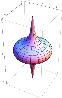
In order to visualize the geometry (71), we can embed it in $\hbox{\mybb R}^{3}$ as a surface of revolution101010This is possible if $L(q_{\text{h}}^{2}-\Delta+l^{2})$ is not too large, since otherwise $(dz/dp)^{2}$ in (75) will become negative in some region.. To this end write the flat metric in cylindrical coordinates,

$$ds_{3}^{2}=dz^{2}+dr^{2}+r^{2}d\phi^{2}\,,$$

and consider $z=z(p)$, $r=r(p)$. Setting $\phi=2\pi y/L$, and identifying the resulting line element with (71), one gets

$$r=\frac{L}{2\pi l}(q_{\text{h}}^{2}-\Delta^{2}+p^{2})^{-1/2}(l^{2}-p^{2})(q_{\text{h}}^{2}-\Delta^{2}+l^{2})\,,$$ (74)

as well as

$$\left(\frac{dr}{dp}\right)^{2}+\left(\frac{dz}{dp}\right)^{2}=\frac{q_{\text{h}}^{2}-\Delta^{2}+p^{2}}{P}\,,$$ (75)

which is a differential equation for $dz/dp$. By expanding near $p=\pm l$, one easily sees that $z$ diverges logarithmically for $|p|\to l$, and that $r$ goes to zero in this limit. We integrated (75) numerically for the values $l=1$, $L=2\pi$ and $q_{\text{h}}^{2}-\Delta^{2}=5$. The resulting surface of revolution is shown in figure 1, where the $z$-axis is vertical. Note that the two cusps extend up to infinity, with $z\to\pm\infty$ for $p\to\pm l$ respectively, while the ‘equator’ $z=0$, where $r$ becomes maximal, is reached for $p=0$.

The metric on the conformal boundary $q\to\infty$ of the black hole solution reads

$$ds_{\text{bdry}}^{2}=-dt^{2}+2dtdy(p^{2}-l^{2})+l^{2}\frac{dp^{2}}{P}\,,$$ (76)

and hence $y$ becomes a lightlike coordinate there.

4 Inclusion of NUT- and electric charges

Inspired by the solution in section 5 of Chong:2004na , we make the following ansatz to include also NUT- and electric charges:

$$ds^{2}=-\frac{Q}{W}\left[dt-p_{1}p_{2}dy\right]^{2}+\frac{P}{W}\left[dt+q_{1}q_{2}dy\right]^{2}+W\left(\frac{dq^{2}}{Q}+\frac{dp^{2}}{P}\right)\,,$$ (77)

where $Q,P$ are again given by (32) (with $a_{4}=b_{4}=1/l^{2}$), and

$$W=q_{1}q_{2}+p_{1}p_{2}\,,\qquad q_{1}=q-\Delta\,,\qquad q_{2}=q+\Delta\,,\qquad p_{1}=p-\delta\,,\qquad p_{2}=p+\delta\,.$$

The ansatz for the gauge potentials and the scalars is

$$A^{\Lambda}=\frac{\mathsf{P}^{\Lambda}(dt+q_{1}q_{2}dy)}{W}p_{1}+\frac{\mathsf{Q}^{\Lambda}(dt-p_{1}p_{2}dy)}{W}q_{1}\,,$$ (78)
$$\tau=e^{-\varphi}+i\chi=\frac{X^{1}}{X^{0}}=\frac{\mu W+i(\nu p+\lambda q)}{q_{1}^{2}+p_{1}^{2}}\,,$$ (79)

where the constants $\mathsf{Q}^{\Lambda}$ are proportional to the electric charges, and $\mu,\nu,\lambda$ are constants to be determined.

We have checked that the equations of motion of the $F=-iX^{0}X^{1}$ model are satisfied if the parameters assume the following form:

$$a_{4}=b_{4}=1/l^{2}\,,$$ (80)
$${}a_{0}=b_{0}-a_{2}\Delta^{2}-\frac{\Delta^{4}}{l^{2}}+\frac{g_{0}{\mathsf{P}^{0}}^{2}}{2g_{1}}+\frac{g_{1}{\mathsf{P}^{1}}^{2}}{2g_{0}}+\frac{g_{0}{\mathsf{Q}^{0}}^{2}}{2g_{1}}+\frac{g_{1}{\mathsf{Q}^{1}}^{2}}{2g_{0}}+$$
$$-\frac{a_{2}\Delta^{2}{\mathsf{Q}^{1}}^{2}}{{\mathsf{P}^{1}}^{2}}-\frac{2\Delta^{4}{\mathsf{Q}^{1}}^{2}}{l^{2}\,{\mathsf{P}^{1}}^{2}}-\frac{\Delta^{4}{\mathsf{Q}^{1}}^{4}}{l^{2}\,{\mathsf{P}^{1}}^{4}}\,,$$ (81)
$$b_{1}=-\frac{2l^{2}\mathsf{P}^{1}(g_{0}^{2}(-2\mathsf{P}^{0}\mathsf{P}^{1}\mathsf{Q}^{0}+{\mathsf{P}^{0}}^{2}\mathsf{Q}^{1}-{\mathsf{Q}^{0}}^{2}\mathsf{Q}^{1})+g_{1}^{2}\mathsf{Q}^{1}({\mathsf{P}^{1}}^{2}+{\mathsf{Q}^{1}}^{2}))}{\Delta({\mathsf{P}^{1}}^{2}+{\mathsf{Q}^{1}}^{2})}\,,$$ (82)
$$a_{1}=-\frac{2l^{2}\mathsf{P}^{1}(g_{0}^{2}(-{\mathsf{P}^{0}}^{2}\mathsf{P}^{1}+\mathsf{P}^{1}{\mathsf{Q}^{0}}^{2}-2\mathsf{P}^{0}\mathsf{Q}^{0}\mathsf{Q}^{1})+g_{1}^{2}\mathsf{P}^{1}({\mathsf{P}^{1}}^{2}+{\mathsf{Q}^{1}}^{2}))}{\Delta({\mathsf{P}^{1}}^{2}+{\mathsf{Q}^{1}}^{2})}\,,$$ (83)
$$b_{2}=-a_{2}-\frac{2\Delta^{2}({\mathsf{P}^{1}}^{2}+{\mathsf{Q}^{1}}^{2})}{l^{2}\,{\mathsf{P}^{1}}^{2}}\,,$$ (84)
$$\mu=\frac{g_{0}}{g_{1}}\,,\qquad\nu=\frac{2\Delta g_{0}}{g_{1}}\,,\qquad\lambda=\frac{2\Delta g_{0}\mathsf{Q}^{1}}{g_{1}\mathsf{P}^{1}}\,,\qquad\delta=-\frac{\Delta\mathsf{Q}^{1}}{\mathsf{P}^{1}}\,.$$ (85)

The solution has free parameters $\Delta$, $b_{0}$ $a_{2}$, $\mathsf{P}^{\Lambda}$ and $\mathsf{Q}^{\Lambda}$. It reduces to the one we have previously found for $\mathsf{Q}^{1}=0=\mathsf{Q}^{0}$.

Let us now keep the ansatz (77)-(78) for the metric and the gauge fields and look for a solution with a scalar field of the form

$$\tau=e^{-\varphi}+i\chi=\frac{X^{1}}{X^{0}}=\frac{\mu W+i(\nu p+\lambda q)}{q_{2}^{2}+p_{2}^{2}}\,.$$ (86)

In this case, the equations of motions are satisfied for the following parameters

$$a_{4}=b_{4}=1/l^{2}\,,$$ (87)
$${}a_{0}=b_{0}-a_{2}\Delta^{2}-\frac{\Delta^{4}}{l^{2}}+\frac{g_{0}{\mathsf{P}^{0}}^{2}}{2g_{1}}+\frac{g_{1}{\mathsf{P}^{1}}^{2}}{2g_{0}}+\frac{g_{0}{\mathsf{Q}^{0}}^{2}}{2g_{1}}+\frac{g_{1}{\mathsf{Q}^{1}}^{2}}{2g_{0}}+$$
$$-\frac{a_{2}\Delta^{2}{\mathsf{Q}^{0}}^{2}}{{\mathsf{P}^{0}}^{2}}-\frac{2\Delta^{4}{\mathsf{Q}^{0}}^{2}}{l^{2}\,{\mathsf{P}^{0}}^{2}}-\frac{\Delta^{4}{\mathsf{Q}^{0}}^{4}}{l^{2}\,{\mathsf{P}^{0}}^{4}}\,,$$ (88)
$$b_{1}=-\frac{2l^{2}\mathsf{P}^{0}(g_{1}^{2}(-2\mathsf{P}^{1}\mathsf{P}^{0}\mathsf{Q}^{1}+{\mathsf{P}^{1}}^{2}\mathsf{Q}^{0}-{\mathsf{Q}^{1}}^{2}\mathsf{Q}^{0})+g_{0}^{2}\mathsf{Q}^{0}({\mathsf{P}^{0}}^{2}+{\mathsf{Q}^{0}}^{2}))}{\Delta({\mathsf{P}^{0}}^{2}+{\mathsf{Q}^{0}}^{2})}\,,$$ (89)
$$a_{1}=-\frac{2l^{2}\mathsf{P}^{0}(g_{1}^{2}(-{\mathsf{P}^{1}}^{2}\mathsf{P}^{0}+\mathsf{P}^{0}{\mathsf{Q}^{1}}^{2}-2\mathsf{P}^{1}\mathsf{Q}^{0}\mathsf{Q}^{1})+g_{0}^{2}\mathsf{P}^{0}({\mathsf{P}^{0}}^{2}+{\mathsf{Q}^{0}}^{2}))}{\Delta({\mathsf{P}^{0}}^{2}+{\mathsf{Q}^{0}}^{2})}\,,$$ (90)
$$b_{2}=-a_{2}-\frac{2\Delta^{2}({\mathsf{P}^{0}}^{2}+{\mathsf{Q}^{0}}^{2})}{l^{2}\,{\mathsf{P}^{0}}^{2}}\,,$$ (91)
$$\mu=\frac{g_{0}}{g_{1}}\,,\qquad\nu=-\frac{2\Delta g_{0}}{g_{1}}\,,\qquad\lambda=-\frac{2\Delta g_{0}\mathsf{Q}^{0}}{g_{1}\mathsf{P}^{0}}\,,\qquad\delta=-\frac{\Delta\mathsf{Q}^{0}}{\mathsf{P}^{0}}\,.$$ (92)

One can easily check that the two ansätze (79) and (86) (when expressed in terms of the parameters $\Delta$ and $\delta$) are related by the strong-weak coupling transformation

$$\tau\to\frac{g_{0}^{2}}{g_{1}^{2}\tau}\,.$$ (93)

This is actually a residual $\hbox{\mybb Z}_{2}$ symmetry of the full symplectic group $\text{Sp}(4,\hbox{\mybb R})$ that remains after the gauging, corresponding to a reparametrization of the scalar manifold, given by the action of the matrix

$${\cal S}=\left(\begin{array}[]{cc}A&B\\ C&D\end{array}\right)\in\text{Sp}(4,\hbox{\mybb R})\,,$$ (94)

with $B=C=0$,

$$A=\left(\begin{array}[]{cc}0&g_{1}/g_{0}\\ g_{0}/g_{1}&0\end{array}\right)\,,$$ (95)

and $D=(A^{-1})^{T}$. Since ${\cal S}^{2}=\hbox{\mybb I}$, it generates $\hbox{\mybb Z}_{2}$, as stated. Notice also that the scalar potential is invariant under (93). Moreover, the matrix (94) acts on the charges by interchanging $g_{0}\mathsf{P}^{0}\leftrightarrow g_{1}\mathsf{P}^{1}$ and $g_{0}\mathsf{Q}^{0}\leftrightarrow g_{1}\mathsf{Q}^{1}$, which is exactly what transforms (81)-(85) to the new parameters (88)-(92).

In order to discuss more in detail the solution (80)-(85), we assume that the polynomial $P$ has four distinct roots $p_{a}<p_{b}<p_{c}<p_{d}$. Since we are interested in black holes with compact horizon111111Black holes with hyperbolic horizons can be obtained by taking the region $p\geq p_{d}$., we consider the region $p_{b}\leq p\leq p_{c}$ (where $P$ is positive), and set $p=N+j\cos\theta$, where

$$N\equiv\frac{p_{b}+p_{c}}{2}\,,\qquad j\equiv\frac{p_{c}-p_{b}}{2}\,,$$ (96)

and $0\leq\theta\leq\pi$. Using the scaling symmetry (40), supplemented by

$$\delta\to\lambda\delta\,,\qquad b_{1}\to\lambda^{3}b_{1}\,,$$

one can set $p_{d}=-N+\sqrt{l^{2}+4N^{2}}$ without loss of generality121212This choice is made in order to correctly reproduce the KNTN-AdS solution of minimal gauged supergravity as a special subcase, see e.g. AlonsoAlberca:2000cs .. This implies

$$b_{0}=(j^{2}-N^{2})\left(1+\frac{3N^{2}}{l^{2}}\right)\,,\quad b_{1}=2N\left(1-\frac{j^{2}}{l^{2}}+\frac{4N^{2}}{l^{2}}\right)\,,\quad b_{2}=-1-\frac{j^{2}}{l^{2}}-\frac{6N^{2}}{l^{2}}\,,$$
$$a_{0}=b_{0}+b_{2}(\Delta^{2}+\delta^{2})+\frac{(\Delta^{2}+\delta^{2})^{2}}{l^{2}}+2l^{2}\left[g_{0}^{2}({\mathsf{P}^{0}}^{2}+{\mathsf{Q}^{0}}^{2})+g_{1}^{2}({\mathsf{P}^{1}}^{2}+{\mathsf{Q}^{1}}^{2})\right]\,,$$
$$a_{2}=1+\frac{j^{2}}{l^{2}}+\frac{6N^{2}}{l^{2}}-\frac{2}{l^{2}}(\Delta^{2}+\delta^{2})\,.$$ (97)

Taking also

$$t\to t+\left(\frac{j}{\Xi}+\frac{N^{2}-\delta^{2}}{j\Xi}\right)\phi\,,\qquad y\to\frac{\phi}{j\Xi}\,,$$

the metric (77) becomes

$\displaystyle ds^{2}=$ $\displaystyle-\frac{Q}{q^{2}-\Delta^{2}+(N+j\cos\theta)^{2}-\delta^{2}}\left[dt+\frac{j\sin^{2}\!\theta}{\Xi}d\phi-\frac{2N}{\Xi}\cos\theta d\phi\right]^{2}$
$\displaystyle+\,\left[q^{2}-\Delta^{2}+(N+j\cos\theta)^{2}-\delta^{2}\right]\left(\frac{dq^{2}}{Q}+\frac{d\theta^{2}}{\Delta_{\theta}}\right)$
$\displaystyle+\,\frac{\Delta_{\theta}\sin^{2}\!\theta}{q^{2}-\Delta^{2}+(N+j\cos\theta)^{2}-\delta^{2}}\left[jdt+\frac{q^{2}+j^{2}+N^{2}-\Delta^{2}-\delta^{2}}{\Xi}d\phi\right]^{2}\,,$

where now

$$\Delta_{\theta}=1-\frac{j^{2}}{l^{2}}\cos^{2}\!\theta-\frac{4Nj}{l^{2}}\cos\theta\,,$$

while the fluxes and the scalar field are given respectively by

$\displaystyle F^{\Lambda}$ $\displaystyle=$ $\displaystyle\frac{\mathsf{P}^{\Lambda}(q^{2}-\Delta^{2}-(p-\delta)^{2})-2(q-\Delta)p\mathsf{Q}^{\Lambda}}{\left[q^{2}-\Delta^{2}+(N+j\cos\theta)^{2}-\delta^{2}\right]^{2}}\sin\theta\left[jdt+\frac{q^{2}+j^{2}+N^{2}-\Delta^{2}-\delta^{2}}{\Xi}d\phi\right]\wedge d\theta$
$\displaystyle+$ $\displaystyle\frac{\mathsf{Q^{\Lambda}}(p^{2}-\delta^{2}-(q-\Delta)^{2})-2(p-\delta)q\mathsf{P}^{\Lambda}}{\left[q^{2}-\Delta^{2}+(N+j\cos\theta)^{2}-\delta^{2}\right]^{2}}dq\wedge\left[dt+\frac{j\sin^{2}\!\theta}{\Xi}d\phi-\frac{2N}{\Xi}\cos\theta d\phi\right]\,,$
$$\tau=\frac{g_{0}}{g_{1}}\frac{q+\Delta-i(p+\delta)}{q-\Delta-i(p-\delta)}\,,$$

with $p=N+j\cos\theta$.

If one turns off the rotation ($j=0$), and fixes the charges in terms of $N,\Delta,\delta$ according to

$$g_{1}\mathsf{P}^{1}=\frac{N^{2}}{l^{2}}-\frac{N\delta}{l^{2}}+\frac{1}{4}\,,\quad g_{1}\mathsf{Q}^{1}=-\frac{\delta}{\Delta}g_{1}\mathsf{P}^{1}\,,\quad g_{0}\mathsf{P}^{0}=g_{1}\mathsf{P}^{1}+\frac{2N\delta}{l^{2}}\,,\quad g_{0}\mathsf{Q}^{0}=g_{1}\mathsf{Q}^{1}+\frac{2N\Delta}{l^{2}}\,,$$

one recovers the spherical NUT-charged BPS solution constructed in Colleoni:2012jq 131313The flat or hyperbolic BPS solutions of Colleoni:2012jq can be obtained in a similar way. Notice that only the latter represent genuine black holes, while in the spherical or flat case one has naked singularities Colleoni:2012jq .. With the charges fixed as above, and

$$a_{1}=-\frac{4N}{\Delta}\left[\frac{2N\delta^{2}}{l^{2}}+\frac{2N\Delta^{2}}{l^{2}}-\frac{2N^{2}\delta}{l^{2}}-\frac{\delta}{2}\right]\,,$$

all the constraints (81)-(84) are satisfied.

From (4), we can also get a dyonic solution without NUT charge. Setting $N=0$ one has

$$b_{0}=j^{2}\,,\qquad b_{1}=0\,,\qquad b_{2}=-1-\frac{j^{2}}{l^{2}}\,,\qquad a_{2}=1+\frac{j^{2}}{l^{2}}-\frac{2}{l^{2}}(\Delta^{2}+\delta^{2})\,,$$
$$a_{0}=j^{2}-\left(1+\frac{j^{2}}{l^{2}}\right)(\Delta^{2}+\delta^{2})+\frac{(\Delta^{2}+\delta^{2})^{2}}{l^{2}}+2l^{2}\left[g_{0}^{2}({\mathsf{P}^{0}}^{2}+{\mathsf{Q}^{0}}^{2})+g_{1}^{2}({\mathsf{P}^{1}}^{2}+{\mathsf{Q}^{1}}^{2})\right]\,,$$

and $a_{1}$ is given by (83). Since $b_{1}$ vanishes, (82) implies $\mathsf{P}^{1}=0$ or

$$g_{0}^{2}\left(\mathsf{Q}^{0}\mathsf{Q}^{1}+\mathsf{P}^{0}\mathsf{P}^{1}\right)^{2}=\left({\mathsf{Q}^{1}}^{2}+{\mathsf{P}^{1}}^{2}\right)\left(g_{1}^{2}{\mathsf{Q}^{1}}^{2}+g_{0}^{2}{\mathsf{P}^{0}}^{2}\right)\,,$$ (99)

which allows to express e.g. $\mathsf{Q}^{0}$ in terms of the other charges. The solution is thus specified by the five parameters $\mathsf{P}^{0},\mathsf{P}^{1},\mathsf{Q}^{1},j,\Delta$, or alternatively by three charges, angular momentum and mass.

Note that, also in the case with nonvanishing $N$, (82) together with the second eqn. in (97) fix one of the electromagnetic charges in terms of the other parameters, and therefore the solution is labelled by three independent $\text{U}(1)$ charges, NUT charge, angular momentum and mass. It is thus not the most general solution, which should have four independent $\text{U}(1)$ charges.

4.1 Solution with harmonic functions and flat limit

We can partially rewrite the ansatz in terms of complex harmonic functions in order to make the dependence on the prepotential more suggestive. If we define the variable $\rho=q-ip$, we can use the harmonic functions in $\rho$,

$$X^{0}\equiv H_{0}=h_{0}(1-\frac{\Delta-i\delta}{\rho})\ ,\qquad X^{1}\equiv H_{1}=h_{1}(1+\frac{\Delta-i\delta}{\rho})\ ,$$ (100)

with $h_{0}=g_{0}^{-1},h_{1}=g_{1}^{-1}$. We can then rewrite the scalar ansatz as

$$\tau=\frac{H_{1}}{H_{0}}\,,$$ (101)

while the function $W$ appearing in the metric and gauge field ansätze (77), (78) can be cast into the form

$$W=l^{2}(q^{2}+p^{2})e^{-K(X^{\Lambda})}\ ,$$ (102)

where $K$ is the Kähler potential of special geometry that depends on the prepotential141414Note that here we do not mean the physical Kähler potential $K(\tau,\bar{\tau})$, but the one that is obtained directly from the sections (100).. In the case of $F=-iX^{0}X^{1}$, we have

$$e^{-K}_{F=-iX^{0}X^{1}}=\frac{1}{l^{2}(q^{2}+p^{2})}(q_{1}q_{2}+p_{1}p_{2})\ ,$$ (103)

as needed.

Rewriting the solution in this form makes it easy to take the limit of vanishing gauging. We take $g_{0},g_{1}\rightarrow 0$, keeping the ratio an arbitrary finite constant (which is the value of the scalar field at infinity). This leads to a simplification in the explicit parameters $a_{i},b_{i}$ that parametrize the functions $P(p)$ and $Q(q)$. We can again write the metric in the form (4), but now with $\Delta_{\theta}=\Xi=1$. A further redefinition of the radial coordinate $q=r+m$ for $a_{1}=-2m$ leads to

$$Q=r^{2}+(j^{2}+m^{2}-N^{2}-\Delta^{2}-\delta^{2})\ .$$

Written this way, the solution can be seen to sit inside the general class of solutions of LozanoTellechea:1999my with arbitrary mass, angular momentum, electric and magnetic and NUT charges. Just like in the case with cosmological constant, we cannot recover the most general class due to the restriction that the NUT charge is fixed in terms of the electric and magnetic charges, c.f. (82) and (97).

5 Final remarks and outlook

Given the various examples and solutions we presented in the preceeding sections, we can make an ansatz that is likely to yield solutions for more general prepotentials with arbitrary number of vector multiplets. The metric ansatz would remain

$$ds^{2}=-f(dt+\omega_{y}dy)^{2}+f^{-1}\left[v\left(\frac{dq^{2}}{Q}+\frac{dp^{2}}{P}\right)+PQdy^{2}\right]\,,$$ (104)

with

$$Q=a_{0}+a_{1}q+a_{2}q^{2}+g^{2}q^{4}\,,\quad P=b_{0}+b_{1}p+b_{2}p^{2}+g^{2}p^{4}\,,\quad v=Q-P\ ,\quad f=ve^{2U}\ ,$$ (105)
$$e^{-2U}=i(\overline{X}^{\Lambda}F_{\Lambda}-X^{\Lambda}\overline{F}_{\Lambda})\ ,\quad\omega_{y}=-\frac{1}{v}\left(Q(c_{0}+c_{1}p+p^{2})+P(d_{0}+d_{1}q+q^{2})\right)\ ,$$ (106)

scalar fields given by the symplectic sections

$$X^{\Lambda}=h^{\Lambda}(q-ip+\Delta^{\Lambda}-i\delta^{\Lambda})\ ,$$ (107)

and gauge fields

$\displaystyle A^{\Lambda}$ $\displaystyle=$ $\displaystyle\frac{1}{W}\left(\mathsf{P}^{\Lambda}(p+k_{0})({\rm d}t+(d_{0}+d_{1}q+q^{2}){\rm d}y)\right.$ (108)
$\displaystyle+\left.\mathsf{Q}^{\Lambda}(q+l_{0})({\rm d}t-(c_{0}+c_{1}p+p^{2}){\rm d}y)\right)\ .$

The real constant parameters $a_{0},a_{1},a_{2},b_{0},b_{1},b_{2},c_{0},c_{1},d_{0}.d_{1},k_{0},l_{0},h^{\Lambda},\Delta^{\Lambda},\delta^{\Lambda},P^{\Lambda},Q^{\Lambda}$ will eventually have to be expressed in terms of the physical parameters of a given solution (mass, angular momentum, NUT charge, electric and magnetic charges) upon solving the equations of motion in a chosen model. The question whether the above ansatz leads to solutions in models of the STU type is left for future research.

Acknowledgements.
We would like to thank S. Katmadas, A. Tomasiello and S. Vandoren for interesting discussions. A.G. and C.T. would also like to thank Università degli Studi di Milano and Milano-Bicocca for the kind hospitality during various visits, while this work was in progress. A.G. and C.T. acknowledge support by the Netherlands Organization for Scientific Research (NWO) under the VICI grant 680-47-603. K.H. is supported in part by INFN and by the MIUR-FIRB grant RBFR10QS5J “String Theory and Fundamental Interactions”. The work of D.K. was partially supported by INFN and MIUR-PRIN contract 2009-KHZKRX. The work of O.V. is supported by the German Science Foundation (DFG) under the Collaborative Research Center (SFB) 676 “Particles, Strings and the Early Universe”.

Appendix A 1/2 BPS near-horizon geometries

An interesting class of half-supersymmetric backgrounds was obtained in Klemm:2010mc . It includes the near-horizon geometry of extremal rotating black holes. The metric and the fluxes read respectively

$\displaystyle ds^{2}$ $\displaystyle=$ $\displaystyle-z^{2}e^{\xi}\left[dt+4(e^{-2\xi}-L)\frac{dx}{z}\right]^{2}+4e^{-\xi}\frac{dz^{2}}{z^{2}}$ (109)
$\displaystyle\qquad+16e^{-\xi}(e^{-2\xi}-L)dx^{2}+\frac{4e^{-2\xi}d\xi^{2}}{Y^{2}(e^{-\xi}-Le^{\xi})}\ ,$
$\displaystyle F^{\Lambda}$ $\displaystyle=$ $\displaystyle 8i\left(\frac{\bar{X}L^{\Lambda}}{1-iY}-\frac{X\bar{L}^{\Lambda}}{1+iY}\right)dt\wedge dz$
$\displaystyle+\frac{4}{Y}\left[\frac{2\bar{X}L^{\Lambda}}{1-iY}+\frac{2X\bar{L}^{\Lambda}}{1+iY}+\left(\mbox{Im}\,\mathcal{N}\right)^{-1|\Lambda\Sigma}g_{\Sigma}\right](zdt-4Ldx)\wedge d\xi\ ,$

where $L$ is a real integration constant, $X\equiv g_{\Lambda}L^{\Lambda}$, and $Y$ is defined by

$$Y^{2}=64e^{-\xi}|X|^{2}-1\ .$$ (111)

The moduli fields $z^{\alpha}$ depend on the coordinate $\xi$ only, and obey the differential equation

$$\frac{dz^{\alpha}}{d\xi}=\frac{i}{2\bar{X}Y}(1-iY)g^{\alpha\bar{\beta}}{\cal D}_{\bar{\beta}}\bar{X}\ .$$ (112)

For $L>0$, the line element (109) can be cast into the simple form

$\displaystyle ds^{2}$ $\displaystyle=$ $\displaystyle 4e^{-\xi}\left(-z^{2}d{\hat{t}}^{2}+\frac{dz^{2}}{z^{2}}\right)+16L(e^{-\xi}-Le^{\xi})\left(dx-\frac{z}{2\sqrt{L}}d\hat{t}\right)^{2}$ (113)
$\displaystyle\qquad+\frac{4e^{-2\xi}d\xi^{2}}{Y^{2}(e^{-\xi}-Le^{\xi})}\ ,$

where $\hat{t}\equiv t/(2\sqrt{L})$. (113) is of the form (3.3) of Astefanesei:2006dd , and describes the near-horizon geometry of extremal rotating black holes151515Metrics of the type (113) were discussed for the first time in Bardeen:1999px in the context of the extremal Kerr throat geometry., with isometry group $\text{SL}(2,\hbox{\mybb R})\times\text{U}(1)$. From (112) it is clear that the scalar fields have a nontrivial dependence on the horizon coordinate $\xi$ unless $g_{\Lambda}{\cal D}_{\alpha}X^{\Lambda}=0$. As was shown in Klemm:2010mc , the solution with constant scalars is the near-horizon limit of the supersymmetric rotating hyperbolic black holes in minimal gauged supergravity Caldarelli:1998hg . Moreover, in Klemm:2011xw , a class of rotating BPS black holes with running scalar was constructed for the prepotential $F=-iX^{0}X^{1}$, which has again (113) as near-horizon limit.

Let us first consider the case of gauged supergravity with flat scalar potential $V$, that was studied recently in Hristov:2012nu . The condition $V=0$ translates into

$${\cal D}_{\alpha}Xg^{\alpha\bar{\beta}}{\cal D}_{\bar{\beta}}\bar{X}=3|X|^{2}\,.$$ (114)

Now, using (112), it is straightforward to show that

$$\frac{d|X|^{2}}{d\xi}={\cal D}_{\alpha}Xg^{\alpha\bar{\beta}}{\cal D}_{\bar{\beta}}\bar{X}\,.$$ (115)

Using (114), this can be integrated to give

$$|X|^{2}=C^{2}e^{3\xi}\,,$$ (116)

where $C$ denotes an integration constant. Then, (111) allows to express $\xi$ in terms of $Y$,

$$e^{-\xi}=8C(Y^{2}+1)^{-1/2}\,.$$ (117)

In asymptotically flat space, there are underrotating black holes Rasheed:1995zv , whose near-horizon geometry is given by

$$ds^{2}=-e^{2U}r^{2}(dt+\omega)^{2}+e^{-2U}\left(\frac{dr^{2}}{r^{2}}+d\theta^{2}+\sin^{2}\theta d\phi^{2}\right)\,,$$ (118)

where

$$e^{-4U}=-I_{4}-j^{2}\cos^{2}\theta\,,\qquad\omega=j\frac{\sin^{2}\theta}{r}d\phi\,,$$ (119)

$j$ is the rotation parameter and $I_{4}$ denotes the quartic invariant of the charges. It turns out that (118) is actually a one-half BPS solution of gauged supergravity (with flat potential). To see this, choose $C=|I_{4}|^{1/2}/32$ (we need $I_{4}<0$), $L=(|I_{4}|-j^{2})/16$, and make the coordinate transformation

$$z=\frac{r}{2}\,,\qquad x=\frac{2\phi}{j}\,,\qquad e^{-\xi}=\frac{1}{4}e^{-2U}\,,$$ (120)

that casts (109) into (118). (Use also (117) to eliminate $Y$ in favour of $\xi$). In Hristov:2012nu it was shown that the underrotating near-horizon geometry (118) preserves at least one quarter of the supersymmetries, but it was not excluded that it is even 1/2 BPS (cf. footnote 14 of Hristov:2012nu ). Here we showed that this is indeed the case.

In the case of the model with prepotential $F=-iX^{0}X^{1}$, the general solution of the differential equation (112) was found in Klemm:2011xw , and is given by

$$\tau=\frac{X^{1}}{X^{0}}=\frac{g_{0}}{g_{1}}\frac{Y-i+C}{Y-i-C}\,,$$ (121)

where $C$ denotes a complex integration constant. We shall now obtain the conditions under which the near-horizon geometry of the general solution of section 4 fits into this 1/2 BPS class. In the extremal limit, the function $Q$ has a double root at $q=q_{\text{h}}$. Defining new coordinates $z,\hat{t},\hat{y}$ by

$$q=q_{\text{h}}+\epsilon q_{0}z\,,\quad t=\frac{\hat{t}q_{0}}{\epsilon}\,,\quad y=\hat{y}-\frac{\hat{t}q_{0}}{(q_{\text{h}}^{2}-\Delta^{2})\epsilon}\,,\quad q_{0}^{2}\equiv\frac{q_{\text{h}}^{2}-\Delta^{2}}{\hat{C}}\,,\quad\hat{C}\equiv a_{2}+\frac{6q_{\text{h}}^{2}}{l^{2}}\,,$$

and taking $\epsilon\to 0$ with $z,\hat{t},\hat{y}$ fixed, we get the near-horizon limit of (77), (79) and the field strength following from (78),

$$ds^{2}=\frac{W_{\text{h}}}{\hat{C}}\left(-z^{2}d\hat{t}^{2}+\frac{dz^{2}}{z^{2}}\right)+\frac{W_{\text{h}}dp^{2}}{P}+\frac{P}{W_{\text{h}}}\left((q_{\text{h}}^{2}-\Delta^{2})d\hat{y}-\frac{2q_{\text{h}}z}{\hat{C}}d\hat{t}\right)^{2}\,,$$ (122)
$$\tau=\frac{g_{0}}{g_{1}}\frac{q_{\text{h}}+\Delta-i(p+\delta)}{q_{\text{h}}-\Delta-i(p-\delta)}\,,$$ (123)
$\displaystyle F^{\Lambda}$ $\displaystyle=$ $\displaystyle\frac{\mathsf{P}^{\Lambda}((p-\delta)^{2}-q_{\text{h}}^{2}+\Delta^{2})+2p\mathsf{Q}^{\Lambda}(q_{\text{h}}-\Delta)}{W_{\text{h}}^{2}}\left[(q_{\text{h}}^{2}-\Delta^{2})d\hat{y}-\frac{2q_{\text{h}}z}{\hat{C}}d\hat{t}\right]\wedge dp$ (124)
$\displaystyle\quad+\frac{\mathsf{Q}^{\Lambda}((q_{\text{h}}-\Delta)^{2}-p^{2}+\delta^{2})+2q_{\text{h}}\mathsf{P}^{\Lambda}(p-\delta)}{W_{\text{h}}\hat{C}}d\hat{t}\wedge dz\,,$

where $W_{\text{h}}\equiv q^{2}_{\text{h}}-\Delta^{2}+p^{2}-\delta^{2}$. This coincides with (113), (121) and (A) respectively if the following constraints hold:

$$Q=\frac{1}{l^{2}}(q^{2}-q_{\text{h}}^{2})^{2}\,,\qquad\mathsf{Q}^{\Lambda}=\delta=0\,,\qquad\mathsf{P}^{\Lambda}=\frac{8q_{\text{h}}^{2}}{l^{4}g_{\Lambda}}\sqrt{L}\,.$$ (125)

The coordinates $\hat{y}$ and $p$ are related to $x$ and $\xi$ in (113) by

$$\hat{y}=\frac{l^{2}\sqrt{L}}{q_{\text{h}}(q_{\text{h}}^{2}-\Delta^{2})}x\,,\qquad e^{\xi}=\frac{16q_{\text{h}}^{2}}{l^{2}W_{\text{h}}}\,,$$ (126)

while the constant $C$ in (121) is given by $C=-i\Delta/q_{\text{h}}$, and $Y=-p/q_{\text{h}}$. Since the location of the horizon can be set to $q_{\text{h}}=l$ without loss of generality by using the scaling symmetry (40), the 1/2 BPS near-horizon geometry is specified in terms of the two parameters $\Delta$ (or alternatively $C$) and $L$. Note that this solution was first constructed in Klemm:2011xw . Since (A), (113) and (121) do not exhaust all possible half-supersymmetric solutions, the results of this appendix do not necessarily imply that there are no further 1/2 BPS subclasses of (77)-(79).

Appendix B Real formulation of special geometry

Here we will present three dimensional effective Lagrangian for stationary field configurations, adapted to the real formulation of special geometry. In the ungauged case, the resulting three-dimensional Lagrangian, which takes the form of a non-linear sigma model, was constructed in Mohaupt:2011aa (see eq (29)). For the case of gauged supergravity one must add an additional Fayet-Iliopoulos potential

$\displaystyle\begin{aligned} \texttt{e}^{-1}_{3}{\cal L}_{3}=\;\;&\frac{1}{2}R_{3}-\tilde{H}_{ab}\left(\partial q^{a}\partial q^{b}-\partial\hat{q}^{a}\partial\hat{q}^{b}\right)+\frac{1}{2H}V(q)\\ &-\frac{1}{H^{2}}\left(q^{a}\Omega_{ab}\partial q^{b}\right)^{2}+\frac{2}{H^{2}}\left(q^{a}\Omega_{ab}\partial\hat{q}^{b}\right)^{2}\\ &-\frac{1}{4H^{2}}\left(\partial\tilde{\phi}+2\hat{q}^{a}\Omega_{ab}\partial\hat{q}^{b}\right)^{2}\;,\end{aligned}$ (127)

where $\tilde{H}_{ab}=-\frac{1}{2}\frac{\partial^{2}}{\partial q^{a}\partial q^{b}}\log(-2H)$. The Lagrangian is completely determined by specifying a Hesse potential $H$, which plays the an analogous role to the holomorphic prepotential when using special real coordinates. In Klemm:2012yg ; Klemm:2012vm static solutions were considered for which the second and third lines of the above Lagrangian can be consistently set to zero. In this paper we are interested in NUT charged and rotating solutions in which case all terms become relevant.

The fields appearing in (127) are related to the complex scalar fields and gauge fields appearing in the main text by the following dictionary:

$\displaystyle q^{a}$ $\displaystyle:=\left(\begin{array}[]{c}x^{\Lambda}\\ y_{\Lambda}\end{array}\right):=\left(\begin{array}[]{c}e^{\phi/2}\text{Re}L^{\Lambda}\\ e^{\phi/2}\text{Re}M_{\Lambda}\end{array}\right)\;,$ (132)
$\displaystyle\partial_{m}\hat{q}^{a}$ $\displaystyle:=\left(\begin{array}[]{c}\frac{1}{2}\partial_{m}\zeta^{\Lambda}\\ \frac{1}{2}\partial_{m}\tilde{\zeta}_{\Lambda}\end{array}\right):=\left(\begin{array}[]{c}\frac{1}{2}F^{\Lambda}_{m0}\\ \frac{1}{2}G_{\Lambda|m0}\end{array}\right)\;,$ (137)
$\displaystyle\left(\partial_{m}\tilde{\phi}+2\hat{q}^{a}\Omega_{ab}\partial_{m}\hat{q}^{b}\right)$ $\displaystyle:=2H^{2}\varepsilon_{m}^{\;\;\;nr}\partial_{[n}\omega_{r]}\;,$ (138)

whilst the three- and four-dimensional metrics satisfy the expression

$$g_{4}=-e^{\phi}(dt+\omega_{m}dx^{m})^{2}+e^{-\phi}g_{3}\;.$$ (139)

The Hesse potential is related to the Fayet–Iliopoulos potential $V$ through expression (A.2) of Klemm:2012yg , and to the KK-scalar through $-2H=e^{\phi}$.

B.1 Equations of motion

For future reference it will be convenient to write down the full equations of motion of the three-dimensional effective Lagrangian (127).

We first perform the variation with respect to the $q^{a}$ fields, which results in the equations

$\displaystyle\begin{aligned} &2\nabla^{m}\left[\tilde{H}_{ab}\partial_{m}q^{b}\right]-\partial_{a}\tilde{H}_{bc}\left(\partial_{m}q^{b}\partial^{m}q^{c}-\partial_{m}\hat{q}^{b}\partial^{m}\hat{q}^{c}\right)+\partial_{a}\left(\frac{1}{2H}V(q)\right)\\ &+2\nabla^{m}\left[\frac{1}{H^{2}}q^{c}\Omega_{ca}\left(q^{d}\Omega_{de}\partial_{m}q^{e}\right)\right]\\ &-2\partial_{a}\left(\frac{1}{H}q^{c}\right)\left[\Omega_{cb}\partial_{m}q^{b}\frac{1}{H}\left(q^{d}\Omega_{de}\partial^{m}q^{e}\right)-2\Omega_{cb}\partial_{m}\hat{q}^{b}\frac{1}{H}\left(q^{d}\Omega_{de}\partial^{m}\hat{q}^{e}\right)\right]\\ &-\partial_{a}\left(\frac{1}{4H^{2}}\right)\left(\partial_{m}\tilde{\phi}+2\hat{q}^{c}\Omega_{cd}\partial_{m}\hat{q}^{d}\right)\left(\partial^{m}\tilde{\phi}+2\hat{q}^{c}\Omega_{cd}\partial^{m}\hat{q}^{d}\right)=0\;.\end{aligned}$ (140)

Next, by varying the $\hat{q}^{a}$ fields we get

$\displaystyle\begin{aligned} &2\nabla^{m}\left[\tilde{H}_{ab}\partial_{m}\hat{q}^{b}\right]\\ &+4\nabla^{m}\left[\frac{1}{H^{2}}q^{c}\Omega_{ca}\left(q^{d}\Omega_{de}\partial_{m}\hat{q}^{e}\right)\right]-\nabla^{m}\left[\frac{1}{H^{2}}\hat{q}^{b}\Omega_{ba}\left(\partial_{m}\tilde{\phi}+2\hat{q}^{c}\Omega_{cd}\partial_{m}\hat{q}^{d}\right)\right]\\ &+\frac{1}{H^{2}}\Omega_{ab}\partial_{m}\hat{q}^{b}\left(\partial^{m}\tilde{\phi}+2\hat{q}^{c}\Omega_{cd}\partial^{m}\hat{q}^{d}\right)=0\;.\end{aligned}$ (141)

The variation of the $\tilde{\phi}$ field, which descends from the Kaluza–Klein vector, gives us simply

$$\nabla^{m}\left[\frac{1}{4H^{2}}\left(\partial_{m}\tilde{\phi}+2\hat{q}^{c}\Omega_{cd}\partial_{m}\hat{q}^{d}\right)\right]=0\;.$$ (142)

Since the dualisation procedure swaps the role of the field equations and Bianchi identities, this equation gives us simply the Bianchi identity for the KK-vector. Finally, from the variation of the three-dimensional metric we obtain the following Einstein equations

$\displaystyle\begin{aligned} &\frac{1}{2}R_{mn}-\tilde{H}_{ab}\left(\partial_{m}q^{a}\partial_{n}q^{b}-\partial_{m}\hat{q}^{a}\partial_{n}\hat{q}^{b}\right)+\frac{1}{2H}g_{mn}V(q)\\ &-\frac{1}{H^{2}}\left(q^{a}\Omega_{ab}\partial_{m}q^{b}\right)\left(q^{c}\Omega_{cd}\partial_{n}q^{d}\right)+\frac{2}{H^{2}}\left(q^{a}\Omega_{ab}\partial_{m}\hat{q}^{b}\right)\left(q^{c}\Omega_{cd}\partial_{n}\hat{q}^{d}\right)\\ &-\frac{1}{4H^{2}}\left(\partial_{m}\tilde{\phi}+2\hat{q}^{a}\Omega_{ab}\partial_{m}\hat{q}^{b}\right)\left(\partial_{n}\tilde{\phi}+2\hat{q}^{c}\Omega_{cd}\partial_{n}\hat{q}^{d}\right)=0\;.\end{aligned}$ (143)

B.2 Example: solution of the $F=-iX^{0}X^{1}$ model

By way of example, we shall present the rotating nonextremal solution of the $F=-iX^{0}X^{1}$ model, as given section 4, in terms of the real formulation of special geometry:

$$g_{3}=v\left(\frac{dq^{2}}{Q}+\frac{dp^{2}}{P}\right)+PQdy^{2}\;,$$
$$q^{a}=\frac{v^{\frac{1}{2}}}{\mu^{\frac{1}{2}}2W}\left(\begin{array}[]{c}\vspace{.5em}q_{1}\\ \vspace{.5em}\dfrac{\mu Wq_{1}-p_{1}(\nu p+\lambda q)}{q_{1}^{2}+p_{1}^{2}}\\ \vspace{.5em}\dfrac{\mu Wp_{1}+q_{1}(\nu p+\lambda q)}{q_{1}^{2}+p_{1}^{2}}\\ \vspace{.5em}p_{1}\end{array}\right),\;\;\;\;\hat{q}^{a}=\frac{1}{2W}\left(\begin{array}[]{c}\vspace{.5em}\mathsf{P}^{0}p_{1}+\mathsf{Q}^{0}q_{1}\\ \vspace{.5em}\mathsf{P}^{1}p_{1}+\mathsf{Q}^{1}q_{1}\\ \vspace{.5em}\mu(\mathsf{P}^{0}q_{2}-\mathsf{Q}^{0}p_{2})\\ \vspace{.5em}\dfrac{1}{\mu}(\mathsf{P}^{1}q_{1}-\mathsf{Q}^{1}p_{1})\\ \end{array}\right),$$
$\displaystyle\frac{1}{H}$ $\displaystyle\left(\partial_{p}\tilde{\phi}+2\hat{q}^{a}\Omega_{ab}\partial_{p}\hat{q}^{b}\right)=-\frac{v}{PW}\partial_{q}\omega_{y}\;,$
$\displaystyle\frac{1}{H}$ $\displaystyle\left(\partial_{q}\tilde{\phi}+2\hat{q}^{a}\Omega_{ab}\partial_{q}\hat{q}^{b}\right)=\frac{v}{QW}\partial_{p}\omega_{y}\;.$

Here the functions $Q,P,W,q_{1},q_{2},p_{1},p_{2}$ and parameters $\mathsf{P}^{\Lambda},\mathsf{Q}^{\Lambda},\mu,\nu,\lambda$ are those that appear in the solution (77) – (85), and the KK-vector is given by

$$\omega_{y}=-\frac{(Pq_{1}q_{2}+Qp_{1}p_{2})}{v}\;,\qquad v=Q-P\;.$$

Using the expression for the Hesse potential (B.1) of Klemm:2012yg , one may explicitly check that the above field configuration solves the equations of motion (140) – (143).

References

  • (1) J. D. Bekenstein, “Black holes and entropy,” Phys. Rev. D 7 (1973) 2333.
  • (2) S. W. Hawking, “Particle creation by black holes,” Commun. Math. Phys.  43 (1975) 199.
  • (3) S. W. Hawking and D. N. Page, “Thermodynamics of black holes in anti-de Sitter space,” Commun. Math. Phys.  87 (1983) 577.
  • (4) S. W. Hawking, C. J. Hunter and M. Taylor, “Rotation and the AdS/CFT correspondence,” Phys. Rev. D 59 (1999) 064005 [hep-th/9811056].
  • (5) A. Chamblin, R. Emparan, C. V. Johnson and R. C. Myers, “Charged AdS black holes and catastrophic holography,” Phys. Rev. D 60 (1999) 064018 [hep-th/9902170].
  • (6) M. Cvetič and S. S. Gubser, “Phases of R-charged black holes, spinning branes and strongly coupled gauge theories,” JHEP 9904 (1999) 024 [hep-th/9902195].
  • (7) A. Chamblin, R. Emparan, C. V. Johnson and R. C. Myers, “Holography, thermodynamics and fluctuations of charged AdS black holes,” Phys. Rev. D 60 (1999) 104026 [hep-th/9904197].
  • (8) M. M. Caldarelli, G. Cognola and D. Klemm, “Thermodynamics of Kerr-Newman-AdS black holes and conformal field theories,” Class. Quant. Grav.  17, 399 (2000) [hep-th/9908022].
  • (9) K. Hristov, C. Toldo and S. Vandoren, “Phase transitions of magnetic AdS4 black holes with scalar hair,” Phys. Rev. D 88 (2013) 026019 [arXiv:1304.5187 [hep-th]].
  • (10) A. Strominger and C. Vafa, “Microscopic origin of the Bekenstein-Hawking entropy,” Phys. Lett. B 379 (1996) 99 [hep-th/9601029].
  • (11) J. M. Maldacena, A. Strominger and E. Witten, “Black hole entropy in M-theory,” JHEP 9712 (1997) 002 [hep-th/9711053].
  • (12) R. Dijkgraaf, E. P. Verlinde and H. L. Verlinde, “Counting dyons in N=4 string theory,” Nucl. Phys. B 484 (1997) 543 [hep-th/9607026].
  • (13) A. Strominger, “Black hole entropy from near horizon microstates,” JHEP 9802 (1998) 009 [hep-th/9712251].
  • (14) S. A. Hartnoll, “Lectures on holographic methods for condensed matter physics,” Class. Quant. Grav.  26 (2009) 224002 [arXiv:0903.3246 [hep-th]].
  • (15) C. P. Herzog, “Lectures on holographic superfluidity and superconductivity,” J. Phys. A 42 (2009) 343001 [arXiv:0904.1975 [hep-th]].
  • (16) J. McGreevy, “Holographic duality with a view toward many-body physics,” Adv. High Energy Phys.  2010 (2010) 723105 [arXiv:0909.0518 [hep-th]].
  • (17) S. Sachdev, “Condensed matter and AdS/CFT,” Lect. Notes Phys.  828 (2011) 273 [arXiv:1002.2947 [hep-th]].
  • (18) S. Barisch, G. Lopes Cardoso, M. Haack, S. Nampuri and N. A. Obers, “Nernst branes in gauged supergravity,” JHEP 1111 (2011) 090 [arXiv:1108.0296 [hep-th]].
  • (19) D. Anninos, T. Anous, F. Denef and L. Peeters, “Holographic vitrification,” arXiv:1309.0146 [hep-th].
  • (20) L. Vanzo, “Black holes with unusual topology,” Phys. Rev. D 56 (1997) 6475 [gr-qc/9705004].
  • (21) M. J. Duff and J. T. Liu, “Anti-de Sitter black holes in gauged N = 8 supergravity,” Nucl. Phys. B 554 (1999) 237 [hep-th/9901149].
  • (22) Z. -W. Chong, M. Cvetič, H. Lu and C. N. Pope, “Charged rotating black holes in four-dimensional gauged and ungauged supergravities,” Nucl. Phys. B 717 (2005) 246 [hep-th/0411045].
  • (23) D. D. K. Chow, “Single-charge rotating black holes in four-dimensional gauged supergravity,” Class. Quant. Grav.  28 (2011) 032001 [arXiv:1011.2202 [hep-th]].
  • (24) D. D. K. Chow, “Two-charge rotating black holes in four-dimensional gauged supergravity,” Class. Quant. Grav.  28 (2011) 175004 [arXiv:1012.1851 [hep-th]].
  • (25) M. M. Caldarelli and D. Klemm, “Supersymmetry of Anti-de Sitter black holes,” Nucl. Phys. B 545 (1999) 434 [hep-th/9808097].
  • (26) N. Alonso-Alberca, P. Meessen and T. Ortín, “Supersymmetry of topological Kerr-Newman-Taub-NUT-AdS space-times,” Class. Quant. Grav.  17 (2000) 2783 [hep-th/0003071].
  • (27) H. Lü, Y. Pang and C. N. Pope, “AdS dyonic black hole and its thermodynamics,” JHEP 1311 (2013) 033 [arXiv:1307.6243 [hep-th]].
  • (28) S. L. Cacciatori and D. Klemm, “Supersymmetric AdS4 black holes and attractors,” JHEP 1001 (2010) 085 [arXiv:0911.4926 [hep-th]].
  • (29) D. Klemm, “Rotating BPS black holes in matter-coupled AdS4 supergravity,” JHEP 1107 (2011) 019 [arXiv:1103.4699 [hep-th]].
  • (30) G. Dall’Agata and A. Gnecchi, “Flow equations and attractors for black holes in N = 2 U(1) gauged supergravity,” JHEP 1103 (2011) 037 [arXiv:1012.3756 [hep-th]].
  • (31) K. Hristov and S. Vandoren, “Static supersymmetric black holes in AdS4 with spherical symmetry,” JHEP 1104 (2011) 047 [arXiv:1012.4314 [hep-th]].
  • (32) N. Halmagyi, M. Petrini and A. Zaffaroni, “BPS black holes in $AdS_{4}$ from M-theory,” JHEP 1308 (2013) 124 [arXiv:1305.0730 [hep-th]].
  • (33) N. Halmagyi, “BPS Black Hole Horizons in N=2 Gauged Supergravity,” arXiv:1308.1439 [hep-th].
  • (34) D. Klemm and O. Vaughan, “Nonextremal black holes in gauged supergravity and the real formulation of special geometry,” JHEP 1301 (2013) 053 [arXiv:1207.2679 [hep-th]].
  • (35) C. Toldo and S. Vandoren, “Static nonextremal AdS4 black hole solutions,” JHEP 1209 (2012) 048 [arXiv:1207.3014 [hep-th]].
  • (36) D. Klemm and O. Vaughan, “Nonextremal black holes in gauged supergravity and the real formulation of special geometry II,” Class. Quant. Grav.  30 (2013) 065003 [arXiv:1211.1618 [hep-th]].
  • (37) A. Gnecchi and C. Toldo, “On the non-BPS first order flow in N=2 U(1)-gauged Supergravity,” JHEP 1303 (2013) 088 [arXiv:1211.1966 [hep-th]].
  • (38) T. Mohaupt and O. Vaughan, “The Hesse potential, the c-map and black hole solutions,” JHEP 1207 (2012) 163 [arXiv:1112.2876 [hep-th]].
  • (39) B. Carter, “Hamilton-Jacobi and Schrödinger separable solutions of Einstein’s equations,” Commun. Math. Phys.  10 (1968) 280.
  • (40) J. F. Plebański, “A class of solutions of Einstein-Maxwell equations,” Annals Phys.  90 (1975) 196.
  • (41) E. Lozano-Tellechea and T. Ortín, “The General, duality invariant family of nonBPS black hole solutions of N=4, D=4 supergravity,” Nucl. Phys. B 569 (2000) 435 [hep-th/9910020].
  • (42) D. D. K. Chow and G. Compère, “Seed for general rotating non-extremal black holes of N=8 supergravity,” arXiv:1310.1925 [hep-th].
  • (43) K. Hristov, S. Katmadas and V. Pozzoli, “Ungauging black holes and hidden supercharges,” arXiv:1211.0035 [hep-th].
  • (44) D. D. K. Chow and G. Compère, “Dyonic AdS black holes in maximal gauged supergravity,” arXiv:1311.1204 [hep-th].
  • (45) L. Andrianopoli, M. Bertolini, A. Ceresole, R. D’Auria, S. Ferrara, P. Fré and T. Magri, “N=2 supergravity and N=2 superYang-Mills theory on general scalar manifolds: Symplectic covariance, gaugings and the momentum map,” J. Geom. Phys.  23 (1997) 111 [hep-th/9605032].
  • (46) D. Klemm and E. Zorzan, “The timelike half-supersymmetric backgrounds of $N=2$, $D=4$ supergravity with Fayet-Iliopoulos gauging,” Phys. Rev. D 82 (2010) 045012 [arXiv:1003.2974 [hep-th]].
  • (47) M. Colleoni and D. Klemm, “Nut-charged black holes in matter-coupled ${\cal N}=2$, $D=4$ gauged supergravity,” Phys. Rev. D 85 (2012) 126003 [arXiv:1203.6179 [hep-th]].
  • (48) D. Astefanesei, K. Goldstein, R. P. Jena, A. Sen and S. P. Trivedi, “Rotating attractors,” JHEP 0610 (2006) 058 [hep-th/0606244].
  • (49) D. Rasheed, “The rotating dyonic black holes of Kaluza-Klein theory,” Nucl. Phys. B 454 (1995) 379 [hep-th/9505038].
  • (50) D. Klemm, V. Moretti and L. Vanzo, “Rotating topological black holes,” Phys. Rev. D 57 (1998) 6127 [Erratum-ibid. D 60 (1999) 109902] [gr-qc/9710123].
  • (51) A. Ashtekar and A. Magnon, “Asymptotically anti-de Sitter space-times,” Class. Quant. Grav.  1 (1984) L39.
  • (52) A. Ashtekar and S. Das, “Asymptotically anti-de Sitter space-times: Conserved quantities,” Class. Quant. Grav.  17 (2000) L17 [hep-th/9911230].
  • (53) R. P. Geroch, “Limits of spacetimes,” Commun. Math. Phys.  13 (1969) 180.
  • (54) L. J. Romans, “Supersymmetric, cold and lukewarm black holes in cosmological Einstein-Maxwell theory,” Nucl. Phys. B 383 (1992) 395 [hep-th/9203018].
  • (55) P. Meessen and T. Ortín, “Ultracold spherical horizons in gauged N=1, d=4 supergravity,” Phys. Lett. B 693 (2010) 358 [arXiv:1007.3917 [hep-th]].
  • (56) P. H. Ginsparg and M. J. Perry, “Semiclassical perdurance of de Sitter space,” Nucl. Phys. B 222 (1983) 245.
  • (57) V. Cardoso, O. J. C. Dias and J. P. S. Lemos, “Nariai, Bertotti-Robinson and anti-Nariai solutions in higher dimensions,” Phys. Rev. D 70 (2004) 024002 [hep-th/0401192].
  • (58) M. M. Caldarelli, R. Emparan and M. J. Rodríguez, “Black Rings in (Anti)-de Sitter space,” JHEP 0811 (2008) 011 [arXiv:0806.1954 [hep-th]].
  • (59) M. M. Caldarelli, R. G. Leigh, A. C. Petkou, P. M. Petropoulos, V. Pozzoli and K. Siampos, “Vorticity in holographic fluids,” PoS CORFU 2011 (2011) 076 [arXiv:1206.4351 [hep-th]].
  • (60) J. M. Bardeen and G. T. Horowitz, “The extreme Kerr throat geometry: A vacuum analog of $\text{AdS}_{2}\times\text{S}^{2}$,” Phys. Rev. D 60 (1999) 104030 [hep-th/9905099].
  • (61) S. L. Cacciatori, D. Klemm, D. S. Mansi and E. Zorzan, “All timelike supersymmetric solutions of ${\cal N}=2$, $D=4$ gauged supergravity coupled to abelian vector multiplets,” JHEP 0805 (2008) 097 [arXiv:0804.0009 [hep-th]].