Quark localization in QCD above $T_{c}$

Abstract:

It was previously found that at high temperature the lowest part of the QCD Dirac spectrum consists of localized modes obeying Poisson statistics. Higher up in the spectrum, modes become delocalized and their statistics can be described by random matrix theory. The transition from localized to delocalized modes is analogous to the Anderson metal-insulator transition. Here we use dynamical QCD simulations with staggered quarks to study this localization phenomenon. We show that the “mobility edge”, separating localized and delocalized modes, scales properly in the continuum limit and rises steeply with the temperature. Using very high statistics simulations in large volumes we find that the density of localized modes scales precisely with the spatial volume and even at $T=2.6T_{c}$ the lowest part of the spectrum extends all the way down to zero with no evidence of a spectral gap.

1 Introduction

Although not being directly accessible to experiments, the spectrum of the Dirac operator, and in particular its low end, contains important information on observable properties of QCD. For example, the order parameter of the chiral phase transition, the chiral condensate, is related to the density of low eigenvalues of the Dirac operator through the Banks-Casher relation [1]. Moreover, as the quark propagator is the inverse of the Dirac operator, the lowest Dirac modes get the largest weight in its mode decomposition.

In QCD at low temperatures, the low-lying eigenmodes of the Dirac operator are delocalized, and in the so-called epsilon-regime the corresponding eigenvalues are well described by the Wigner-Dyson statistics of Random Matrix Theory (RMT) [2, 3]. However, this is no longer true at high temperature. It was shown in [4] that around the critical temperature $T_{c}$ the eigenmodes of the staggered Dirac operator become localized near the “spectrum edge”, i.e., near $\lambda=0$. Moreover, the first few eigenvalues of the overlap Dirac operator in pure $SU(2)$ gauge theory were found to be statistically independent, following Poisson statistics [5]. In a previous paper, we showed that both Poisson and Wigner-Dyson statistics appear in the staggered Dirac spectra in pure $SU(2)$ gauge theory, in different spectral windows separated by the so-called “mobility edge” [6]. More recently, we showed that this transition appears also in the case of real QCD with 2+1 flavors of dynamical quarks with physical quark masses [7]. In this paper we make large improvement on the statistics compared to [7]. We also show that while it is unlikely that a true spectral gap is present in the Dirac spectrum at high temperature, nevertheless an effective gap appears due the presence of the low-lying localized modes.

2 Simulation details

We diagonalize the staggered Dirac operator in SU(3) gauge theory with 2+1 flavors of dynamical quarks. We use physical quark masses in our simulations [8]. To determine precisely the spectral density at the low end of the spectrum we generated large ensembles on large lattice volumes (see Table 1). We have ensembles in the temperature range $\left[260\mathrm{~{}MeV},800\mathrm{~{}MeV}\right]$. We use three different lattice spacings $a=0.125$ fm, $0.082$ fm, $0.062$ fm in order to estimate the scaling violations.

$N_{s}$	$N_{conf}$	$N_{eig}$
24	45122	256
36	14445	550
48	6984	1000

Table 1: Details of our ensembles at lattice spacing $a=0.125$ fm, and temperature $T=394$ MeV. $N_{s}$ is the linear spatial extension of the lattice, $N_{conf}$ is the number of generated configurations and $N_{eigv}$ is the number of eigenvalues determined for each configuration.

3 Results

We first show that in QCD at high temperature the eigenmodes of the Dirac operator behave quite differently depending on whether they are located in the bulk or at the edge of the spectrum. The localization properties of an eigenmode $\psi_{i}$ can be examined by studying the so-called participation ratio $PR=\frac{1}{V}\left(\sum_{x}|\psi_{i}^{\dagger}\left(x\right)\psi_{i}\left(x\right)|^{2}\right)^{-1}$, where $V$ is the spatial volume. The $PR$ essentially measures the fraction of the lattice volume occupied by a given eigenmode. In the thermodynamic limit, the average $PR$ for localized modes is zero, while for delocalized modes it is a non-zero finite number. In Fig. 1 we show how the average $PR$ changes along the spectrum for three different lattice volumes. The low-lying modes occupy only a small fraction of the total volume, which decreases when increasing the linear spatial size of the lattice $N_{s}$, meaning that they are localized. In contrast, the eigenmodes in the bulk occupy the same fraction of the total volume independently of the volume, i.e., they are delocalized.

\psfrag{yaxis}[b][b][0.7]{$\langle PR\rangle=\langle\frac{1}{V}\left(\sum_{x}|\psi_{i}^{\dagger}\left(x\right)\psi_{i}\left(x\right)|^{2}\right)^{-1}\rangle$}\psfrag{xaxis}[b][b][0.7]{$\lambda a$}\psfrag{24}[b][b][0.9]{$~{}~{}~{}~{}~{}~{}N_{s}=24$}\psfrag{36}[b][b][0.9]{$~{}~{}~{}~{}~{}~{}N_{s}=36$}\psfrag{48}[b][b][0.9]{$~{}~{}~{}~{}~{}~{}N_{s}=48$}\includegraphics[width=208.13574pt,clip={true}]{Figs/particip.eps}

Figure 1: The local average participation ratio of eigenvectors for three different volumes. Here $T=394MeV$.

Localized modes appear at the low end of the spectrum, where the spectral density is small. In Fig. 2 we show our results for the integrated spectral density of the Dirac operator normalized by the spatial volume, $\Gamma=\frac{1}{V}\int_{0}^{\lambda a}\rho\left(\lambda^{\prime}a\right)\mathrm{d}(\lambda^{\prime}a)$. As curves corresponding to different volumes lie on top of each other, we conclude that the spectral density scales with $V$. While it is clear that $\Gamma$ vanishes rapidly as one approaches the origin, there are no indications of non-analyticity. Indeed, a power-law fit to the data in the interval $\left[0.09,0.12\right]$ works very well also below the fitting range. We then expect that the spectral density behaves smoothly in the limit $\lambda\to 0$. From the fit we get that the spectral density vanishes as $\lambda^{p}$ with $p=4.047\pm 0.001$ at the spectrum edge, which is faster than in the free case ($\rho\left(\lambda\right)\sim\lambda^{3}$).

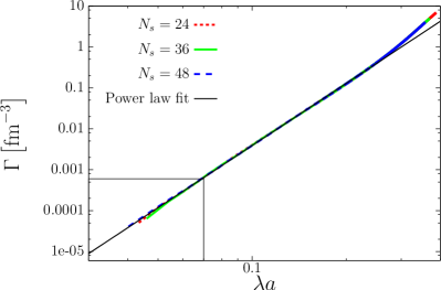
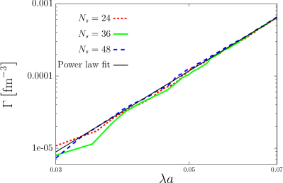
Figure 2: Left panel: The integrated spectral density normalized by the volume for the ensembles listed in Tab. 1. The continuous line corresponds to a power law fit to the data on the largest volume ($N_{s}=48$) in the interval $\left[0.09,0.12\right]$. Right panel: Zoom in the spectral region around $\lambda\simeq 0$ i.e. around the “spectrum edge”.

The combination of localization and small spectral density leads one to expect that the low-lying eigenmodes are not mixed by the fluctuations of the gauge field. As a consequence, the corresponding eigenvalues are expected to be uncorrelated, thus following Poisson statistics. Notice that low spectral density alone does not necessarily lead to uncorrelated eigenvalues: this is the case in the two-flavor Schwinger model [9]. Moving towards the bulk of the spectrum, the density of eigenvalues increases rapidly, and the eigenvectors start to become delocalized. The typical gauge field fluctuations are then expected to easily mix the eigenmodes, as their energy difference is small and they also have significant spatial overlap. In this case, the corresponding eigenvalues are expected to follow the Wigner-Dyson statistics of the appropriate ensemble of RMT, which is the unitary ensemble in the case of QCD.

To detect the expected transition in the spectral statistics we use the distribution of spacings between neighboring eigenvalues on the scale of the local average level spacing, the so-called unfolded level spacing distribution (ULSD). For Poisson statistics the ULSD is a simple exponential, while for Wigner-Dyson statistics it is well approximated by the so-called Wigner surmise for the appropriate random matrix ensemble. We display our results in Fig. 3. For comparison we include the exponential (dotted line) and the unitary Wigner surmise (continuous line) in each panel. In panel $a$ we see a nice agreement with the exponential, indicating that the low modes follow Poisson statistics. In panel $b$ we show the ULSD in a spectral window where the spectral density is one order of magnitude larger. There is a clear signal of a deviation from the Poisson exponential towards the unitary Wigner surmise, which increases as one moves further up along the spectrum (panel $c$). Approaching even more the bulk of the spectrum (panel $d$) the spectral statistics nearly agrees with the Wigner surmise. Thus the eigenvalue statistics in the bulk of the Dirac spectrum is well described by Random Matrix Theory in the high temperature quark-gluon-plasma phase as well as in the low temperature hadronic phase.

\psfrag{RMT}[b][b][0.65]{$~{}~{}RMT$}\psfrag{Poisson}[b][b][0.65]{$Poisson$}\psfrag{48}[b][b][0.65]{$~{}~{}~{}~{}~{}~{}~{}~{}~{}~{}~{}~{}~{}~{}~{}~{}~{}~{}~{}N_{s}=48$ data}\psfrag{a}[b][b][1]{$a:0.15\leq\lambda a\leq 0.19$}\psfrag{b}[b][b][1]{$b:0.31\leq\lambda a\leq 0.32$}\psfrag{c}[b][b][1]{$c:0.34\leq\lambda a\leq 0.35$}\psfrag{d}[b][b][1]{$d:0.36\leq\lambda a\leq 0.375$}\psfrag{yaxis}[b][b][0.7]{$p\left(\Delta\lambda\right)$}\psfrag{xaxis}[b][b][0.7]{$\Delta\lambda$}\includegraphics[width=130.08731pt,keepaspectratio]{Figs/0_15_0_19_484_pos.eps}

\psfrag{RMT}[b][b][0.65]{$~{}~{}RMT$}\psfrag{Poisson}[b][b][0.65]{$Poisson$}\psfrag{48}[b][b][0.65]{$~{}~{}~{}~{}~{}~{}~{}~{}~{}~{}~{}~{}~{}~{}~{}~{}~{}~{}~{}N_{s}=48$ data}\psfrag{a}[b][b][1]{$a:0.15\leq\lambda a\leq 0.19$}\psfrag{b}[b][b][1]{$b:0.31\leq\lambda a\leq 0.32$}\psfrag{c}[b][b][1]{$c:0.34\leq\lambda a\leq 0.35$}\psfrag{d}[b][b][1]{$d:0.36\leq\lambda a\leq 0.375$}\psfrag{yaxis}[b][b][0.7]{$p\left(\Delta\lambda\right)$}\psfrag{xaxis}[b][b][0.7]{$\Delta\lambda$}\includegraphics[width=130.08731pt,keepaspectratio]{Figs/0_31_0_32_484_pos.eps}

\psfrag{RMT}[b][b][0.65]{$~{}~{}RMT$}\psfrag{Poisson}[b][b][0.65]{$Poisson$}\psfrag{48}[b][b][0.65]{$~{}~{}~{}~{}~{}~{}~{}~{}~{}~{}~{}~{}~{}~{}~{}~{}~{}~{}~{}N_{s}=48$ data}\psfrag{a}[b][b][1]{$a:0.15\leq\lambda a\leq 0.19$}\psfrag{b}[b][b][1]{$b:0.31\leq\lambda a\leq 0.32$}\psfrag{c}[b][b][1]{$c:0.34\leq\lambda a\leq 0.35$}\psfrag{d}[b][b][1]{$d:0.36\leq\lambda a\leq 0.375$}\psfrag{yaxis}[b][b][0.7]{$p\left(\Delta\lambda\right)$}\psfrag{xaxis}[b][b][0.7]{$\Delta\lambda$}\includegraphics[width=130.08731pt,keepaspectratio]{Figs/0_34_0_35_484_pos.eps}

\psfrag{RMT}[b][b][0.65]{$~{}~{}RMT$}\psfrag{Poisson}[b][b][0.65]{$Poisson$}\psfrag{48}[b][b][0.65]{$~{}~{}~{}~{}~{}~{}~{}~{}~{}~{}~{}~{}~{}~{}~{}~{}~{}~{}~{}N_{s}=48$ data}\psfrag{a}[b][b][1]{$a:0.15\leq\lambda a\leq 0.19$}\psfrag{b}[b][b][1]{$b:0.31\leq\lambda a\leq 0.32$}\psfrag{c}[b][b][1]{$c:0.34\leq\lambda a\leq 0.35$}\psfrag{d}[b][b][1]{$d:0.36\leq\lambda a\leq 0.375$}\psfrag{yaxis}[b][b][0.7]{$p\left(\Delta\lambda\right)$}\psfrag{xaxis}[b][b][0.7]{$\Delta\lambda$}\includegraphics[width=130.08731pt,keepaspectratio]{Figs/0_36_03735_484_pos.eps}

Figure 3: The unfolded level spacing ($\Delta\lambda=\frac{\lambda_{n+1}-\lambda_{n}}{\langle\lambda_{n+1}-\lambda_{n}\rangle}$) distribution (ULSD) in four non-overlapping spectral windows. The dashed and dotted line indicates the ULSD for Poisson statistics and for RMT statistics respectively. The spatial extension of the lattice is $N_{s}=48$ and the temperature is $T=394$ MeV.

It is instructive to check the volume dependence of the transition in the spectrum. Instead of comparing the whole distribution in a given spectral window on different volumes, it is simpler to just pick one parameter of the distribution and see how it changes along the spectrum. For this purpose we use the variance of the ULSD, which can be computed analytically for both kinds of statistics. We show our results in Fig. 4. It is clearly seen that the transition becomes sharper for larger volumes, which suggests that it becomes a true phase transition in the thermodynamic limit. A proper finite size scaling analysis of the transition and a comparison with the Anderson transition is discussed in [10]. In a finite volume the separation between localized and delocalized modes is not sharp, and so the definition of the “mobility edge” $\lambda_{c}$ is not unique. Here we define it to be the inflection point of the variance of the ULSD. If there is a genuine phase transition, this point should tend to the true critical point in the thermodynamic limit. The critical statistics is examined in [11].

\psfrag{yaxis}[b][b][0.8]{$\sigma^{2}\left(\lambda a\right)$}\psfrag{xaxis}[b][b][0.8]{$\lambda a$}\psfrag{24}[b][b][0.8]{$~{}~{}~{}~{}~{}~{}N_{s}=24$}\psfrag{36}[b][b][0.8]{$~{}~{}~{}~{}~{}~{}N_{s}=36$}\psfrag{48}[b][b][0.8]{$~{}~{}~{}~{}~{}~{}N_{s}=48$}\psfrag{Poisson}[b][b][0.8]{Poisson}\psfrag{RMT}[b][b][0.8]{~{}RMT}\includegraphics[width=203.80193pt,clip={true}]{Figs/ulsd_var_dynamical_conv_pos.eps}

Figure 4: The variance of the local ULSD for three different volumes. The smooth and the dashed line indicates the variance of ULSD in the case of Poisson statistics and RMT statistics respectively.

As long as hadronic correlators are concerned, the “mobility edge” $\lambda_{c}$ acts as an effective gap in the spectrum. To see this explicitly, let us write the quark propagator in terms of the Dirac eigenmodes

$$G\left(x,y\right)=\sum_{n}\frac{1}{i\lambda_{n}+m_{q}}\psi_{n}\left(x\right)\psi^{\dagger}_{n}\left(y\right),$$ (1)

where $x,y$ are space time points, $m_{q}$ is the bare quark mass and the sum is over all eigenmodes $\psi_{n}$ of the Dirac operator. Firstly, the sum in (1) is dominated by the low eigenmodes, which are localized. On the other hand, for a localized mode, the product $\psi\left(x\right)\psi^{\dagger}\left(y\right)$ is practically zero when the distance between $x$ and $y$ is larger than the localization length, and so localized modes do not propagate quarks to large distances. Therefore, long range hadronic correlators receive contributions only from the delocalized eigenmodes, for which $\lambda>\lambda_{c}$.

A possible definition of the localisation length $l$ of localized modes is just $l=a(V\cdot PR)^{\frac{1}{4}}=a\left(\sum_{x}|\psi^{\dagger}\left(x\right)\psi\left(x\right)|^{2}\right)^{-\frac{1}{4}}$. In Fig. 5 we show $l$ in units of the inverse temperature for three different lattice spacings. The localization length in units of the inverse temperature remains around unity for each lattice spacing. This suggests that the length scale of the localized modes is set by the inverse temperature. The low localized eigenmodes are squeezed in the spatial directions in the same way as in the temporal direction.

\psfrag{yaxis}[b][b][1]{$\langle PR\rangle=\langle\frac{1}{V}\left(\sum_{x}|\psi_{i}\left(x\right)\psi_{i}^{\dagger}\left(x\right)|^{2}\right)^{-1}\rangle$}\psfrag{xaxis}[b][b][1]{$a\lambda$}\psfrag{24}[b][b][1.25]{$~{}~{}~{}~{}~{}~{}N_{s}=24$}\psfrag{36}[b][b][1.25]{$~{}~{}~{}~{}~{}~{}N_{s}=36$}\psfrag{48}[b][b][1.25]{$~{}~{}~{}~{}~{}~{}N_{s}=48$}\psfrag{Poisson}[b][b][1.25]{Poisson}\psfrag{RMT}[b][b][1.25]{RMT}\includegraphics[width=203.80193pt,clip={true}]{Figs/lvsT.eps}

Figure 5: The temperature dependence of the localization length in units of the inverse temperature for three different lattice spacings.

The “mobility edge” behaves as it were effectively a gap in the spectrum with respect to the long range correlators. To determine how this effective gap depends on the temperature we define a rescaled “mobility edge” $\lambda^{rs}_{c}\equiv\frac{\lambda_{c}}{m_{ud}}$, where $m_{ud}$ is the bare quark mass. This quantity has a well defined continuum limit [7]. We show our results for the rescaled “mobility edge” in Fig. 6 as a function of the temperature for three different lattice spacings. The points fall nearly on a straight line. The systematic error arising from finite lattice spacing effects are comparable to our statistical errors. To determine the possible deviations from the linear behavior of $\lambda^{rs}_{c}$ we make a second order polynomial fit ($\chi^{2}=1.32$). The coefficient of the first order term in $\frac{T-T_{c}}{T_{c}}$ is two orders of magnitude larger than the coefficient of the second order term, so to a good approximation $\lambda^{rs}_{c}$ increases linearly with the temperature. Notice that the “mobility edge” is already two orders of magnitude larger than the quark mass just above $T_{c}$. We get a good crosscheck for our results by extrapolating this fit to $\lambda^{rs}_{c}$ equal to zero, which corresponds to the temperature at which the localized modes start to appear. We find for this point T$\simeq$170 MeV, which is above the point where the finite temperature chiral crossover takes place [12, 13], consistently with the absence of localised modes at low temperature.

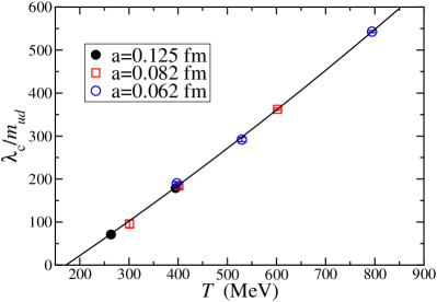
Figure 6: The rescaled “mobility edge” $\lambda^{rs}_{c}=\frac{\lambda_{c}}{m_{ud}}$ as a function of the temperature for three different lattice spacings.

4 Conclusion

We have shown that even at temperatures well above $T_{c}$ the Dirac operator seems to have no spectral gap. However, the low-lying modes behave quite differently compared to the modes in the bulk: they are localized on the scale of the inverse temperature, and the corresponding eigenvalues are statistically independent. Above the “mobility edge”, the eigenmodes are delocalized, as in the low temperature regime. This “mobility edge” plays the role of an effective gap with respect to the long range correlators. Here long range means that the separation of the fields in the correlator is larger than the inverse temperature.

References

- [1] T. Banks and A. Casher, Nucl. Phys. B 169, 103 (1980).
- [2] E. V. Shuryak and J. J. M. Verbaarschot, Nucl. Phys. A 560, 306 (1993) [hep-th/9212088].
- [3] M. E. Berbenni-Bitsch, S. Meyer, A. Schäfer, J. J. M. Verbaarschot and T. Wettig, Phys. Rev. Lett. 80, 1146 (1998) [hep-lat/9704018].
- [4] A. M. García-García and J. C. Osborn, Nucl. Phys. A 770, 141 (2006) [hep-lat/0512025].
- [5] T. G. Kovács, Phys. Rev. Lett. 104, 031601 (2010) [arXiv:0906.5373 [hep-lat]].
- [6] T. G. Kovács and F. Pittler, Phys. Rev. Lett. 105, 192001 (2010) [arXiv:1006.1205 [hep-lat]].
- [7] T. G. Kovács and F. Pittler, Phys. Rev. D 86, 114515 (2012) [arXiv:1208.3475 [hep-lat]].
- [8] Y. Aoki, Z. Fodor, S. D. Katz, K. K. Szabó, Phys. Lett. B643 46 (2006) [hep-lat/0609068].
- [9] W. Bietenholz, I. Híp and D. Landa-Marbán, arXiv:1310.3427 [hep-lat].
- [10] M. Giordano, T. G. Kovács and F. Pittler, PoS LATTICE 2013 213 (2013).
- [11] S.M. Nishigaki, PoS LATTICE 2013 018 (2013).
- [12] S. Borsányi et al. [Wuppertal-Budapest Collaboration], JHEP 1009, 073 (2010) [arXiv:1005.3508 [hep-lat]].
- [13] A. Bazavov, T. Bhattacharya, M. Cheng, C. DeTar, H. T. Ding, S. Gottlieb, R. Gupta and P. Hegde et al., Phys. Rev. D 85, 054503 (2012) [arXiv:1111.1710 [hep-lat]].