An Inexact Proximal Path-Following Algorithm
for Constrained Convex Minimization

Abstract

Many scientific and engineering applications feature nonsmooth convex minimization problems over convex sets. In this paper, we address an important instance of this broad class where we assume that the nonsmooth objective is equipped with a tractable proximity operator and that the convex constraint set affords a self-concordant barrier. We provide a new joint treatment of proximal and self-concordant barrier concepts and illustrate that such problems can be efficiently solved, without the need of lifting the problem dimensions, as in disciplined convex optimization approach. We propose an inexact path-following algorithmic framework and theoretically characterize the worst-case analytical complexity of this framework when the proximal subproblems are solved inexactly. To show the merits of our framework, we apply its instances to both synthetic and real-world applications, where it shows advantages over standard interior point methods. As a by-product, we describe how our framework can obtain points on the Pareto frontier of regularized problems with self-concordant objectives in a tuning free fashion.

1 Problem statement and motivation

We consider the following constrained convex minimization problem, which has aplenty applications in diverse disciplines, including machine learning, signal processing, statistics, and control [13, 22, 23, 43]:

(1) $$g^{*}:=\min_{\mathbf{x}\in\Omega}g(\mathbf{x}).$$

Here, $\Omega\subseteq\mathbb{R}^{n}$ is a nonempty, closed and convex set and $g$ is a (possibly) non-smooth convex function from $\mathbb{R}^{n}\to\mathbb{R}\cup\left\{+\infty\right\}$.

Problem (1) is sufficiently generic to cover many optimization settings considered in the literature. Under mild assumptions on $g$ and $\Omega$, general convex optimization methods such as mirror descent, projected subgradient as well as Frank-Wolfe methods can be applied to solve (1), as long as the projection on $\Omega$ can be computed efficiently [1, 6, 9, 33]. Theoretically, such methods are usually slowly convergent (e.g., $O(1/\sqrt{k})$ global convergence rate, where $k$ is the iteration counter) and sensitive to the choice of step-sizes [31], which constitutes them impractical for many applications.

In the case $\Omega$ has an explicit form, e.g., $\Omega:=\left\{\mathbf{x}\in\mathbb{R}^{n}~{}|~{}c_{i}(\mathbf{x})\leq 0,~{}i=1,\cdots,m\right\}$, where $c_{i}(\cdot)$ are generic convex functions for $i=1,\cdots,m$, nonsmooth optimization methods such as level and bundle methods are also potential candidates to solve (1) [12, 25, 28, 31, 41]. Though, similarly to subgradient methods, bundle schemes also have slow global convergence rate (e.g., $\mathcal{O}(1/\sqrt{k})$) when applying to nonsmooth problems, except for the cases where particular assumptions are made [27, 31].

When $g$ is a smooth term and projections on $\Omega$ are expensive to compute, sequential convex programming approach such as sequential quadratic programming (SQP) constitutes an efficient strategy for solving (1), see, e.g., [1, 18, 37]. However, this approach is usually generic and still requires a globalization strategy to ensure convergence. Along this line, the most famous class of algorithms is that of interior point methods (IPM) that solve standard conic programming problems in polynomial time [10, 34]. The key structure exploited in conventional IPMs is the existence of a barrier function for the feasible set $\Omega$ (cf., Section 2).

In such cases, one considers the penalized family of parametric composite convex optimization problems:

(2) $$\min_{\mathbf{x}\in\mathbf{R}^{n}}\left\{F(\mathbf{x};t):=f(\mathbf{x})+t^{-1}g(\mathbf{x})\right\},$$

where $t>0$ is a penalty parameter and $f$ is the barrier function over the set $\Omega$. By solving (2) for a sequence of decreasing $t$ values, i.e., $t\downarrow 0^{+}$, we can trace the analytic central path $\mathbf{x}^{*}_{t}$ of (2) as it converges to the solution $\mathbf{x}^{\ast}$ of (1).

However, assuming no further structure in $f$, the resulting path-following scheme is not guaranteed to converge, and solving (2) becomes harder as $t\downarrow 0^{+}$; see, e.g., [30]. Aptly, Nesterov and Nemirovskii [31] introduced the self-concordance concept (cf., Section 2 for definitions), which characterizes a broad collection of penalty functions $f$ and guarantees the polynomial-solvability of (2), by sequentially using Newton methods.

Within the IPM context, $g$ is usually assumed to be a smooth term. When $g$ is a nonsmooth term, it has a direct impact on the computational effort. Such problems do occur frequently in applications. Examples include but are not limited to sparse concentration matrix estimation with $\ell_{1}$-norm (eq. (11) in [38]), data clustering with $\ell_{1}$-norm (semidefinite programming reformulation in Section 4.1 of [24]), spectral line estimation with atomic norms (eq. (2.6) in [45] and eq. (3.4) in [11]), etc. Since off-the-shelf IPMs usually approximate $g^{\ast}$ by solving a sequence of smooth problems [30, 31], $g$ in (2) must allow a reformulation where standard IP solvers can be applied (i.e., via disciplined convex optimization (DCO) techniques [19]).

Nevertheless, the DCO approach can inflate the problem dimensions, and often suffers from the curse-of-dimensionality. As a concrete example, consider the max-norm clustering problem [24], where we seek a clustering matrix $\mathbf{K}$ that minimizes disagreement with a given affinity matrix $\mathbf{A}$:

(3) $$\begin{array}[]{cl}\displaystyle\min_{\mathbf{L},\mathbf{R},\mathbf{K}\in\mathbb{R}^{p\times p}}&\left\|\mathrm{vec}\left(\mathbf{K}-\mathbf{A}\right)\right\|_{1}\\ \textrm{s.t.}&\begin{bmatrix}\mathbf{L}&\mathbf{K}\\ \mathbf{K}^{T}&\mathbf{R}\end{bmatrix}\succeq 0,~{}\mathbf{L}_{ii}\leq 1,~{}\mathbf{R}_{ii}\leq 1,~{}i=1,\dots,p,\end{array}$$

where $\mathrm{vec}$ is the vectorization operator of a matrix (i.e., $\mathrm{vec}(\mathbf{X}):=(\mathbf{X}_{1}^{T},\cdots,\mathbf{X}_{n}^{T})^{T}$, where $\mathbf{X}_{i}$ is the $i$-th column of $\mathbf{X}$). This non-smooth formulation affords rigorous theoretical guarantees for its solution quality and can be formulated as a standard conic program. Unfortunately, we need to add $\mathcal{O}(p^{2})$ slack variables to process the $\ell_{1}$-norm term and the linear constraints. Moreover, the scaling factors (e.g., the Nesterov-Todd scaling factor regarding the semidefinite cone [35]) can create memory bottlenecks by destroying the sparsity of the underlying problem (e.g., by leading to dense KKT matrices in Newton systems).

1.1 Our approach

In general, when the penalty function $f$ has a Lipschitz continuous gradient [31] and $g$ has a computable proximity operator (cf., Section 2 for definitions), several efficient convex optimization algorithms for solving (2) exist [5, 7, 31, 32]. However, to the best of our knowledge, there has been no unified framework for path-following schemes of (2) where $f$ is a self-concordant barrier (hence, non-globally Lipschitz continuous gradient) and $g$ is a non-smooth term with proximal tractability (i.e., the proximal operator of $g$ is efficient to compute).

To this end, we address (1) with a new proximal path-following scheme, which solves (2) for a sequence of adaptively selected parameters $t_{k}$. Our scheme guarantees the following: If $\mathbf{x}_{t_{k}}$ is an approximation of $\mathbf{x}^{*}_{t_{k}}$ of (1), by solving instances of (2) for $t=t_{k}$—i.e., within some user-defined accuracy, then our method produces an approximate solution $\mathbf{x}_{t_{k+1}}$ of $\mathbf{x}^{*}_{t_{k+1}}$ of (1) for $t=t_{k+1}$ within the same accuracy by performing only one inexact proximal-Newton (PN) step. Moreover, our scheme adaptively updates the regularization parameter to trace the path of solutions, towards the optimal solution of (1).

But, how such a scheme is advantageous in practice? First, due to the non-smoothness of the objective function, solving (2) can be a strenuous task. However, using proximal-Newton/gradient strategies to solve approximations of (2) has been a major research area over the last decade, broadly known as composite optimization, where many accurate and scalable algorithms are customized for different $g$ functions [7, 8, 32]. These methods are theoretically as fast as the advanced “Hessian-free” IPM techniques, which use conjugate gradients, since $\nabla^{2}f(\mathbf{x})\succ 0$ for self concordant-barriers. Our path following scheme leverages such algorithms as a black-box to solve (1): as we handle the non-smooth term $g$ directly with proximity operators, we retain the original problem structure (i.e., we do not inflate problem dimensions or add additional constraints by lifting the nonsmooth term via slack variables).

Second, adaptively updating the regularization parameter in composite optimization problems has itself attracted a great deal of interest; cf., the class of homotopy and continuation methods [21]. Many of these approaches lose their theoretical guarantees (if any) when the composite minimization problem has a self-concordant smooth term instead of a Lipschitz continuous gradient smooth term. Our scheme provides a rigorous way of updating the regularizer weights and can be easily adapted for applications with self-concordant data terms [22, 38, 43], where none of these methods apply.

Our contributions: Our specific contributions in this paper are as follows:

• We extend the notion of path-following scheme to handle composite forms in order to approximately track the solution trajectory of (2). As a consequence, we obtain an approximate solution of (1) by controlling the parameter $t$ to $0^{+}$.

• We provide an explicit formula to adaptively update the parameter $t$ with convergence guarantees, without any manual tuning strategy.

• We provide a theoretical analysis of the worst-case analytical complexity of our scheme to obtain a sequence of approximate solutions, as $t$ varies, while allows one to inexactly compute the proximal-Newton directions up to a given accuracy. The worst-case analytical complexity of our method remains the same order as in conventional path-following interior point methods [31].

Paper outline. Section 2 recalls the definitions of self-concordant functions and barriers and sets up optimization preliminaries. Section 3 deals with the inexact proximal-Newton iteration scheme for solving (2) at a fixed value of the parameter $t$. Section 4 presents the path-following framework with inexact proximal-Newton iterations and analyzes its convergence and worst-case analytical complexity. Section 5 specifies our framework to solve constrained convex minimization problems of the form (1). Section 6 presents numerical experiments that highlight the strengths and weaknesses of our framework. Technical proofs are given in the appendix.

2 Preliminaries

In this section, we set up the necessary notation, definitions and basic properties related to problem (2).

2.1 Basic definitions

Given $\mathbf{x},\mathbf{y}\in\mathbb{R}^{n}$, we use $\mathbf{x}^{T}\mathbf{y}$ to denote the inner product in $\mathbb{R}^{n}$. For a proper, lower semicontinuous convex function $f$, we denote its domain by $\mathrm{dom}\left(f\right)$ (i.e., $\mathrm{dom}\left(f\right):=\left\{\mathbf{x}\in\mathbb{R}^{n}~{}|~{}f(\mathbf{x})<+\infty\right\}$ and its subdifferential at $\mathbf{x}$ by $\partial{f}(\mathbf{x}):=\left\{\mathbf{v}\in\mathbb{R}^{n}~{}|~{}f(\mathbf{y})\geq f(\mathbf{x})+\mathbf{v}^{T}(\mathbf{y}-\mathbf{x}),~{}\forall\mathbf{y}\in\mathrm{dom}\left(f\right)\right\}$. We also define $\mathrm{Dom}(f):=\mathrm{cl}(\mathrm{dom}\left(f\right))$ the closure of $\mathrm{dom}\left(f\right)$ [39].

For a given twice differentiable function $f$ such that $\nabla^{2}f(\mathbf{x})\succ 0$ at $\mathbf{x}\in\mathrm{dom}\left(f\right)$, we define the local norm $\left\|\mathbf{u}\right\|_{\mathbf{x}}:=[\mathbf{u}^{T}\nabla^{2}f(\mathbf{x})\mathbf{u}]^{1/2}$ for any $\mathbf{u}\in\mathbb{R}^{n}$ while the dual norm is given by $\left\|\mathbf{v}\right\|_{\mathbf{x}}^{*}:=\max_{\left\|\mathbf{u}\right\|_{\mathbf{x}}\leq 1}\mathbf{u}^{T}\mathbf{v}=[\mathbf{v}^{T}\nabla^{2}f(\mathbf{x})^{-1}\mathbf{v}]^{1/2}$ for any $\mathbf{v}\in\mathbb{R}^{n}$. It is clear that the Cauchy-Schwarz inequality holds, i.e., $\mathbf{u}^{T}\mathbf{v}\leq\left\|\mathbf{u}\right\|_{\mathbf{x}}\left\|\mathbf{v}\right\|^{*}_{\mathbf{x}}$. For our analysis, we also use two simple convex functions $\omega(t):=t-\ln(1+t)$ for $t\geq 0$ and $\omega_{*}(t):=-t-\ln(1-t)$ for $t\in[0,1)$, which are strictly increasing in their domain.

An important concept in this paper is the self-concordance property [31, 34].

Definition 1.

A convex function $\varphi:\mathrm{dom}\left(\varphi\right)\subseteq\mathbb{R}\rightarrow\mathbb{R}$ is called standard self-concordant if $\left|\varphi^{\prime\prime\prime}(\tau)\right|\leq 2\varphi^{\prime\prime}(\tau)^{3/2}$ for all $\tau\in\mathrm{dom}\left(\varphi\right)$. A function $f:\mathrm{dom}\left(f\right)\subseteq\mathbb{R}^{n}\rightarrow\mathbb{R}$ is self-concordant if $\mathbf{x}\in\mathrm{dom}\left(f\right)$ and $\mathbf{v}\in\mathbb{R}^{n}$ such that $\mathbf{x}+\tau\mathbf{v}\in\mathrm{dom}\left(f\right)$, the function $\varphi(\tau):=f(\mathbf{x}+\tau\mathbf{v})$ is standard self-concordant .

Definition 2.

A standard self-concordant function $f:\mathrm{dom}\left(f\right)\to\mathbb{R}$ is a $\nu$-self-concordant barrier for the set $\mathrm{Dom}(f)$ with parameter $\nu>0$, if

$$\sup_{\mathbf{u}\in\mathbb{R}^{n}}\left\{2\nabla{f}(\mathbf{x})^{T}\mathbf{u}-\|\mathbf{u}\|_{\mathbf{x}}^{2}\right\}\leq\nu,~{}~{}\forall\mathbf{x}\in\mathrm{dom}\left(f\right).$$

We note that when $\nabla^{2}f$ is non-degenerate (particularly, $\mathrm{dom}\left(f\right)$ contains no straight line [31, Theorem 4.1.3.]), a $\nu$-self-concordant function $f$ satisfies

(4) $${}\left\|\nabla f(\mathbf{x})\right\|_{\mathbf{x}}^{\ast}\leq\sqrt{\nu},~{}~{}\forall\mathbf{x}\in\mathrm{dom}\left(f\right).$$

For more details on self-concordant functions and self-concordant barriers, we refer the reader to Chapter 4 of [31]. Several simple sets are equipped with a self-concordant barrier. For instance, $f_{\mathbb{R}^{n}_{+}}(\mathbf{x}):=-\sum_{i=1}^{n}\log(x_{i})$ is an $n$-self-concordant barrier of the orthogonal cone $\mathbb{R}^{n}_{+}$, $f(\mathbf{x},t)=-\log(t^{2}-\left\|\mathbf{x}\right\|_{2}^{2})$ is a $2$-self-concordant barrier of the Lorentz cone $\mathcal{L}_{n+1}:=\left\{(\mathbf{x},t)\in\mathbb{R}^{n}\times\mathbb{R}_{+}~{}|~{}\left\|\mathbf{x}\right\|_{2}\leq t\right\}$, and the semidefinite cone $\mathcal{S}^{n}_{+}$ is endowed with an $n$-self-concordant barrier $f_{\mathcal{S}_{+}^{n}}(\mathbf{X}):=-\log\det(\mathbf{X})$.

Given these definitions, we are now ready to state our main assumption used throughout this paper.

Assumption A. 1.

The function $f$ in (2) is a $\nu$-self-concordant barrier with $\nu>0$ for $\mathrm{Dom}(f)$. The function $g:\mathbb{R}^{n}\to\mathbb{R}\cup\left\{+\infty\right\}$ is proper, lower semi-continuous and convex.

2.2 Optimality condition of (2)

Given $t>0$, we assume that problem (2) has a solution $\mathbf{x}^{*}_{t}$. Since $f$ is strictly convex, this solution is also unique. The optimality condition of (2) can be written as

(5) $$\mathbf{0}\in\nabla{f}(\mathbf{x}^{*}_{t})+t^{-1}\partial{g}(\mathbf{x}^{*}_{t}).$$

The formula (5) expresses a monotone inclusion [16]. If $g$ is smooth, (5) reduces to $\nabla{f}(\mathbf{x}^{*}_{t})+t^{-1}\nabla{g}(\mathbf{x}^{*}_{t})=\mathbf{0}$, a system of nonlinear equations. Any $\mathbf{x}^{*}_{t}$ satisfying (5) is called a stationary point of (2), which is also a global optimum of (2), for given $t>0$. Let $\mathrm{dom}\left(F\right)\equiv\mathrm{dom}\left(F(\cdot;t)\right):=\mathrm{dom}\left(f\right)\cap\mathrm{dom}\left(g\right)$ for fixed $t>0$. Then $\mathbf{x}^{*}_{t}\in\mathrm{dom}\left(F\right)$.

Definition 3.

Let $\mathbf{x}\in\mathrm{dom}\left(f\right)$ such that $\nabla^{2}{f}(\mathbf{x})\succ 0$ and let $\mathbf{s}\in\mathbb{R}^{n}$ be an arbitrary given point. We define the operator $P^{g}_{\mathbf{x}}(\cdot;t)$ with an input $\mathbf{s}$ and a parameter $t>0$ as follows:

(6) $$P^{g}_{\mathbf{x}}(\mathbf{s};t)=\mathrm{arg}\!\!\min_{\mathbf{y}\in\mathbb{R}^{n}}\left\{t^{-1}g(\mathbf{y})+\frac{1}{2}\mathbf{y}^{T}\nabla^{2}f(\mathbf{x})\mathbf{y}-\mathbf{s}^{T}\mathbf{y}\right\}.$$

Since $\nabla^{2}{f}(\mathbf{x})\succ 0$, we can write (3) as

$$P^{g}_{\mathbf{x}}(\mathbf{s};t)=\mathrm{arg}\!\!\min_{\mathbf{y}\in\mathbb{R}^{n}}\left\{g(\mathbf{y})+\frac{t}{2}\left\|\mathbf{y}-\nabla^{2}f(\mathbf{x})^{-1}\mathbf{s}\right\|_{\mathbf{x}}^{2}\right\},$$

which requires to compute the proximal operator of $g$ at $\nabla^{2}f(\mathbf{x})^{-1}\mathbf{s}$ w.r.t. the weighted norm $\left\|\cdot\right\|_{\mathbf{x}}$. Given $\mathbf{x}$ and $\mathbf{s}$ as defined above, we define the following mapping:

(7) $$S_{\mathbf{x}}(\mathbf{s}):=\nabla^{2}{f}(\mathbf{x})\mathbf{s}-\nabla{f}(\mathbf{s}).$$

The optimality condition in (5) implies the following fixed-point characterization of the mapping $P^{g}_{\mathbf{x}}(\cdot;t)$. The proof can be found in [46].

Lemma 4.

Let $t>0$ be fixed. Then, the mapping $P_{\mathbf{x}}^{g}(\cdot;t)$ defined in (6) is co-coercive and therefore nonexpansive w.r.t. the local norms, i.e.:

(8) $$\mathrm{[co\textrm{-}coercive]:}~{}~{}~{}~{}~{} \left(P^{g}_{\mathbf{x}}(\mathbf{u};t)-P^{g}_{\mathbf{x}}(\mathbf{v};t)\right)^{T}(\mathbf{u}-\mathbf{v})\geq\left\|P^{g}_{\mathbf{x}}(\mathbf{u};t)-P^{g}_{\mathbf{x}}(\mathbf{v};t)\right\|_{\mathbf{x}}^{2},$$

(9) $$\mathrm{[nonexpansive]:}~{}~{} \left\|P^{g}_{\mathbf{x}}(\mathbf{u};t)-P^{g}_{\mathbf{x}}(\mathbf{v};t)\right\|_{\mathbf{x}}\leq\left\|\mathbf{u}-\mathbf{v}\right\|_{\mathbf{x}}^{*},~{}\forall\mathbf{u},\mathbf{v}\in\mathbb{R}^{n}.$$

Furthermore, the following fixed-point characterization holds:

(10) $$\mathbf{x}^{*}_{t}=P^{g}_{\mathbf{x}^{*}_{t}}\left(S_{\mathbf{x}^{*}_{t}}(\mathbf{x}^{*}_{t});t\right),$$

where $\mathbf{x}^{\ast}_{t}\in\mathrm{dom}\left(F\right)$ is the minimizer of (2), i.e., $\mathbf{x}^{\ast}_{t}\in\mathrm{arg}\!\!\displaystyle\min_{\mathbf{x}\in\mathbb{R}^{n}}F(\mathbf{x};t)$.

For our convergence analysis, we also need the following result.

Lemma 5.

For fixed $t>0$, let $\mathbf{x}^{*}_{t}$ be the unique solution of (2). Then, for any $\mathbf{x}\in\mathrm{dom}\left(F\right)$, the following estimate holds:

(11) $$\omega\left(\left\|\mathbf{x}-\mathbf{x}^{*}_{t}\right\|_{\mathbf{x}^{*}_{t}}\right)\leq F(\mathbf{x};t)-F(\mathbf{x}^{*}_{t};t).$$

Proof.

By the self-concordance property of $f$ for any $\mathbf{x}\in\mathrm{dom}\left(F\right)$, the convexity of $g$ and (5) it follows that there exists $\mathbf{v}_{t}^{*}\in\partial{g}(\mathbf{x}^{*}_{t})$ such that

$$F(\mathbf{x};t)-F(\mathbf{x}^{*}_{t};t) =f(\mathbf{x})-f(\mathbf{x}^{*}_{t})+t^{-1}\left(g(\mathbf{x})-g(\mathbf{x}^{*}_{t})\right)$$

$$\geq\left(\nabla{f}(\mathbf{x}^{*}_{t})+t^{-1}\mathbf{v}_{t}^{*}\right)^{T}(\mathbf{x}-\mathbf{x}^{*}_{t})+\omega\left(\left\|\mathbf{x}-\mathbf{x}^{*}_{t}\right\|_{\mathbf{x}^{*}_{t}}\right),~{}~{}\mathbf{v}_{t}^{*}\in\partial{g}(\mathbf{x}^{*}_{t}),$$

$$\overset{\tiny\eqref{eq:optimality_for_ln_barrier}}{=}\omega\left(\left\|\mathbf{x}-\mathbf{x}^{*}_{t}\right\|_{\mathbf{x}^{*}_{t}}\right),$$

which is indeed (11). ∎

3 Proximal-Newton iterations for fixed $t$

Let us consider the unconstrained problem (2) for a given fixed parameter value $t>0$. Since $f$ is self-concordant, we can approximate it around $\mathbf{x}_{t}\in\mathrm{dom}\left(F\right)$ via the second order Taylor series expansion:

(12) $$Q(\mathbf{x};\mathbf{x}_{t}):=f(\mathbf{x}_{t})\!+\!\nabla f(\mathbf{x}_{t})^{T}(\mathbf{x}\!-\!\mathbf{x}_{t})\!+\!\frac{1}{2}(\mathbf{x}\!-\!\mathbf{x}_{t})^{T}\nabla^{2}f(\mathbf{x}_{t})(\mathbf{x}\!-\!\mathbf{x}_{t}).$$

Given this quadratic surrogate of $f$, we can approximate $F(\mathbf{x};t)$ around $\mathbf{x}_{t}$ as:

(13) $$\widehat{F}(\mathbf{x};t,\mathbf{x}_{t}):=Q(\mathbf{x};\mathbf{x}_{t})+t^{-1}g(\mathbf{x}).$$

Starting from an arbitrary initial point $\mathbf{x}^{0}_{t}\in\mathrm{dom}\left(F\right)$ and given a fixed value $t>0$, the inexact full-step proximal-Newton method for solving (2) generates a sequence of points, by approximately minimizing the composite quadratic model (13) as

(16) $$\left\{\begin{array}[]{ll}\mathbf{x}^{+}_{t}\approx\operatorname*{arg\,min}_{\mathbf{x}\in\mathrm{dom}\left(F\right)}\widehat{F}(\mathbf{x};t,\mathbf{x}_{t}).\\ \mathbf{x}_{t}\leftarrow\mathbf{x}^{+}_{t}\end{array}\right.$$

Here, the “approximation” sense ($\approx$) highlights the inability of numerical methods to iteratively solve (16) with exact accuracy and $\leftarrow$ indicates the assignment operator.

Assume that $\nabla^{2}f(\mathbf{x}_{t})\succ 0$, then the minimization problem in (16) is a strongly convex program and it has the unique exact solution $\bar{\mathbf{x}}^{+}_{t}$, i.e.,

$$\left\{\begin{array}[]{ll}\bar{\mathbf{x}}^{+}_{t}:=\operatorname*{arg\,min}_{\mathbf{x}\in\mathrm{dom}\left(F\right)}\widehat{F}(\mathbf{x};t,\mathbf{x}_{t}).\\ \mathbf{x}_{t}\leftarrow\bar{\mathbf{x}}^{+}_{t}\end{array}\right.$$

Moreover, the following optimality condition holds

(17) $$\mathbf{0}\in\nabla{f}(\mathbf{x}_{t})+\nabla^{2}f(\mathbf{x}_{t})(\bar{\mathbf{x}}^{+}_{t}-\mathbf{x}_{t})+t^{-1}\partial{g}(\bar{\mathbf{x}}^{+}_{t}).$$

Due to (5), it is obvious to show that, if $\bar{\mathbf{x}}^{+}_{t}\equiv\mathbf{x}_{t}$, then $\mathbf{x}_{t}$ is the optimal solution of (2) for fixed $t$.

Remark 1.

In Phase I of Algorithm 1 below, we do not require $\nabla^{2}f(\mathbf{x})$ to be positive definite for all $\mathbf{x}\in\mathrm{dom}\left(F\right)$ as long as the subproblem (16) has solution. The positive definiteness of $\nabla^{2}f(\mathbf{x})$ is only needed in Phase II of this algorithm, where the path-following iterations take place.

The following table disambiguates the various notions introduced in this section:

Notation		Description
$\mathbf{x}_{t}^{*}$		Exact solution of (2) for fixed $t$.
$\bar{\mathbf{x}}_{t}^{+}$		Exact solution of (13) around $\mathbf{x}_{t}$ for fixed $t$.
$\mathbf{x}_{t}^{+}$		Inexact solution of (13) around $\mathbf{x}_{t}$ for fixed $t$.

3.1 Inexact solutions of (16)

In practice, computing $\bar{\mathbf{x}}_{t}^{+}$ is infeasible except for special cases. Thus, we can only solve (16) up to a given accuracy $\delta\geq 0$ using algorithmic solutions such as fast proximal-gradient methods and alternating direction methods of multipliers [7, 31, 32, 51] in the following sense.

Definition 6.

Given $t>0$ and a tolerance $\delta\geq 0$, a point $\mathbf{x}^{+}_{t}\in\mathrm{dom}\left(F\right)$ is called a $\delta$-solution to (16) if

(18) $$\widehat{F}(\mathbf{x}^{+}_{t};t,\mathbf{x}_{t})-\widehat{F}(\bar{\mathbf{x}}^{+}_{t};t,\mathbf{x}_{t})\leq\frac{\delta^{2}}{2}.$$

A useful inequality for our subsequent developments is given in the next lemma.

Lemma 7.

Given fixed $t>0$, the following inequality holds $\forall\mathbf{x}\in\mathrm{dom}\left(F\right)$:

(19) $$\frac{1}{2}\left\|\mathbf{x}-\bar{\mathbf{x}}^{+}_{t}\right\|_{\mathbf{x}_{t}}^{2}\leq\widehat{F}(\mathbf{x};t,\mathbf{x}_{t})-\widehat{F}(\bar{\mathbf{x}}^{+}_{t};t,\mathbf{x}_{t}),~{}~{}\forall\mathbf{x}\in\mathrm{dom}\left(F\right).$$

Proof.

Since $\nabla^{2}f(\mathbf{x}_{t})\succ 0$, the proof follows similar motions with the proof of Lemma 5, based on the optimality condition (17) and the convexity of $g$. ∎

This lemma, in combination with Definition 6, indicates that, if we can find a $\delta$-solution $\mathbf{x}^{+}_{t}$ using (16), then

(20) $$\left\|\mathbf{x}^{+}_{t}-\bar{\mathbf{x}}^{+}_{t}\right\|_{\mathbf{x}_{t}}\leq\delta.$$

3.2 Contraction property of inexact proximal-Newton iterations

In this subsection, we provide a theoretical characterization of the per-iteration behavior of the inexact full-step proximal-Newton scheme (16) for fixed $t>0$. Let $\mathbf{x}_{t}^{+}\in\mathrm{dom}\left(F\right)$ be a $\delta$-solution of (16) and let $\mathbf{x}^{*}_{t}$ be the exact solution of (2). We define

(21) $$\lambda_{t}:=\left\|\mathbf{x}_{t}-\mathbf{x}^{*}_{t}\right\|_{\mathbf{x}^{*}_{t}}\quad\text{and}\quad\lambda_{t}^{+}:=\left\|\mathbf{x}_{t}^{+}-\mathbf{x}^{*}_{t}\right\|_{\mathbf{x}^{*}_{t}},$$

as the weighted distance between $\mathbf{x}_{t}/\mathbf{x}^{*}_{t}$ and $\mathbf{x}_{t}^{+}/\mathbf{x}^{*}_{t}$, respectively. The following theorem characterizes the contraction properties of $\lambda_{t}$; the proof can be found in the appendix.

Theorem 8.

Given $\mathbf{x}_{t}\in\mathrm{dom}\left(F\right)$, let $\mathbf{x}^{+}_{t}$ be a $\delta$-solution of (16) for a given $\delta\geq 0$. Then, if $\lambda_{t}\in[0,1-\frac{\sqrt{2}}{2})$, we have

(22) $$\lambda^{+}_{t}\leq\frac{\delta}{1-\lambda_{t}}+\left(\frac{3-2\lambda_{t}}{1-4\lambda_{t}+2\lambda_{t}^{2}}\right)\lambda_{t}^{2}.$$

Moreover, the right-hand side of (22) is nondecreasing w.r.t. $\lambda_{t}$ and $\delta\geq 0$.

To illustrate the contraction properties of $\lambda_{t}$, we assume that the accuracy $\delta$ can be chosen such that $\delta:=\xi\lambda_{t}$ for a given $\xi\in(0,1)$. Furthermore, let us define $\varphi(\lambda,\xi):=\frac{\xi}{1-\lambda}+\frac{3\lambda-2\lambda^{2}}{1-4\lambda+2\lambda^{2}}$ on $[0,1-\frac{\sqrt{2}}{2})$. Then, (22) can be rewritten as

(23) $${}\lambda_{t}^{+}\leq\varphi(\lambda_{t},\xi)\lambda_{t}.$$

From (23), we observe that, if $\varphi(\lambda,\xi)\leq\omega<1$ for $\lambda\in[0,1-\sqrt{2}/2]$ and $\xi\in(0,1)$, the sequence of distances $\left\{\|\mathbf{x}^{+}_{t}-\mathbf{x}^{*}_{t}\|_{\mathbf{x}^{*}_{t}}\right\}_{+}$ by solving (16) becomes contractive, i.e., it ensures the convergence of the proximal-Newton scheme (16). To this end, we need to find a range of $\lambda_{t}$ values, (say $\Lambda$), such that $\varphi<1$. Varying $\xi$, we can choose this range $\Lambda$: Since $\varphi$ is non-decreasing, the larger $\xi$ is, the smaller the range of $\Lambda$ becomes. This observation is illustrated in Figure 1.

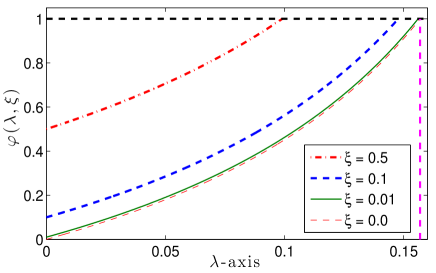
Fig. 1: The behavior of the contraction factor function $\varphi(\lambda,\xi)$ at different values of $\xi$.

For $\xi\in[0,0.5]$, the interval where $\varphi<1$ varies from $[0,0.098]$ to $[0,0.154]$. We observed also that, for $\xi=0.001$, the value of $\varphi$ is very close to the case of $\xi=0$. In practice, this suggests that if we set the accuracy $\delta<10^{-3}$, the inexact scheme performs closely to the ideal case (i.e., $\delta=0$).

Theoretically, if we assume that the subproblem (16) is solved exactly, then the estimate (22) reduces to $\bar{\lambda}_{t}^{+}\leq\left(\frac{3-2\bar{\lambda}_{t}}{1-4\bar{\lambda}_{t}+2\bar{\lambda}_{t}^{2}}\right)\bar{\lambda}_{t}^{2}$, where $\bar{\lambda}_{t}:=\left\|\bar{\mathbf{x}}_{t}-\mathbf{x}^{*}_{t}\right\|_{\mathbf{x}^{*}_{t}}$ and $\bar{\lambda}_{t}^{+}:=\left\|\bar{\mathbf{x}}_{t}^{+}-\mathbf{x}^{*}_{t}\right\|_{\mathbf{x}^{*}_{t}}$. The algorithms and the convergence theory corresponding to this case were studied in [46].

Now, within this section, we define $\mathbf{x}^{j}_{t}:=\mathbf{x}_{t}$, $\mathbf{x}^{j+1}_{t}:=\mathbf{x}^{+}_{t}$, $\lambda_{t}^{j}:=\lambda_{t}$, $\lambda_{t}^{j+1}:=\lambda_{t}^{+}$ and $\delta_{j}:=\delta$, where the index $j$ indicates the iteration counter for fixed $t$ starting from $j:=0$. An important consequence of Theorem 8 is the following corollary.

Corollary 9.

For a fixed $t>0$ and a given constant $c>0$, let $\{\mathbf{x}_{t}^{j}\}_{j\geq 0}$ be a sequence of $\delta_{j}$-solutions, generated by solving (16) approximately.

• If we choose $\delta_{j}$ and $\mathbf{x}^{0}_{t}$ such that $\delta_{j}\leq 0.15\lambda^{j}_{t}$ for $j\geq 0$ and $\lambda_{t}^{0}\leq 0.1427$, then the sequence of approximate solutions $\{\mathbf{x}^{j}_{t}\}_{j\geq 0}$ in (16) converges to $\mathbf{x}^{*}_{t}$ at a linear rate.

• If we choose $\delta_{j}$ and $\mathbf{x}^{0}_{t}$ such that $\delta_{j}\leq c\cdot(\lambda_{t}^{j})^{2}$ for $j\geq 0$ and

  $$\lambda_{t}^{0}\in\left[0,\min\left\{0.15,(1.177c+6.068)^{-1}\right\}\right],$$

  then the sequence of approximate solutions $\{\mathbf{x}^{j}_{t}\}_{j\geq 0}$ in (16) converges to $\mathbf{x}^{*}_{t}$ at a quadratic rate.

Proof.

$(a)$. For $\delta_{j}:=0.15\lambda^{j}_{t}$, we observe that $\varphi(\lambda,0.15)$ is increasing for $\lambda\in\Lambda:=[0,0.1427]$ and $\varphi(\lambda,0.15)<1$ for all $\lambda\in\Lambda$. Therefore, it follows from (22) that $\lambda_{t}^{j+1}\leq\max_{\lambda\in\Lambda}\left\{\varphi(\lambda,0.15)\right\}\cdot\lambda_{t}^{j}$ for $j\geq 0$, which implies the sequence $\left\{\lambda_{t}^{j}\right\}$ converges to zero at a linear rate. Since $\lambda_{t}^{j}:=\|\mathbf{x}^{j}_{t}-\mathbf{x}^{*}_{t}\|_{\mathbf{x}^{*}_{t}}$, the sequence $\{\mathbf{x}^{j}_{t}\}_{j\geq 0}$ also converges to $\mathbf{x}^{*}_{t}$ at a linear rate (in the weighted norm).

$(b)$.  For $\lambda_{t}^{j}\in[0,0.15]$, we can see that the weight factor of the second term in the right hand side of (22), i.e., $\frac{3-2\lambda_{t}^{j}}{1-4\lambda^{j}_{t}+2(\lambda_{t}^{j})^{2}}$, is increasing and moreover, $\frac{3-2\lambda_{t}^{j}}{1-4\lambda_{t}^{j}+2(\lambda^{j}_{t})^{2}}\leq 6.068$. Thus, for $\delta_{j}\leq c\cdot(\lambda_{t}^{j})^{2}$, we have

$$\lambda_{t}^{j+1}\leq\left(\frac{c}{1-\lambda_{t}^{j}}+6.068\right)(\lambda_{t}^{j})^{2}\leq\left(1.177c+6.068\right)(\lambda_{t}^{j})^{2}.$$

From this inequality, we can easily check that, if $\lambda_{t}^{0}\leq\min\left\{0.15,(1.177c+6.068)^{-1}\right\}$ then $\lambda_{t}^{j+1}\leq C\cdot(\lambda_{t}^{j})^{2}$ for $C:=1.177c+6.068$. This estimate shows that the sequence $\left\{\lambda_{t}^{j}\right\}_{j\geq 0}$ converges to zero at a quadratic rate. Consequently, the sequence $\{\mathbf{x}^{j}_{t}\}_{j\geq 0}$ also converges to $\mathbf{x}^{*}_{t}$ at a quadratic rate (in the weighted norm). ∎

4 A proximal path following framework

Our discussion so far focuses on the case of minimizing (16) for a fixed $t>0$. Nevertheless, in order to solve the initial problem (1), one requires to trace the sequence of solutions as $t_{k}\downarrow 0^{+}$. For smooth self-concordant barrier function minimization problems, Nesterov and Nemirovskii in [31, 34] presented a path following strategy where a single Newton step per iteration is used, for each well-chosen penalty parameter $t_{k}$. Here, we adopt a similar strategy to handle composite self-concordant barrier problems of the form (2) with a possibly nonsmooth convex function $g$, mutatis mutandis.

Our contribution lies at the adaptive selection of $t$: given an anchor point $\mathbf{x}_{t_{k}}$ obtained using $t_{k}>0$, we compute an approximate solution $\mathbf{x}_{t_{k+1}}$ as:

(24) $$\mathbf{x}_{t_{k\!+\!1}}\!:\approx\!\operatorname*{arg\,min}_{\mathbf{x}\in\mathrm{dom}\left(F\right)}\Big{\{} \nabla f(\mathbf{x}_{t_{k}})^{T}(\mathbf{x}\!-\!\mathbf{x}_{t_{k}})\!+\!\frac{1}{2}(\mathbf{x}\!-\!\mathbf{x}_{t_{k}})^{T}\nabla^{2}{f}(\mathbf{x}_{t_{k}})(\mathbf{x}\!-\!\mathbf{x}_{t_{k}})+t_{k+1}^{-1}g(\mathbf{x})\Big{\}},$$

where $t_{k+1}$ is adaptively updated per iteration, based on $t_{k}$; “$:\approx$” is defined as in Definition 6; and the index $k$ is to distinguish it from the index $j$ for fixed $t$. In stark contrast, classical path-following (homotopy or continuation) methods [17, 20] usually discretize the parameter $t$ a priori and then solve (2) over this grid.

Our proximal path following scheme goes through the following motions: Starting from an initial value $t=t_{0}$ and an anchor point $\mathbf{x}^{0}$, we solve (24) to obtain an approximate solution $\mathbf{x}_{t_{0}}$ to $\bar{\mathbf{x}}_{t_{0}}$, i.e., the exact solution of (16) at $t=t_{0}$. The initial selection of $t_{0}$ is generally problem dependent. Section 4.3 describes a procedure on how to compute a good starting point $\mathbf{x}_{t_{0}}$. Then, at the $k$-th iteration and given $\mathbf{x}_{t_{k}}$, the scheme uses $t_{k}$ to compute $t_{k+1}$ parameter and performs a single proximal-Newton (PN) iteration (i.e., solving (16) once for $t=t_{k+1}$) to approximately compute $\mathbf{x}_{t_{k+1}}$. Moreover, for each iteration, we provably show the proximity of $\mathbf{x}_{t_{k}}$ to $\mathbf{x}^{*}_{t_{k}}$. This strategy is illustrated in Figure 2.

Fig. 2: The approximate sequence $\{x_{t_{k}}\}_{k\geq 0}$ along the solution trajectory $x^{*}_{t_{k}}$.

4.1 Quadratic convergence region

Based on (21), we define $\lambda_{t_{k+1}}:=\|\mathbf{x}_{t_{k}}-\mathbf{x}^{*}_{t_{k+1}}\|_{\mathbf{x}^{*}_{t_{k+1}}}$ and $\lambda_{t_{k+1}}^{+}:=\|\mathbf{x}_{t_{k+1}}-\mathbf{x}^{*}_{t_{k+1}}\|_{\mathbf{x}^{*}_{t_{k+1}}}$. Given these definitions, for $t\equiv t_{k+1}$ and given the analysis in Section 3.2, (22) becomes

(25) $$\lambda_{t_{k+1}}^{+}\leq\frac{\delta_{k}}{1-\lambda_{t_{k+1}}}+\left(\frac{3-2\lambda_{t_{k+1}}}{1-4\lambda_{t_{k+1}}+2\lambda_{t_{k+1}}^{2}}\right)\lambda_{t_{k+1}}^{2},$$

provided that $0\leq\lambda_{t_{k+1}}<1-\sqrt{2}/2$. The index $k+1$ shows that we first update the parameter $t$ from $t_{k}$ to $t_{k+1}$ and then perform one PN step by solving (16) up to a given accuracy $\delta_{k}\geq 0$.

Let us define the weighted distance between two solutions $\mathbf{x}^{*}_{t_{k+1}}$ and $\mathbf{x}^{*}_{t_{k}}$ w.r.t. two different values $t_{k+1}$ and $t_{k}$ of $t$ as

(26) $$\Delta_{k}:=\|\mathbf{x}^{*}_{t_{k+1}}-\mathbf{x}^{*}_{t_{k}}\|_{\mathbf{x}^{*}_{t_{k+1}}}.$$

The following theorem shows that, for a range of values for $\Delta_{k}$ and $\delta_{k}$, if $\lambda_{t_{k}}^{+}\leq\beta$, then at the $(k+1)$-th iteration, we maintain the property $\lambda_{t_{k+1}}^{+}\leq\beta$ for a given $\beta>0$. The proof can be found in the appendix.

Theorem 10.

Let $\beta\in(0,0.15]$ be fixed. Assume that $\delta_{k}$ and $\Delta_{k}$ satisfy $\delta_{k}\leq 0.075\beta$ and $\Delta_{k}\leq\frac{\sqrt{\beta}-2.581\beta}{2.581+\sqrt{\beta}}$. Then, if $\lambda_{t_{k}}^{+}\leq\beta$, then our scheme guarantees that $\lambda_{t_{k+1}}\leq\frac{1}{2.581}\sqrt{\beta}$ and $\lambda_{t_{k+1}}^{+}\leq\beta$.

Let us define $\mathcal{Q}^{t_{k}}_{\beta}:=\left\{\mathbf{x}^{k}\in\mathrm{dom}\left(F\right)~{}|~{}\lambda_{t_{k}}^{+}\leq\beta\right\}$. We refer to $\mathcal{Q}^{t_{k}}_{\beta}$ as the quadratic convergence region of the inexact proximal-Newton iterations (16) for solving (2). For fixed $t_{k}>0$, from Corollary 9, we can see that if the starting point $\mathbf{x}_{t_{0}}$ is chosen such that $\mathbf{x}_{t_{0}}\in\mathcal{Q}^{t_{k}}_{\beta}$, then the whole sequence $\{\mathbf{x}_{t_{k}}\}_{k\geq 0}$ generated belongs to $\mathcal{Q}^{t_{k}}_{\beta}$ and converges to $\mathbf{x}^{*}_{t_{k}}$, the solution of (2), at a quadratic rate. In plain words, Theorem 10 indicates that if the $\delta_{k}$-solution $\mathbf{x}_{t_{k}}$ is in the quadratic convergence region $\mathcal{Q}^{t_{k}}_{\beta}$ at $\mathbf{x}^{*}_{t_{k}}$ then, we can configure the proposed scheme such that the next $\delta_{k+1}$-solution $\mathbf{x}_{t_{k+1}}$ remains in the quadratic convergence region $\mathcal{Q}^{t_{k+1}}_{\beta}$ at $\mathbf{x}^{*}_{t_{k+1}}$.

4.2 An adaptive update rule for $t$

Next, we show how we can update the penalty parameter $t$ in our path-following scheme to ensure the condition on $\Delta_{k}$ in Theorem 10. The penalty parameter $t$ is updated as

(27) $$t_{k+1}:=t_{k}+d_{k},$$

where $d_{k}$ is a decrement or an increment over the current penalty parameter $t_{k}$. The following lemma shows how we can choose $d_{k}$; the proof is provided in the Appendix.

Lemma 11.

Let $\Delta_{k}$ be defined by (26) such that $\Delta_{k}<1$ and the penalty parameter for the $(k+1)$-th iteration be updated by (27). Then, we have

(28) $$\frac{\Delta_{k}}{1+\Delta_{k}}\leq\frac{\left|d_{k}\right|}{t_{k}}\|\nabla^{2}f(\mathbf{x}^{*}_{t_{k+1}})\|_{\mathbf{x}^{*}_{t_{k+1}}}^{*}\leq\frac{\left|d_{k}\right|}{t_{k}}\sqrt{\nu}.$$

Consequently, if we choose $d_{k}$ such that $\left|d_{k}\right|\leq\frac{t_{k}}{\sqrt{\nu}}$, then $\Delta_{k}\leq\frac{\left|d_{k}\right|\sqrt{\nu}}{t_{k}-\left|d_{k}\right|\sqrt{\nu}}$.

Now, we combine Lemma 11 and Theorem 10 to establish an update rule for $t_{k}$. The condition $\Delta_{k}\leq\frac{\sqrt{\beta}-2.581\beta}{2.581+\sqrt{\beta}}=:C(\beta)$ in Theorem 10 holds if we force

$$\frac{\left|d_{k}\right|\sqrt{\nu}}{t_{k}-\left|d_{k}\right|\sqrt{\nu}}\leq C(\beta),$$

which leads to $\left|d_{k}\right|\leq\sigma_{\beta}\cdot t_{k}$, where $\sigma_{\beta}:=\frac{C(\beta)}{(1+C(\beta))\sqrt{\nu}}\in(0,1)$. Then, based on Lemma 11, we can update $t_{k}$ as

(29) $$t_{k+1}:=(1\pm\sigma_{\beta})t_{k},$$

i.e., we can either increase $t_{k}$ or decrease $t_{k}$ by a factor $1\pm\sigma_{\beta}$ at each iteration while preserving the properties of Lemma 11. For example, for $\beta=0.05$, we have $C(\beta)\approx 0.033715$ and $\sigma_{\beta}\approx\frac{0.033715}{\sqrt{\nu}}$.

4.3 Finding a starting point

In order to initialize the path-following phase of our algorithm, we need to find a point $\mathbf{x}_{t_{0}}\in\mathrm{dom}\left(F\right)$ such that $\lambda_{t_{0}}^{+}:=\|\mathbf{x}_{t_{0}}-\mathbf{x}^{*}_{t_{0}}\|_{\mathbf{x}^{*}_{t_{0}}}\leq\beta$ for given $\beta\in(0,0.15]$ as indicated in Theorem 10. To achieve this goal, we apply the inexact damped proximal-Newton method: Given $t_{0}>0$ and an initial point $\mathbf{x}^{0}\in\mathrm{dom}\left(F\right)$, we generate a sequence $\{\mathbf{x}^{j}_{t_{0}}\}_{j\geq 0}$, starting from $\mathbf{x}_{t_{0}}^{0}:=\mathbf{x}^{0}$, by computing

(30) $$\mathbf{x}^{j+1}_{t_{0}}:=\mathbf{x}^{j}_{t_{0}}+\alpha_{j}\mathbf{d}^{j}_{t_{0}},~{}\textrm{with}~{}\mathbf{d}^{j}_{t_{0}}:=\mathbf{s}^{j}_{t_{0}}-\mathbf{x}^{j}_{t_{0}},~{}j\geq 0,$$

where $\alpha_{j}\in(0,1]$ is a given step size which will be defined later, $\mathbf{d}^{j}_{t_{0}}$ is a $\delta_{0}^{j}$-approximate proximal-Newton search direction, and $\mathbf{s}^{j}_{t_{0}}$ is a trial point obtained by approximately solving the following convex subproblem:

(31) $$\mathbf{s}^{j}_{t_{0}}\approx\bar{\mathbf{s}}^{j}_{t_{0}}:=\operatorname*{arg\,min}_{\mathbf{s}\in\mathrm{dom}\left(F\right)}\widehat{F}(\mathbf{s};{t_{0}},\mathbf{s}_{t_{0}}^{j-1}).$$

Here we use the index $j$ to distinguish it from the index $k$ of the path-following phase in the previous subsections. Again, we denote with $\bar{\mathbf{s}}^{j+1}_{t_{0}}$ the exact solution of (31) and the approximation “$\approx$” is defined as in Definition 6 with the accuracy $\delta_{0}^{j}\geq 0$.

It follows from (18) that

(32) $$\widehat{F}(\bar{\mathbf{s}}^{j}_{t_{0}};{t_{0}},\mathbf{s}_{t_{0}}^{j-1})\leq\widehat{F}(\mathbf{s}^{j}_{t_{0}};{t_{0}},\mathbf{s}_{t_{0}}^{j-1})\leq\widehat{F}(\bar{\mathbf{s}}^{j}_{t_{0}};{t_{0}},\mathbf{s}_{t_{0}}^{j-1})+\frac{(\delta^{j}_{0})^{2}}{2}.$$

Given the inexact proximal-Newton search direction $\mathbf{d}^{j}_{t_{0}}$, we define $\zeta_{j}:=\|\mathbf{d}^{j}_{t_{0}}\|_{\mathbf{x}^{j}_{t_{0}}}$ the inexact proximal-Newton decrement, which is similar to the proximal-Newton decrement $\bar{\zeta}_{j}:=\|\bar{\mathbf{d}}^{j}_{t_{0}}\|_{\mathbf{x}^{j}_{t_{0}}}$ defined in [46]. The following lemma shows how to choose the step size $\alpha_{j}$; the proof is given in the appendix.

Lemma 12.

Let $\{\mathbf{x}^{j}_{t_{0}}\}_{j\geq 0}$ be a sequence generated by the inexact damped proximal-Newton scheme (30). If we choose the accuracy $\delta_{0}^{j}$ such that $\delta_{0}^{j}<\zeta_{j}$ then, with $\alpha_{j}:=\frac{\zeta_{j}-\delta_{0}^{j}}{(1+\zeta_{j}-\delta_{0}^{j})\zeta_{j}}\in[0,1]$ we have

(33) $$F(\mathbf{x}^{j+1}_{t_{0}};t_{0})\leq F(\mathbf{x}^{j}_{t_{0}};t_{0})-\omega(\zeta_{j}-\delta_{0}^{j}),~{}~{}\forall j\geq 0.$$

Moreover, the above step size $\alpha_{j}$ is optimal.

At each iteration, assume $\delta_{0}^{j}:=\kappa\zeta_{j}$ where $\kappa\in(0,1)$ (see Section 6). For a given $\beta\in(0,0.15]$, from Lemma 5 we deduce that $\lambda_{t_{0}}^{+}:=\left\|\mathbf{x}_{t_{0}}-\mathbf{x}^{*}_{t_{0}}\right\|_{\mathbf{x}^{*}_{t_{0}}}\leq\beta$ if $F(\mathbf{x}_{t_{0}};t_{0})-F(\mathbf{x}^{*}_{t_{0}};t_{0})\leq\omega(\beta)$. To achieve such bound, assume that we can estimate an upper bound of the quantity $\gamma_{0}\geq F(\mathbf{x}^{0};t_{0})-F(\mathbf{x}^{*}_{t_{0}};t_{0})\geq 0$. By using the estimate (33), we deduce

(34) $$\begin{array}[]{ll}F(\mathbf{x}^{j+1}_{t_{0}};t_{0})-F(\mathbf{x}^{*}_{t_{0}};t_{0})&\leq F(\mathbf{x}^{0}_{t_{0}};t_{0})-F(\mathbf{x}^{*}_{t_{0}};t_{0})-\sum_{l=0}^{j}\omega\left((1-\kappa)\zeta_{l}\right)\\ &\leq\gamma_{0}-\sum_{l=0}^{j}\omega\left((1-\kappa)\zeta_{l}\right).\end{array}$$

We now define

(35) $$\Gamma_{j_{\max}}:=\sum_{l=0}^{j_{\max}}\omega\left((1-\kappa)\zeta_{l}\right)+\omega(\beta).$$

Then, we observe that, if $\Gamma_{j_{\max}}\geq\gamma_{0}$, then one can guarantee $\lambda_{t_{0}}^{+}\leq\beta$, where $\mathbf{x}_{t_{0}}:=\mathbf{x}^{j_{\max}+1}_{t_{0}}$. We note that for $j\leq j_{\max}$, we have $\zeta_{j}\geq\beta$. Therefore, if we choose $\delta_{0}^{j}:=\kappa\beta$ for some $\kappa\in(0,1)$, then the assumption $\delta_{0}^{j}<\zeta_{j}$ is fulfilled.

4.4 Our prototype scheme

The proposed algorithm is given in Algorithm 1 below.

1:Input: Choose $t_{0}>0$, $\beta\in(0,0.15]$, $\kappa\in(0,1)$ and $\mathbf{x}^{0}\in\mathrm{dom}\left(F\right)$. Compute       an upper bound $\gamma_{0}>0$ for $F(\mathbf{x}^{0};t_{0})-F(\mathbf{x}^{*}_{t_{0}};t_{0})$.

2:Initialize: $\Gamma_{-1}:=\omega(\beta)$, $C(\beta):=\frac{\sqrt{\beta}-2.581\beta}{2.581+\sqrt{\beta}}$, $\sigma_{\beta}:=\frac{C(\beta)}{(1+C(\beta))\sqrt{\nu}}$, $\mathbf{x}^{0}_{t_{0}}:=\mathbf{x}^{0}$.

3: 

4:Phase I: Computing an initial point $\mathbf{x}^{0}_{t_{0}}$

5: 

6:for $j=0,\cdots,j_{\max}$

7:   Compute $\mathbf{d}^{j}_{t_{0}}$ via (30) by solving (31) approximately up to $\delta_{0}^{j}:=\kappa\beta$.

8:   Compute $\zeta_{j}:=\|\mathbf{d}^{j}_{t_{0}}\|_{\mathbf{x}^{j}_{t_{0}}}$.

9:   $\Gamma_{j}:=\Gamma_{j-1}+\omega((1-\kappa)\zeta_{j})$.

10:   if $\Gamma_{j}\geq\gamma_{0}$ then

11:      $\mathbf{x}_{t_{0}}:=\mathbf{x}^{j}_{t_{0}}$.

12:      break

13:   end if

14:   $\mathbf{x}^{j+1}_{t_{0}}:=\mathbf{x}^{j}_{t_{0}}+\alpha_{j}\mathbf{d}^{j}_{t_{0}}$, where $\alpha_{j}:=(1-\kappa)\left[1+(1-\kappa)\zeta_{j}\right]^{-1}$.

15:end for

16: 

17:Phase II: Path following iteration

18: 

19:Use $\mathbf{x}_{t_{0}}$, computed at Phase I.

20:for $k=0,\dots,k_{\max}$ or while stopping criterion is not met

21:   $t_{k+1}:=\left(1\pm\sigma_{\beta}\right)t_{k}$.

22:   Given $\mathbf{x}_{t_{k}}$, solve (24) approximately up to $\delta_{k}\leq 0.075\beta$ to obtain $\mathbf{x}_{t_{k+1}}$.

23:end

Algorithm 1 Inexact path following proximal Newton algorithm

The main steps are Step 1 and Step 9, where we need to solve two convex subproblems of the form (16)-(31). For certain regularizers $g$ such as the $\ell_{1}$-norm or the indicator of a simple convex set, there exist several efficient algorithms for this kind of optimization problems [7, 8, 31, 32]. The update rule for $t_{k}$ at Step 8 of Phase II is based on the worst-case estimate (28). We can add the condition: if $t_{f}\in(t_{k-1},t_{k}]$, then set $t_{k}:=t_{f}$ at Step 8 to ensure that the final value of $t_{k}$ is $t_{k}=t_{f}$. In practice, we can adaptively update $t_{k}$ as discussed later in Section 6. The stopping criterion of Phase II has not been specified yet, which depends on applications as we will see later in Section 5.

4.5 Convergence analysis

In this subsection, we provide the full complexity analysis for Phase I and Phase II of Algorithm 1 separately. Since we consider the case $t\downarrow 0^{+}$, we assume $t_{k+1}=(1-\sigma_{\beta})t_{k}$ and $t_{0}\gg 0^{+}$. The worst-case complexity estimate of Algorithm 1 is given in the following theorem.

Theorem 13.

The number of iterations required in Phase I to find $\mathbf{x}_{t_{0}}\in\mathrm{dom}\left(F\right)$ such that $\lambda_{t_{0}}^{+}\leq\beta$ is at most

(36) $$j_{\max}:=\left\lfloor\frac{F(\mathbf{x}^{0};t_{0})-F(\mathbf{x}^{*}_{t_{0}};t_{0})}{\omega((1-\kappa)\beta)}\right\rfloor+1.$$

The number of iterations required in Phase II to reach the approximate solution $\mathbf{x}_{t_{f}}$ of $\mathbf{x}^{*}_{t_{f}}$, where $t_{f}$ is a user-defined value, close to $0^{+}$ and $\lambda_{t_{f}}^{+}\leq\beta$, is at most

(37) $$k_{\max}:=\left\lfloor\frac{\ln(t_{0}/t_{f})}{-\ln(1-\sigma_{\beta})}\right\rfloor+1,$$

where $\sigma_{\beta}$ is given by (29). Consequently, the worst-case analytical complexity of Phase II is $\mathcal{O}\left(\sqrt{\nu}\ln\big{(}\frac{t_{0}}{t_{f}}\big{)}\right)$.

Proof.

From Lemma 12 and the choice of $\delta$ we have

$$F(\mathbf{x}^{j+1}_{t_{0}};t_{0})-F(\mathbf{x}^{*}_{t_{0}};t_{0})\leq F(\mathbf{x}^{j}_{t_{0}};t_{0})-F(\mathbf{x}^{*}_{t_{0}};t_{0})-\omega\left((1-\kappa)\zeta_{j}\right),~{}~{}\forall j\geq 0.$$

Moreover, by induction, we can show that

$$0\leq F(\mathbf{x}^{j}_{t_{0}};t_{0})-F(\mathbf{x}^{*}_{t_{0}};t_{0}) \leq F(\mathbf{x}^{0}_{t_{0}};t_{0})-F(\mathbf{x}^{*}_{t_{0}};t_{0})-\sum_{l=0}^{j-1}\omega\left((1-\kappa)\zeta_{l}\right)$$

$$\leq F(\mathbf{x}^{0}_{t_{0}};t_{0})-F(\mathbf{x}^{*}_{t_{0}};t_{0})-j\omega((1-\kappa)\beta).$$

This implies

$$j\leq\frac{F(\mathbf{x}^{0}_{t_{0}};t_{0})-F(\mathbf{x}^{*}_{t_{0}};t_{0})}{\omega((1-\kappa)\beta)},$$

which shows that the number of iterations to obtain $\lambda_{t_{0}}^{+}\leq\beta$ is at most $j_{\max}$.

For Phase II, by induction, we have $t_{k}=t_{0}(1-\sigma_{\beta})^{k}$. Since we desire $t_{k_{\max}}=t_{f}$, this leads to ${k_{\max}}\geq\frac{\ln(t_{0}/t_{f})}{-\ln(1-\sigma_{\beta})}$. By rounding up the right-hand side of this inequality, we obtain (37).

Finally, note that $\ln(1-\sigma_{\beta})\approx\sigma_{\beta}$. By the definition of $\sigma_{\beta}=\frac{C(\beta)}{(C(\beta)+1)\sqrt{\nu}}$, we can easily observe that the worst-case analytical complexity of Phase II, which is $\mathcal{O}\left(\sqrt{\nu}\ln\big{(}\frac{t_{0}}{t_{f}}\big{)}\right)$. ∎

5 Application to constrained convex optimization

We now specify Algorithm 1 to solve the constrained convex programming problem of the form (1). We assume that $f$ is the $\nu$ - self-concordant barrier associated with $\Omega$ such that $\mathrm{Dom}(f)\equiv\Omega$. First, we show the relation between the solution of the constrained problem (1) and the parametric problem (2) in the following lemma, whose proof can be found in the appendix.

Lemma 14.

Let $\mathbf{x}^{*}$ be a solution of (1) and $\mathbf{x}^{*}_{t}$ be the solution of (2) at a given $t>0$, i.e., $\mathbf{x}_{t}^{*}\in\mathrm{int}(\Omega)$. Then, for any $t>0$, $\mathbf{x}^{*}_{t}$ is strictly feasible to (2) and

(38) $$0\leq g(\mathbf{x}^{*}_{t})-g(\mathbf{x}^{*})\leq t\nu.$$

Let $\mathbf{x}_{t_{k}}$ be the point generated by $\mathrm{Algorithm~{}\ref{alg:PF_PN_alg}}$ at the $k$-th iteration and $\mathbf{x}^{*}_{t_{k}}$ be the solution of (2) at $t=t_{k}$. Then

(39) $$-\nu t_{k}\leq g(\mathbf{x}_{t_{k}})-g(\mathbf{x}^{*}_{t_{k}})\leq t_{k}\left(\sqrt{\nu}\frac{\lambda_{t_{k}}^{+}}{1-\lambda_{t_{k}}}+\frac{\lambda_{t_{k}}}{(1-\lambda_{t_{k}})^{2}}\left(\lambda_{t_{k}}^{+}+\lambda_{t_{k}}+\delta_{k}\right)+\frac{\delta_{k}^{2}}{2}\right).$$

provided that $\lambda_{t_{k}}<1$. Consequently, it holds that

(40) $$0\leq g(\mathbf{x}_{t_{k}})-g(\mathbf{x}^{*})\leq t_{k}\psi(\nu,\lambda_{t_{k}},\lambda_{t_{k}}^{+},\delta_{k}),$$

where $\psi(\nu,\lambda_{t_{k}},\lambda_{t_{k}}^{+},\delta_{k}):=\nu+\sqrt{\nu}\frac{\lambda_{t_{k}}^{+}}{1-\lambda_{t_{k}}}+\frac{\lambda_{t_{k}}}{(1-\lambda_{t_{k}})^{2}}\left(\lambda_{t_{k}}^{+}+\lambda_{t_{k}}+\delta_{k}\right)+\frac{\delta_{k}^{2}}{2}$ and $\lambda_{t_{k}}<1$.

The estimate (38) in Lemma 14 shows that for sufficiently small $t>0$, the solution $\mathbf{x}^{*}_{t}$ of (2) approximates the solution $\mathbf{x}^{*}$ of (1), i.e. $g(\mathbf{x}^{*}_{t})\to g(\mathbf{x}^{*})$ as $t\downarrow 0^{+}$. The estimate (40) in Lemma 14 suggests that if a sequence $\left\{(\mathbf{x}_{t_{k}},t_{k})\right\}_{k\geq 0}$ is generated by Algorithm 1 for $t_{f}\leq\varepsilon$, then $\left\{\mathbf{x}_{t_{k}}\right\}_{k\geq 0}$ converges to $\mathbf{x}^{*}$ provided that the parameter $t_{k}$ is updated as $t_{k+1}:=(1-\sigma_{\beta})t_{k}$ and $\delta_{k}\leq\kappa\beta$ (See Theorem 10).

If we apply Algorithm 1 to solve the constrained optimization problem (1), then we need to change the stopping criterion as $t_{f}\leq\varepsilon$ for a given accuracy $\varepsilon>0$. Then the convergence of Algorithm 1 for solving (1) is given in the following theorem.

Theorem 15.

Let $\left\{(\mathbf{x}_{t_{k}},t_{k})\right\}_{k\geq 0}$ be a sequence generated by Algorithm 1 for solving (1). Then, after $\bar{k}$ iterations in Phase II, we have the following bound

(41) $$|g(\mathbf{x}_{t_{\bar{k}}})-g(\mathbf{x}^{*})|\leq\psi(\beta,\nu)t_{\bar{k}},$$

where $\psi(\beta,\nu):=\nu+\sqrt{\nu}\frac{\beta}{1-0.4\sqrt{\beta}}+\frac{0.4\sqrt{\beta}}{(1-0.4\sqrt{\beta})^{2}}\left(1.075\beta+0.4\sqrt{\beta}\right)+0.003\beta^{2}$ is a constant.

Consequently, the worst-case analytical complexity of Phase II in Algorithm 1 to achieve an $\varepsilon$-optimal solution, i.e., $|g(\mathbf{x}_{t_{\bar{k}}})-g(\mathbf{x}^{*})|\leq\varepsilon$, is $\mathcal{O}\left(\sqrt{\nu}\log(\frac{t_{0}\psi(\beta,\nu)}{\varepsilon})\right)$.

Proof.

By the definition of $\psi$ in Lemma 14 we can easily show that $\psi(\beta,\nu)\geq\nu$. On one hand, using this relation and (40), we have $|g(\mathbf{x}_{t_{k}})-g(\mathbf{x}^{*})|\leq\psi(\beta,\nu)t_{k}$. On the other hand, by induction, we have $t_{k}=(1-\sigma_{\beta})^{k}t_{0}$ after $k$ iterations. Therefore, if $(1-\sigma_{\beta})^{k}t_{0}\psi(\beta,\nu)\leq\varepsilon$, we can conclude that $|g(\mathbf{x}_{t_{k}})-g(\mathbf{x}^{*})|\leq\varepsilon$. The last condition leads to $k\geq\frac{\log\left(\frac{t_{0}\psi(\beta,\nu)}{\varepsilon}\right)}{-\log(1-\sigma_{\beta})}$. Since $\log(1-\sigma_{\beta})\approx-\sigma_{\beta}$, we conclude that the worst-case analytical complexity of Phase II in Algorithm 1 is $\mathcal{O}\left(\sqrt{\nu}\log(\frac{t_{0}\psi(\beta,\nu)}{\varepsilon})\right)$. ∎

6 Numerical experiments

In this section, we first discuss the implementation aspects of Algorithm 1. Next, we show how to customize this algorithm to solve a standard convex programming problem. Then, we provide three numerical examples: The first example is a synthetic low-rank approximation problem with additional constraints to highlight the inefficiency of off-the-self IP solvers. The second one is an application to clustering using max-norm as a concrete example for constrained convex optimization. The third example is an application to graph learning where we track the approximate solution of this problem along the regularization parameter horizon.

6.1 Implementation issues

Some fundamental implementation issues in Algorithm 1 are the following:

Methods for subproblems (16) and (31) and warm-start

The main ingredient in Algorithm 1 is the solution of (16) and (31). The more efficiently this problem is solved, the faster Algorithm 1 becomes. For certain classes of $g$, e.g., $\ell_{1}$-norm, nuclear norm, atomic norm or simple projections, this problem is well-studied.

Subproblems (16) and (31) have the same structure over the iterations. This observation can be exploited a priori by using the similarity between $\nabla{f}(\mathbf{x}_{t_{k-1}})$, $\nabla^{2}f(\mathbf{x}_{t_{k-1}})$ and $\nabla{f}(\mathbf{x}_{t_{k}})$, $\nabla^{2}f(\mathbf{x}_{t_{k}})$, for each $k$. Since evaluating $\nabla{f}$ and $\nabla^{2}f$ is the most costly part in the subsolvers, exploiting properly the problem structure for computing these quantities can accelerate the algorithm (see the examples below).

Second, (16) and (31) is strongly convex. Several first order methods can be applied and yield a linear convergence [7, 31, 32]. When $g$ is the indicator of a polytope or a convex quadratic set (e.g., Euclidian balls), it turns out to be a quadratic program or a quadratically constrained quadratic program. Efficiency of solving this problem is well-understood.

Finally, warm-start strategies is key for efficiently solving (16) and (31). Given that the information from the previous iteration is available, the distance bewteen $\mathbf{x}_{t_{k}}$ and $\mathbf{x}_{t_{k+1}}$ is usually small. This observation suggests us to initialize the subsolvers with the solution provided by the previous iteration. Note that warm-start is very important in active-set methods [37], which can be used as a workhorse for (16) and (31).

Adaptive parameter update

Since the update rule $t_{k+1}:=(1\pm\sigma_{\beta})t_{k}$ is based on the worst-case estimate of $\sigma_{\beta}$, it is better to replace it by an adaptive factor $\sigma_{k}$ for acceleration. In fact, from the proof of Lemma 11 we can derive

(42) $$t_{k+1}(1+\Delta_{k})^{-1}\Delta_{k}\leq\left|d_{k}\right|\left\|\nabla{f}(\mathbf{x}^{*}_{t_{k}})\right\|^{*}_{\mathbf{x}^{*}_{t_{k+1}}}.$$

First, one can show that $\|\nabla{f}(\mathbf{x}^{*}_{t_{k}})\|^{*}_{\mathbf{x}^{*}_{t_{k+1}}}\leq(1-\lambda_{t_{k}})^{-1}\|\nabla{f}(\mathbf{x}^{*}_{t_{k}})\|^{*}_{\mathbf{x}_{t_{k}}}$. Second, by the triangle inequality, we have $\|\nabla{f}(\mathbf{x}^{*}_{t_{k}})\|^{*}_{\mathbf{x}_{t_{k}}}\leq\|\nabla{f}(\mathbf{x}^{*}_{t_{k}})-\nabla{f}(\mathbf{x}_{t_{k}})\|^{*}_{\mathbf{x}_{t_{k}}}+\|\nabla{f}(\mathbf{x}_{t_{k}})\|^{*}_{\mathbf{x}_{t_{k}}}$. However, since $\|\nabla{f}(\mathbf{x}^{*}_{t_{k}})-\nabla{f}(\mathbf{x}_{t_{k}})\|^{*}_{\mathbf{x}_{t_{k}}}\leq(1-\lambda_{t_{k}}^{+})^{-1}\lambda_{t_{k}}^{+}$, the last inequality leads to $\|\nabla{f}(\mathbf{x}^{*}_{t_{k}})\|^{*}_{\mathbf{x}_{t_{k}}}\leq(1-\lambda_{t_{k}}^{+})^{-1}\lambda_{t_{k}}^{+}+\|\nabla{f}(\mathbf{x}_{t_{k}})\|^{*}_{\mathbf{x}_{t_{k}}}$. Combining all these derivations, we eventually get

(43) $$\|\nabla{f}(\mathbf{x}^{*}_{t_{k}})\|^{*}_{\mathbf{x}^{*}_{t_{k+1}}}\leq(1-\lambda_{t_{k}})^{-1}\left((1-\lambda_{t_{k}}^{+})^{-1}\lambda_{t_{k}}^{+}+\|\nabla{f}(\mathbf{x}_{t_{k}})\|^{*}_{\mathbf{x}_{t_{k}}}\right).$$

From Theorem 10, we have $\lambda_{t_{k}}^{+}\leq\beta$ and $\lambda_{t_{k}}\leq 0.3874\sqrt{\beta}$. Then, if we define

$$R_{k}(\beta) :=(1-0.3874\sqrt{\beta})^{-1}\left((1-\beta)^{-1}\beta+\left\|\nabla{f}(\mathbf{x}_{t_{k}})\right\|_{\mathbf{x}_{t_{k}}}^{*}\right)$$

(44) $$\leq(1-0.3874\sqrt{\beta})^{-1}\left((1-\beta)^{-1}\beta+\sqrt{\nu}\right),$$

then, we can derive the update rule for $t_{k}$ as $t_{k+1}=(1\pm\sigma_{k})t_{k}$, where $\sigma_{k}$ is given as

(45) $$\sigma_{k}:=\max\left\{\frac{C(\beta)}{C(\beta)+(1-C(\beta))R_{k}(\beta)},\sigma_{\beta}\right\}\in(0,1),$$

and $C(\beta)$ and $\sigma_{\beta}$ are given in the previous section. A similar strategy for updating $t$ in the case $f(\mathbf{x})$ is replaced by $f(\mathbf{x})+Q(\mathbf{x})$ can be derived by using the same techniques as in [36], where $Q$ is a convex quadratic function.

6.2 Instances of Algorithm 1

Algorithm 1 can be customized to solve a broad class of constrained convex problems of the form:

(46) $$\left.\begin{array}[]{ll}\displaystyle\min_{\mathbf{x}\in\mathbf{R}^{n}}&h(\mathbf{x})\\ \mathrm{s.t}&\mathbf{x}\in\mathcal{C}\cap\Omega,\end{array}\right.$$

where $h$ is a proper, lower semicontinuous and convex function, $\mathcal{C}$ is a nonempty, closed and convex set, $\Omega$ is also a nonempty, closed and convex endowed with a $\nu$-self-concordant barrier $f$. Let $g(\mathbf{x}):=h(\mathbf{x})+\delta_{\mathcal{C}}(\mathbf{x})$, where $\delta_{\mathcal{C}}$ is the indicator function of $\mathcal{C}$. Then, problem (46) can equivalently be converted into (1).

As a concrete example, we show that Algorithm 1 can be customized to solve the constrained problems of the form (1) with additional linear equality constraints $\mathbf{A}\mathbf{x}=\mathbf{b}$. For simplicity of discussion, let us consider the following standard quadratic conic programming problem:

(47) $$\left.\begin{array}[]{ll}\displaystyle\min_{\mathbf{x}\in\mathcal{K}}&\frac{1}{2}\mathbf{x}^{T}\mathbf{Q}\mathbf{x}+\mathbf{q}^{T}\mathbf{x}\\ \mathrm{s.t.}&\mathbf{A}\mathbf{x}=\mathbf{b},\end{array}\right.$$

where $\mathbf{Q}$ is a symmetric positive semidefinite and $\mathcal{K}$ is a proper, closed, self-dual cone in $\mathbf{R}^{n}$ (including positive semidefinite cone), which is endowed with a $\nu$-self-concordant barrier $f$. It is also possible to include inequality constraints $\mathbf{B}\mathbf{x}\leq\mathbf{c}$.

In order to customize Algorithm 1 for solving (47), we define $g(\mathbf{x}):=\frac{1}{2}\mathbf{x}^{T}\mathbf{Q}\mathbf{x}+\mathbf{q}^{T}\mathbf{x}+\delta_{\mathcal{C}}(\mathbf{x})$, where $\delta_{\mathcal{C}}$ is the indicator function of $\mathcal{C}:=\left\{\mathbf{x}\in\mathbf{R}^{n}~{}|~{}\mathbf{A}\mathbf{x}=\mathbf{b}\right\}$. Then, problem (47) can be cast into (1). In principle, we can apply Algorithm 1 to solve the resulting problem. Now, let us consider the corresponding convex subproblem (16) associated with (47) as follows

(48) $${\small\begin{array}[]{ll}\displaystyle\min_{\mathbf{x}\in\mathrm{int}(\mathcal{K})}\!\!\Big{\{}\frac{1}{2}\mathbf{x}^{T}\left(t\nabla^{2}f(\mathbf{x}_{t_{k}})+\mathbf{Q}\right)\mathbf{x}+\left(\mathbf{q}\!+\!t\nabla{f}(\mathbf{x}_{t_{k}})\!-\!t\nabla^{2}f(\mathbf{x}_{t_{k}})\mathbf{x}_{t_{k}}\right)^{T}\mathbf{x}+\delta_{\mathcal{C}}(\mathbf{x})\Big{\}}.\end{array}}$$

The optimality condition for this problem becomes

(49) $$\begin{cases}\left(\mathbf{Q}+t\nabla^{2}f(\mathbf{x}_{t_{k}})\right)\mathbf{x}+\mathbf{q}+t\nabla{f}(\mathbf{x}_{t_{k}})-t\nabla^{2}f(\mathbf{x}_{t_{k}})\mathbf{x}_{t_{k}}+\mathbf{A}^{T}\mathbf{y}&=0,\\ \mathbf{A}\mathbf{x}-\mathbf{b}&=0.\end{cases}$$

Here, $\mathbf{y}$ is the Lagrange multiplier associated with the equality constraints $\mathbf{A}\mathbf{x}-\mathbf{b}=0$. Let us define $\mathbf{d}:=\mathbf{x}-\mathbf{x}_{t_{k}}$, then we can write (49) as follows

(50) $$\begin{pmatrix}\mathbf{Q}+t\nabla^{2}f(\mathbf{x}_{t_{k}})&\mathbf{A}^{T}\\ \mathbf{A}&\mathbf{0}\end{pmatrix}\begin{pmatrix}\mathbf{d}\\ \mathbf{y}\end{pmatrix}=\begin{pmatrix}-\mathbf{q}-\mathbf{Q}\mathbf{x}_{t_{k}}-t\nabla{f}(\mathbf{x}_{t_{k}})\\ \mathbf{b}-\mathbf{A}\mathbf{x}_{t_{k}}\end{pmatrix}.$$

Solving this linear system provides us a Newton search direction for Algorithm 1. In fact, this linear system (50) coincides with the system of computing Newton direction in standard primal interior-point methods for solving (47) directly, see, e.g., [10, 34, 40, 50].

6.3 Low-rank SDP matrix approximation

To illustrate the scalability and accuracy of the proposed path-following scheme, we consider the following matrix approximation problem, which arises from, e.g., quantum tomography and phase-retrieval [2, 14]:

(51) $$\left.\begin{array}[]{ll}\displaystyle\min_{\mathbf{X}\in\mathcal{S}^{n}}&\rho\left\|\mathrm{vec}\left(\mathbf{X}-\mathbf{M}\right)\right\|_{1}+(1-\rho)\mathrm{tr}\left(\mathbf{X}\right)\\ \mathrm{s.t.}&\mathbf{X}\succeq 0,~{}\mathbf{L}_{ij}\leq\mathbf{X}_{ij}\leq\mathbf{U}_{ij},~{}i,j=1,\dots,n.\end{array}\right.$$

Here $\mathbf{M}\in\mathbb{R}^{n\times n}$ is a given matrix (not necessarily positive definite); $\rho\in[0,1]$ is a given regularization parameter and $\mathbf{L}$ and $\mathbf{U}$ are the element-wise lower and upper bound of $\mathbf{M}$. Problem (51) is a convex relaxation of the problem of approximating $\mathbf{M}$ by a low-rank and positive semidefinite matrix $\mathbf{X}$. Here, the trace-norm is used to approximate the rank of $\mathbf{X}$ and $\left\|\cdot\right\|_{1}$ is used to measure the distance from $\mathbf{X}$ to $\mathbf{M}$.

Let $\Omega:=\mathcal{S}^{n}_{++}$ the cone of symmetric positive semidefinite matrices, and $g(\mathbf{X}):=\rho\left\|\mathrm{vec}\left(\mathbf{X}-\mathbf{M}\right)\right\|_{1}+(1-\rho)\mathrm{tr}\left(\mathbf{X}\right)+\delta_{[\mathbf{L},\mathbf{U}]}(\mathbf{X})$, where $\delta_{[\mathbf{L},\mathbf{U}]}$ is the indicator function of the interval

$$[\mathbf{L},\mathbf{U}]:=\left\{\mathbf{X}\in\mathcal{S}^{n}~{}|~{}\mathbf{L}_{ij}\leq\mathbf{X}_{ij}\leq\mathbf{U}_{ij},~{}i,j=1,\cdots,n\right\}.$$

Since $f(\mathbf{X}):=-\log\det(\mathbf{X})$ is the standard barrier function of $\Omega$, we can reformulate (51) in the form of (1).

In this example, we test Algorithm 1 and compare it with two standard interior point solvers, called SDPT3 [49] and SeDuMi [44]. The parameters are configured as follows. We choose $t_{0}:=10^{-2}$ and terminate the algorithm if $t_{k}\leq 10^{-7}$. The starting point $\mathbf{X}^{0}$ is set to $\mathbf{X}^{0}:=0.1\mathbb{I}$, where $\mathbb{I}$ is the identity matrix. We tackle (24) and (31) by applying the FISTA algorithm [7], where the accuracy is controlled at each iteration.

The data is generated as follows. First, we generate a sparse Gaussian random matrix $\mathbf{R}\sim\mathcal{N}(0,1)$ of the size $n\times k$, where $k=\lfloor 0.25n\rfloor$ is the rank of $\mathbf{R}$, and the sparsity is $25\%$. Then, we generate matrix $\mathbf{M}:=\mathbf{R}^{T}\mathbf{R}+10^{-4}\mathbf{E}$, where $\mathbf{E}\sim\mathcal{N}(0,\mathbb{I})$. The lower bound $\mathbf{L}$ and the upper bound $\mathbf{U}$ are given as $\mathbf{L}:=(m_{l}-0.1\left|m_{l}\right|)\mathbb{I}$ and $\mathbf{U}:=(m_{u}+0.1\left|m_{u}\right|)\mathbb{I}$, where $m_{l}:=\min_{i,j}\mathbf{M}_{ij}$ and $m_{u}:=\max_{i,j}\mathbf{M}_{ij}$.

We test three algorithms on five problems of size $n\in\{80,100,\dots,160\}$ w.r.t. $\rho=0.2$. Table 1 reports the results and the performance of these three algorithms. Our platform is Matlab 2011b on a PC Intel Xeon X5690 at 3.47GHz per core with 94Gb RAM.

Table 1: Comparison of Algorithm 1, SDPT3 and SeDuMi

	​​​Solver$\backslash n$​​​	$80$	$100$	$120$	$140$	$160$
​​​Size​​​	​​​​$[n_{v};n_{c}]$​​​​	​​​​[16,200; 9,720]	​​​​[25,250; 15,150]	​​​​[36,300; 21,780]	​​​​[49,350; 29,610]	​​​​[64,400; 38,640]
​​​Time (sec)​​​	​​​PFPN​​​	​​​15.738	​​​24.046	​​​24.817	​​​25.326	​​​36.531
	​​​SDPT3​​​	​​​156.340	​​​508.418	​​​881.398	​​​1742.502	​​​2948.441
	​​​SeDuMi​​​	​​​231.530	​​​970.390	​​​3820.828	​​​9258.429	​​​17096.580
​​​$g(\mathbf{X}^{\ast})$​​​	​​​PFPN​​​	​​​306.9159	​​​497.6706	​​​635.4304	​​​842.4626	​​​1096.6516
	​​​SDPT3​​​	​​​306.9153	​​​497.6754	​​​635.4306	​​​842.4644	​​​1096.6540
	​​​SeDuMi​​​	​​​306.9176	​​​497.6821	​​​635.4384	​​​842.4776	​​​1096.6695
​​​$[\mathrm{rank},\mathrm{sparsity}]$​​​	​​​PFPN​​​	​​​$[20,30.53\%]$	​​​$[26,27.37\%]$	​​​$[30,25.27\%]$	​​​$[35,23.64\%]$	​​​$[40,21.54\%]$
	​​​SDPT3​​​	​​​$[20,41.02\%]$	​​​$[25,36.99\%]$	​​​$[30,51.61\%]$	​​​$[35,45.03\%]$	​​​$[40,49.07\%]$
	​​​SeDuMi​​​	​​​$[20,45.23\%]$	​​​$[25,64.20\%]$	​​​$[30,54.83\%]$	​​​$[35,60.87\%]$	​​​$[40,59.24\%]$

From Table 1 we can see that if we reformulate problem (51) into a standard SDP problem where SDPT3 and SeDuMi can solved, then the number of variables $n_{v}$ and the number of constraints $n_{c}$ increase rapidly (highlighted with red color). Consequently, the computational time in SDPT3 and SeDuMi also increase significantly compared to Algorithm 1. Moreover, SeDuMi is much slower than SDPT3 in this particular example. Since Algorithm 1 does not require to transform problem (51) into a standard SDP problem, we can clearly see the computational advantage of this algorithm to standard interior-point solvers, e.g., SDPT3 and SeDuMi, for solving problem (51). We note that the performance of Algorithm 1 can be enhanced by carefully implementing adaptive update strategies for $t_{k}$, preconditioning techniques as well as restart tricks for our FISTA procedure.

6.4 Max-norm and $\ell_{1}$-norm optimization in clustering

In this example, we show an application of Algorithm 1 to solve a constrained SDP problem arising from the correlation clustering [4], where the number of clusters is unknown. Briefly, the problem statement is as follows: Given a graph with $p$ vertices, let $\mathbf{A}$ be its affinity matrix (cf., [4] for the definition). The clustering goal here is to partition the set of vertices such that the total disagreement with the edge labels is minimized in $\mathbf{A}$, which is an explicitly combinatorial problem. The work in [24] proposes a tight convex relaxation (3), which poses significant difficulties to the IPM methods when the dimensions scale up. The approach is called max-norm constrained clustering, and if solved correctly, has rigorous theoretical guarantees of correctness for its solution.

In this example, we demonstrate that Algorithm 1 can obtain medium accuracy solutions in a scalable fashion as compared to a state-of-the-art IPM. Here, we use the adaptive update rule (29). The algorithm terminates if $t_{k}\leq 10^{-3}$ and $\lambda_{t_{k}}^{+}\leq 10^{-8}$. We also solve (24) and (31) by applying FISTA.

Table 2: Average values over 10 Monte Carlo iterations for each dimension $p$. The variable $\mathbf{K}^{\ast}$ refers to the respective solution at convergence as returned by the algorithms under comparison.

	$p$	$50$	$75$	$100$	$150$	$200$
Time (sec)	PF	​​$62.450$	​​$109.426$	​​$202.600$	​​${\color[rgb]{0,0,1}416.044}$	​​$1573.881$
	SDPT3	​​${\color[rgb]{0,0,1}4.396}$	​​${\color[rgb]{0,0,1}21.282}$	​​${\color[rgb]{0,0,1}64.939}$	​​$522.021$	​​$2588.721$
	[24]	​​$102.217$	​​$236.366$	​​$354.444$	​​$778.904$	​​${\color[rgb]{0,0,1}1420.844}$
$g(\mathbf{K}^{\ast})$	PF	​​${\color[rgb]{0,0,1}549.1567}$	​​${\color[rgb]{0,0,1}1293.6727}$	​​${\color[rgb]{0,0,1}2232.5897}$	​​${\color[rgb]{0,0,1}5396.0485}$	​​${\color[rgb]{0,0,1}9809.6066}$
	SDPT3	​​$549.1860$	​​$1293.7890$	​​$2233.0747$	​​$5396.7305$	​​$9809.6934$
	[24]	​​$597.8825$	​​$1387.1379$	​​$2496.6535$	​​$5583.8605$	​​$9958.0974$

We compare our algorithm with the off-the-self, IPM implementation SDPT3 [49], both in terms of time- and memory-complexity. Since the curse-of-dimensionality renders the execution of SDPT3 impossible in higher dimensions, we use the low precision mode in SDPT3 (i.e., $\varepsilon\approx 1.5\times 10^{-8}$) in order to execute larger problems within a reasonable time frame. We compare these two schemes based on synthetic data, generated as described in [24].

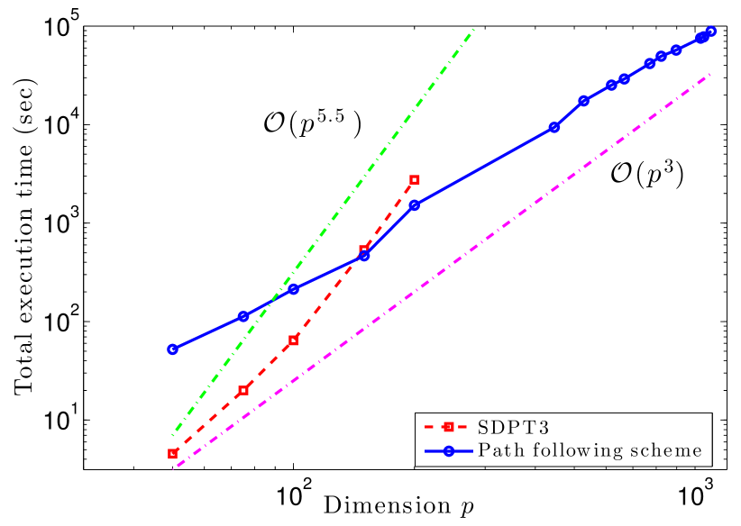
	SDPT3		​​PF scheme​​
$p$	​​variables​​	​​constraints​​	​​variables​​
$50$	$15.1$	$2.6$	$10$
$75$	$33.9$	$5.8$	$22.5$
$100$	$60.2$	$10.2$	$40$
$150$	$135.3$	$22.8$	$90$
$200$	$240.4$	$40.4$	$160$

Fig. 3: (Left) Execution times. (Right) Number of variables and equality constraints in thousands.

In terms of solution accuracy, our scheme with the aforementioned parameter settings is comparable to the low-precision mode of SDPT3, and can often obtain accurate solutions (cf., Table 2). However, Figure 3(Left) illustrates that our path following scheme has a rather dramatic scaling advantage as compared to SDPT3: $\mathcal{O}(p^{3})$ for ours vs. $\mathcal{O}(p^{5.5})$ for SDPT3. Because of this scaling, SDPT3 cannot handle problems instances where $p>200$ in our computer.

Reasons for our scalability are twofold. First, our path following scheme avoids “lifting” the problem into higher dimensions. Hence, as the problem dimensions grow (cf., Fig. 3(Right); numbers are in thousands), our memory requirement scales in a better fashion. Moreover, we do not have to handle additional (in)equality constraints. Second, the subproblem solver has linear convergence rate due to its construction (i.e., $\nabla^{2}f\succ 0$). Hence, our fast solver (FISTA) obtains medium accuracy solutions quickly since the proximal operator is efficient and has a closed form, and a warm-start strategy is used.

We also compare the proposed scheme with the scalable Factorization Method (FM), presented in [24]: a state-of-the-art, non-convex implementation of (3), based on splitting techniques. The code is publicly available at http://www.ali-jalali.com/. We modified this code to include a stopping criterion at a tolerance of

$$\left\|\mathbf{K}_{t_{k+1}}-\mathbf{K}_{t_{k}}\right\|_{F}\leq 10^{-8}\max\left\{\left\|\mathbf{K}_{t_{k}}\right\|_{F},1\right\}.$$

In Table 2, we report the average results of $10$ Monte-Carlo realizations for different $p$’s. While the non-convex approach exhibits lower computational complexity empirically, its solution quality suffers as compared to the convex solution, which has theoretical guarantees. It is clear that the non-convex approach is rather susceptible to local minima.

6.5 Sparse Pareto frontier in sparse graph learning

Many machine learning and signal processing problems naturally feature composite minimization problems where $f$ is directly self-concordant, such as sparse regression with unknown noise variance [43], Poisson imaging [22], one-bit compressive sensing, and graph learning [38, 26]. Here, we consider the graph learning problem: Let $\mathbf{\Sigma}$ be the covariance matrix of a Gaussian Markov random field (GMRF) and let $\mathbf{X}=\mathbf{\Sigma}^{-1}$. To satisfy the conditional dependencies with respect to the GMRF, $\mathbf{X}$ must have zero in $\mathbf{X}_{ij}$ corresponding to the absence of an edge between node $i$ and node $j$ [15]. Hence, given the empirical covariance $\widehat{\mathbf{\Sigma}}\succeq 0$, which is possibly rank deficient, we would like to learn the underlying GMRF.

It turns out that we can still learn GMRF’s with theoretical consistency guarantees from a number of data samples as few as $m=\mathcal{O}(d^{2}\log p)$ [38], where $d$ is the graph node degree, via

(52) $$\min_{\mathbf{X}\in\mathbb{R}^{p\times p}:~{}\mathbf{X}\succ 0}\left\{-\log\det(\mathbf{X})+\mathrm{tr}\left(\widehat{\mathbf{\Sigma}}\mathbf{X}\right)+\rho\left\|\mathrm{vec}\left(\mathbf{X}\right)\right\|_{1}\right\},$$

where $\rho>0$ is a regularization parameter. We easily observe that (52) satisfies the $\mathcal{P}(t)$ formulation for $t=1/\rho$. Unfortunately, the theoretical results only indicate the existence of a regularization parameter for consistent estimates and we have to tune to obtain the best $\rho^{*}$ in practice. We note that the function $f(\mathbf{X}):=-\log\det(\mathbf{X})$ is a self-concordant barrier of $\mathcal{S}^{p}_{+}$. As discussed in Subsection 6.1, we can modify the update rule for $\rho_{k}$, we can still apply Algorithm 1 to track the Pareto frontier of problem (52) for the case $f(\cdot)+\langle{\mathbf{c},\cdot}\rangle$ instead of $f(\cdot)$, see, e.g., [36].

To the best of our knowledge, the selection of $\rho^{\ast}$ with respect to a general-purpose objective, such as $\mathcal{P}(\rho)$, still remains widely open. For GMRF learning, a homotopy approach is proposed in [29, 42], where $\rho$ is updated by a non-adaptive multiplicative factor such that $\rho_{k+1}=c\rho_{k}$ for $0<c<1$. This approach is usually time consuming in practice, and may skip solutions with sparsity close to the desired sparsity level. Traditionally, (52) is addressed by IPM’s. Other than [47] exploited here, we do not know any scalable method that has rigorous global convergence guarantees for (52) as it has a globally non-Lipschitz continuous gradient. The authors in [3] use a probabilistic heuristic to select $\rho$: as the number of samples go to infinity, this heuristic leads to the maximum likelihood (unregularized) estimator. In practice though, the proposed $\rho$ values are quite large and do not consistently lead to good solutions.

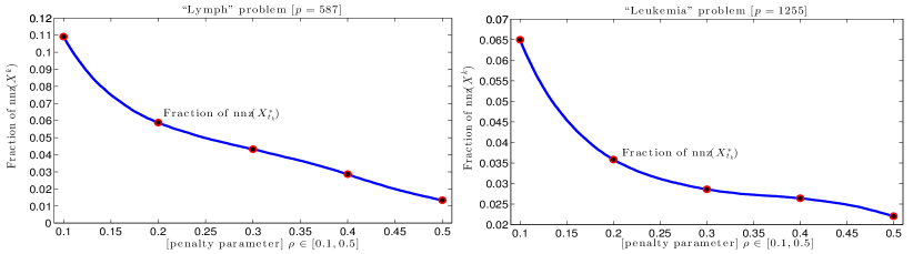
Fig. 4: Impact of the regularization parameter to the solution sparsity.

To this end, our scheme provides an adaptive strategy on how to update the regularization parameter. For instance, we can pick a range $\rho\in[\rho_{\text{min}},\rho_{0}]$ and apply our path-following scheme, starting from $\rho_{0}$ until we either achieve the desired solution sparsity or we reach the lower bound $\rho_{\text{min}}$. To illustrate the approach, we choose two real data examples from http://ima.umn.edu/~maxxa007/send_SICS/: Lymph and Leukemia, where the GMRF sizes are $p=587$ and $1255$, respectively. Figure 4 shows the solution sparsity vs. the penalty parameter curve (not to be confused with $f$ vs. $g$ curve, which is a convex Pareto curve) as obtained in a tuning-free fashion by our scheme.

In order to verify the obtained Pareto curve $\left\{\mathbf{X}^{k}_{\rho_{k}}\right\}$ well approximates the true solution trajectory $\mathbf{X}^{*}(\rho)$ of the problem (52), we apply the proximal-Newton algorithm in [46] to compute the approximate solution $\widetilde{\mathbf{X}}(\rho_{k})$ to $\mathbf{X}^{*}(\rho_{k})$ at five different points of $\rho$. The relative errors $e_{k}:=\left\|\mathbf{X}_{\rho_{k}}-\widetilde{\mathbf{X}}(\rho_{k})\right\|_{F}/\max\left\{\widetilde{\mathbf{X}}(\rho_{k})\right\}$ as well as the number of nonzero elements n.n.z. are shown in Table 3.

Table 3: The relative error and the number of nonzero elements of two approximate solutions

$\rho$	0.1	0.2	0.3	0.4	0.5
Lymph $(n=587)$
​​​Relative error $e_{k}$​​​	​​​0.0011​​​	​​​0.0013​​​	​​​0.0018​​​	​​​0.0018​​​	​​​$7.5342\times 10^{-6}$​​​
​​​n.n.z. ($\widetilde{\mathbf{X}}(\rho_{k})/\mathbf{X}_{\rho_{k}}$)​​​	​​​37587/37561​​​	​​​20275/20269​​​	​​​14901/14875​​​	​​​9869/9871​​​	​​​4615/4615​​​
Leukemia $(n=1255)$
​​​Relative error $e_{k}$​​​	​​​$6.1643\times 10^{-4}$​​​	​​​$5.5701\times 10^{-4}$​​​	​​​$6.2124\times 10^{-4}$​​​	​​​$5.6060\times 10^{-4}$​​​	​​​$3.6497\times 10^{-6}$​​​
​​​n.n.z. ($\widetilde{\mathbf{X}}(\rho_{k})/\mathbf{X}_{\rho_{k}}$)​​​	​​​102313/102253​​​	​​​56451/56421​​​	​​​45051/45055​​​	​​​41613/41609​​​	​​​34761/34761​​​

We can see from this table that both solutions are relatively close to each other both in terms of relative error and the sparsity.

7 Concluding remarks

We have proposed a new inexact path-following framework for minimizing (possibly) non-smooth and non-Lipschitz gradient objectives under constraints that admit a self-concordant barrier. We have shown how to solve such problems without lifting problem dimensions via additional slack variables and constraints. Our method is quite modular: custom implementations only require the corresponding custom solver for the composite subproblem (24) with a strongly convex quadratic smooth term and a tractable proximity of the second term $g$. We have provided a rigorous analysis that establish the worst-case analytical complexity of our approach via a new joint treatment of proximal methods and self-concordant optimization schemes. While our scheme maintains the original problem structure, its worst-case analytical complexity of the outer loop remains the same as in standard path-following interior point methods [31]. However, the overall complexity of the algorithm depends on the solution of the subproblem (24). We have also shown how the new scheme can obtain points on the Pareto frontier of regularized problems (with globally non-Lipschitz gradient of the smooth part $f$). We have numerically illustrated our method on three examples involving the nonsmooth constrained convex programming problems of matrix variables. Numerical results have shown that the new path-following scheme is superior to some off-the-self IP solvers such as SeDuMi and SDPT3 that require to transform the problem into standard conic programs.

8 Acknowledgment

The authors are also grateful to the anonymous reviewers as well as to the associate editor for their thorough comments and suggestions on improving the content and the presentation of this paper. This work was supported in part by the European Commission under Grant MIRG-268398, ERC Future Proof and SNF 200021-132548, SNF 200021-146750 and SNF CRSII2-147633.

Appendix A Technical proofs

We provide in this appendix the full proofs of two theorems: Theorem 8 and Theorem 10, and three technical lemmas: Lemma 11, Lemma 12 and Lemma 14.

A.1 The proof of Theorem 8

We define the restricted approximate gap between $\nabla^{2}f(\mathbf{x}^{*}_{t})$ and $\nabla^{2}f(\mathbf{x}_{t})$ along the direction $\bar{\mathbf{x}}^{+}_{t}-\mathbf{x}_{t}$ as $\bar{\mathbf{r}}_{t}:=(\nabla^{2}f(\mathbf{x}^{*}_{t})-\nabla^{2}f(\mathbf{x}_{t}))(\bar{\mathbf{x}}^{+}_{t}-\mathbf{x}_{t})$. Then, by using the definition (6) of $P_{\mathbf{x}}^{g}$ and (7) of $S_{\mathbf{x}}$, we can write (17) equivalently to

(53) $$\bar{\mathbf{x}}^{+}_{t}=P^{g}_{\mathbf{x}^{*}_{t}}\left(S_{\mathbf{x}^{*}_{t}}(\mathbf{x}_{t})+\bar{\mathbf{r}}_{t};t\right).$$

Now, we can estimate $\bar{\lambda}^{+}_{t}:=\left\|\bar{\mathbf{x}}^{+}_{t}-\mathbf{x}^{*}_{t}\right\|_{\mathbf{x}^{*}_{t}}$ as follows

$$\bar{\lambda}^{+}_{t} :=\left\|\bar{\mathbf{x}}^{+}_{t}-\mathbf{x}^{*}_{t}\right\|_{\mathbf{x}^{*}_{t}}$$

$$\overset{\tiny\eqref{eq:opt_cond_subprob1}+\eqref{eq:fixed_point_xstar}}{=}\left\|P^{g}_{\mathbf{x}^{*}_{t}}\left(S_{\mathbf{x}^{*}_{t}}(\mathbf{x}_{t})+\bar{\mathbf{r}}_{t};t\right)-P^{g}_{\mathbf{x}^{*}_{t}}\left(S_{\mathbf{x}^{*}_{t}}(\mathbf{x}^{*}_{t});t\right)\right\|_{\mathbf{x}^{*}_{t}}$$

$$\overset{\tiny\eqref{eq:nonexapansiveness}}{\leq}\left\|S_{\mathbf{x}^{*}_{t}}(\mathbf{x}_{t})-S_{\mathbf{x}^{*}_{t}}(\mathbf{x}^{*}_{t})+\bar{\mathbf{r}}_{t}\right\|_{\mathbf{x}^{*}_{t}}^{*}$$

(54) $$\leq\left\|S_{\mathbf{x}^{*}_{t}}(\mathbf{x}_{t})-S_{\mathbf{x}^{*}_{t}}(\mathbf{x}^{*}_{t})\right\|_{\mathbf{x}^{*}_{t}}^{*}+\left\|\bar{\mathbf{r}}_{t}\right\|_{\mathbf{x}^{*}_{t}}^{*}.$$

Similarly to the proof of [31, Theorem 4.1.14] or [46, Theorem 5], we show that

(55) $$\left\|S_{\mathbf{x}^{*}_{t}}(\mathbf{x}_{t})-S_{\mathbf{x}^{*}_{t}}(\mathbf{x}^{*}_{t})\right\|_{\mathbf{x}^{*}_{t}}^{*}\leq\frac{\lambda_{t}^{2}}{1-\lambda_{t}},$$

provided that $\lambda_{t}<1$.

Next, we estimate $\left\|\bar{\mathbf{r}}_{t}\right\|_{\mathbf{x}^{*}_{t}}^{*}$. We have

$$\left\|\bar{\mathbf{r}}_{t}\right\|_{\mathbf{x}^{*}_{t}}^{*} =\big{\|}\big{(}\nabla^{2}{f}(\mathbf{x}^{*}_{t})-\nabla^{2}f(\mathbf{x}_{t})\big{)}(\bar{\mathbf{x}}^{+}_{t}-\mathbf{x}_{t})\big{\|}_{\mathbf{x}^{*}_{t}}^{\ast}$$

$$\leq\left\|\nabla^{2}f(\mathbf{x}_{t}^{\ast})^{-1/2}\big{(}\nabla^{2}{f}(\mathbf{x}^{*}_{t})-\nabla^{2}f(\mathbf{x}_{t})\big{)}\nabla^{2}f(\mathbf{x}_{t}^{\ast})^{-1/2}\right\|_{2\rightarrow 2}\left\|\bar{\mathbf{x}}^{+}_{t}-\mathbf{x}_{t}\right\|_{\mathbf{x}^{\ast}_{t}}$$

(56) $$=\left\|\mathbb{I}-\nabla^{2}f(\mathbf{x}_{t}^{\ast})^{-1/2}\nabla^{2}f(\mathbf{x}_{t})\nabla^{2}f(\mathbf{x}_{t}^{\ast})^{-1/2}\right\|_{2\rightarrow 2}\left\|\bar{\mathbf{x}}^{+}_{t}-\mathbf{x}_{t}\right\|_{\mathbf{x}^{\ast}_{t}},$$

where $\left\|\cdot\right\|_{2\to 2}$ is the $\ell_{2}$-norm of a matrix, i.e., $\left\|\mathbf{X}\right\|_{2\to 2}:=\max_{\mathbf{u}}\left\{\left\|\mathbf{X}\mathbf{u}\right\|_{2}~{}|~{}\left\|\mathbf{u}\right\|_{2}=1\right\}$ for a given matrix $\mathbf{X}$. By applying [31, Theorem 4.1.6], we can show that

$$\Big{\|}\mathbb{I}-\nabla^{2}f(\mathbf{x}_{t}^{\ast})^{-1/2}\nabla^{2}f(\mathbf{x}_{t})\nabla^{2}f(\mathbf{x}_{t}^{\ast})^{-1/2}\Big{\|}_{2\rightarrow 2} \leq\max\left\{1-(1-\lambda_{t})^{2},(1-\lambda_{t})^{-2}-1\right\}$$

$$=\frac{2\lambda_{t}-\lambda_{t}^{2}}{(1-\lambda_{t})^{2}}.$$

Substituting this estimate into (A.1) and then using the triangle inequality, we obtain

(57) $$\left\|\bar{\mathbf{r}}_{t}\right\|_{\mathbf{x}^{*}_{t}}\leq\left(\frac{2\lambda_{t}-\lambda_{t}^{2}}{(1-\lambda_{t})^{2}}\right)\left\|\bar{\mathbf{x}}^{+}_{t}-\mathbf{x}_{t}\right\|_{\mathbf{x}^{*}_{t}}\leq\left(\frac{2\lambda_{t}-\lambda_{t}^{2}}{(1-\lambda_{t})^{2}}\right)\left(\bar{\lambda}_{t}^{+}+\lambda_{t}\right),$$

provided that $\lambda_{t}<1$.

Substituting (55) and (57) into (A.1) and then rearranging the result, we deduce

(58) $$\bar{\lambda}_{t}^{+}\leq\left(\frac{3-2\lambda_{t}}{1-4\lambda_{t}+2\lambda_{t}^{2}}\right)\lambda_{t}^{2},$$

provided that $1-4\lambda_{t}+2\lambda_{t}^{2}>0$. We can easily show that the condition $1-4\lambda_{t}+2\lambda_{t}^{2}>0$ holds if $\lambda_{t}\in[0,1-\frac{\sqrt{2}}{2})$.

Note that $0\preceq\nabla^{2}f(\mathbf{x}^{*}_{t})\preceq(1-\lambda_{t})^{-2}\nabla^{2}f(\mathbf{x}_{t})$ due to [31, Theorem 4.1.6]. Thus, for any $\mathbf{u}$, we have $\left\|\mathbf{u}\right\|_{\mathbf{x}^{*}_{t}}\leq(1-\lambda_{t})^{-1}\left\|\mathbf{u}\right\|_{\mathbf{x}_{t}}$. By using this inequality, (20) and the triangle inequality, it is easy to show that

$$\lambda_{t}^{+} =\left\|\mathbf{x}^{+}_{t}-\mathbf{x}^{*}_{t}\right\|_{\mathbf{x}^{*}_{t}}\leq\left\|\mathbf{x}^{+}_{t}-\bar{\mathbf{x}}^{+}_{t}\right\|_{\mathbf{x}^{*}_{t}}+\left\|\bar{\mathbf{x}}^{+}_{t}-\mathbf{x}^{*}_{t}\right\|_{\mathbf{x}^{*}_{t}}$$

$$\overset{\tiny\eqref{eq:computable_criterion2}}{\leq}(1-\lambda_{t})^{-1}\delta_{k}+\bar{\lambda}_{t}^{+}.$$

By substituting (58) into this inequality, we obtain

(59) $$\lambda_{t}^{+}\leq\frac{\delta_{k}}{1-\lambda_{t}}+\left(\frac{3-2\lambda_{t}}{1-4\lambda_{t}+2\lambda_{t}^{2}}\right)\lambda_{t}^{2}.$$

Since $\lambda_{t}\in[0,1-\frac{\sqrt{2}}{2})$, the right-hand side of (59) is well-defined. Moreover, it is obvious to check that the right-hand side of (59) is increasing w.r.t. $\delta_{k}\geq 0$ and $\lambda_{t}\in[0,1-\frac{\sqrt{2}}{2})$. $\square$

A.2 The proof of Theorem 10

We define the function $\psi(\lambda):=\frac{3-2\lambda}{1-4\lambda+2\lambda^{2}}$. It is easy to check that $\psi$ is increasing in $[0,1-\sqrt{2}/2)$. Let us limit the range of $\lambda\in[0,0.15]$. Then, one can show that $\max\left\{\psi(\lambda)~{}|~{}\lambda\in[0,0.15]\right\}\leq 6.07$. Hence, we can upper estimate (25) by some elementary calculations to obtain

(60) $$\lambda_{t_{k+1}}^{+}\leq 1.18\delta_{k}+6.07\lambda_{t_{k+1}}^{2}.$$

Now, we recall the following estimate from [48, Lemma A.1.(c)] as

(61) $${}\lambda_{t_{k+1}}\leq\frac{\lambda_{t_{k}}^{+}+\Delta_{k}}{1-\Delta_{k}},$$

provided that $\Delta_{k}<1$.

Let us fix some $\beta\in(0,0.15]$. By the assumption $\lambda_{t_{k}}^{+}\leq\beta$, it follows from (61) that

(62) $$\lambda_{t_{k+1}}\leq\frac{\lambda_{t_{k}}^{+}+\Delta_{k}}{1-\Delta_{k}}\leq\frac{\beta+\Delta_{k}}{1-\Delta_{k}}.$$

Substituting (62) into (60) we obtain

(63) $$\lambda_{t_{k+1}}^{+}\leq 1.18\delta_{k}+6.07\left(\frac{\beta+\Delta_{k}}{1-\Delta_{k}}\right)^{2}.$$

Since we desire $\lambda_{t_{k+1}}^{+}\leq\beta$, by using (63), we require $\left(\frac{\beta+\Delta_{k}}{1-\Delta_{k}}\right)^{2}\leq\frac{\beta-1.18\delta_{k}}{6.07}$ provided that $\delta_{k}<\beta/1.18$. Since $\delta_{k}\leq 0.075\beta$, the last condition leads to

(64) $$0\leq\Delta_{k}\leq\frac{\sqrt{\beta}-2.581\beta}{2.581+\sqrt{\beta}}<1,$$

for any $\beta\in(0,0.15]$. Finally, we can easy check that $\lambda_{t_{k+1}}\leq\frac{1}{2.581}\sqrt{\beta}$ for $k\geq 0$ due to (60). $\square$

A.3 The proof of Lemma 11

Since $\mathbf{x}^{*}_{t_{k}}$ and $\mathbf{x}^{*}_{t_{k+1}}$ are the solutions of (2) at $t=t_{k}$ and $t=t_{k+1}$, respectively, they satisfy the following optimality conditions:

$$\mathbf{0}\in t_{k}\nabla{f}(\mathbf{x}^{*}_{t_{k}})+\partial{g}(\mathbf{x}^{*}_{t_{k}}),$$

$$\mathbf{0}\in t_{k+1}\nabla{f}(\mathbf{x}^{*}_{t_{k+1}})+\partial{g}(\mathbf{x}^{*}_{t_{k+1}}).$$

Hence, there exist $\mathbf{v}_{k}\in\partial{g}(\mathbf{x}^{*}_{t_{k}})$ and $\mathbf{v}_{k+1}\in\partial{g}(\mathbf{x}^{*}_{t_{k+1}})$ such that $\mathbf{v}_{k}=-t_{k}\nabla{f}(\mathbf{x}^{*}_{t_{k}})$ and $\mathbf{v}_{k+1}=-t_{k+1}\nabla{f}(\mathbf{x}^{*}_{t_{k+1}})$. Then, we have

$$\mathbf{v}_{k+1}-\mathbf{v}_{k} =t_{k}\nabla{f}(\mathbf{x}^{*}_{t_{k}})-t_{k+1}\nabla{f}(\mathbf{x}^{*}_{t_{k+1}})$$

$$\overset{\tiny\eqref{eq:update_t}}{=}t_{k}\left(\nabla{f}(\mathbf{x}^{*}_{t_{k}})-\nabla{f}(\mathbf{x}^{*}_{t_{k+1}})\right)-d_{k}\nabla{f}(\mathbf{x}^{*}_{t_{k+1}}).$$

By using the convexity of $g$, the last expression implies

$$0 \leq(\mathbf{v}_{k+1}-\mathbf{v}_{k})^{T}(\mathbf{x}^{*}_{t_{k+1}}-\mathbf{x}^{*}_{t_{k}})$$

$$=t_{k}\left(\nabla{f}(\mathbf{x}^{*}_{t_{k}})-\nabla{f}(\mathbf{x}^{*}_{t_{k+1}})\right)^{T}(\mathbf{x}^{*}_{t_{k+1}}-\mathbf{x}^{*}_{t_{k}})-d_{k}\nabla{f}(\mathbf{x}^{*}_{t_{k+1}})^{T}(\mathbf{x}^{*}_{t_{k+1}}-\mathbf{x}^{*}_{t_{k}})$$

$$\leq t_{k}\left(\nabla{f}(\mathbf{x}^{*}_{t_{k}})-\nabla{f}(\mathbf{x}^{*}_{t_{k+1}})\right)^{T}(\mathbf{x}^{*}_{t_{k+1}}-\mathbf{x}^{*}_{t_{k}})+\left|d_{k}\right|\|\nabla{f}(\mathbf{x}^{*}_{t_{k+1}})\|_{\mathbf{x}^{*}_{t_{k+1}}}^{*}\|\mathbf{x}^{*}_{t_{k+1}}-\mathbf{x}^{*}_{t_{k}}\|_{\mathbf{x}^{*}_{t_{k+1}}},$$

where the last inequality is due to the generalized Cauchy-Schwatz inequality. Since $t_{k}>0$, we further have

(65) $$\left(\nabla{f}(\mathbf{x}^{*}_{t_{k+1}})-\nabla{f}(\mathbf{x}^{*}_{t_{k}})\right)^{T}(\mathbf{x}^{*}_{t_{k+1}}-\mathbf{x}^{*}_{t_{k}})\leq\frac{\left|d_{k}\right|}{t_{k}}\|\nabla{f}(\mathbf{x}^{*}_{t_{k+1}})\|_{\mathbf{x}^{*}_{t_{k+1}}}^{*}\|\mathbf{x}^{*}_{t_{k+1}}-\mathbf{x}^{*}_{t_{k}}\|_{\mathbf{x}^{*}_{t_{k+1}}}.$$

However, since $f$ is standard self-concordant, by applying [31, Theorem 4.1.7], we have

$$\left(\nabla{f}(\mathbf{x}^{*}_{t_{k+1}})-\nabla{f}(\mathbf{x}^{*}_{t_{k}})\right)^{T}(\mathbf{x}^{*}_{t_{k+1}}-\mathbf{x}^{*}_{t_{k}})\geq\frac{\|\mathbf{x}^{*}_{t_{k+1}}-\mathbf{x}^{*}_{t_{k}}\|_{\mathbf{x}^{*}_{t_{k+1}}}^{2}}{1+\|\mathbf{x}^{*}_{t_{k+1}}-\mathbf{x}^{*}_{t_{k}}\|_{\mathbf{x}^{*}_{t_{k+1}}}}.$$

Using this inequality together with (65) we obtain

$$\frac{\|\mathbf{x}^{*}_{t_{k+1}}-\mathbf{x}^{*}_{t_{k}}\|_{\mathbf{x}^{*}_{t_{k+1}}}}{1+\|\mathbf{x}^{*}_{t_{k+1}}-\mathbf{x}^{*}_{t_{k}}\|_{\mathbf{x}^{*}_{t_{k+1}}}} \leq\frac{\left|d_{k}\right|}{t_{k}}\|\nabla{f}(\mathbf{x}^{*}_{t_{k+1}})\|_{\mathbf{x}^{*}_{t_{k+1}}}^{*}\overset{\tiny\eqref{eq:used}}{\leq}\frac{\left|d_{k}\right|}{t_{k}}\sqrt{\nu}.$$

where by the definition of $\Delta_{k}$, this completes the proof of (28). The last statement in Lemma 11 is a direct consequence of (28). $\square$

A.4 The proof of Lemma 12

Let $g_{0}(\cdot):=t^{-1}_{0}g(\cdot)$. Similar to the proof of [46, Lemma 3.3], we can estimate

(66) $$F(\mathbf{x}^{j+1}_{t_{0}};t_{0})-F(\mathbf{x}^{j}_{t_{0}};t_{0})\leq-\alpha_{j}\nabla{f}(\mathbf{x}^{j}_{t_{0}})^{T}\mathbf{d}^{j}+\omega_{*}(\alpha_{j}\zeta_{j})+\alpha_{j}\left(g_{0}(\mathbf{s}^{j}_{t_{0}})-g_{0}(\mathbf{x}^{j}_{t_{0}})\right),$$

where $\alpha_{j}\zeta_{j}<1$ and $\omega_{*}(\tau):=-\tau-\ln(1-\tau)$. From the definition (13) of $\widehat{F}$ and (32) we have

$$g_{0}(\mathbf{s}^{j}_{t_{0}})-g_{0}(\mathbf{x}^{j}_{t_{0}}) \leq g_{0}(\bar{\mathbf{s}}^{j}_{t_{0}})-g_{0}(\mathbf{x}^{j}_{t_{0}})+\frac{(\delta_{0}^{j})^{2}}{2}+\nabla{f}(\mathbf{x}^{j}_{t_{0}})^{T}(\bar{\mathbf{s}}^{j}_{t_{0}}-\mathbf{s}^{j}_{t_{0}})$$

(67) $$+\frac{1}{2}\left(\left\|\bar{\mathbf{s}}^{j}-\mathbf{x}^{j}\right\|_{\mathbf{x}^{j}}^{2}-\left\|\mathbf{s}^{j}-\mathbf{x}^{j}\right\|_{\mathbf{x}^{j}}^{2}\right).$$

Since $\bar{\mathbf{s}}^{j}_{t_{0}}$ is the exact solution of (31), using the optimality condition (17) of this problem, we have

(68) $$\bar{\mathbf{v}}^{j}_{t_{0}}=-\nabla{f}(\mathbf{x}^{j}_{t_{0}})-\nabla^{2}f(\mathbf{x}^{j}_{t_{0}})(\bar{\mathbf{s}}^{j}_{t_{0}}-\mathbf{x}^{j}_{t_{0}}),~{}\bar{\mathbf{v}}^{j}_{t_{0}}\in\partial{g}_{0}(\bar{\mathbf{s}}^{j}_{t_{0}}).$$

By the convexity of $g_{0}$, (68) implies

$$g_{0}(\bar{\mathbf{s}}^{j}_{t_{0}})-g_{0}(\mathbf{x}^{j}_{t_{0}})\leq-\nabla{f}(\mathbf{x}^{j}_{t_{0}})^{T}(\bar{\mathbf{s}}^{j}_{t_{0}}-\mathbf{x}^{j}_{t_{0}})-\|\bar{\mathbf{s}}^{j}_{t_{0}}-\mathbf{x}^{j}_{t_{0}}\|_{\mathbf{x}^{j}_{t_{0}}}^{2}.$$

Substituting this inequality into (A.4) and rearranging the result by using $\zeta_{j}=\|\mathbf{d}^{j}_{t_{0}}\|_{\mathbf{x}^{j}_{t_{0}}}=\|\mathbf{s}^{j}_{t_{0}}-\mathbf{x}^{j}_{t_{0}}\|_{\mathbf{x}^{j}_{t_{0}}}$, we obtain

(69) $$g_{0}(\mathbf{s}^{j}_{t_{0}})-g_{0}(\mathbf{x}^{j}_{t_{0}})\leq\frac{(\delta^{j}_{0})^{2}}{2}-\nabla{f}(\mathbf{x}^{j}_{t_{0}})^{T}(\mathbf{s}^{j}_{t_{0}}-\mathbf{x}^{j}_{t_{0}})-\frac{1}{2}\left(\|\bar{\mathbf{s}}^{j}_{t_{0}}-\mathbf{x}^{j}_{t_{0}}\|_{\mathbf{x}^{j}_{t_{0}}}^{2}+\zeta_{j}^{2}\right).$$

By using the triangle inequality and (19) we deduce

$$\|\bar{\mathbf{s}}^{j}_{t_{0}}-\mathbf{x}^{j}_{t_{0}}\|_{\mathbf{x}^{j}_{t_{0}}}\geq\|\mathbf{s}^{j}_{t_{0}}-\mathbf{x}^{j}_{t_{0}}\|_{\mathbf{x}^{j}_{t_{0}}}-\|\mathbf{s}^{j}_{t_{0}}-\bar{\mathbf{s}}^{j}_{t_{0}}\|_{\mathbf{x}^{j}_{t_{0}}}\geq\zeta_{j}-\delta^{j}_{0}.$$

Hence, with $\delta^{j}_{0}\leq\zeta_{j}$, this inequality implies

(70) $$\|\bar{\mathbf{s}}^{j}_{t_{0}}-\mathbf{x}^{j}_{t_{0}}\|_{\mathbf{x}^{j}_{t_{0}}}^{2}\geq\zeta_{j}^{2}+(\delta^{j}_{0})^{2}-2\zeta_{j}\delta^{j}_{0}.$$

Combining (66), (69) and (70), we finally get

(71) $$F(\mathbf{x}^{j+1}_{t_{0}};t_{0})-F(\mathbf{x}^{j}_{t_{0}};t_{0})\leq\omega_{*}(\alpha_{j}\zeta_{j})-\zeta_{j}(\zeta_{j}-\delta_{0}^{j})\alpha_{j},$$

provided that $\alpha_{j}\zeta_{j}<1$ and $\delta^{j}_{0}\leq\zeta_{j}$.

Now we consider the function $\varphi(\alpha):=\zeta_{j}(\zeta_{j}-\delta_{0}^{j})\alpha-\omega_{*}(\zeta_{j}\alpha)$. This function is concave, it attains the maximum at $\alpha_{j}:=\frac{\zeta_{j}-\delta^{j}_{0}}{\zeta_{j}(1+\zeta_{j}-\delta^{j}_{0})}$ provided that $\delta^{j}_{0}\leq\zeta_{j}$. In this case, we also have $\alpha_{j}\zeta_{j}=\frac{\zeta_{j}-\delta^{j}_{0}}{1+\zeta_{j}-\delta^{j}_{0}}<1$ and $\varphi(\alpha_{j})=\omega(\zeta_{j}-\delta^{j}_{0})$. Substituting this value into (71), we obtain (33). $\square$

A.5 The proof of Lemma 14

Since $f$ is the barrier function of $\Omega$ and $\mathbf{x}^{*}_{t}$ is the solution of (2), it is obvious that $\mathbf{x}^{*}_{t}\in\mathrm{int}(\Omega)$ and $g(\mathbf{x}^{*})\leq g(\mathbf{x}^{*}_{t})$. We first prove (38). From [31, Theorem 4.2.4] we have

(72) $$\nabla{f}(\mathbf{x})^{T}(\mathbf{y}-\mathbf{x})<\nu,~{}~{}\forall\mathbf{x},\mathbf{y}\in\mathrm{dom}\left(f\right).$$

By using the convexity of $g$, the optimality condition (5) and the property (72) of the barrier function $f$, for any $\mathbf{x}\in\mathrm{dom}\left(F\right)\equiv\mathrm{dom}\left(f\right)\cap\mathrm{dom}\left(g\right)$, we have

$$g(\mathbf{x})-g(\mathbf{x}^{*}_{t}) \geq(\xi^{*}_{t})^{T}(\mathbf{x}-\mathbf{x}^{*}_{t}),~{}~{}\xi^{*}_{t}\in\partial{g}(\mathbf{x}^{*}_{t})$$

(73) $$\overset{\tiny\eqref{eq:optimality_for_ln_barrier}}{\geq}-t\nabla{f}(\mathbf{x}^{*}_{t})^{T}(\mathbf{x}-\mathbf{x}^{*}_{t})$$

$$\overset{\tiny\eqref{eq:property_barrier1}}{\geq}-t\nu.$$

By substituting $\mathbf{x}=\mathbf{x}^{*}$ in (A.5) we obtain (38). Since $\mathbf{x}_{t_{k}}\in\Omega$ and $\mathbf{x}^{*}_{t}$ is the optimal solution of Similarly, by letting $t=t_{k}$ and $\mathbf{x}=\mathbf{x}_{t_{k}}$ in (A.5) we obtain the left-hand side of (39).

Next, we prove the right-hand side of (39). By using (18) in Definition 6 we can estimate

$$g(\mathbf{x}_{t_{k}}) \leq g(\bar{\mathbf{x}}_{t_{k}})+t_{k}\left[Q(\bar{\mathbf{x}}_{t_{k}};\mathbf{x}_{t_{k-1}})-Q(\mathbf{x}_{t_{k}};\mathbf{x}_{t_{k-1}})\right]+t_{k}\frac{\delta_{k}^{2}}{2}$$

$$\leq g(\bar{\mathbf{x}}_{t_{k}})+t_{k}\nabla{f}(\mathbf{x}_{t_{k-1}})^{T}(\bar{\mathbf{x}}_{t_{k}}-\mathbf{x}_{t_{k}})+t_{k}\frac{\delta_{k}^{2}}{2}$$

(74) $$+\frac{t_{k}}{2}\left[\left\|\bar{\mathbf{x}}_{t_{k}}-\mathbf{x}_{t_{k-1}}\right\|^{2}_{\mathbf{x}_{t_{k-1}}}-\left\|\mathbf{x}_{t_{k}}-\mathbf{x}_{t_{k-1}}\right\|^{2}_{\mathbf{x}_{t_{k-1}}}\right],$$

where $\bar{\mathbf{x}}_{t_{k}}$ is the exact solution of (16) at $t=t_{k}$. Moreover, from the optimality condition (17), there exists $\bar{\mathbf{v}}_{k}\in\partial{g}(\bar{\mathbf{x}}_{t_{k}})$ such that

(75) $$\bar{\mathbf{v}}_{k}=-t_{k}\nabla{f}(\mathbf{x}_{t_{k-1}})-t_{k}\nabla^{2}{f}(\mathbf{x}_{t_{k-1}})(\bar{\mathbf{x}}_{t_{k}}-\mathbf{x}_{t_{k-1}}).$$

By using the convexity of $g$ we can estimate $g(\mathbf{x}^{*}_{t_{k}})-g(\mathbf{x}_{t_{k}})$ as

$$g(\mathbf{x}^{*}_{t_{k}})-g(\bar{\mathbf{x}}_{t_{k}}) \geq\bar{\mathbf{v}}_{k}^{T}(\mathbf{x}^{*}_{t_{k}}-\bar{\mathbf{x}}_{t_{k}})$$

$$\overset{\tiny\eqref{eq:lm31_proof1}}{=}-t_{k}\nabla{f}(\mathbf{x}_{t_{k-1}})^{T}(\mathbf{x}^{*}_{t_{k}}-\bar{\mathbf{x}}_{t_{k}})$$

(76) $$-t_{k}(\bar{\mathbf{x}}_{t_{k}}-\mathbf{x}_{t_{k-1}})^{T}\nabla^{2}{f}(\mathbf{x}_{t_{k-1}})(\mathbf{x}^{*}_{t_{k}}-\bar{\mathbf{x}}_{t_{k}}).$$

Now we sum up (A.5) and (A.5) and then rearrange the result by using the Cauchy-Schwarz inequality to get

$$g(\mathbf{x}^{*}_{t_{k}})-g(\mathbf{x}_{t_{k}}) \geq-t_{k}\nabla{f}(\mathbf{x}_{t_{k-1}})^{T}(\mathbf{x}^{*}_{t_{k}}-\mathbf{x}_{t_{k}})-\frac{t_{k}}{2}\delta_{k}^{2}$$

$$-\frac{t_{k}}{2}\Big{[}\|\bar{\mathbf{x}}_{t_{k}}-\mathbf{x}_{t_{k-1}}\|_{\mathbf{x}_{t_{k-1}}}^{2}-\|\mathbf{x}_{t_{k}}-\mathbf{x}_{t_{k-1}}\|_{\mathbf{x}_{t_{k-1}}}^{2}$$

(77) $$+2(\bar{\mathbf{x}}_{t_{k}}-\mathbf{x}_{t_{k-1}})^{T}\nabla^{2}f(\mathbf{x}_{t_{k-1}})(\mathbf{x}^{*}_{t_{k}}-\bar{\mathbf{x}}_{t_{k}})\Big{]}_{[1]}.$$

From [31, Theorem 4.1.6] we have

(78) $$(1-\lambda_{t_{k}})^{2}\nabla^{2}f(\mathbf{x}^{*}_{t_{k}})\preceq\nabla^{2}{f}(\mathbf{x}_{t_{k-1}})\preceq(1-\lambda_{t_{k}})^{-2}\nabla^{2}{f}(\mathbf{x}^{*}_{t_{k}}),$$

where $\lambda_{t_{k}}:=\|\mathbf{x}_{t_{k-1}}-\mathbf{x}^{*}_{t_{k}}\|_{\mathbf{x}^{*}_{t_{k}}}$ defined as before. We can easily show that

$$\left\|\nabla{f}(\mathbf{x}_{t_{k-1}})\right\|_{\mathbf{x}^{*}_{t_{k}}}^{*}\leq(1-\lambda_{t_{k}})^{-1}\left\|\nabla{f}(\mathbf{x}_{t_{k-1}})\right\|_{\mathbf{x}_{t_{k-1}}}^{*}\overset{\tiny\eqref{eq:used}}{\leq}(1-\lambda_{t_{k}})^{-1}\sqrt{\nu}.$$

Using this inequality together with the Cauchy-Shwarz inequality, we can prove that

$$\nabla{f}(\mathbf{x}_{t_{k-1}})^{T}(\mathbf{x}^{*}_{t_{k}}-\mathbf{x}_{t_{k}}) \leq\left\|\nabla{f}(\mathbf{x}_{t_{k-1}})\right\|_{\mathbf{x}^{*}_{t_{k}}}^{*}\left\|\mathbf{x}_{t_{k}}-\mathbf{x}^{*}_{t_{k}}\right\|_{\mathbf{x}^{*}_{t_{k}}}$$

(79) $$=\sqrt{\nu}(1-\lambda_{t_{k}})^{-1}\lambda_{t_{k}}^{+}.$$

Next, we estimate the last term $[\cdots]_{[1]}$ of (A.5) as follows

$$[\cdots]_{[1]} :=\|\bar{\mathbf{x}}_{t_{k}}-\mathbf{x}_{t_{k-1}}\|_{\mathbf{x}_{t_{k-1}}}^{2}-\|\mathbf{x}_{t_{k}}-\mathbf{x}_{t_{k-1}}\|_{\mathbf{x}_{t_{k-1}}}^{2}$$

$$+2(\bar{\mathbf{x}}_{t_{k}}-\mathbf{x}_{t_{k-1}})^{T}\nabla^{2}f(\mathbf{x}_{t_{k-1}})(\mathbf{x}^{*}_{t_{k}}-\bar{\mathbf{x}}_{t_{k}})$$

$$=-\left\|\mathbf{x}_{t_{k}}-\mathbf{x}_{t_{k-1}}\right\|_{\mathbf{x}_{t_{k-1}}}^{2}-\left\|\bar{\mathbf{x}}_{t_{k}}-\mathbf{x}_{t_{k-1}}\right\|_{\mathbf{x}_{t_{k-1}}}^{2}$$

$$+2(\bar{\mathbf{x}}_{t_{k}}-\mathbf{x}_{t_{k-1}})^{T}\nabla^{2}f(\mathbf{x}_{t_{k-1}})(\mathbf{x}^{*}_{t_{k}}-\mathbf{x}_{t_{k-1}})$$

$$\leq-\frac{1}{2}\left\|\bar{\mathbf{x}}_{t_{k}}-\mathbf{x}_{t_{k}}\right\|_{\mathbf{x}_{t_{k-1}}}^{2}+2(\bar{\mathbf{x}}_{t_{k}}-\mathbf{x}_{t_{k-1}})^{T}\nabla^{2}f(\mathbf{x}_{t_{k-1}})(\mathbf{x}^{*}_{t_{k}}-\mathbf{x}_{t_{k-1}})$$

$$\overset{\tiny\eqref{eq:lm51_est4c}}{\leq}2(1-\lambda_{t_{k}})^{-2}\left(\left\|\bar{\mathbf{x}}_{t_{k}}-\mathbf{x}_{t_{k}}\right\|_{\mathbf{x}_{t_{k-1}}}+\lambda_{t_{k}}^{+}+\lambda_{t_{k}}\right)\lambda_{t_{k}}$$

(80) $$\leq 2(1-\lambda_{t_{k}})^{-2}\left(\delta_{k}+\lambda_{t_{k}}^{+}+\lambda_{t_{k}}\right)\lambda_{t_{k}}.$$

Here, the two last inequalities are obtained by using the triangle inequality, the definition of $\lambda_{t_{k}}^{+}$, $\lambda_{t_{k}}$ and (20). Now, we combine (A.5), (A.5) and (A.5) to derive

$$g(\mathbf{x}^{*}_{t_{k}})-g(\mathbf{x}_{t_{k}}) \geq-t_{k}\left[\sqrt{\nu}\frac{\lambda_{t_{k}}^{+}}{1-\lambda_{t_{k}}}+(1-\lambda_{t_{k}})^{-2}\lambda_{t_{k}}\left(\lambda_{t_{k}}^{+}+\lambda_{t_{k}}+\delta_{k}\right)+\frac{\delta_{k}^{2}}{2}\right],$$

which is the right-hand side of (39) provided that $\lambda_{t_{k}}<1$. Finally, the estimate (40) follows directly by summing up (38) and (39). Here, the left-hand side of (40) follows from the fact that $\mathbf{x}_{t_{k}}\in\Omega$, and therefore, $g(\mathbf{x}_{t_{k}})-g(\mathbf{x}^{*})\geq 0$. $\square$

References

• [1] Andreasson, N., Evgrafov, A., and Patriksson, M. Introduction to Continuous Optimization: Foundations and Fundamental Algorithms. Studentlitteratur AB, 2006.
• [2] Banaszek, K., D’Ariano, G. M., Paris, M. G. A., and Sacchi, M. F. Maximum-likelihood estimation of the density matrix. Phys. Rev. A. 61, 010304 (1999), 1–4.
• [3] Banerjee, O., El Ghaoui, L., and d’Aspremont, A. Model selection through sparse maximum likelihood estimation for multivariate gaussian or binary data. The Journal of Machine Learning Research 9 (2008), 485–516.
• [4] Bansal, N., Blum, A., and Chawla, S. Correlation Clustering. Machine Learning 56 (2004), 89–113.
• [5] Bauschke, H., and Combettes, P. Convex analysis and monotone operators theory in Hilbert spaces. Springer-Verlag, 2011.
• [6] Beck, A., and Teboulle, M. Mirror descent and nonlinear projected subgradient methods for convex optimization. Operations Research Letters 31, 3 (2003), 167–175.
• [7] Beck, A., and Teboulle, M. A Fast Iterative Shrinkage-Thresholding Algorithm for Linear Inverse Problems. SIAM J. Imaging Sciences 2, 1 (2009), 183–202.
• [8] Becker, S., Bobin, J., and Candès, E. NESTA: a fast and accurate first-order method for sparse recovery. SIAM J. Imaging Science 4, 1 (2011), 1–39.
• [9] Ben-Tal, A., Margalit, T., and Nemirovski, A. The ordered subsets mirror descent optimization method with applications to tomography. SIAM J. Optim. 12 (2001), 79–108.
• [10] Ben-Tal, A., and Nemirovski, A. Lectures on Modern Convex Optimization: Analysis, Algorithms, and Engineering Applications, vol. 3 of MPS/SIAM Series on Optimization. SIAM, 2001.
• [11] Bhaskar, B., Tang, G., and Recht, B. Atomic norm denoising with applications to line spectral estimation. arXiv preprint arXiv:1204.0562 (2012), 1–27.
• [12] Bonnans, J., Gilbert, J., Lemarechal, C., and Sagastizabal, C. Numerical Optimization: Theoretical and Practical Aspects. Springer-Verlag, 1997.
• [13] Boyd, S., Ghaoui, L., Feron, E., and Balakrishnan, V. Linear matrix inequalities in system and control theory, vol. 14. SIAM, 1994.
• [14] Candes, E. J., Eldar, Y., Strohmer, T., and Voroninski, V. Phase retrieval via matrix completion. SIAM J. on Imaging Sciences 6, 1 (2011), 199–225.
• [15] Dempster, A. P. Covariance selection. Biometrics 28 (1972), 157–175.
• [16] Facchinei, F., and Pang, J.-S. Finite-dimensional variational inequalities and complementarity problems, vol. 1-2. Springer-Verlag, 2003.
• [17] Fiacco, A. Introduction to sensitivity and stability analysis in nonlinear programming. Academic Press, New York, 1983.
• [18] Fletcher, R. Practical Methods of Optimization, 2nd ed. Wiley, Chichester, 1987.
• [19] Grant, M., Boyd, S., and Ye, Y. Disciplined convex programming. In Global Optimization: From Theory to Implementation, L. Liberti and N. Maculan, Eds., Nonconvex Optimization and its Applications. Springer, 2006, pp. 155–210.
• [20] Guddat, J., Vasquez, F. G., and Jongen, H. Parametric Optimization: Singularities, Pathfollowing and Jumps. Teubner, Stuttgart, 1990.
• [21] Hale, E., Yin, W., and Zhang, Y. Fixed-point continuation for $\ell_{1}$-minimization: methodology and convergence. SIAM J. Optim. 19, 3 (2008), 1107–1130.
• [22] Harmany, Z., Marcia, R., and Willett, R. M. This is SPIRAL-TAP: Sparse Poisson Intensity Reconstruction Algorithms - Theory and Practice,. IEEE Transactions on Image Processing 21, 3 (2012), 1084–1096.
• [23] Hassibi, A., How, J., and Boyd, S. A path following method for solving bmi problems in control. In Proceedings of American Control Conference (1999), vol. 2, pp. 1385–1389.
• [24] Jalali, A., and Srebro, N. Clustering using max-norm constrained optimization. In Proc. of International Conference on Machine Learning (ICML2012) (2012), pp. 1–17.
• [25] Karas, E., Ribeiro, A., Sagastizabal, C., and Solodov, M. A bundle-filter method for nonsmooth convex constrained optimization. Math. Program. 116 (2009), 297–320.
• [26] Kyrillidis, A., and Cevher, V. Fast proximal algorithms for self-concordant function minimization with application to sparse graph selection. Proc. of the 38th International Conference on Acoustics, Speech, and Signal Processing (ICASSP) (2013), 1–5.
• [27] Lan, G. Bundle-level type methods uniformly optimal for smooth and nonsmooth convex optimization. Math. Program. DOI 10.1007/s10107-013-0737-x (2013), 1–45.
• [28] Lemarechal, C., Nemirovskii, A., and Nesterov, Y. New variants of bundle methods. Math. Program. 69 (1995), 111–147.
• [29] Lu, Z. Adaptive first-order methods for general sparse inverse covariance selection. SIAM Journal on Matrix Analysis and Applications 31, 4 (2010), 2000–2016.
• [30] Nemirovski, A., and Todd, M. J. Interior-point methods for optimization. Acta Numerica 17, 1 (2008), 191–234.
• [31] Nesterov, Y. Introductory lectures on convex optimization: a basic course, vol. 87 of Applied Optimization. Kluwer Academic Publishers, 2004.
• [32] Nesterov, Y. Gradient methods for minimizing composite objective function. CORE Discussion paper 76 (2007).
• [33] Nesterov, Y. Primal-dual subgradient methods for convex problems. Math. Program. 120, 1, Ser. B (2009), 221–259.
• [34] Nesterov, Y., and Nemirovski, A. Interior-point Polynomial Algorithms in Convex Programming. Society for Industrial Mathematics, 1994.
• [35] Nesterov, Y., and Todd, M. Self-scaled barriers and interior-point methods for convex programming. Math. Oper. Research 22, 1 (1997), 1–42.
• [36] Nesterov, Y., and Vial, J.-P. Augmented self-concordant barriers and nonlinear optimization problems with finite complexity. Math. Program. 99 (2004), 149–174.
• [37] Nocedal, J., and Wright, S. Numerical Optimization, 2 ed. Springer Series in Operations Research and Financial Engineering. Springer, 2006.
• [38] Ravikumar, P., Wainwright, M. J., Raskutti, G., and Yu, B. High-dimensional covariance estimation by minimizing l1-penalized log-determinant divergence. Electron. J. Statist. 5 (2011), 935–988.
• [39] Rockafellar, R. T. Convex Analysis, vol. 28 of Princeton Mathematics Series. Princeton University Press, 1970.
• [40] Roos, C., Terlaky, T., and Vial, J.-P. Interior Point Methods for Linear Optimization. Springer Science, Heidelberg/Boston, 2006.
• [41] Sagastizabal, C., and Solodov, M. An infeasible bundle method for nonsmooth convex constrained optimization without a penalty function or a filter. SIAM J. Optim. 16 (2005), 146–169.
• [42] Scheinberg, K., and Rish, I. SINCO - a greedy coordinate ascent method for sparse inverse covariance selection problem. preprint (2009).
• [43] Städler, N., Bülmann, P., and de Geer, S. V. $l_{1}$-penalization for mixture regression models. Tech. Report. (2012), 1–35.
• [44] Sturm, F. Using SeDuMi 1.02: A Matlab toolbox for optimization over symmetric cones. Optim. Methods Software 11-12 (1999), 625–653.
• [45] Tang, G., Bhaskar, B. N., Shah, P. A., and Recht, B. Compressed sensing off the grid. arXiv preprint arXiv:1207.6053 (2012), 1–51.
• [46] Tran-Dinh, Q., Kyrillidis, A., and Cevher, V. Composite self-concordant minimization. Tech. report, Lab. for Information and Inference Systems (LIONS), EPFL, Switzerland, CH-1015 Lausanne, Switzerland, January 2013.
• [47] Tran-Dinh, Q., Kyrillidis, A., and Cevher, V. A proximal newton framework for composite minimization: Graph learning without Cholesky decompositions and matrix inversions. JMLR W&CP 28, 2 (2013), 271–279.
• [48] Tran-Dinh, Q., Necoara, I., Savorgnan, C., and Diehl, M. An Inexact Perturbed Path-Following Method for Lagrangian Decomposition in Large-Scale Separable Convex Optimization. SIAM J. Optim. 23, 1 (2013), 95–125.
• [49] Tütünkü, R., Toh, K., and Todd, M. Solving semidefinite-quadratic-linear programs using SDPT3. Math. Program. 95 (2003), 189–217.
• [50] Wright, S. Primal-Dual Interior-Point Methods. SIAM Publications, Philadelphia, 1997.
• [51] Yang, J., and Zhang, Y. Alternating direction algorithms for $\ell_{1}$ -problems in compressive sensing. SIAM J. Scientific Computing 33, 1–2 (2011), 250–278.