Asymptotic quantization of exponential random graphs

Abstract

We describe the asymptotic properties of the edge-triangle exponential random graph model as the natural parameters diverge along straight lines. We show that as we continuously vary the slopes of these lines, a typical graph drawn from this model exhibits quantized behavior, jumping from one complete multipartite graph to another, and the jumps happen precisely at the normal lines of a polyhedral set with infinitely many facets. As a result, we provide a complete description of all asymptotic extremal behaviors of the model.

math.ST/1311.1738

, , and

a1Mei Yin’s research was partially supported by NSF grant DMS-1308333. a2Alessandro Rinaldo’s research was partially supported by grant FA9550-12-1-0392 from the U.S. Air Force Office of Scientific Research (AFOSR) and the Defense Advanced Research Projects Agency (DARPA) and by NSF CAREER grant DMS-1149677.

1 Introduction

Over the last decades, the availability and widespread diffusion of network data on typically very large scales have created the impetus for the development of new theories and methods for the analysis of large random graphs. Despite the vast and rapidly growing body of literature on network analysis (see, e.g., [19, 20, 25, 33, 41] and references therein), the study of the asymptotic behavior of network models has proven rather difficult in most cases. As a result, methodologies for carrying out basic statistical tasks such as parameter estimation, hypothesis and goodness-of-fit testing with provable asymptotic guarantees have yet to be developed for most network models.

Exponential random graph models [22, 29, 52] form one of the most prominent class of statistical models for random graphs, but also one for which the issue of lack of understanding of their general asymptotic properties is particularly pressing. These rather generic models are exponential families of probability distributions over graphs, whereby the natural sufficient statistics are virtually any functions on the space of graphs that are deemed to capture essential features of interest. Such statistics may include, for instance, the number of edges or copies of any finite subgraph, as well as more complex quantities such as the degree distribution, and combinations thereof. Exponential random graph models are especially useful when one wants to construct models that resemble observed networks, but without specifying an explicit network formation mechanism. They are among the most widespread models in network analysis, with numerous applications in the social sciences, statistics, statistical mechanics, economics and other disciplines. See, e.g., [42, 48, 49, 51, 53].

Despite being exponential families with finite support, the large scale properties of exponential random graph models are neither simple nor standard. In fact, for random graph models which do not assume independent edges, very little was known about their asymptotics (but see [3] and [27]) until the work of Chatterjee and Diaconis [10]. By combining the recent theory of graphons (see, e.g., [36]) with a deep result about large deviations for the Erdős-Rényi model established by Chatterjee and Varadhan [11], they showed that the limiting properties of many exponential random graph models can be obtained by solving a certain variational problem in the graphon space (see Section 2.1 for a summary of these important results). Such a framework provides a principled way of resolving the large sample behavior of exponential random graph models and has in fact led to novel and insightful findings about these models. Still, the variational technique in [10] often does not admit an explicit solution and additional work is required.

In this article we advance our understating of the asymptotics of exponential random graph models by giving a complete characterization of the asymptotic extremal properties of a simple yet challenging $2$-parameter exponential random graph model. In detail, for $n\geq 2$, let $\mathcal{G}_{n}$ denote the set of all simple (i.e., undirected, with no loops or multiple edges) labeled graphs on $n$ nodes. Notice that $|\mathcal{G}_{n}|=2^{n\choose 2}$. For a graph $G_{n}\in\mathcal{G}_{n}$ and a simple labeled graph $H$ with vertex set $V(H)$ such that $|V(H)|\leq n$, the density homomorphism of $H$ in $G_{n}$ is

$$t(H,G_{n})=\frac{|\text{hom}(H,G_{n})|}{n^{|V(H)|}},$$ (1.1)

where $|\text{hom}(H,G_{n})|$ denotes the number of homomorphisms from $H$ into $G_{n}$, i.e., edge preserving maps from $V(H)$ to $V(G_{n})$. Thus $t(H,G_{n})$ is the probability that a random mapping from $V(H)$ into $V(G_{n})$ is edge-preserving. For each $n$, we consider the exponential family $\{\mathbb{P}_{n,\beta},\beta\in\mathbb{R}^{2}\}$ of probability distributions on $\mathcal{G}_{n}$ which assigns to a graph $G_{n}\in\mathcal{G}_{n}$ the probability

$$\mathbb{P}_{n,\beta}(G_{n})=\exp\left(n^{2}(\beta_{1}t(H_{1},G_{n})+\beta_{2}t(H_{2},G_{n})-\psi_{n}(\beta))\right),$$ (1.2)

where $\beta=(\beta_{1},\beta_{2})$ are tuning parameters, $H_{1}=K_{2}$ is a single edge, $H_{2}$ is a pre-chosen finite simple graph (say a triangle, a two-star, etc.), and $\psi_{n}(\beta)$ is the normalizing constant satisfying

$$\exp\left(n^{2}\psi_{n}(\beta)\right)=\sum_{G_{n}\in\mathcal{G}_{n}}\exp\left(n^{2}\left(\beta_{1}t(H_{1},G_{n})+\beta_{2}t(H_{2},G_{n})\right)\right).$$ (1.3)

In statistical physics, we refer to $\beta_{1}$ as the particle parameter and $\beta_{2}$ as the energy parameter [40, 44]. Correspondingly, the exponential model (1.2) is said to be “attractive” if $\beta_{2}$ is positive and “repulsive” if $\beta_{2}$ is negative. Although seemingly simple, this model is well known for its wealth of non-trivial features (see, e.g., [28, 47]) and challenging asymptotics (see [10]).

A natural question to ask is how different values of the parameters $\beta_{1}$ and $\beta_{2}$ would impact the global structure of a typical random graph $G_{n}$ drawn from (1.2) for large $n$. We will generalize the extremal results of Chatterjee and Diaconis [10] and complete an exhaustive study of all the extremal properties of (1.2) when $H_{2}=K_{3}$, i.e., when $H_{2}$ is a triangle. Identifying the extremal properties of the edge-triangle model is not only interesting from a mathematical point of view, but also provides new insights into the expressive power of the model itself. Towards that end, we will generalize the double asymptotic framework of [10] and consider two limit processes: the network size $n$ grows unbounded and the natural parameters $\beta$ diverge along generic straight lines. In our analysis we will elucidate the relationship between all possible directions along which the natural parameters can diverge and the way the model tends to place most of its mass on graph configurations that resemble complete multipartite graphs for large enough $n$. As it turns out, looking just at straight lines is precisely what is needed to categorize all extremal behaviors of the model. Especially, when $n$ is large and $\beta_{2}$ is large negative, the edge-triangle model is used in the modeling of the crystalline structure of solids near the energy ground state. As we continuously vary the slopes of these generic lines, a progressive transition through finer and finer multipartite structures is revealed. We summarize our contributions as follows.

First, we extend the variational analysis technique of [10] to show that the set of all extremal (in $\beta$) distributions of the edge-triangle model consists of degenerate distributions on all Turán graphons when taking the size of the network $n$ as infinity. We further exhibit a partition of all the possible half-lines or directions in $\mathbb{R}^{2}$ in the form of a collection of cones with apexes at the origin and disjoint interiors, whereby two sequences of natural parameters $\beta$ diverging along different half-lines in the same cone yield the same asymptotic extremal behavior. We refer to this result as an asymptotic quantization of the parameter space. Finally, we identify a countable set of critical directions along which the extremal behaviors of the edge-triangle model cannot be resolved.

We then present a different technique of analysis that relies on the notion of closure of exponential families [2]. In this approach, the extremal properties of the model correspond to its asymptotic (in $n$) boundary in the total variation topology. The main advantage of this method is its ability to resolve the model also along critical directions. Specifically, we will demonstrate that, along each such direction, as $n$ grows, the model becomes discontinuous in the natural parametrization by $\beta$, and describe explicitly the points of discontinuity. We remark that this phenomenon is asymptotic: for finite $n$ the natural parametrization by $\beta$ is always continuous, even on the boundary of the total variation closure of the model. Unlike variational techniques, which characterize the properties of the model as a function of the parameter values $\beta$ when the network size $n$ is infinite, the approach based on the total variation closure considers $n$ finite (but increasing) and lets $\beta$ tend to infinity appropriately for each fixed $n$.

A central ingredient of our analysis is the use of simple yet effective geometric arguments that combine recent results in asymptotic extremal graph theory [46] with the theory of graphons [36] and the traditional theory of exponential families. Both the quantization of the parameter space and the identification of critical directions stem from the dual geometric property of a bounded convex polygon with infinitely many edges, which can be thought of as an asymptotic mean value parametrization of the edge-triangle exponential model. We expect this framework to apply more generally to other exponential random graph models.

The rest of this paper is organized as follows. In Section 2 we provide some basics of graph limit theory, summarize the main results of [10] and introduce key geometric quantities. In Section 3.1 we investigate the asymptotic behavior of “attractive” 2-parameter exponential random graph models along general straight lines. In Section 3.2 we analyze the asymptotic structure of “repulsive” 2-parameter exponential random graph models along vertical lines. In Sections 3.3 and 4 we examine the asymptotic feature of the edge-triangle model along general straight lines. Section 5 shows some illustrative figures and Section 6 is devoted to further discussions. All the proofs are in the appendix.

2 Background

Below we will provide some background on the theory of graph limits and its use in exponential random graph models, focusing in particular on the edge-triangle model.

2.1 Graph limit theory and graph limits of exponential random graph models

A series of recent important contributions by mathematicians and physicists have led to a unified and elegant theory of limits of sequences of dense graphs. See, e.g., [6, 7, 8, 35, 38] and the book [36] for a comprehensive account and references. See also the related work on exchangeable arrays, where some of these results had already been derived: [1, 14, 30, 32, 34].

Here are the basics of this theory. A sequence $\{G_{n}\}_{n=1,2,\ldots}$ of graphs, where we assume $G_{n}\in\mathcal{G}_{n}$ for each $n$, is said to converge when, for every simple graph $H$, $\lim_{n\to\infty}t(H,G_{n})=t(H)$ for some $t(H)$. The main result in [38] is a complete characterization of all limits of converging graph sequences, which are shown to correspond to the functional space $\mathcal{W}$ of all symmetric measurable functions from $[0,1]^{2}$ into $[0,1]$, called graph limits or graphons. Specifically, the graph sequence $\{G_{n}\}_{n=1,2,\ldots}$ converges if and only if there exists a graphon $f\in\mathcal{W}$ such that, for every simple graph $H$ with vertex set $\{1,\ldots,k\}$ and edge set $E(H)$,

$$\lim_{n\to\infty}t(H,G_{n})=t(H,f):=\int_{[0,1]^{k}}\prod_{\{i,j\}\in E(H)}f(x_{i},x_{j})dx_{1}\cdots dx_{k}.$$ (2.1)

Any finite graph $G_{n}$ can be represented as a graphon of the form

$$f^{G_{n}}(x,y)=\left\{\begin{array}[]{ll}1,&\hbox{if $(\lceil nx\rceil,\lceil ny\rceil)$ is an edge in $G_{n}$,}\\ 0,&\hbox{otherwise,}\\ \end{array}\right.$$ (2.2)

where $\lceil x\rceil$ denotes the smallest integer no less than $x\in\mathbb{R}$. Among the main advantages of the graphon framework is its ability to represent the limiting properties of sequences of graphs $G_{n}$, which are discrete objects that lie in different probability spaces, with the unified functional space $\mathcal{W}$. Lovász and Szegedy [38] showed that convergence of all graph homomorphism densities is equivalent to a certain cut metric convergence in the quotient graphon space $(\widetilde{\mathcal{W}},\delta_{\square})$, which is obtained after taking into account measure preserving transformations. A sequence of (possibly random) graph $\{G_{n}\}_{n=1,2,\ldots}$ converges to a graphon $f$ if and only if $\delta_{\square}(\tilde{f}^{G_{n}},\tilde{f})\to 0\hbox{ in probability as }n\to\infty$, where $f^{G_{n}}$ is defined in (2.2). It may be worth emphasizing that graphons described here are tailored to limits of dense graphs, i.e., graphs having order $n^{2}$ edges. In particular, they cannot discern any graph property in the sequence that depends on a number of edges of order $o(n^{2})$.

In a recent important paper, Chatterjee and Diaconis [10] utilized the nice analytic properties of the metric space $(\widetilde{\mathcal{W}},\delta_{\square})$ and examined the asymptotic behavior of exponential random graph models. For the purpose of this paper, two results from [10] are particularly significant. The first result, which is an application of a deep large deviations result of [11], is Theorem 3.1 in [10]. When applied to the $2$-parameter exponential random graph models mentioned above it implies that the limiting normalizing constant $\psi_{\infty}(\beta)=\lim_{n\to\infty}\psi_{n}(\beta)$ always exists and is given by

$$\psi_{\infty}(\beta)=\sup_{\tilde{f}\in\tilde{\mathcal{W}}}\left(\beta_{1}t(H_{1},f)+\beta_{2}t(H_{2},f)-\iint_{[0,1]^{2}}I(f)dxdy\right),$$ (2.3)

where $f$ is any representative element of the equivalence class $\tilde{f}$, and

$$I(u)=\frac{1}{2}u\log u+\frac{1}{2}(1-u)\log(1-u).$$ (2.4)

The second result, Theorem 3.2 in [10], is concerned with the solutions of the above variational optimization problem. In detail, let $\tilde{F}^{*}(\beta)$ be the subset of $\widetilde{\mathcal{W}}$ where (2.3) is maximized. Then, the quotient image $\tilde{f}^{G_{n}}$ of a random graph $G_{n}$ drawn from (1.2) must lie close to $\tilde{F}^{*}(\beta)$ with probability vanishing in $n$, i.e.,

$$\delta_{\square}(\tilde{f}^{G_{n}},\tilde{F}^{*}(\beta))\to 0\hbox{ in probability as }n\to\infty.$$ (2.5)

Due to its complicated structure, the variational problem (2.3) is not always explicitly solvable. So far major simplification has only been achieved when $\beta_{2}$ is positive or negative with small magnitude. For $\beta_{2}$ lying in these parameter regions, Chatterjee and Diaconis [10] showed that $G_{n}$ behaves like an Erdős-Rényi graph $G(n,u)$ in the large $n$ limit, where $u$ is picked randomly from the set $U$ of maximizers of a reduced form of (2.3):

$$\psi_{\infty}(\beta)=\sup_{0\leq u\leq 1}\left(\beta_{1}u^{e(H_{1})}+\beta_{2}u^{e(H_{2})}-I(u)\right),$$ (2.6)

where $e(H_{i})$ is the number of edges in $H_{i}$. (There are also related results in Häggström and Jonasson [27] and Bhamidi et al. [3].) Chatterjee and Diaconis [10] also studied the case in which $H_{1}=K_{2}$ and $H_{2}$ is arbitrary, $\beta_{1}$ is fixed and $\beta_{2}\rightarrow-\infty$, and showed that a typical graph $G_{n}$ from (1.2) will be close to a random subgraph of a complete multipartite graph with the number of classes depending on the chromatic number of $H_{2}$ (see Section 3.2 for the exact statement of this result).

2.2 Edge-triangle exponential random graph model and its asymptotic geometry

In this article we focus almost exclusively on the edge-triangle model, which is the exponential random graph model obtained by setting in (1.2) $H_{1}=K_{2}$ and $H_{2}=K_{3}$. Explicitly, in the edge-triangle model the probability of a graph $G_{n}\in\mathcal{G}_{n}$ is

$$\mathbb{P}_{n,\beta}(G_{n})=\exp\left(n^{2}(\beta_{1}t(K_{2},G_{n})+\beta_{2}t(K_{3},G_{n})-\psi_{n}(\beta))\right),$$ (2.7)

where $\psi_{n}(\beta)$ is given in (1.3) and there are no restrictions on how the natural parameters $\beta$ diverge. Below we describe the asymptotic geometry of this model, which underpins much of our analysis.

To start off, for any $G_{n}\in\mathcal{G}_{n}$, the vector of the densities of graph homomorphisms of $K_{2}$ and $K_{3}$ in $G_{n}$ takes the form

$$t(G_{n})=\left(\begin{array}[]{c}t(K_{2},G_{n})\\ t(K_{3},G_{n})\\ \end{array}\right)=\left(\begin{array}[]{c}\frac{2E(G_{n})}{n^{2}}\\ \frac{6T(G_{n})}{n^{3}}\end{array}\right)\in[0,1]^{2},$$ (2.8)

where $E(G_{n})$ and $T(G_{n})$ are the number of subgraphs of $G_{n}$ isomorphic to $K_{2}$ and $K_{3}$, respectively. Since every finite graph can be represented as a graphon, we can extend $t$ to a map from $\mathcal{W}$ into $[0,1]^{2}$ by setting (see (2.1))

$$t(f)=\left(\begin{array}[]{c}t(K_{2},f)\\ t(K_{3},f)\end{array}\right),\quad f\in\mathcal{W}.$$ (2.9)

As we will see, the asymptotic extremal behaviors of the edge-triangle model can be fully characterized by the geometry of two compact subsets of $[0,1]^{2}$. The first is the set

$$R=\{t(f),f\in\mathcal{W}\}$$ (2.10)

of all realizable values of the edge and triangle density homomorphisms as $f$ varies over $\mathcal{W}$. The second set, $P$, is the convex hull of $R$, i.e.,

$$P=\mathrm{convhull}(R).$$ (2.11)

Figures 1 and 2 depict $R$ and $P$, respectively.

To describe the properties of the sets $R$ and $P$, we introduce some quantities that we will use throughout this paper. For $k=0,1,\ldots$, we set $v_{k}=t(f^{K_{k+1}})$, where $f^{K_{1}}$ is the identically zero graphon and, for any integer $k>1$,

$$f^{K_{k}}(x,y)=\left\{\begin{array}[]{ll}1&\hbox{if $\lceil xk\rceil\neq\lceil yk\rceil$,}\\ 0&\hbox{otherwise,}\\ \end{array}\right.\quad(x,y)\in[0,1]^{2}$$ (2.12)

is the Turán graphon with $k$ classes. Thus,

$$v_{k}=\left(\begin{array}[]{c}\frac{k}{k+1}\\ \frac{k(k-1)}{(k+1)^{2}}\end{array}\right),\quad k=0,1,\ldots.$$ (2.13)

Note that any graphon $f$ with $t(f)=v_{k}$ is equivalent to the Turán graphon $f^{K_{k+1}}$. The name Turán graphon is due to the easily verified fact that

$$v_{k}=\lim_{n\rightarrow\infty}v_{k,n},\quad\text{for each }k=1,2,\ldots,$$

with $v_{k,n}=t(T(n,k+1))$, the homomorphism densities of $K_{2}$ and $K_{3}$ in $T(n,k+1)$, i.e., a Turán graph on $n$ nodes with $k+1$ classes. Turán graphs are well known to provide the solutions of many extremal dense graph problems (see, e.g., [15]), and will turn out to be the extremal graphs for the edge-triangle model as well.

The set $R$ is a classic and well studied object in asymptotic extremal graph theory, even though the precise shape of its boundary was determined only recently (see, e.g., [5, 21, 26, 37] and the book [36]). Letting $e$ and $t$ denote the coordinate corresponding to the edge and triangle density homomorphisms, respectively, the upper boundary curve of $R$ (see Figure 1), is given by the equation $t=e^{3/2}$, and can be derived using the Kruskal-Katona theorem (see Section 16.3 of [36]). The lower boundary curve is trickier. The trivial lower bound of $t=0$, corresponding to the horizontal segment, is attainable at any $0\leq e\leq 1/2$ by graphons describing the (possibly asymptotic) edge density of subgraphs of complete bipartite graphs. For $e\geq 1/2$, the optimal bound was obtained recently by Razborov [46], who established, using the flag algebra calculus, that for $(k-1)/k\leq e\leq k/(k+1)$ with $k\geq 2$,

$$t\geq\frac{(k-1)\left(k-2\sqrt{k(k-e(k+1))}\right)\left(k+\sqrt{k(k-e(k+1))}\right)^{2}}{k^{2}(k+1)^{2}}.$$ (2.14)

All the curve segments describing the lower boundary of $R$ are easily seen to be strictly convex, and the boundary points of these segments are precisely the points $v_{k}$, $k=0,1,\ldots$.

The following Lemma 2.1 is a direct consequence of Theorem 16.8 in [36] (see page 287 of the same reference for details). Below, $\mathrm{cl}(A)$ denotes the topological closure of the set $A\subset\mathbb{R}^{2}$.

Lemma 2.1.

1. $R=\mathrm{cl}\big{(}\left\{(t(G_{n}),G_{n}\in\mathcal{G}_{n},n=1,2,\ldots\right\}\big{)}.$

2. The extreme points of $P$ are the points $\{v_{k},k=0,1,\ldots\}$ and the point $(1,1)=\lim_{k\rightarrow\infty}v_{k}$.

The first result of Lemma 2.1 indicates that the set of edge and triangle homomorphism densities of all finite graphs is dense in $R$. The second result implies that the boundary of $P$ consists of infinitely many segments with endpoints $v_{k}$, for $k=0,1,\ldots$, as well as the line segment joining $v_{0}=(0,0)$ and $(1,1)=\lim_{k\rightarrow\infty}v_{k}$. For $k=0,1,\ldots$, let $L_{k}$ be the segment joining the adjacent vertices $v_{k}$ and $v_{k+1}$, and $L_{-1}$ the segment joining $v_{0}$ and the point $(1,1)$. Each such $L_{k}$ is an exposed face of $P$ of maximal dimension $1$, i.e., a facet. Notice that the length of the segment $L_{k}$ decreases monotonically to zero as $k$ gets larger. For any $k>0$, the slope of the line passing through $L_{k}$ is

$$\frac{k(3k+5)}{(k+1)(k+2)},$$

which increases monotonically to $3$ as $k\rightarrow\infty$. Simple algebra yields that the facet $L_{k}$ is exposed by the vector

$$o_{k}=\left\{\begin{array}[]{ll}(-1,1)&\text{if }k=-1,\\ (0,-1)&\text{if }k=0,\\ \left(1,-\frac{(k+1)(k+2)}{k(3k+5)}\right)&\text{if }k=1,2,\ldots.\\ \end{array}\right.$$ (2.15)

The vectors $o_{k}$ will play a key role in determining the asymptotic behavior of the edge-triangle model, so much so that they deserve their own names.

Definition 2.2.

The vectors $\{o_{k},k=-1,0,1,\ldots\}$ are the critical directions of the edge-triangle model.

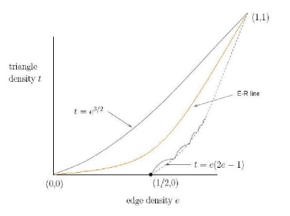
Figure 1: The set $R$ of all feasible edge-triangle homomorphism densities, defined in (2.10).

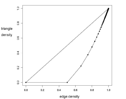
Figure 2: The set $P$ described in (2.11).

For a set $A\subset\mathbb{R}^{2}$, define $\mathrm{cone}(A)$ as the set of all conic combinations of points in $A$. It follows that the outer normals to the facets of $P$ are given by

$$\mathrm{cone}(o_{k}),\quad k=-1,0,1,\ldots,$$

i.e., by rays in $\mathbb{R}^{2}$ emanating from the origin and going along the direction of $o_{k}$. Finally, for $k=0,1,\ldots$ let $C_{k}=\mathrm{cone}(o_{k-1},o_{k})$ denote the normal cone to $P$ at $v_{k}$, i.e., a 2-dimensional pointed polyhedral cone spanned by $o_{k-1}$ and $o_{k}$. Denote by $C_{k}^{\circ}$ the topological interior of $C_{k}$. Then, since $P$ is bounded, for any non-zero $x\in\mathbb{R}^{2}$, there exists one $k$ for which either $x\in\mathrm{cone}(o_{k})$ or $x\in C_{k}^{\circ}$. The normal cones to the faces of $P$ form a locally finite polyhedral complex of cones, shown in Figure 3. As our results will demonstrate, each one of these cones uniquely identifies one of infinitely many asymptotic extremal behaviors of the edge-triangle model.

3 Variational analysis

In this section we characterize the extremal properties of $2$-parameter exponential random graphs and especially of the edge-triangle model using the variational approach described in Section 2.1. Chatterjee and Diaconis [10] showed that a typical graph drawn from a 2-parameter exponential random graph model with $H_{1}$ an edge and $H_{2}$ a fixed graph with chromatic number $\chi$ is a $(\chi-1)$-equipartite graph when $n$ is large, $\beta_{1}$ is fixed, and $\beta_{2}$ is large and negative, i.e., when the two parameters trace a vertical line downward.

In the hope of discovering other interesting extremal behaviors, we investigate the asymptotic structure of 2-parameter exponential random graph models along general straight lines. In particular, we will study sequences of model parameters of the form $\beta_{1}=a\beta_{2}+b$, where $a$ and $b$ are constants and $|\beta_{2}|\rightarrow\infty$. Thus, for any $\beta=(\beta_{1},\beta_{2})\in\mathbb{R}^{2}$, we can regard the quantities $\tilde{F}^{*}(\beta)$ and $\psi_{\infty}(\beta)$, defined in Section 2.1, as functions of $\beta_{2}$ only, and therefore will write them as $\tilde{F}^{*}(\beta_{2})$ and $\psi_{\infty}(\beta_{2})$ instead.

While we only give partial results for general exponential random graphs, we are able to provide a nearly complete characterization of the edge-triangle model. Even more refined results are possible, as will be shown in Section 4.

3.1 Asymptotic behavior of attractive $2$-parameter exponential random graph models along general lines

We will first consider the asymptotic behavior of “attractive” $2$-parameter exponential random graph models as $\beta_{2}\rightarrow\infty$. We will show that for $H_{1}$ an edge and $H_{2}$ any other finite simple graph, in the large $n$ limit, a typical graph drawn from the exponential model becomes complete under the topology induced by the cut distance if $a>-1$ or $a=-1$ and $b>0$; it becomes empty if $a<-1$ or $a=-1$ and $b<0$; while for $a=-1$ and $b=0$, it either looks like a complete graph or an empty graph. Below, for a non-negative constant $c$, we will write $u=c$ when $u$ is the constant graphon with value $c$.

Theorem 3.1.

Consider the 2-parameter exponential random graph model (1.2), with $H_{1}=K_{2}$ and $H_{2}$ a different, arbitrary graph. Let $\beta_{1}=a\beta_{2}+b$. Then

$$\lim_{\beta_{2}\rightarrow\infty}\sup_{\tilde{f}\in\tilde{F}^{*}(\beta_{2})}\delta_{\square}(\tilde{f},\tilde{U})=0,$$ (3.1)

where the set $U\subset\mathcal{W}$ is determined as follows:

• $U=\{1\}$ if $a>-1$ or $a=-1$ and $b>0$,

• $U=\{0,1\}$ if $a=-1$ and $b=0$, and

• $U=\{0\}$ if $a<-1$ or $a=-1$ and $b<0$.

When $a=-1$ and $b=0$, the limit points of the solution set of the variational problem (2.6) consist of two radically different graphons, one specifying an asymptotic edge density of $1$ and the other of $0$. This intriguing behavior was captured in [45], where it was shown that there is a continuous curve that asymptotically approaches the line $\beta_{1}=-\beta_{2}$, across which the graph transitions from being very sparse to very dense. Unfortunately, the variational technique used in the proof of the theorem does not seem to yield a way of deciding whether only one or both solutions can actually be realized. As we will see next, a similar issue arises when analyzing the asymptotic extremal behavior of the edge-triangle model along critical directions (see Theorem 3.3). In Section 4 we describe a different method of analysis that will allow us to resolve this rather subtle ambiguity within the edge-triangle model and reveal an asymptotic phase transition phenomenon. In particular, Theorem 4.4 there can be easily adapted to provide an analogous resolution of the case $a=-1$ and $b=0$ in Theorem 3.1.

We remark that, using same arguments, it is also possible to handle the case in which $\beta_{2}$ is fixed and $\beta_{1}$ diverges along horizontal lines. Then, we obtain the intuitively clear result that, in the large $n$ limit, a typical random graph drawn from this model becomes complete if $\beta_{1}\rightarrow\infty$, and empty if $\beta_{1}\rightarrow-\infty$. We omit the easy proof.

Figure 3: Cones, i.e., rays emanating from the origin, generated by the critical directions $o_{-1}$, $o_{0}$ and $o_{k}$, for $k=1,\ldots,40$. The plot also provides an accurate depiction of the locally finite polyhedral complex comprised by the normal cones to the faces of the set $P$ defined in (2.11).

The next two sections deal with the more challenging analysis of the asymptotic behavior of “repulsive” $2$-parameter exponential models as $\beta_{2}\rightarrow-\infty$. As mentioned earlier, the asymptotic properties of such models are largely unknown in this region.

3.2 Asymptotic behavior of repulsive $2$-parameter exponential random graph models along vertical lines

The purpose of this section is to give an alternate proof of Theorem 7.1 in [10] that uses classic results in extremal graph theory. In addition, this general result covers the asymptotic extremal behavior of the edge-triangle model along the vertical critical direction.

Recall that $\beta_{1}$ is fixed and we are interested in the asymptotics of $\tilde{F}^{*}(\beta_{2})$ and $\psi_{\infty}(\beta_{2})$ as $\beta_{2}\rightarrow-\infty$. We point out here that the limit process in $\beta_{2}$ may also be interpreted by taking $\beta_{1}=a\beta_{2}+b$ with $a=0$ and $b$ large negative. The importance of this latter interpretation will become clear in the next section. Our work here is inspired by related results of Fadnavis [18] and Radin and Sadun [44] in the case of $H_{2}$ being a triangle.

Theorem 3.2 (Chatterjee-Diaconis).

Consider the 2-parameter exponential random graph model (1.2), with $H_{1}=K_{2}$ and $H_{2}$ a different, arbitrary graph. Fix $\beta_{1}$. Let $r=\chi(H_{2})$ be the chromatic number of $H_{2}$. Let $p=e^{2\beta_{1}}/(1+e^{2\beta_{1}})$. Then

$$\lim_{\beta_{2}\rightarrow-\infty}\sup_{\tilde{f}\in\tilde{F}^{*}(\beta_{2})}\delta_{\square}(\tilde{f},\tilde{U})=0,$$ (3.2)

where the set $U\subset\mathcal{W}$ is given by $U=\{pf^{K_{r-1}}\}$ (see (2.12)).

As explained in [10], the above result can be interpreted as follows: if $\beta_{2}$ is negative and large in magnitude and $n$ is big, then a typical graph $G_{n}$ drawn from the 2-parameter exponential model (1.2) looks roughly like a complete $(\chi(H_{2})-1)$-equipartite graph with $1-p$ fraction of edges randomly deleted, where $p=e^{2\beta_{1}}/(1+e^{2\beta_{1}})$.

3.3 Asymptotic quantization of edge-triangle model along general lines

In this section we conduct a thorough analysis of the asymptotic behavior of the edge-triangle model as $\beta_{2}\rightarrow-\infty$. As usual, we take $\beta_{1}=a\beta_{2}+b$, where $a$ and $b$ are fixed constants. The $a=0$ situation is a special case of what has been discussed in the previous section: If $n$ is large, then a typical graph $G_{n}$ drawn from the edge-triangle model looks roughly like a complete bipartite graph with $1/(1+e^{2b})$ fraction of edges randomly deleted. It is not too difficult to establish that if $a>0$, then independent of $b$, a typical graph $G_{n}$ becomes empty in the large $n$ limit. Intuitively, this should be clear: $\beta_{1}$ and $\beta_{2}$ both large and negative entail that $G_{n}$ would have minimal edge and triangle densities. However, the case $a<0$ leads to an array of non-trivial and intriguing extremal behaviors for the edge-triangle model, and they are described in our next result. We emphasize that our analysis relies on the explicit characterization by Razborov [46] of the lower boundary of the set $R$ of (the closure of) all edge and triangle density homomorphisms (see (2.14)) and on the fact that the extreme points of $P$ are the points $\{v_{k},k=0,1,\ldots\}$, given in (2.13). Recall that these points correspond to the density homomorphisms of the Turán graphons $f^{K_{k+1}}$, $k=0,1,\ldots$, as shown in (2.12).

Theorem 3.3.

Consider the edge-triangle exponential random graph model (2.7). Let $\beta_{1}=a\beta_{2}+b$ with $a<0$ and, for $k\geq 0$, let $a_{k}=-\frac{k(3k+5)}{(k+1)(k+2)}$. Then,

$$\lim_{\beta_{2}\rightarrow-\infty}\sup_{\tilde{f}\in\tilde{F}^{*}(\beta_{2})}\delta_{\square}(\tilde{f},\tilde{U})=0,$$ (3.3)

where the set $U\subset\mathcal{W}$ is determined as follows:

• $U=\{f^{K_{k+2}}\}$ if $a_{k}>a>a_{k+1}$ or $a=a_{k}$ and $b>0$,

• $U=\{f^{K_{k+1}},f^{K_{k+2}}\}$ if $a=a_{k}$ and $b=0$, and

• $U=\{f^{K_{k+1}}\}$ if $a=a_{k}$ and $b<0$.

Remark.

Notice that the case $a=a_{k}$ and $b=0$ corresponds to the critical direction $o_{k}$, for $k=1,2,\ldots$.

The above result says that, if $\beta_{1}=a\beta_{2}+b$ with $a<0$ and $\beta_{2}$ large negative, then in the large $n$ limit, any graph drawn from the edge-triangle model is indistinguishable in the cut metric topology from a complete $(k+2)$-equipartite graph if $a_{k}>a>a_{k+1}$ or $a=a_{k}$ and $b>0$; it looks like a complete $(k+1)$-equipartite graph if $a=a_{k}$ and $b<0$; and for $a=a_{k}$ and $b=0$, it either behaves like a complete $(k+1)$-equipartite graph or a complete $(k+2)$-equipartite graph. Lastly it becomes complete if $a\leq\lim_{k\rightarrow\infty}a_{k}=-3$. Overall, these results describe in a precise manner the array of all possible asymptotic extremal behaviors of the edge-triangle model, and link them directly to the geometry of the natural parameter space as captured by the polyhedral complex of cones shown in Figure 3.

When $a=a_{k}$ and $b=0$, for any $k=0,1,\ldots$, i.e., when the parameters diverge along the critical direction $o_{k}$, Theorem 3.3 suffers from the same ambiguity as Theorem 3.1: the limit points of the solution set of the variational problem (2.3) as $\beta_{2}\rightarrow-\infty$ are Turán graphons with $k+1$ and $k+2$ classes. Though already quite informative, this result remains somewhat unsatisfactory because it does not indicate whether both such graphons are actually realizable in the limit and in what manner. As we remarked in the discussion following Theorem 3.1, our method of proof, largely based on and inspired by the results in [10], does not seem to suggest a way of clarifying this issue. In the next section we will present a completely different asymptotic analysis yielding different types of convergence guarantees. As in the present section, two limit processes will be considered: the network size $n$ grows unbounded and the natural parameters $\beta$ diverge, with the order of limits interchanged. The two approaches in Sections 3 and 4 produce similar results except along critical directions, where the second approach has the added power of resolving the aforementioned ambiguities.

3.4 Probabilistic convergence of sequences of graphs from edge-triangle model

The results obtained in Sections 3.1, 3.2 and 3.3 characterize the extremal asymptotic behavior of the edge-triangle model through functional convergence in the cut topology within the space $\widetilde{\mathcal{W}}$. Our explanation of such results though has more of a probabilistic flavor. Here we briefly show how this interpretation is justified. By combining (2.5), established in Theorem 3.2 of [10], with the theorems in Sections 3.1, 3.2 and 3.3, and a standard diagonal argument, we can deduce the existence of subsequences of the form $\{(n_{i},\beta_{2,i})\}_{i=1,2\ldots}$, where $n_{i}\rightarrow\infty$ and $\beta_{2,i}\rightarrow\infty$ or $-\infty$ as $i\rightarrow\infty$, such that the following holds. For fixed $a$ and $b$, let $\{G_{i}\}_{i=1,2,\ldots}$ be a sequence of random graphs drawn from the sequence of edge-triangle models with node sizes $\{n_{i}\}$ and parameter values $\{(a\beta_{2,i}+b,\beta_{2,i})\}$. Then

$$\delta_{\square}(\tilde{f}^{G_{i}},\tilde{U})\rightarrow 0\hbox{ in probability as }i\rightarrow\infty,$$

where the set $U\subset\mathcal{W}$, which depends on $a$ and $b$, is described in Theorems 3.1, 3.2 and 3.3. In Section 4.5 we will obtain a very similar result by entirely different means.

4 Finite $n$ analysis

In the remainder part of this paper we will present an alternative analysis of the asymptotic behavior of the edge-triangle model using directly the properties of the exponential families and their closure in the finite $n$ case instead of the variational approach of [10, 44, 45]. Though the results in this section are seemingly similar to the ones in Section 3, we point out that there are marked differences. First, while in Section 3 we study convergence in the cut metric for the quotient space $\widetilde{\mathcal{W}}$, here we are concerned instead with convergence in total variation of the edge and triangle homomorphism densities. Secondly, the double asymptotics, in $n$ and in the magnitude of $\beta$, are not the same. In Section 3, the system size $n$ goes to infinity first followed by the divergence of the parameter $\beta_{2}$ to positive or negative infinity. In contrast, here we first let the magnitude of the natural parameter $\beta$ diverge to infinity so as to isolate a simpler “restricted” edge-triangle sub-model, and then study its limiting properties as $n$ grows. Though both approaches are in fact asymptotic, we characterize the latter as “finite $n$”, to highlight the fact that we are not working with a limiting system and because, even with finite $n$, the extremal properties already begin to emerge. Despite these differences, the conclusions we can derive from both types of analysis are rather similar. Furthermore, they imply a nearly identical convergence in probability in the cut topology (see Sections 3.4 and 4.5).

Besides giving a rather strong form of asymptotic convergence, one of the appeals of the finite $n$ analysis consists in its ability to provide a more detailed categorization of the limiting behavior of the model along critical directions using simple geometric arguments based on the dual geometry of $P$, the convex hull of edge-triangle homomorphism densities. Specifically, we will demonstrate that, asymptotically, the edge-triangle model undergoes phase transitions along critical directions, where its homomorphism densities will converge in total variation to the densities of one of two Turán graphons, both of which are realizable. In addition we are able to state precise conditions on the natural parameters for such transitions to occur.

4.1 Exponential families

We begin by reviewing some of the standard theory of exponential families and their closure in the context of the edge-triangle model. We refer the readers to Barndorff-Nielsen [2] and Brown [9] for exhaustive treatments of exponential families, and to Csiszár and Matúš [12, 13], Geyer [23], and Rinaldo et al. [47] for specialized results on the closure of exponential families directly relevant to our problem.

Recall that we are interested in the exponential family of probability distributions on $\mathcal{G}_{n}$ such that, for a given choice of the natural parameters $\beta\in\mathbb{R}^{2}$, the probability of observing a network $G_{n}\in\mathcal{G}_{n}$ is

$$\mathbb{P}_{n,\beta}(G_{n})=\exp\left(n^{2}\left(\langle\beta,t(G_{n})\rangle-\psi_{n}(\beta)\right)\right),\quad\beta\in\mathbb{R}^{2},$$ (4.1)

where $\psi_{n}(\beta)$ is the normalizing constant and the function $t(\cdot)$ is given in (2.8). We remark that the above model assigns the same probability to all graphs in $\mathcal{G}_{n}$ that have the same image under $t(\cdot)$. We let $S_{n}=\{t(G_{n}),G_{n}\in\mathcal{G}_{n}\}\subset[0,1]^{2}$ be the set of all possible vectors of densities of graph homomorphisms of $K_{2}$ and $K_{3}$ over the set $\mathcal{G}_{n}$ of all simple graphs on $n$ nodes (see (2.8)). By (4.1), the family on $\mathcal{G}_{n}$ will induce the exponential family of probability distributions $\mathcal{E}_{n}=\{\mathbb{P}_{n,\beta},\beta\in\mathbb{R}^{2}\}$ on $S_{n}$, such that the probability of observing a point $x\in S_{n}$ is

$$\mathbb{P}_{n,\beta}(x)=\exp\left(n^{2}\left(\langle\beta,x\rangle-\psi_{n}(\beta)\right)\right)\nu_{n}(x),\quad\beta\in\mathbb{R}^{2},$$ (4.2)

where $\nu_{n}(x)=|\{t^{-1}(x)\}|$ is the measure on $S_{n}$ induced by the counting measure on $\mathcal{G}_{n}$ and $t(\cdot)$. For each $n$, the family $\mathcal{E}_{n}$ has finite support not contained in any lower dimensional set (see Lemma 4.1 below) and, therefore, is full and regular and, in particular, steep.

We will study the limiting behavior of sequences of models of the form $\{\mathbb{P}_{n,\beta+ro}\}$, where $\beta$ and $o$ are fixed vectors in $\mathbb{R}^{2}$ and $n$ and $r$ are parameters both tending to infinity. While it may be tempting to regard $n$ as a surrogate for an increasing sample size, this would in fact be incorrect. Models parametrized by different values of $n$ and the same $r$ cannot be embedded (for the edge-triangle model) in any sequence of consistent probability measures, since the probability distribution corresponding to the smaller network cannot in general be obtained from the other by marginalization, for a fixed choice of $\beta$. See [50] for details. We will show that different choices of the direction $o$ will yield different extremal behaviors of the model and we will categorize the variety of these behaviors as a function of $o$ and, whenever it matters, of $\beta$. A key feature of our analysis is the direct link to the geometric properties of the polyhedral complex $\{C_{k},k=-1,0,\ldots\}$ defined by the set $P$ (see Section 2.2).

Overall, the results of this section are obtained with non-trivial extensions of techniques described in the exponential families literature. Indeed, for fixed $n$, determining the limiting behaviors of the family $\mathcal{E}_{n}$ along sequences of natural parameters $\{\beta+ro\}_{r\rightarrow\infty}$ for each unit norm vector $o$ and each $\beta$ is the main technical ingredient in computing the total variation closure of $\mathcal{E}_{n}$. In particular Geyer [23] refers to the directions $o$ as the “directions of recession” of the model. The relevance of the directions of recession to the asymptotic behavior of exponential random graphs is now well known, as demonstrated in the work of Handcock [28] and Rinaldo et al. [47].

4.2 Finite $n$ geometry

As we saw in Section 3, the critical directions are determined by the limiting object $P$. For finite $n$, an analogous role is played by the convex support of $\mathcal{E}_{n}$, which is given by the polytope

$$P_{n}=\mathrm{convhull}(S_{n})\subset[0,1]^{2}.$$

The interior of $P_{n}$ is equal to all possible expected values of the sufficient statistics $\{\mathbb{E}_{n,\beta}\left(t(G_{n})\right),\beta\in\mathbb{R}^{2}\}$, where $\mathbb{E}_{n,\beta}$ is the expectation operator with respect to the measure $\mathbb{P}_{n,\beta}$. Thus, it provides a different parametrization of $\mathcal{E}_{n}$, known as the mean-value parametrization (see, e.g., [2, 9]). Unlike the natural parametrization, the mean value parametrization has explicit geometric properties that turn out to be particularly convenient in order to describe the closure of $\mathcal{E}_{n}$, and, ultimately, the asymptotics of the model.

The next lemma characterizes the geometric properties of $P_{n}$. The most significant of these properties is that $\lim_{n}P_{n}=P$, an easy result that turns out to be the key for our analysis. Recall that we denote by $T(n,r)$ any Turán graph on $n$ nodes with $r$ classes. For $k=0,1,\ldots,n-1$, set $v_{k,n}=t(T(n,k+1))$ and let $L_{k,n}$ denote the line segment joining $v_{k,n}$ and $v_{k+1,n}$.

Lemma 4.1.

1. The polytope $P_{n}$ is spanned by the points $\{v_{k,n},k=0,1,\ldots,\lceil n/2\rceil-1\}$ and $v_{n-1,n}$.

2. $\lim_{n}P_{n}=P$.

3. If $n$ is a multiple of $(k+1)(k+2)$, then $v_{k,n}=v_{k}$ and $v_{k+1,n}=v_{k+1}$. In addition, for all such $n$, $L_{k,n}\cap S_{n}=\{v_{k},v_{k+1}\}$.

Part 2. of Lemma 4.1 implies that for each $k$, $\lim_{n}v_{k,n}=v_{k}$, a fact that will be used in Theorem 4.2 to describe the asymptotics of the model along generic (i.e., non-critical directions). This conclusion still holds if the polytopes $P_{n}$ are the convex hulls of isomorphism, not homomorphism, densities. In this case, however, we have that $P_{n}\supset P$ for each $n$ (see [16]). The seemingly inconsequential fact stated in part 3. is instead of technical significance for our analysis of the phase transitions along critical directions, as will be described in Theorem 4.3. We take note that when $n$ is not a multiple of $(k+1)(k+2)$, part 3. does not hold in general.

4.3 Asymptotics along generic directions

Our first result, which gives similar finding as in Section 3.3 shows that, for large $n$, if the distribution is parametrized by a vector with very large norm, then almost all of its mass will concentrate on the isomorphic class of a Turán graph (possibly the empty or the complete graph). Which Turán graph it concentrates on will essentially depend on the “direction” of the parameter vector with respect to the origin. Furthermore, there is an array of extremal directions that will give the same isomorphic class of a Turán graph.

Theorem 4.2.

Let $o$ and $\beta$ be vectors in $\mathbb{R}^{2}$ such that $o\neq o_{k}$ for $k=-1,0,1,\ldots$ and let $k$ be such that $o\in C_{k}^{\circ}$. For any $0<\epsilon<1$ arbitrarily small, there exists an $n_{0}=n_{0}(\beta,\epsilon,o)>0$ such that the following holds: for every $n>n_{0}$, there exists an $r_{0}=r_{0}(\beta,\epsilon,o,n)>0$ such that for all $r>r_{0}$,

$$\mathbb{P}_{n,\beta+ro}(v_{k,n})>1-\epsilon.$$

Remark.

If in the theorem above we consider only values of $n$ that are multiples of $(k+1)(k+2)$ then, by Lemma 4.1, $v_{k,n}=v_{k}$ for all such $n$, which implies convergence in total variation to the point mass at $v_{k}$.

The theorem shows that any choice of $o\in C_{k}^{\circ}$ will yield the same asymptotic (in $n$ and $r$) behavior, captured by the Turán graphon with $k+1$ classes. This can be further strengthened to show that the convergence is uniform in $o$ over compact subsets of $C_{k}^{\circ}$. See [47] for details. Interestingly, the initial value of $\beta$ does not play any role in determining the asymptotics of $\mathbb{P}_{n,\beta+ro}$, which instead depends solely on which cone $C_{k}$ contains in its interior the direction $o$. Altogether, Theorem 4.2 can be interpreted as follows: the interiors of the cones of the infinite polyhedral complex $\{C_{k},k=-1,0,1,\ldots\}$ represent equivalence classes of “extremal directions” of the model, whereby directions in the same class will parametrize, for large $n$ and $r$, the same degenerate distribution on some Turán graph.

4.4 Asymptotics along critical directions

Theorem 4.2 provides a complete categorization of the asymptotics (in $n$ and $r$) of probability distributions of the form $P_{n,\beta+ro}$ for any generic direction $o$ other than the critical directions $\{o_{k},k=-1,0,1,\ldots\}$. We now consider the more delicate cases in which $o=o_{k}$ for some $k$. Recall that, according to Theorem 3.3, in these instances the typical graph drawn from the model will converge (as $n$ and $r$ grow and in the cut metric) to a large Turán graph, whose number of classes is not entirely specified.

Our first result characterizes such behavior along subsequences of the form $n=j(k+1)(k+2)$, for $j=1,2,\ldots$ and $k$ a positive integer. Interestingly, and in contrast with Theorem 4.2, the limiting behavior along any critical direction $o_{k}$ depends on $\beta$ in a discontinuous manner. Before stating the result we will need to introduce some additional notation. Let $l_{k}\in\mathbb{R}^{2}$ be the unit norm vector spanning the one-dimensional linear subspace $\mathcal{L}_{k}$ given by the line through the origin parallel to $L_{k}$, where $k>0$, so $l_{k}$ is just a rescaling of the vector

$$\left(1,\frac{k(3k+5)}{(k+1)(k+2)}\right).$$

Next let $H_{k}=\{x\in\mathbb{R}^{2}\colon\langle x,l_{k}\rangle=0\}=\mathcal{L}_{k}^{\bot}$ be the line through the origin defining the linear subspace orthogonal to $\mathcal{L}_{k}$ and let

$$H^{+}_{k}=\{x\in\mathbb{R}^{2}\colon\langle x,l_{k}\rangle>0\}\quad\text{and}\quad H^{-}_{k}=\{x\in\mathbb{R}^{2}\colon\langle x,l_{k}\rangle<0\}$$ (4.3)

be the positive and negative half-spaces cut out by $H_{k}$, respectively. Notice that the linear subspace $\mathcal{L}^{\bot}_{k}$ is spanned by the vector $o_{k}$ defined in (2.15).

We will make the simplifying assumption that $n$ is a multiple of $(k+1)(k+2)$. This implies, in particular, that $v_{k,n}=v_{k}$ and $v_{k+1,n}=v_{k+1}$ are both vertices of $P_{n}$ and that the line segment $L_{k,n}=L_{k}$ is a facet of $P_{n}$ whose normal cone is spanned by the point $o_{k}$.

Theorem 4.3.

Let $k$ be a positive integer, $\beta\in\mathbb{R}^{2}$ and $0<\epsilon<1$ be arbitrarily small. Then there exists an $n_{0}=n_{0}(\beta,\epsilon,k)>0$ such that the following holds: for every $n>n_{0}$ and a multiple of $(k+1)(k+2)$ there exists an $r_{0}=r_{0}(\beta,\epsilon,k,n)>0$ such that for all $r>r_{0}$,

• if $\beta\in H^{+}_{k}$ or $\beta\in H_{k}$ then $\mathbb{P}_{n,\beta+ro_{k}}(v_{k+1})>1-\epsilon$,

• if $\beta\in H^{-}_{k}$ then $\mathbb{P}_{n,\beta+ro_{k}}(v_{k})>1-\epsilon$.

The previous result shows that, for large values of $r$ and $n$ (assumed to be a multiple of $(k+1)(k+2)$), the probability distribution $P_{n,\beta+ro_{k}}$ will be concentrated almost entirely on either $v_{k}$ or $v_{k+1}$, depending on which side of $H_{k}$ the vector $\beta$ lies. In particular, the actual value of $\beta$ does not play any role in the asymptotics: only its position relative to $H_{k}$ matters. An interesting consequence of our result is the discontinuity of the natural parametrization along the line $H_{k}$ in the limit as both $n$ and $r$ tend to infinity. This is in stark contrast to the limiting behavior of the same model when $n$ is infinity and $r$ tends to infinity: in this case the natural parametrization is a smooth (though non-minimal) parametrization.

We now consider the critical directions $o_{-1}$ and $o_{0}$ (see (2.15)), which are not covered by Theorem 4.3. We will first describe the behavior of $\mathcal{E}_{n}$ along the direction of recession $o_{-1,n}:=\left(-1,\frac{n}{n-2}\right)$. This is the outer normal to the segment joining the vertices $v_{0,n}=(0,0)$ and $v_{n-1,n}=\left(1-\frac{1}{n},\left(1-\frac{1}{n}\right)\left(1-\frac{2}{n}\right)\right)$ of $P_{n}$, representing the empty and the complete graph, respectively. Notice that $o_{-1,n}\rightarrow o_{-1}$ as $n\rightarrow\infty$. In this case, we show that, for $n$ and $r$ large, the probability $P_{n,\beta+ro_{n}}$, with $\beta=(\beta_{1},\beta_{2})$, assigns almost all of its mass to the empty graph when $\beta_{1}+\beta_{2}<0$ and to the complete graph when $\beta_{1}+\beta_{2}>0$, and it is uniform over $v_{0,n}$ and $v_{n-1,n}$ when $\beta_{1}n(n-1)+\beta_{2}(n-1)(n-2)=0$.

Theorem 4.4.

Let $\beta=(\beta_{1},\beta_{2})\in\mathbb{R}^{2}$ be a fixed vector and $0<\epsilon<1$ be arbitrarily small. Then for every $n$ there exists an $r_{0}=r_{0}(\beta,\epsilon,n)$ such that, for all $r>r_{0}$, the total variation distance between $P_{n,\beta+ro_{n}}$ and the probability distribution which assigns to the points $v_{0,n}$ and $v_{n-1,n}$ the probabilities

$$\frac{1}{1+\exp\big{(}\beta_{1}n(n-1)+\beta_{2}(n-1)(n-2)\big{)}}\$$

and

$$\frac{\exp\big{(}\beta_{1}n(n-1)+\beta_{2}(n-1)(n-2)\big{)}}{1+\exp\big{(}\beta_{1}n(n-1)+\beta_{2}(n-1)(n-2)\big{)}},$$

respectively, is less than $\epsilon$.

In the last result of this section we will turn to the critical direction $o_{0}=\left(0,-1\right)$, which, for every $n\geq 2$, is the outer normal to the horizontal facet of $P_{n}$ joining the points $(0,0)$ and

$$v_{1,n}=\left(\frac{2\lceil n/2\rceil(n-\lceil n/2\rceil)}{n^{2}},0\right),$$

which we denote with $L_{0,n}$. Let $\mathcal{G}_{n,0}$ denote the subset of $\mathcal{G}_{n}$ consisting of triangle free graphs. For each $n$, consider the exponential family $\{\mathbb{Q}_{n,\beta_{1}},\beta_{1}\in\mathbb{R}\}$ of probability distributions on $L_{0,n}\cap S_{n}$ given by

$$\mathbb{Q}_{n,\beta_{1}}(x)=\exp\left(n^{2}\left(\beta_{1}x_{1}-\phi_{n}(\beta_{1})\right)\right)\nu_{n}(x),\quad x\in L_{n,0}\cap S_{n},\,\,\beta_{1}\in\mathbb{R},$$ (4.4)

where $\phi_{n}(\beta_{1})$ is the normalizing constant and $\nu_{n}(x)=|\{t^{-1}(x)\}|$ is the measure on $L_{0,n}$ induced by the counting measure on $\mathcal{G}_{n,0}$ and $t(\cdot)$.

Theorem 4.5.

Let $\beta=(\beta_{1},\beta_{2})\in\mathbb{R}^{2}$ be a fixed vector and $0<\epsilon<1$ an arbitrary number. Then for every $n$ there exists an $r_{0}=r_{0}(\beta,\epsilon,n)$ such that for all $r>r_{0}$ the total variation distance between $\mathbb{P}_{n,\beta+ro_{0}}$ and $\mathbb{Q}_{n,\beta_{1}}$ is less than $\epsilon$.

When compared to Theorem 3.2, Theorem 4.5 is less informative, as the class of triangle free graphs is larger than the class of subgraphs of the Turán graphs $T(n,2)$. We conjecture that this gap can indeed be resolved by showing that, for each $\beta_{1}$, $\mathbb{Q}_{n,\beta_{1}}$ assigns a vanishingly small mass to the set of all triangle free graphs that are not subgraphs of some $T(n,2)$ as $n\rightarrow\infty$. See [17] for relevant results.

4.5 From convergence in total variation to stochastic convergence in cut distance

The results presented so far in Section 4 concern convergence in total variation of the homomorphism densities of edges and triangles to point mass distributions at points $v_{k,n}$. They describe a rather different type of asymptotic guarantees from the one obtained in Section 3, whereby convergence occurs in the functional space $\widetilde{\mathcal{W}}$ under the cut metric. Nonetheless, both sets of results are qualitatively similar and lend themselves to nearly identical interpretations. Here we sketch how the total variation convergence results imply convergence in probability in the cut metric along subsequences. Notice that this is precisely the same type of conclusions we obtained at the end of the variational analysis, as remarked in Section 3.4.

We will let $n$ be of the form $j(k+1)(k+2)$ for $j=1,2,\ldots$. For simplicity we consider a direction $o$ in the interior of $C_{k}$, for some $k$. By Theorem 4.2 and using a standard diagonal argument, there exists a subsequence $\{(n_{i},r_{i})\}_{i=1,2,\ldots}$ such that the sequence of probability measures $\{\mathbb{P}_{n_{i},\beta+r_{i}o}\}_{i=1,2,\ldots}$ converges in total variation to the point mass at $v_{k}$. Thus, for each $\epsilon>0$, there exists an $i_{0}=i_{0}(\epsilon)$ such that, for all $i>i_{0}$, the probability that a random graph $G_{n_{i}}$ drawn from the probability distribution $\mathbb{P}_{n_{i},\beta+r_{i}o}$ is such that $t(G_{i})\neq v_{k}$ is less than $\epsilon$. Let $\mathcal{A}_{i}$ be the event that $t(G_{i})=v_{k}$ and for notational convenience denote $\mathbb{P}_{n_{i},\beta+r_{i}o}$ by $\mathbb{P}_{i}$. Thus, for each $i>i_{0}$, $\mathbb{P}_{i}(\mathcal{A}_{i})>1-\epsilon$. Let $H$ be any finite graph. Then, denoting with $\mathbb{E}_{i}$ the expectation with respect to $\mathbb{P}_{i}$ and with $1_{\mathcal{A}_{i}}$ the indicator function of $\mathcal{A}_{i}$, we have

$$\mathbb{E}_{i}[t(H,G_{i})]=\mathbb{E}_{i}[t(H,G_{i})1_{\mathcal{A}_{i}}]+\mathbb{E}_{i}[t(H,G_{i})1_{\mathcal{A}^{c}_{i}}],$$

where

$$\mathbb{E}_{i}[t(H,G_{i})1_{\mathcal{A}_{i}}]=t(H,T(n_{i},k+1))=t(H,f^{K_{k+1}}),$$

since, given our assumption on the $n_{i}$’s, the point in $\widetilde{\mathcal{W}}$ corresponding to $T(n_{i},k+1)$ is $\tilde{f}^{K_{k+1}}$ for all $i$. Thus, using the fact that density homomorphisms are bounded by $1$,

$$\mathbb{E}_{i}[t(H,G_{i})]-t(H,f^{K_{k+1}})=\mathbb{E}_{i}[t(H,G_{i})1_{\mathcal{A}^{c}_{i}}]\leq\mathbb{P}_{i}(\mathcal{A}^{c}_{i})=\epsilon$$

for all $i>i_{0}$. Thus, we conclude that $\lim_{i}\mathbb{E}_{i}[t(H,G_{i})]=t(H,f^{K_{k+1}})$ for each finite graph $H$. By Corollary 3.2 in [14], as $i\rightarrow\infty$,

$$\delta_{\square}(\tilde{f}^{G_{i}},\tilde{f}^{K_{k+1}})\rightarrow 0\quad\text{in probability.}$$

Similar arguments apply to the case in which $o=o_{k}$ for some $k>0$. Using instead Theorem 4.3, we obtain that, if $\{G_{n_{i}}\}_{i=1,2\ldots}$ is a sequence of random graphs drawn from the sequence of probability distributions $\{\mathbb{P}_{n_{i},\beta+r_{i}o}\}$, then, as $i\rightarrow\infty$,

$$\delta_{\square}(\tilde{f}^{G_{i}},\tilde{f}^{K_{k+2}})\rightarrow 0\quad\text{if }\beta\in H^{+}_{k}\text{ or }\beta\in H_{k},$$

and

$$\delta_{\square}(\tilde{f}^{G_{i}},\tilde{f}^{K_{k+1}})\rightarrow 0\quad\text{if }\beta\in H^{-}_{k}$$

in probability.

5 Illustrative figures

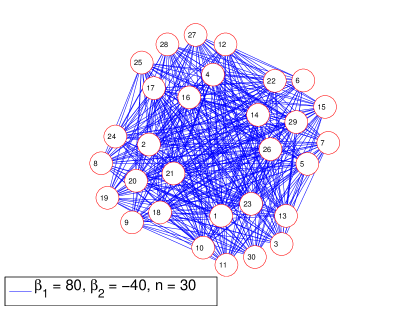
Figure 4: A simulated realization of the exponential random graph model on $30$ nodes with edges and triangles as sufficient statistics, where the initial value $\beta=(0,0)$, $r=80$, and the generic direction $o=(1,-1/2)$ in $C_{3}^{o}$. The structure of the simulated graph matches the predictions of Theorem 4.2.

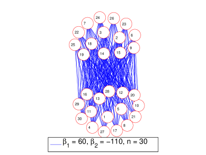
Figure 5: A simulated realization of the exponential random graph model on $30$ nodes with edges and triangles as sufficient statistics, where the initial value $\beta=(20,-80)$ in $H_{1}^{-}$, $r=40$, and the critical direction $o_{1}=(1,-3/4)$. The structure of the simulated graph matches the predictions of Theorem 4.3.

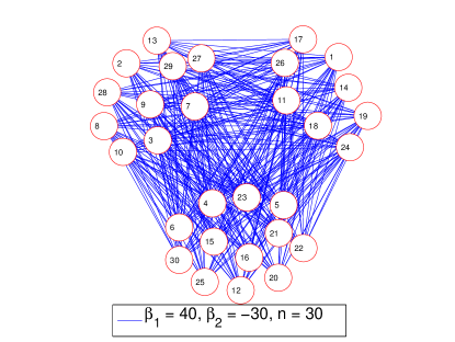
Figure 6: A simulated realization of the exponential random graph model on $30$ nodes with edges and triangles as sufficient statistics, where the initial value $\beta=(0,0)$ in $H_{1}$, $r=40$, and the critical direction $o_{1}=(1,-3/4)$. The structure of the simulated graph matches the predictions of Theorem 4.3.

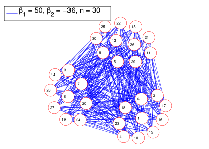
Figure 7: A simulated realization of the exponential random graph model on $30$ nodes with edges and triangles as sufficient statistics, where the initial value $\beta=(10,-6)$ in $H_{1}^{+}$, $r=40$, and the critical direction $o_{1}=(1,-3/4)$. The structure of the simulated graph matches the predictions of Theorem 4.3.

We have validated our theoretical findings with simulations of the edge-triangle model under various specifications on the model parameters. Figure 4 depicts a typical realization from the model when $n=30$ and $o$ is in $C_{3}^{\circ}$. As predicted by Theorem 4.2, the resulting graph is complete equipartite with $4$ classes. Figures 5, 6 and 7 exemplify the results of Theorem 4.3. For these simulations, we consider the critical direction $o_{1}=(1,-3/4)$ and again a network size of $n=30$, and then vary the initial values of $\beta$. Figures 5 and 7 show respectively the outcome of two typical draws when $\beta$ is in $H_{1}^{-}$ and $H_{1}^{+}$, respectively. As predicted by our theorem, we obtain a complete bipartite and tripartite graph. Figure 6 depicts instead the case of $\beta$ exactly along the hyperplane $H_{1}$, for which, according to our theory, a typical realization would again be a complete tripartite graph.

As a final remark, simulating from the extremal parameter configurations we described using off-the-shelf MCMC methods (see, e.g., [24, 31] and, for a convergence result, [10]) is quite difficult. This is due to the fact that under these extremal settings, the model places most of its mass on only one or two types of Turán graphs, and the chance of a chain being able to explore adequately the space of graphs using local moves and to eventually reach the configuration of highest energy is essentially minuscule.

6 Further discussions

As shown by Bhamidi et al. [3] and Chatterjee and Diaconis [10], as $n\rightarrow\infty$, when $\beta_{2}$ is positive, a typical graph drawn from the standard edge-triangle exponential random graph model (2.7) has a somewhat trivial structure: it always looks like an Erdős-Rényi random graph or a mixture of Erdős-Rényi random graphs. By raising the triangle density to an exponent $\gamma>0$, Lubetzky and Zhao [39] proposed a natural generalization:

$$\mathbb{P}_{n,\beta}(G_{n})=\exp\left(n^{2}(\beta_{1}t(K_{2},G_{n})+\beta_{2}t(K_{3},G_{n})^{\gamma}-\psi_{n}(\beta))\right),$$ (6.1)

which enabled the model to exhibit a non-trivial structure even when $\beta_{2}$ is positive. This generalized model still features the Erdős-Rényi behavior if $\gamma\geq 2/3$; but for $\gamma<2/3$, there exist regions of values of $(\beta_{1},\beta_{2})$ for which a typical graph drawn from the model has symmetry breaking. We are interested to know how the double asymptotic framework discussed in the earlier sections would lend itself to this generalized model.

Below we adapt our first main result for the standard model (Theorem 3.1) to the generalized model and carry out some explicit calculations. As we will see, it conforms to the findings in [39] and gives the limiting graphon structure for the solution of the variational problem. The proof of the theorem offers one explanation for why $2/3$ is a separating value for the exponent $\gamma$: it is intimately tied to the upper boundary of the feasible edge-triangle homomorphism densities. Furthermore, the theorem provides convincing evidence that the region of symmetry breaking for the generalized edge-triangle model is potentially much larger than the ones depicted on page 5 of [39]. We remark that, using similar arguments, it is also possible to adapt our other results for the standard model to the generalized model, but the calculations would be rather involved, especially when they concern the lower boundary of the feasible edge-triangle homomorphism densities. Recall that for a non-negative constant $c$, we write $u=c$ when $u$ is the constant graphon with value $c$.

Theorem 6.1.

Consider the generalized edge-triangle exponential random graph model (6.1). Let $\beta_{1}=a\beta_{2}+b$. Then

$$\lim_{\beta_{2}\rightarrow\infty}\sup_{\tilde{f}\in\tilde{F}^{*}(\beta_{2})}\delta_{\square}(\tilde{f},\tilde{U})=0,$$ (6.2)

where for $\gamma\geq 2/3$, the set $U\subset\mathcal{W}$ is determined as follows:

• $U=\{1\}$ if $a>-1$ or $a=-1$ and $b>0$,

• $U=\{0,1\}$ if $a=-1$ and $b=0$, and

• $U=\{0\}$ if $a<-1$ or $a=-1$ and $b<0$;

and for $\gamma<2/3$, the set $U\subset\mathcal{W}$ is determined as follows:

• $U=\{1\}$ if $a\geq-\frac{3}{2}\gamma$, and

• $U=\{f\}$ if $a<-\frac{3}{2}\gamma$,

where $f(x,y)=\left\{\begin{array}[]{ll}1&\hbox{if $0\leq x,y\leq\left(-\frac{2a}{3\gamma}\right)^{\frac{1}{3\gamma-2}}$,}\\ 0&\hbox{otherwise.}\\ \end{array}\right.$

7 Proofs

Proof of Theorem 3.1.

Suppose $H_{2}$ has $p$ edges. Subject to $\beta_{1}=a\beta_{2}+b$, the variational problem (2.6) in the Erdős-Rényi region takes the following form: Find $u$ so that

$$\beta_{2}(au+u^{p})+bu-I(u)$$ (7.1)

is maximized. Take an arbitrary sequence $\beta_{2}^{(i)}\rightarrow\infty$. Let $u_{i}$ be a maximizer corresponding to $\beta_{2}^{(i)}$ and $u^{*}$ be a limit point of the sequence $\{u_{i}\}$. By the boundedness of $bu$ and $I(u)$, we see that $u^{*}$ must maximize $au+u^{p}$. For $a\neq-1$, this maximizer is unique, but for $a=-1$, both $0$ and $1$ are maximizers. In this case, $\beta_{2}(au+u^{p})=0$, so we check the value of $bu-I(u)$ as well. We conclude that $u^{*}=1$ for $b>0$, $u^{*}=0$ for $b<0$, and $u^{*}$ may be either $1$ or $0$ for $b=0$. ∎

The following lemma appeared as an exercise in [36].

Lemma 7.1 (Lovász).

Let $F$ and $G$ be two simple graphs. Let $f$ be a graphon such that $t(F,G)>0$ and $t(G,f)>0$. Then $t(F,f)>0$.

Proof.

Suppose $|V(F)|=m$ and $|V(G)|=n$. Since $t(G,f)>0$, there is a Lebesgue measurable set $A\subseteq\mathbb{R}^{n}$ and $|A|\neq 0$ such that $\prod_{\{i,j\}\in E(G)}f(x_{i},x_{j})\\ >0$ for $x\in A$. Since $t(F,G)>0$, there exists a graph homomorphism $h:V(F)\rightarrow V(G)$. Since $F$ and $G$ are both labeled graphs, this naturally induces a map $h^{\prime}:\mathbb{R}^{m}\rightarrow\mathbb{R}^{n}$. If $h$ is one-to-one, take $B=(h^{\prime})^{-1}(A)\subseteq\mathbb{R}^{m}$. Then clearly $|B|\neq 0$ is Lebesgue measurable and $\prod_{\{i,j\}\in E(F)}f(y_{i},y_{j})>0$ for $y\in B$. If $h$ is not one-to-one, identifying $B\subseteq\mathbb{R}^{m}$ with $|B|\neq 0$ requires treating the vertices of $V(F)$ that map to the same vertex of $V(G)$ under $h$ as independent coordinates. We illustrate this procedure through a simple example. Suppose $F$ is a two-star consisting of edges $\{1,2\}$ and $\{1,3\}$ and $G$ is a single edge $\{1,2\}$. A graph homomorphism between the two vertex sets $V(F)$ and $V(G)$ may be given by $1\mapsto 1,2\mapsto 2,3\mapsto 2$. Say we have found a Lebesgue measurable set $A=\{(x_{1},x_{2}):a\leq x_{1}\leq b,c(x_{1})\leq x_{2}\leq d(x_{1})\}\subseteq\mathbb{R}^{2}$ such that $f(x_{1},x_{2})>0$ for $x\in A$. Take $B=\{(y_{1},y_{2},y_{3}):a\leq y_{1}\leq b,c(y_{1})\leq y_{2}\leq d(y_{1}),c(y_{1})\leq y_{3}\leq d(y_{1})\}\subseteq\mathbb{R}^{3}$. Then clearly $|B|\neq 0$ is Lebesgue measurable and $f(y_{1},y_{2})f(y_{1},y_{3})>0$ for $y\in B$. It follows that $t(F,f)>0$. ∎

Proof of Theorem 3.2.

Take an arbitrary sequence $\beta_{2}^{(i)}\rightarrow-\infty$. For each $\beta_{2}^{(i)}$, we examine the corresponding variational problem (2.3). Let $\tilde{f}_{i}$ be an element of $\tilde{F}^{*}(\beta_{2}^{(i)})$. Let $\tilde{f}^{*}$ be a limit point of $\tilde{f}_{i}$ in $\widetilde{\mathcal{W}}$ (its existence is guaranteed by the compactness of $\widetilde{\mathcal{W}}$). Suppose $t(H_{2},f^{*})>0$. Then by the continuity of $t(H_{2},\cdot)$ and the boundedness of $t(H_{1},\cdot)$ and $\iint_{[0,1]^{2}}I(\cdot)dxdy$, $\lim_{i\rightarrow\infty}\psi_{\infty}(\beta_{2}^{(i)})=-\infty$. But this is impossible since $\psi_{\infty}(\beta_{2}^{(i)})$ is uniformly bounded below, as can be easily seen by considering $f^{K_{r-1}}$ as a test function (see (2.12)), where $K_{r}$ denotes a complete graph on $r$ vertices. Thus $t(H_{2},f^{*})=0$. Since $H_{2}$ has chromatic number $r$, $t(H_{2},K_{r})>0$, which implies that $t(K_{r},f^{*})=0$ by Lemma 7.1. By the graphon version of Turán’s theorem for $K_{r}$-free graphs [43], the edge density $e$ of $f^{*}$ must satisfy $e=t(H_{1},f^{*})\leq(r-2)/(r-1)$. This implies that the measure of the set $\{(x,y)\in[0,1]^{2}|f^{*}(x,y)>0\}$ is at most $(r-2)/(r-1)$. Otherwise, the graphon $\bar{f}(x,y)=\left\{\begin{array}[]{ll}1&\hbox{$f^{*}(x,y)>0$,}\\ 0&\hbox{otherwise}\\ \end{array}\right.$ would be $K_{r}$-free but with edge density greater than $(r-2)/(r-1)$, which is impossible.

Take an arbitrary edge density $e\leq(r-2)/(r-1)$. We consider all graphons $f$ such that $t(H_{1},f)=e$ and $t(H_{2},f)=0$. Subject to these constraints, maximizing (2.3) is equivalent to minimizing $\iint_{[0,1]^{2}}I(f)dxdy$. Since $t(H_{2},f)=0$, as argued above, the set $A=\{(x,y)\in[0,1]^{2}|f(x,y)>0\}$ has measure at most $(r-2)/(r-1)$. If the measure of $A$ is less than $(r-2)/(r-1)$, we randomly group part of the set $[0,1]^{2}-A$ into $A$ so that the measure of $A$ is exactly $(r-2)/(r-1)$. We note that

$$\iint_{[0,1]^{2}}I(f(x,y))dxdy=\iint_{A}I(f(x,y))dxdy.$$ (7.2)

More importantly, since $I(\cdot)$ is convex, by Jensen’s inequality, we have

$$\iint_{A}I(f(x,y))dxdy\geq\frac{r-2}{r-1}I\left(\iint_{A}\frac{r-1}{r-2}f(x,y)dxdy\right)=\frac{r-2}{r-1}I\left(\frac{r-1}{r-2}e\right),$$ (7.3)

where the first equality is obtained only when $f(x,y)\equiv e(r-1)/(r-2)$ on $A$.

The variational problem (2.3) is now further reduced to the following: Find $e\leq(r-2)/(r-1)$ (and hence $f(x,y)$) so that

$$\beta_{1}e-\frac{r-2}{r-1}I\left(\frac{r-1}{r-2}e\right)$$ (7.4)

is maximized. Simple computation yields $e=p(r-2)/(r-1)$, where $p=e^{2\beta_{1}}/(1+e^{2\beta_{1}})$. Thus $pf^{K_{r-1}}$ is a maximizer for (2.3) as $\beta_{2}\rightarrow-\infty$. We claim that any other maximizer $h$ (if it exists) must lie in the same equivalence class. Recall that $h$ must be $K_{r}$-free. Also, $h$ is zero on a set of measure $1/(r-1)$ and $p$ on a set of measure $(r-2)/(r-1)$. The graphon $\bar{h}(x,y)=\left\{\begin{array}[]{ll}1&\hbox{$h(x,y)=p$,}\\ 0&\hbox{otherwise}\\ \end{array}\right.$ describes a $K_{r}$-free graph with edge density $(r-2)/(r-1)$. By the graphon version of Turán’s theorem [43], $\bar{h}$ corresponds to the complete $(r-1)$-equipartite graph, and is thus equivalent to $f^{K_{r-1}}$. Hence $h=p\bar{h}$ is equivalent to $pf^{K_{r-1}}$. ∎

Proof of Theorem 3.3.

Subject to $\beta_{1}=a\beta_{2}+b$, the variational problem (2.3) takes the following form: Find $f(x,y)$ so that

$$\beta_{2}(ae+t)+be-\iint_{[0,1]^{2}}I(f(x,y))dxdy$$ (7.5)

is maximized, where $e=t(H_{1},f)$ denotes the edge density and $t=t(H_{2},f)$ denotes the triangle density of $f$, respectively. Take an arbitrary sequence $\beta_{2}^{(i)}\rightarrow-\infty$. Let $\tilde{f}_{i}$ be an element of $\tilde{F}^{*}(\beta_{2}^{(i)})$. Let $\tilde{f}^{*}$ be a limit point of $\tilde{f}_{i}$ in $\widetilde{\mathcal{W}}$ (its existence is guaranteed by the compactness of $\widetilde{\mathcal{W}}$). By the continuity of $t(H_{2},\cdot)$ and the boundedness of $t(H_{1},\cdot)$ and $\iint_{[0,1]^{2}}I(\cdot)dxdy$, we see that $f^{*}$ must minimize $ae+t$. This implies that $f^{*}$ must lie on the Razborov curve (i.e., lower boundary of the feasible region) (see Figure 1). Note further that $ae+t$ is a linear function, so $f^{*}$ must minimize over the convex hull $P$ of $R$ (see Figure 2). Since $R$ and $P$ only intersect at the points $v_{k}$, $k=1,2,\ldots$, $f^{*}$ corresponds to a Turán graphon with $k$ classes.

Consider two adjacent points $v_{k}=(e_{k},t_{k})$ and $v_{k+1}=(e_{k+1},t_{k+1})$, where

$$(e_{k},t_{k})=\left(\frac{k}{k+1},\frac{k(k-1)}{(k+1)^{2}}\right)\text{ and }(e_{k+1},t_{k+1})=\left(\frac{k+1}{k+2},\frac{k(k+1)}{(k+2)^{2}}\right).$$ (7.6)

Let $L_{k}$ be the line segment joining these two points. The slope of the line passing through $L_{k}$ is

$$\frac{k(3k+5)}{(k+1)(k+2)}=-a_{k}.$$ (7.7)

It is clear that $a_{k}$ is a decreasing function of $k$ and $a_{k}\rightarrow-3$ as $k\rightarrow\infty$. More importantly, if $a>a_{k}$, then $ae_{k}+t_{k}<ae_{k+1}+t_{k+1}$; if $a=a_{k}$, then $ae_{k}+t_{k}=ae_{k+1}+t_{k+1}$; and if $a<a_{k}$, then $ae_{k}+t_{k}>ae_{k+1}+t_{k+1}$. Decreasing $a$ thus moves the location of the minimizer $f^{*}$ upward, with sudden jumps happening at special angles $a=a_{k}$, where the sign of $b$ comes into play as in the proof of Theorem 3.1. ∎

Proof of Lemma 4.1.

For part 1., the proof of Theorem 2 in [4] implies that any linear functional of the form $L_{\gamma}(x)=\langle x,c\rangle$, where $c=(1,\gamma)^{\top}$ with $\gamma\in\mathbb{R}$, is maximized over $P_{n}$ by some $v_{k,n}$ and, conversely, any point $v_{k,n}$ is such that

$$v_{k,n}=\mathrm{argmax}_{x\in P_{n}}L_{\gamma}(x)$$ (7.8)

for some $\gamma\in\mathbb{R}$. Thus, $P_{n}$ is the convex hull of the points $\{v_{k,n},k=0,1,\ldots,n-1\}$. Next, if $r\geq\lceil n/2\rceil$, the size of the larger class(es) of any $T(n,r)$ is $2$ and the size of the smaller class(es) (if any) is $1$. Thus, the increase in the number of edges and triangles going from $T(n,r)$ to $T(n,r+1)$ is $1$ and $(n-2)$, respectively. As a result, the points $\{t(T(n,r)),r=\lceil n/2\rceil,\ldots,n\}$ are collinear.

To show part 2., notice that, by definition, $P_{n}\subset P$, so it is enough to show that for any $x\in P$ and $\epsilon>0$ there exists an $n^{\prime}=n^{\prime}(x,\epsilon)$ such that $\inf_{y\in P_{n}}\|x-y\|<\epsilon$ for all $n>n^{\prime}$. But this follows from the fact that, for each fixed $k$, $\lim_{n\rightarrow\infty}v_{k,n}=v_{k}$ and every $x\in P$ is either an extreme point of $P$ or is contained in the convex hull of a finite number of extreme points of $P$.

The first claim of part 3. can be directly verified with easy algebra (see (2.8)). The second claim follows from Theorem 4.1 in [46] and the strict concavity of the lower boundary of $R$ on each subinterval $\left[(k-1)/k,k/(k+1)\right]$. ∎

The key steps of the proofs of Theorems 4.2 and, in particular, 4.3 rely on a careful analysis of the closure of the exponential family corresponding to the model under study. For the sake of clarity, we will provide a self-contained treatment. For details, see [12, 13, 23, 47].

The closure of $\mathcal{E}_{n}$

Fix a positive integer $k$. We first describe the total variation closure of the family $\mathcal{E}_{n}$ for $n$ tending to infinity as $n=j(k+1)(k+2)$, for $j=1,2,\ldots$. As a result, for all such $n$, $v_{k,n}=v_{k}$ and $v_{k+1,n}=v_{k+1}$, which implies $L_{k,n}=L_{k}$ (see Lemma 4.1).

Let $\nu_{k,n}$ be the restriction of $\nu_{n}$ to $L_{k}$ and consider the exponential family on $P_{n}\cap L_{k,n}=\{v_{k},v_{k+1}\}$ generated by $\nu_{k,n}$ and $t$, and parametrized by $\mathbb{R}^{2}$, which we denote with $\mathcal{E}_{k,n}$. Thus, the probability of observing the point $x\in\{v_{k},v_{k+1}\}$ is

$$\mathbb{P}_{n,k,\beta}(x)=\frac{e^{n^{2}\langle x,\beta\rangle}}{e^{n^{2}\langle v_{k},\beta\rangle}\nu_{n}(v_{k})+e^{n^{2}\langle v_{k+1},\beta\rangle}\nu_{n}(v_{k+1})}\nu_{n}(x),\quad\beta\in\mathbb{R}^{2}.$$ (7.9)

The new family $\mathcal{E}_{k,n}$ is an element of the closure of $\mathcal{E}_{n}$ in the topology corresponding to the variation metric. More precisely, the family $\mathcal{E}_{k,n}$ is comprised by all the limits in total variation of sequences of distributions from $\mathcal{E}_{n}$ parametrized by sequences $\{\beta^{(i)}\}\subset\mathbb{R}^{2}$ such that $\lim_{i}\|\beta^{(i)}\|=\infty$ and $\lim_{i}\frac{\beta^{(i)}}{\|\beta^{(i)}\|}=\frac{o_{k}}{\|o_{k}\|}$.

Proposition 7.2.

Let $n$ be fixed and a multiple of $(k+1)(k+2)$. For any $\beta\in\mathbb{R}^{2}$, consider the sequence of parameters $\{\beta^{(i)}\}_{i=1,2,\ldots}$ given by $\beta^{(i)}=\beta+r_{i}o_{k}$, where $\{r_{i}\}_{i=1,2,\ldots}$ is a sequence of positive numbers tending to infinity. Then,

$$\lim_{i}\mathbb{P}_{n,\beta^{(i)}}(x)=\left\{\begin{array}[]{ll}\mathbb{P}_{n,k,\beta}(x)&\text{if }x\in\{v_{k},v_{k+1}\},\\ 0&\text{if }x\in S_{n}\setminus\{v_{k},v_{k+1}\}.\\ \end{array}\right.$$

In particular, $\mathbb{P}_{n,\beta^{(i)}}$ converges in total variation to $\mathbb{P}_{n,k,\beta}$ as $i\rightarrow\infty$.

Proof.

The proof can be found in, e.g., [12, 47]. We provide it for completeness.

Let $x^{*}\in S_{n}$. Then, for any $\beta\in\mathbb{R}^{2}$,

$$\lim_{i\rightarrow\infty}\mathbb{P}_{n,\beta^{(i)}}(x^{*})=\frac{e^{n^{2}\langle x^{*},\beta\rangle}}{\lim_{i\rightarrow\infty}e^{n^{2}\psi_{n}(\beta^{(i)})-r_{i}n^{2}\langle x^{*},o_{k}\rangle}}\nu_{n}(x^{*}).$$

First suppose that $x^{*}\in\{v_{k},v_{k+1}\}$. Then,

$$e^{n^{2}\psi_{n}(\beta^{(i)})-r_{i}n^{2}\langle x^{*},o_{k}\rangle}\\ =\sum_{x\in S_{n}\setminus\{v_{k},v_{k+1}\}}e^{n^{2}\langle x,\beta\rangle+r_{i}n^{2}\langle x-x^{*},o_{k}\rangle}\nu_{n}(x)+\sum_{x\in\{v_{k},v_{k+1}\}}e^{n^{2}\langle x,\beta\rangle}\nu_{n}(x)\\ \downarrow e^{n^{2}\langle v_{k},\beta\rangle}\nu_{n}(v_{k})+e^{n^{2}\langle v_{k+1},\beta\rangle}\nu_{n}(v_{k+1}),$$ (7.10)

as $i\rightarrow\infty$, because $\sum_{x\in S_{n}\setminus\{v_{k},v_{k+1}\}}e^{n^{2}\langle x,\beta\rangle+r_{i}n^{2}\langle x-x^{*},o_{k}\rangle}\nu_{n}(x)\downarrow 0$. This follows easily since the term $\langle x-x^{*},o_{k}\rangle$ is $0$ if $x\in\{v_{k},v_{k+1}\}$ and is strictly negative otherwise. Thus, $\mathbb{P}_{n,\beta^{(i)}}(x^{*})$ converges to $\mathbb{P}_{n,k,\beta}(x^{*})$ (see (7.9)).

If $x^{*}\in S_{n}\setminus\{v_{k},v_{k+1}\}$, since $P_{n}$ is full dimensional, we have instead

$$e^{n^{2}\psi_{n}(\beta^{(i)})-r_{i}n^{2}\langle x^{*},o_{k}\rangle}\geq\sum_{x\in S_{n}\colon\langle x-x^{*},o_{k}\rangle>0}e^{n^{2}\langle x,\beta\rangle+r_{i}n^{2}\langle x-x^{*},o_{k}\rangle}\nu_{n}(x)\rightarrow\infty,$$

as $i\rightarrow\infty$. Therefore $\mathbb{P}_{n,\beta^{(i)}}(x^{*})\rightarrow 0$. The proof is now complete. ∎

The parametrization (7.9) is thus redundant, as it requires two parameters to represent a distribution whose support lies on a $1$-dimensional hyperplane. One parameter is all that is needed to describe this distribution, a reduction that can be accomplished by standard arguments. Because such reparametrization is highly relevant to our problem, we provide the details.

Proposition 7.3.

The family $\mathcal{E}_{k,n}$ is a one-dimensional exponential family parametrized by $\mathcal{L}_{k}$. Equivalently, $\mathcal{E}_{k,n}$ can be parametrized with $\{\langle l_{k},\beta\rangle,\\ \beta\in\mathbb{R}^{2}\}=\mathbb{R}$ as follows:

$$\mathbb{P}_{n,k,\beta}(x)=\frac{e^{n^{2}\langle x,l_{k}\rangle\cdot\langle l_{k},\beta\rangle}}{e^{n^{2}\langle v_{k},l_{k}\rangle\cdot\langle l_{k},\beta\rangle}\nu_{n}(v_{k})+e^{n^{2}\langle v_{k+1},l_{k}\rangle\cdot\langle l_{k},\beta\rangle}\nu_{n}(v_{k+1})}\nu_{n}(x),$$ (7.11)

where $x\in\{v_{k},v_{k+1}\}$.

Proof.

For an $x\in\mathbb{R}^{2}$ and a linear subspace $\mathcal{S}$ of $\mathbb{R}^{2}$, let $\Pi_{\mathcal{S}}(x)$ be the orthogonal projection of $x$ onto $\mathcal{S}$ with respect to the Euclidean metric. Set $\tilde{o}_{k}=\frac{o_{k}}{\|o_{k}\|}$ and let $\alpha_{k}\in\mathbb{R}$ define the one-dimensional hyperplane (i.e., the line) going through $L_{k}$, i.e., $\{x\in\mathbb{R}^{2}\colon\langle x,\tilde{o}_{k}\rangle=\alpha_{k}\}$. Then for every $\beta\in\mathbb{R}^{2}$ and $x\in\{v_{k},v_{k+1}\}$, we have

$$\langle x,\beta\rangle=\langle\Pi_{\mathcal{L}_{k}}x,\beta\rangle+\langle\Pi_{\mathcal{L}_{k}^{\bot}}x,\beta\rangle=\langle x,l_{k}\rangle\cdot\langle l_{k},\beta\rangle+\alpha_{k}\langle\tilde{o}_{k},\beta\rangle$$

since $\alpha_{k}=\langle v_{k},\tilde{o}_{k}\rangle=\langle v_{k+1},\tilde{o}_{k}\rangle$. Plugging into (7.9), we obtain (7.11). From that equation we see that, for any pair of distinct parameter vectors $\beta$ and $\beta^{\prime}$, $\mathbb{P}_{n,k,\beta}=\mathbb{P}_{n,k,\beta^{\prime}}$ if and only if $\langle l_{k},\beta\rangle=\langle l_{k},\beta^{\prime}\rangle$, i.e., if and only if they project to the same point in $\mathcal{L}_{k}$. This proves the claim. ∎

Remark.

The geometric interpretation of Proposition 7.3 is the following: $\beta$ and $\beta^{\prime}$ parametrize the same distribution on $\mathcal{E}_{k,n}$ if and only if the line going through them is parallel to the line spanned by $o_{k}$.

Finally, same arguments used in the proof of Proposition 7.2 also imply that the closure of $\mathcal{E}_{n}$ along generic (i.e., non-critical) directions is comprised of point masses at the points $v_{k,n}$. For the next result, we do not need the condition of $n$ being multiple of $(k+1)(k+2)$.

Corollary 7.4.

Let $o\in\mathbb{R}^{2}$ be different from $o_{j}$, $j=-1,0,1,\ldots$ and let $k$ be such that $o\in C_{k}^{\circ}$. There exists an $n_{0}=n_{0}(o)$ such that, for any fixed $n>n_{0}$, and any sequence of parameters $\{\beta^{(i)}\}_{i=1,2,\ldots}$ given by $\beta^{(i)}=\beta+r_{i}o$, where $\{r_{i}\}_{i=1,2,\ldots}$ is a sequence of positive numbers tending to infinity and $\beta$ is a vector in $\mathbb{R}^{2}$,

$$\lim_{i}\mathbb{P}_{n,\beta^{(i)}}(x)=\left\{\begin{array}[]{ll}1&\text{if }x=v_{k,n},\\ 0&\text{otherwise.}\\ \end{array}\right.$$

That is, $\mathbb{P}_{n,\beta^{(i)}}$ converges in total variation to the point mass at $v_{k}$ as $i\rightarrow\infty$.

Proof.

We only provide a brief sketch of the proof. From Lemma 4.1, $P_{n}$ is the convex hull of the points $\{v_{k,n},k=0,1\,\ldots,\lceil n/2\rceil-1\}$ and $v_{n-1,n}$ and, for each fixed $k$, $v_{k,n}\rightarrow v_{k}$ as $n\rightarrow\infty$. Therefore, the normal cone to $v_{k,n}$ converges to $C_{k}$. Since by assumption $o\in C_{k}^{\circ}$, there exists an $n_{0}$, which depends on $o$ (and hence also on $k$), such that, for all $n>n_{0}$, $o$ is in the interior of the normal cone to $v_{k,n}$. The arguments used in the proof of Proposition 7.2 yield the desired claim. ∎

Asymptotics of the closure of $\mathcal{E}_{n}$

We now study the asymptotic properties of the families $\mathcal{E}_{k,n}$ for fixed $k$ and as $n=j(k+1)(k+2)$ for $j=1,2,\ldots$ tends to infinity.

Theorem 7.5.

Let $\{n_{j}\}_{j=1,2,\ldots}$ be the sequence $n_{j}=j(k+1)(k+2)$. Then,

$$\lim_{j\rightarrow\infty}\frac{\mathbb{P}_{n_{j},k,\beta}(v_{k+1})}{\mathbb{P}_{n_{j},k,\beta}(v_{k})}\rightarrow\left\{\begin{array}[]{cl}\infty&\text{ if }\beta\in H^{+}_{k}\text{ or }\beta\in H_{k},\\ 0&\text{ if }\beta\in H^{-}_{k}.\\ \end{array}\right.$$

Remark.

The proof further shows that the ratio of probabilities diverges or vanishes at a rate exponential in $n_{j}^{2}$.

Proof.

We can write

$$\frac{\mathbb{P}_{n_{j},k,\beta}(v_{k+1})}{\mathbb{P}_{n_{j},k,\beta}(v_{k})}=e^{n^{2}\langle l_{k},\beta\rangle\langle v_{k+1}-v_{k},l_{k}\rangle}\frac{\nu_{n}(v_{k+1})}{\nu_{n}(v_{k})}.$$

We will first analyze the limiting behavior of the dominating measure $\nu_{n}$. We will show that, as $n\rightarrow\infty$, the number of Turán graphs with $r+1$ classes is larger than the number of Turán graphs with $r$ classes by a multiplicative factor that is exponential in $n$.

Lemma 7.6.

Consider the sequence of integers $n=j(k+1)(k+2)$, where $k\geq 1$ is a fixed integer and $j=1,2,\ldots$. Then, as $n\rightarrow\infty$,

$$\frac{\nu_{n}(v_{k+1})}{\nu_{n}(v_{k})}\asymp\sqrt{\frac{1}{n}}\left(\frac{k+2}{k+1}\right)^{n},$$

Proof.

Recall that $\nu_{n}(v_{k})$ is the number of (simple, labeled) graphs on $n$ nodes isomorphic to a Turán graph with $(k+1)$ classes each of size $j(k+2)$, and that $\nu_{n}(v_{k+1})$ is the number of (simple, labeled) graphs on $n$ nodes isomorphic to a Turán graph with $(k+2)$ classes each of size $j(k+1)$. Thus,

$$\nu_{n}(v_{k})=\frac{1}{(k+1)!}\frac{n!}{\left[\left(j(k+2)\right)!\right]^{k+1}}$$

and

$$\nu_{n}(v_{k+1})=\frac{1}{(k+2)!}\frac{n!}{\left[\left(j(k+1)\right)!\right]^{k+2}}.$$

Next, since $n=j(k+1)(k+2)$, using Stirling’s approximation we have that

$$\left(\left(j(k+2)\right)!\right)^{k+1}\sim(2\pi j(k+2))^{(k+1)/2}e^{-j(k+2)(k+1)}(j(k+2))^{j(k+2)(k+1)}$$

$$=(2\pi j(k+2))^{(k+1)/2}e^{-n}(j(k+2))^{n},$$

and, similarly,

$$\left(\left(j(k+1)\right)!\right)^{k+2}\sim(2\pi j(k+1))^{(k+2)/2}e^{-j(k+1)(k+2)}(j(k+1))^{j(k+1)(k+2)}$$

$$=(2\pi j(k+1))^{(k+2)/2}e^{-n}(j(k+1))^{n}.$$

Therefore,

$$\frac{\nu_{n}(v_{k+1})}{\nu_{n}(v_{k})} \sim \frac{(k+1)!}{(k+2)!}\frac{(2\pi)^{(k+1)/2}}{(2\pi)^{(k+2)/2}}\frac{\left(j(k+2)\right)^{(k+1)/2}}{\left(j(k+1)\right)^{(k+2)/2}}\frac{\left(j(k+2)\right)^{n}}{\left(j(k+1)\right)^{n}}$$

$$= \left[\frac{(k+1)!}{(k+2)!}\frac{(2\pi)^{(k+1)/2}}{(2\pi)^{(k+2)/2}}\left(\frac{k+2}{k+1}\right)^{(k+1)/2}\sqrt{k+2}\right]\sqrt{\frac{1}{n}}\left(\frac{k+2}{k+1}\right)^{n},$$

where we have used the fact that $j=\frac{n}{(k+1)(k+2)}$ for each $n$. ∎

Basic geometry considerations yield that, for any $\beta\in\mathbb{R}^{2}$,

$$\langle l_{k},\beta\rangle\left\{\begin{array}[]{cr}>0&\text{ if }\beta\in H^{+}_{k},\\ <0&\text{ if }\beta\in H^{-}_{k},\\ =0&\text{ if }\beta\in H_{k}.\\ \end{array}\right.$$

Next, we have that

$$\langle v_{k+1}-v_{k},l_{k}\rangle>0,$$

since

$$l_{k}=\frac{1}{\sqrt{1+\left(\frac{k(3k+5)}{(k+1)(k+2)}\right)^{2}}}\left(\begin{array}[]{c}1\\ \frac{k(3k+5)}{(k+1)(k+2)}\end{array}\right)\quad\text{and}\quad v_{k+1}-v_{k}=\left(\begin{array}[]{c}\frac{1}{(k+1)(k+2)}\\ \frac{k(3k+5}{(k+1)^{2}(k+2)^{2}}\end{array}\right)$$

are parallel vectors with positive entries.

By Lemma 7.6, we finally conclude that

$$\frac{\mathbb{P}_{n_{j},k,\beta}(v_{k+1})}{\mathbb{P}_{n_{j},k,\beta}(v_{k})}\asymp e^{n^{2}C_{k}(\beta)}\sqrt{\frac{1}{n}}\left(\frac{k+2}{k+1}\right)^{n}.$$

where $C_{k}(\beta)=\langle l_{k},\beta\rangle\langle v_{k+1}-v_{k},l_{k}\rangle$. The result now follows since the term $e^{n^{2}C_{k}(\beta)}$ dominates the other term and $\mathrm{sign}(C_{k}(\beta))=\mathrm{sign}(\langle l_{k},\beta\rangle)$. ∎

Proofs of Theorems 4.2, 4.3, 4.4, and 4.5.

We first consider Theorem 4.3. Assume that $\beta\in H^{+}_{k}$ or $\beta\in H_{k}$. Then by Theorem 7.5, there exists an $n_{0}=n_{0}(\beta,\epsilon,k)$ such that, for all $n>n_{0}$ and a multiple of $(k+1)(k+2)$, $\mathbb{P}_{n,k,\beta}(v_{k+1})>1-\epsilon/2$ (recall that, by Proposition 7.3, $\mathbb{P}_{n,k,\beta}(v_{k+1})+\mathbb{P}_{n,k,\beta}(v_{k})=1$). Let $n$ be an integer larger than $n_{0}$ and a multiple of $(k+1)(k+2)$. By Proposition 7.2, there exists an $r_{0}=r_{0}(\beta,\epsilon,k,n)$ such that, for all $r>r_{0}$, $\mathbb{P}_{n,\beta+ro_{k}}(v_{k+1})>\mathbb{P}_{n,k,\beta}(v_{k+1})-\epsilon/2$. Thus, for these values of $n$ and $r$,

$$\mathbb{P}_{n,\beta+ro_{k}}(v_{k+1})>\mathbb{P}_{n,k,\beta}(v_{k+1})-\epsilon/2>1-\epsilon/2-\epsilon/2=1-\epsilon,$$

as claimed. The case of $\beta\in H^{-}_{k}$ is proved in the same way.

For Theorem 4.2, we use Corollary 7.4, which guarantees that there exists an integer $n_{0}=n_{0}(\beta,\epsilon,o)$ such that, for any integer $n>n_{0}$, there exists an $r_{0}=r_{0}(\beta,\epsilon,o,n)$ such that for any $r>r_{0}$,

$$\mathbb{P}_{n,\beta+ro}(v_{k,n})>1-\epsilon.$$

Theorem 4.4 is proved as a direct corollary of Proposition 7.3 along with simple algebra. Finally, Theorem 4.5 follows from similar arguments used in the proof of Proposition 7.3.

∎

Proof of Theorem 6.1.

Subject to $\beta_{1}=a\beta_{2}+b$, the variational problem takes the following form: Find $f(x,y)$ so that

$$\beta_{2}(ae+t^{\gamma})+be-\iint_{[0,1]^{2}}I(f(x,y))dxdy$$ (7.12)

is maximized, where $e=t(H_{1},f)$ denotes the edge density and $t=t(H_{2},f)$ denotes the triangle density of $f$, respectively. As in the proof of Theorem 3.1, we see that as $\beta_{2}\rightarrow\infty$, the limiting optimizer $f^{*}$ must maximize $ae+t^{\gamma}$. This implies that $f^{*}$ must lie on the curve $t=e^{3/2}$ (i.e., upper boundary of the feasible region) (see Figure 1). Consider $g(e)=ae+e^{\frac{3}{2}\gamma}$. It is clear that if $\gamma\geq 2/3$, then $g^{\prime\prime}(e)\geq 0$ for $e\in(0,1)$, which implies that the maximizer $f^{*}$ is attained at either the empty graph or the complete graph. Further investigations show that same conclusions hold as in the standard model where $\gamma=1$. When $\gamma<2/3$, there are two situations. If $a\geq-\frac{3}{2}\gamma$, then $g^{\prime}(e)\geq 0$ on $(0,1)$ always and the maximizer $f^{*}$ is given by the complete graph. If $a<-\frac{3}{2}\gamma$, then $g(e)$ is first increasing and then decreasing on $(0,1)$, and the optimal edge density $e^{*}$ satisfies $(e^{*})^{\frac{3}{2}\gamma-1}=-\frac{2a}{3\gamma}$. This says that the maximizer $f^{*}$ has a non-trivial structure. It represents a complete subgraph coupled with isolated vertices, and the size of the complete subgraph is determined by $e^{*}$ [36]. We note that as $a$ decays from $-\frac{3}{2}\gamma$ to $-\infty$, the non-trivial graph transitions from being almost complete to almost empty. ∎

References

- [1] Aldous, D.: Representations for partially exchangeable arrays of random variables. J. Multivariate Anal. 11, 581-598 (1981)
- [2] Barndorff-Nielsen, O.: Information and Exponential Families in Statistical Theory. John Wiley & Sons, New York (1978)
- [3] Bhamidi, S., Bresler, G., Sly, A.: Mixing time of exponential random graphs. Ann. Appl. Probab. 21, 2146-2170 (2011)
- [4] Bollobás, B: Relations between sets of complete subgraphs. In: Nash-Williams, C., Sheehan, J. (eds.) Proceedings of the Fifth British Combinatorial Conference, Congressus Numerantium, No. XV, pp. 79-84. Utilitas Mathematica Publishing, Winnipeg (1976)
- [5] Bollobás, B.: Random Graphs. Volume 73 of Cambridge Studies in Advanced Mathematics. 2nd ed. Cambridge University Press, Cambridge (2001)
- [6] Borgs, C., Chayes, J., Lovász, L., Sós, V.T., Vesztergombi, K.: Counting graph homomorphisms. In: Klazar, M., Kratochvil, J., Loebl, M., Thomas, R., Valtr, P. (eds.) Topics in Discrete Mathematics, Volume 26, pp. 315-371. Springer, Berlin (2006)
- [7] Borgs, C., Chayes, J.T., Lovász, L., Sós, V.T., Vesztergombi, K.: Convergent sequences of dense graphs I. Subgraph frequencies, metric properties and testing. Adv. Math. 219, 1801-1851 (2008)
- [8] Borgs, C., Chayes, J.T., Lovász, L., Sós, V.T., Vesztergombi, K.: Convergent sequences of dense graphs II. Multiway cuts and statistical physics. Ann. of Math. 176, 151-219 (2012)
- [9] Brown, L.: Fundamentals of Statistical Exponential Families. IMS Lecture Notes – Monograph Series, Volume 9. Institute of Mathematical Statistics, Hayward (1986)
- [10] Chatterjee, S., Diaconis, P.: Estimating and understanding exponential random graph models. arXiv: 1102.2650 (2011)
- [11] Chatterjee, S., Varadhan, S.R.S.: The large deviation principle for the Erdős-Rényi random graph. European J. Combin. 32, 1000-1017 (2011)
- [12] Csiszár, I., Matúš, F.: Closure of exponential families. Ann. Probab. 33, 582-600 (2005)
- [13] Csiszár, I., Matúš, F.: Generalized maximum likelihood estimates for exponential families. Probab. Theory Related Fields 141, 213-246 (2008)
- [14] Diaconis, P., Janson, S.: Graph limits and exchangeable random graphs. Rendiconti di Matematica 28, 33-61 (2008)
- [15] Diestel, R.: Graph Theory. Springer, New York (2005)
- [16] Engström, A., Norén, P.: Polytopes from subraph statistics. arXiv: 1011.3552 (2011)
- [17] Erdős, P., Kleitman, D.J., Rothschild, B.L.: Asymptotic enumeration of -free graphs. International Colloquium on Combinatorial Theory, Volume 2, pp. 19-27. Atti dei Convegni Lincei, Rome (1976)
-
[18]
Fadnavis, S.: Graph colorings and graph limits.
http://purl.stanford.edu/dr620kx9292 (2012) - [19] Fienberg, S.: Introduction to papers on the modeling and analysis of network data. Ann. Appl. Statist. 4, 1-4 (2010)
- [20] Fienberg, S.: Introduction to papers on the modeling and analysis of network data II. Ann. Appl. Statist. 4, 533-534 (2010)
- [21] Fisher, D.C.: Lower bounds on the number of triangles in a graph. J. Graph Theory 13, 505-512 (1989)
- [22] Frank, O., Strauss, D.: Markov graphs. J. Amer. Statist. Assoc. 81, 832-842 (1986)
- [23] Geyer, C.J.: Likelihood inference in exponential families and directions of recession. Electron. J. Stat. 3, 259-289 (2009)
- [24] Geyer, C.J., Thompson, E.A.: Constrained Monte Carlo maximum likelihood for dependent data. J. R. Statist. Soc. B 54, 657-699 (1992)
- [25] Goldenberg, A., Zheng, A.X., Fienberg, S.E., Airoldi, E.M.: A survey of statistical network models. Found. Trends Mach. Learn. 2, 129-233 (2009)
- [26] Goodman, A.W.: On sets of acquaintances and strangers at any party. Amer. Math. Monthly 66, 778-783 (1959)
- [27] Häggström, O., Jonasson, J.: Phase transition in the random triangle model. J. Appl. Probab. 36, 1101-1115 (1999)
- [28] Handcock, M.S.: Assessing degeneracy in statistical models of social networks. Working paper no. 39, Center for Statistics and the Social Sciences, University of Washington (2003)
- [29] Holland, P., Leinhardt, S.: An exponential family of probability distributions for directed graphs. J. Amer. Statist. Assoc. 76, 33-50 (1981)
- [30] Hoover, D.: Row-column exchangeability and a generalized model for probability. In: Koch, G., Spizzichino, F. (eds.) Exchangeability in Probability and Statistics, pp. 281-291. North-Holland, Amsterdam (1982)
- [31] Hunter, D.R., Handcock, M.S., Butts, C.T., Goodreau, S.M., Morris, M.: ergm: A package to fit, simulate and diagnose exponential-family models for networks. J. Statist. Softw. 24, 1-29 (2008)
- [32] Kallenberg, O.: Probabilistic Symmetries and Invariance Principles. Springer, New York (2005)
- [33] Kolaczyk, E.D.: Statistical Analysis of Network Data: Methods and Models. Springer, New York (2009)
- [34] Lauritzen, S.L.: Rasch models with exchangeable rows and columns. In: Bernardo, J.M., Bayarri, M.J., Berger, J.O., Dawid, A.P., Heckerman, D., Smith, A.F.M., West, M. (eds.) Bayesian Statistics 7, pp. 215-232. Oxford University Press, Oxford (2003)
- [35] Lovász, L.: Very large graphs. In: Jerison, D., Mazur, B., Mrowka, T., Schmid, W., Stanley, R., Yau, S.T. (eds.) Current Developments in Mathematics, Volume 2008, pp. 67-128. International Press, Boston (2009)
- [36] Lovász, L.: Large Networks and Graph Limits. American Mathematical Society, Providence (2012)
- [37] Lovász, L., Simonovits, M.: On the number of complete subgraphs of a graph II. In: Erdős, P. et al. (eds.) Studies in Pure Mathematics, To the Memory of Paul Turán, pp. 459-495. Springer, Basel (1983)
- [38] Lovász, L., Szegedy, B.: Limits of dense graph sequences. J. Combin. Theory Ser. B 96, 933-957 (2006)
- [39] Lubetzky, E., Zhao, Y.: On replica symmetry of large deviations in random graphs. arXiv: 1210.7013 (2012)
- [40] Ma, S.-K.: Statistical Mechanics. World Scientific, Singapore (1985)
- [41] Newman, M.: Networks: An Introduction. Oxford University Press, New York (2010)
- [42] Pattison, P.E., Wasserman, S.: Logit models and logistic regressions for social networks: II. Multivariate relations. Br. J. Math. Stat. Psychol. 52, 169-194 (1999)
- [43] Pikhurko, O.: An analytic approach to stability. Discrete Math. 310, 2951-2964 (2010)
- [44] Radin, C., Sadun, L.: Phase transitions in a complex network. J. Phys. A 46, 305002 (2013)
- [45] Radin, C., Yin, M.: Phase transitions in exponential random graphs. Ann. Appl. Probab. 23, 2458-2471 (2013)
- [46] Razborov, A.: On the minimal density of triangles in graphs. Combin. Probab. Comput. 17, 603-618 (2008)
- [47] Rinaldo, A., Fienberg, S., Zhou, Y.: On the geometry of discrete exponential families with application to exponential random graph models. Electron. J. Stat. 3, 446-484 (2009)
- [48] Robins, G.L., Pattison, P.E., Kalish, Y., Lusher, D.: An introduction to exponential random graph (p*) models for social networks. Social Networks 29, 173-191 (2007)
- [49] Robins, G.L., Pattison, P.E., Wasserman, S.: Logit models and logistic regressions for social networks: III. Valued relations. Psychometrika 64, 371-394 (1999)
- [50] Shalizi, C.R., Rinaldo, A.: Consistency under sampling of exponential random graph models. Ann. Statist. 41, 508-535 (2013)
- [51] Snijders, T., Pattison, P., Robins, G., Handcock, M.: New specifications for exponential random graph models. Sociol. Method. 36, 99-153 (2006)
- [52] Wasserman, S., Faust, K.: Social Network Analysis: Methods and Applications. Cambridge University Press, Cambridge (2010)
- [53] Wasserman, S., Pattison, P.E.: Logit models and logistic regressions for social networks: I. An introduction to Markov graphs and p*. Psychometrika 61, 401-425 (1996)
- [54] Watts, D., Strogatz, S.: Collective dynamics of ‘small-world’ networks. Nature 393, 440-442 (1998)
- [55] Yan, T., Xu, J.: A central limit theorem in the -model for undirected random graphs with a diverging number of vertices. Biometrika 100, 519-524 (2013)