Stochastic blockmodel approximation of a graphon: Theory and consistent estimationthanks: This paper appears in the proceedings of NIPS 2013. In this version we include an appendix with proofs.

Edoardo M. Airoldi
Dept. Statistics
Harvard University &Thiago B. Costa
SEAS, and Dept. Statistics
Harvard University &Stanley H. Chan
SEAS, and Dept. Statistics
Harvard University
Abstract

Non-parametric approaches for analyzing network data based on exchangeable graph models (ExGM) have recently gained interest. The key object that defines an ExGM is often referred to as a graphon. This non-parametric perspective on network modeling poses challenging questions on how to make inference on the graphon underlying observed network data. In this paper, we propose a computationally efficient procedure to estimate a graphon from a set of observed networks generated from it. This procedure is based on a stochastic blockmodel approximation (SBA) of the graphon. We show that, by approximating the graphon with a stochastic block model, the graphon can be consistently estimated, that is, the estimation error vanishes as the size of the graph approaches infinity.

1 Introduction

Revealing hidden structures of a graph is the heart of many data analysis problems. From the well-known small-world network to the recent large-scale data collected from online service providers such as Wikipedia, Twitter and Facebook, there is always a momentum in seeking better and more informative representations of the graphs (Fienberg et al. 1985; Nowicki and Snijders 2001a; Hoff et al. 2002; Handcock et al. 2007; Airoldi et al. 2008; Xu et al. 2012; Azari and Airoldi 2012; Tang et al. 2013; Goldenberg et al. 2009; Kolaczyk 2009). In this paper, we develop a new computational tool to study one type of non-parametric representations which recently draws significant attentions from the community (Bickel and Chen 2009; Lloyd et al. 2012; Bickel et al. 2011; Zhao et al. 2011; Orbanz and Roy 2013).

The root of the non-parametric model discussed in this paper is in the theory of exchangeable random arrays (Aldous 1981; Hoover 1979; Kallenberg 1989), and it is presented in (Diaconis and Janson 2008) as a link connecting de Finetti’s work on partial exchangeability and graph limits (Lovász and Szegedy 2006; Borgs et al. 2006). In a nutshell, the theory predicts that every convergent sequence of graphs (Gn)subscript𝐺𝑛(G_{n}) has a limit object that preserves many local and global properties of the graphs in the sequence. This limit object, which is called a graphon, can be represented by measurable functions w:[0,1]2[0,1]:𝑤superscript01201w:[0,1]^{2}\rightarrow[0,1], in a way that any wsuperscript𝑤w^{\prime} obtained from measure preserving transformations of w𝑤w describes the same graphon.

Graphons are usually seen as kernel functions for random network models (Lawrence 2005). To construct an n𝑛n-vertex random graph 𝒢(n,w)𝒢𝑛𝑤\mathcal{G}(n,w) for a given w𝑤w, we first assign a random label uiUniform[0,1]similar-tosubscript𝑢𝑖Uniform01u_{i}\sim\mbox{Uniform}[0,1] to each vertex i{1,,n}𝑖1𝑛i\in\{1,\ldots,n\}, and connect any two vertices i𝑖i and j𝑗j with probability w(ui,uj)𝑤subscript𝑢𝑖subscript𝑢𝑗w(u_{i},u_{j}), i.e.,

Pr(G[i,j]=1|ui,uj)=w(ui,uj),i,j=1,,n,formulae-sequencePr𝐺𝑖𝑗conditional1subscript𝑢𝑖subscript𝑢𝑗𝑤subscript𝑢𝑖subscript𝑢𝑗𝑖𝑗1𝑛\Pr\left(G[i,j]=1\;|\;u_{i},u_{j}\right)=w(u_{i},u_{j}),\quad\quad i,j=1,\ldots,n, (1)

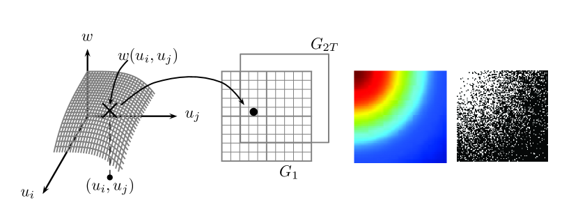
where G[i,j]𝐺𝑖𝑗G[i,j] denotes the (i,j)𝑖𝑗(i,j)th entry of the adjacency matrix representing a particular realization of 𝒢(n,w)𝒢𝑛𝑤\mathcal{G}(n,w) (See Figure 1). As an example, we note that the stochastic block-model is the case where w(x,y)𝑤𝑥𝑦w(x,y) is a piecewise constant function.

Refer to caption
Figure 1: [Left] Given a graphon w:[0,1]2[0,1]:𝑤superscript01201w:[0,1]^{2}\rightarrow[0,1], we draw i.i.d. samples uisubscript𝑢𝑖u_{i}, ujsubscript𝑢𝑗u_{j} from Uniform[0,1] and assign Gt[i,j]=1subscript𝐺𝑡𝑖𝑗1G_{t}[i,j]=1 with probability w(ui,uj)𝑤subscript𝑢𝑖subscript𝑢𝑗w(u_{i},u_{j}), for t=1,,2T𝑡12𝑇t=1,\ldots,2T. [Middle] Heat map of a graphon w𝑤w. [Right] A random graph generated by the graphon shown in the middle. Rows and columns of the graph are ordered by increasing uisubscript𝑢𝑖u_{i}, instead of i𝑖i for better visualization.

The problem of interest is defined as follows: Given a sequence of 2T2𝑇2T observed directed graphs G1,,G2Tsubscript𝐺1subscript𝐺2𝑇G_{1},\ldots,G_{2T}, can we make an estimate w^^𝑤\widehat{w} of w𝑤w, such that w^w^𝑤𝑤\widehat{w}\rightarrow w with high probability as n𝑛n goes to infinity? This question has been loosely attempted in the literature, but none of which has a complete solution. For example, Lloyd et al. (Lloyd et al. 2012) proposed a Bayesian estimator without a consistency proof; Choi and Wolfe (Choi and Wolfe ) studied the consistency properties, but did not provide algorithms to estimate the graphon. To the best of our knowledge, the only method that estimates graphons consistently, besides ours, is USVT (Chatterjee ). However, our algorithm has better complexity and outperforms USVT in our simulations. More recently, other groups have begun exploring approaches related to ours (Wolfe and Olhede 2013; P.Latouche and Robin 2013).

The proposed approximation procedure requires w𝑤w to be piecewise Lipschitz. The basic idea is to approximate w𝑤w by a two-dimensional step function w^^𝑤\widehat{w} with diminishing intervals as n𝑛n increases.The proposed method is called the Stochastic blockmodel approximation (SBA) algorithm, as the idea of using a two-dimensional step function for approximation is equivalent to using the stochastic block models (Choi et al. 2012; Nowicki and Snijders 2001a; Hoff 2008; Channarond et al. 2012; Rohe et al. 2011). The SBA algorithm is defined up to permutations of the nodes, so the estimated graphon is not canonical. However, this does not affect the consistency properties of the SBA algorithm, as the consistency is measured w.r.t. the graphon that generates the graphs.

2 Stochastic blockmodel approximation: Procedure

In this section we present the proposed SBA algorithm and discuss its basic properties.

2.1 Assumptions on graphons

We assume that w𝑤w is piecewise Lipschitz, i.e., there exists a sequence of non-overlaping intervals Ik=[αk1,αk]subscript𝐼𝑘subscript𝛼𝑘1subscript𝛼𝑘I_{k}=[\alpha_{k-1},\,\alpha_{k}] defined by 0=α0<<αK=10subscript𝛼0subscript𝛼𝐾10=\alpha_{0}<\ldots<\alpha_{K}=1, and a constant L>0𝐿0L>0 such that, for any (x1,y1)subscript𝑥1subscript𝑦1(x_{1},y_{1}) and (x2,y2)Iij=Ii×Ijsubscript𝑥2subscript𝑦2subscript𝐼𝑖𝑗subscript𝐼𝑖subscript𝐼𝑗(x_{2},y_{2})\in I_{ij}=I_{i}\times I_{j},

|w(x1,y1)w(x2,y2)|L(|x1x2|+|y1y2|).𝑤subscript𝑥1subscript𝑦1𝑤subscript𝑥2subscript𝑦2𝐿subscript𝑥1subscript𝑥2subscript𝑦1subscript𝑦2|w(x_{1},y_{1})-w(x_{2},y_{2})|\leq L\left(|x_{1}-x_{2}|+|y_{1}-y_{2}|\right).

For generality we assume w𝑤w to be asymmetric i.e., w(u,v)w(v,u)𝑤𝑢𝑣𝑤𝑣𝑢w(u,v)\not=w(v,u), so that symmetric graphons can be considered as a special case. Consequently, a random graph 𝒢(n,w)𝒢𝑛𝑤\mathcal{G}(n,w) generated by w𝑤w is directed, i.e., G[i,j]G[j,i]𝐺𝑖𝑗𝐺𝑗𝑖G[i,j]\not=G[j,i].

2.2 Similarity of graphon slices

The intuition of the proposed SBA algorithm is that if the graphon is smooth, neighboring cross-sections of the graphon should be similar. In other words, if two labels uisubscript𝑢𝑖u_{i} and ujsubscript𝑢𝑗u_{j} are close i.e., |uiuj|0subscript𝑢𝑖subscript𝑢𝑗0|u_{i}-u_{j}|\approx 0, then the difference between the row slices |w(ui,)w(uj,)|𝑤subscript𝑢𝑖𝑤subscript𝑢𝑗|w(u_{i},\cdot)-w(u_{j},\cdot)| and the column slices |w(,ui)w(,uj)|𝑤subscript𝑢𝑖𝑤subscript𝑢𝑗|w(\cdot,u_{i})-w(\cdot,u_{j})| should also be small. To measure the similarity between two labels using the graphon slices, we define the following distance

dij=12(01[w(x,ui)w(x,uj)]2𝑑x+01[w(ui,y)w(uj,y)]2𝑑y).subscript𝑑𝑖𝑗12superscriptsubscript01superscriptdelimited-[]𝑤𝑥subscript𝑢𝑖𝑤𝑥subscript𝑢𝑗2differential-d𝑥superscriptsubscript01superscriptdelimited-[]𝑤subscript𝑢𝑖𝑦𝑤subscript𝑢𝑗𝑦2differential-d𝑦d_{ij}=\frac{1}{2}\left(\int_{0}^{1}\left[w(x,u_{i})-w(x,u_{j})\right]^{2}dx+\int_{0}^{1}\left[w(u_{i},y)-w(u_{j},y)\right]^{2}dy\right). (2)

Thus, dijsubscript𝑑𝑖𝑗d_{ij} is small only if both row and column slices of the graphon are similar.

The usage of dijsubscript𝑑𝑖𝑗d_{ij} for graphon estimation will be discussed in the next subsection. But before we proceed, it should be noted that in practice dijsubscript𝑑𝑖𝑗d_{ij} has to be estimated from the observed graphs G1,,G2Tsubscript𝐺1subscript𝐺2𝑇G_{1},\ldots,G_{2T}. To derive an estimator d^ijsubscript^𝑑𝑖𝑗\widehat{d}_{ij} of dijsubscript𝑑𝑖𝑗d_{ij}, it is helpful to express dijsubscript𝑑𝑖𝑗d_{ij} in a way that the estimators can be easily obtained. To this end, we let

cij=01w(x,ui)w(x,uj)𝑑xandrij=01w(ui,y)w(uj,y)𝑑y,formulae-sequencesubscript𝑐𝑖𝑗superscriptsubscript01𝑤𝑥subscript𝑢𝑖𝑤𝑥subscript𝑢𝑗differential-d𝑥andsubscript𝑟𝑖𝑗superscriptsubscript01𝑤subscript𝑢𝑖𝑦𝑤subscript𝑢𝑗𝑦differential-d𝑦\displaystyle c_{ij}=\int_{0}^{1}w(x,u_{i})w(x,u_{j})dx\quad\quad\mbox{and}\quad\quad r_{ij}=\int_{0}^{1}w(u_{i},y)w(u_{j},y)dy,

and express dijsubscript𝑑𝑖𝑗d_{ij} as dij=12[(ciicijcji+cjj)+(riirijrji+rjj)]subscript𝑑𝑖𝑗12delimited-[]subscript𝑐𝑖𝑖subscript𝑐𝑖𝑗subscript𝑐𝑗𝑖subscript𝑐𝑗𝑗subscript𝑟𝑖𝑖subscript𝑟𝑖𝑗subscript𝑟𝑗𝑖subscript𝑟𝑗𝑗d_{ij}=\frac{1}{2}\Big{[}(c_{ii}-c_{ij}-c_{ji}+c_{jj})+(r_{ii}-r_{ij}-r_{ji}+r_{jj})\Big{]}. Inspecting this expression, we consider the following estimators for cijsubscript𝑐𝑖𝑗c_{ij} and rijsubscript𝑟𝑖𝑗r_{ij}:

c^ijksuperscriptsubscript^𝑐𝑖𝑗𝑘\displaystyle\widehat{c}_{ij}^{k} =1T2(1t1TGt1[k,i])(T<t22TGt2[k,j]),absent1superscript𝑇2subscript1subscript𝑡1𝑇subscript𝐺subscript𝑡1𝑘𝑖subscript𝑇subscript𝑡22𝑇subscript𝐺subscript𝑡2𝑘𝑗\displaystyle=\frac{1}{T^{2}}\left(\sum_{1\leq t_{1}\leq T}G_{t_{1}}[k,i]\right)\left(\sum_{T<t_{2}\leq 2T}G_{t_{2}}[k,j]\right), (3)
r^ijksuperscriptsubscript^𝑟𝑖𝑗𝑘\displaystyle\widehat{r}_{ij}^{k} =1T2(1t1TGt1[i,k])(T<t22TGt2[j,k]).absent1superscript𝑇2subscript1subscript𝑡1𝑇subscript𝐺subscript𝑡1𝑖𝑘subscript𝑇subscript𝑡22𝑇subscript𝐺subscript𝑡2𝑗𝑘\displaystyle=\frac{1}{T^{2}}\left(\sum_{1\leq t_{1}\leq T}G_{t_{1}}[i,k]\right)\left(\sum_{T<t_{2}\leq 2T}G_{t_{2}}[j,k]\right). (4)

Here, the superscript k𝑘k can be interpreted as the dummy variables x𝑥x and y𝑦y in defining cijsubscript𝑐𝑖𝑗c_{ij} and rijsubscript𝑟𝑖𝑗r_{ij}, respectively. Summing all possible k𝑘k’s yields an estimator d^ijsubscript^𝑑𝑖𝑗\widehat{d}_{ij} that looks similar to dijsubscript𝑑𝑖𝑗d_{ij}:

d^ij=12[1Sk𝒮{(r^iikr^ijkr^jik+r^jjk)+(c^iikc^ijkc^jik+c^jjk)}],subscript^𝑑𝑖𝑗12delimited-[]1𝑆subscript𝑘𝒮superscriptsubscript^𝑟𝑖𝑖𝑘superscriptsubscript^𝑟𝑖𝑗𝑘superscriptsubscript^𝑟𝑗𝑖𝑘superscriptsubscript^𝑟𝑗𝑗𝑘superscriptsubscript^𝑐𝑖𝑖𝑘superscriptsubscript^𝑐𝑖𝑗𝑘superscriptsubscript^𝑐𝑗𝑖𝑘superscriptsubscript^𝑐𝑗𝑗𝑘\widehat{d}_{ij}=\frac{1}{2}\left[\frac{1}{S}\sum_{k\in\mathcal{S}}\left\{\left(\widehat{r}_{ii}^{k}-\widehat{r}_{ij}^{k}-\widehat{r}_{ji}^{k}+\widehat{r}_{jj}^{k}\right)+\left(\widehat{c}_{ii}^{k}-\widehat{c}_{ij}^{k}-\widehat{c}_{ji}^{k}+\widehat{c}_{jj}^{k}\right)\right\}\right], (5)

where 𝒮={1,,n}\{i,j}𝒮\1𝑛𝑖𝑗\mathcal{S}=\{1,\ldots,n\}\backslash\{i,j\} is the set of summation indices.

The motivation of defining the estimators in (3) and (4) is that a row of the adjacency matrix G[i,]𝐺𝑖G[i,\cdot] is fully characterized by the corresponding row of the graphon w(ui,)𝑤subscript𝑢𝑖w(u_{i},\cdot). Thus the expected value of 1T(1t1TGt1[i,])1𝑇subscript1subscript𝑡1𝑇subscript𝐺subscript𝑡1𝑖\frac{1}{T}\left(\sum_{1\leq t_{1}\leq T}G_{t_{1}}[i,\cdot]\right) is w(ui,)𝑤subscript𝑢𝑖w(u_{i},\cdot), and hence 1Sk𝒮r^ijk1𝑆subscript𝑘𝒮superscriptsubscript^𝑟𝑖𝑗𝑘\frac{1}{S}\sum_{k\in\mathcal{S}}\widehat{r}_{ij}^{k} is an estimator for rijsubscript𝑟𝑖𝑗r_{ij}. To theoretically justify this intuition, we will show in Section 3 that d^ijsubscript^𝑑𝑖𝑗\widehat{d}_{ij} is indeed a good estimator: it is not only unbiased, but is also concentrated round dijsubscript𝑑𝑖𝑗d_{ij} for large n𝑛n. Furthermore, we will show that it is possible to use a random subset of 𝒮𝒮\mathcal{S} instead of {1,,n}\{i,j}\1𝑛𝑖𝑗\{1,\ldots,n\}\backslash\{i,j\} to achieve the same asymptotic behavior. As a result, the estimation of dijsubscript𝑑𝑖𝑗d_{ij} can be performed locally in a neighborhood of i𝑖i and j𝑗j, instead of all n𝑛n vertices.

2.3 Blocking the vertices

The similarity metric d^ijsubscript^𝑑𝑖𝑗\widehat{d}_{ij} discussed above suggests one simple method to approximate w𝑤w by a piecewise constant function w^^𝑤\widehat{w} (i.e., a stochastic block-model). Given G1,,G2Tsubscript𝐺1subscript𝐺2𝑇G_{1},\ldots,G_{2T}, we can cluster the (unknown) labels {u1,,un}subscript𝑢1subscript𝑢𝑛\{u_{1},\ldots,u_{n}\} into K𝐾K blocks B^1,,B^Ksubscript^𝐵1subscript^𝐵𝐾\widehat{B}_{1},\ldots,\widehat{B}_{K} using a procedure described below. Once the blocks B^1,,B^Ksubscript^𝐵1subscript^𝐵𝐾\widehat{B}_{1},\ldots,\widehat{B}_{K} are defined, we can then determine w^(ui,uj)^𝑤subscript𝑢𝑖subscript𝑢𝑗\widehat{w}(u_{i},u_{j}) by computing the empirical frequency of edges that are present across blocks B^isubscript^𝐵𝑖\widehat{B}_{i} and B^jsubscript^𝐵𝑗\widehat{B}_{j}:

w^(ui,uj)=1|B^i||B^j|ixB^ijyB^j12T(G1[ix,jy]+G2[ix,jy]++G2T[ix,jy]),^𝑤subscript𝑢𝑖subscript𝑢𝑗1subscript^𝐵𝑖subscript^𝐵𝑗subscriptsubscript𝑖𝑥subscript^𝐵𝑖subscriptsubscript𝑗𝑦subscript^𝐵𝑗12𝑇subscript𝐺1subscript𝑖𝑥subscript𝑗𝑦subscript𝐺2subscript𝑖𝑥subscript𝑗𝑦subscript𝐺2𝑇subscript𝑖𝑥subscript𝑗𝑦\widehat{w}(u_{i},u_{j})=\frac{1}{|\widehat{B}_{i}|\,|\widehat{B}_{j}|}\sum_{i_{x}\in\widehat{B}_{i}}\sum_{j_{y}\in\widehat{B}_{j}}\frac{1}{2T}\left(G_{1}[i_{x},j_{y}]+G_{2}[i_{x},j_{y}]+\ldots+G_{2T}[i_{x},j_{y}]\right), (6)

where B^isubscript^𝐵𝑖\widehat{B}_{i} is the block containing uisubscript𝑢𝑖u_{i} so that summing Gt[x,y]subscript𝐺𝑡𝑥𝑦G_{t}[x,y] over xB^i𝑥subscript^𝐵𝑖x\in\widehat{B}_{i} and yB^j𝑦subscript^𝐵𝑗y\in\widehat{B}_{j} yields an estimate of the expected number of edges linking block B^isubscript^𝐵𝑖\widehat{B}_{i} and B^jsubscript^𝐵𝑗\widehat{B}_{j}.

To cluster the unknown labels {u1,,un}subscript𝑢1subscript𝑢𝑛\{u_{1},\ldots,u_{n}\} we propose a greedy approach as shown in Algorithm 1. Starting with Ω={u1,,un}Ωsubscript𝑢1subscript𝑢𝑛\Omega=\{u_{1},\ldots,u_{n}\}, we randomly pick a node ipsubscript𝑖𝑝i_{p} and call it the pivot. Then for all other vertices ivΩ\{ip}subscript𝑖𝑣\Ωsubscript𝑖𝑝i_{v}\in\Omega\backslash\{i_{p}\}, we compute the distance d^ip,ivsubscript^𝑑subscript𝑖𝑝subscript𝑖𝑣\widehat{d}_{i_{p},i_{v}} and check whether d^ip,iv<Δ2subscript^𝑑subscript𝑖𝑝subscript𝑖𝑣superscriptΔ2\widehat{d}_{i_{p},i_{v}}<\Delta^{2} for some precision parameter Δ>0Δ0\Delta>0. If d^ip,iv<Δ2subscript^𝑑subscript𝑖𝑝subscript𝑖𝑣superscriptΔ2\widehat{d}_{i_{p},i_{v}}<\Delta^{2}, then we assign ivsubscript𝑖𝑣i_{v} to the same block as ipsubscript𝑖𝑝i_{p}. Therefore, after scanning through ΩΩ\Omega once, a block B^1={ip,iv1,iv2,}subscript^𝐵1subscript𝑖𝑝subscript𝑖subscript𝑣1subscript𝑖subscript𝑣2\widehat{B}_{1}=\{i_{p},i_{v_{1}},i_{v_{2}},\ldots\} will be defined. By updating ΩΩ\Omega as ΩΩ\B^1Ω\Ωsubscript^𝐵1\Omega\leftarrow\Omega\backslash\widehat{B}_{1}, the process repeats until Ω=Ω\Omega=\emptyset.

The proposed greedy algorithm is only a local solution in a sense that it does not return the globally optimal clusters. However, as will be shown in Section 3, although the clustering algorithm is not globally optimal, the estimated graphon w^^𝑤\widehat{w} is still guaranteed to be a consistent estimate of the true graphon w𝑤w as n𝑛n\rightarrow\infty. Since the greedy algorithm is numerically efficient, it serves as a practical computational tool to estimate w𝑤w.

2.4 Main algorithm

Algorithm 1 Stochastic blockmodel approximation
  Input: A set of observed graphs G1,,G2Tsubscript𝐺1subscript𝐺2𝑇G_{1},\ldots,G_{2T} and the precision parameter ΔΔ\Delta.
  Output: Estimated stochastic blocks B^1,,B^Ksubscript^𝐵1subscript^𝐵𝐾\widehat{B}_{1},\ldots,\widehat{B}_{K}.
  Initialize: Ω={1,,n}Ω1𝑛\Omega=\{1,\ldots,n\}, and k=1𝑘1k=1.
  while ΩΩ\Omega\not=\emptyset do
     Randomly choose a vertex ipsubscript𝑖𝑝i_{p} from ΩΩ\Omega and assign it as the pivot for B^ksubscript^𝐵𝑘\widehat{B}_{k}: B^kipsubscript^𝐵𝑘subscript𝑖𝑝\widehat{B}_{k}\leftarrow i_{p}.
     for Every other vertices ivΩ\{ip}subscript𝑖𝑣\Ωsubscript𝑖𝑝i_{v}\in\Omega\backslash\{i_{p}\} do
        Compute the distance estimate d^ip,ivsubscript^𝑑subscript𝑖𝑝subscript𝑖𝑣\widehat{d}_{i_{p},i_{v}}.
        If d^ip,ivΔ2subscript^𝑑subscript𝑖𝑝subscript𝑖𝑣superscriptΔ2\widehat{d}_{i_{p},i_{v}}\leq\Delta^{2}, then assign ivsubscript𝑖𝑣i_{v} as a member of B^ksubscript^𝐵𝑘\widehat{B}_{k}: B^kivsubscript^𝐵𝑘subscript𝑖𝑣\widehat{B}_{k}\leftarrow i_{v}.
     end for
     Update ΩΩ\Omega: ΩΩ\B^kΩ\Ωsubscript^𝐵𝑘\Omega\leftarrow\Omega\backslash\widehat{B}_{k}.
     Update counter: kk+1𝑘𝑘1k\leftarrow k+1.
  end while

Algorithm 1 illustrates the pseudo-code for the proposed stochastic block-model approximation. The complexity of this algorithm is 𝒪(TSKn)𝒪𝑇𝑆𝐾𝑛\mathcal{O}(TSKn), where T𝑇T is half the number of observations, S𝑆S is the size of the neighborhood, K𝐾K is the number of blocks and n𝑛n is number of vertices of the graph.

3 Stochastic blockmodel approximation: Theory of estimation

In this section we present the theoretical aspects of the proposed SBA algorithm. We will first discuss the properties of the estimator d^ijsubscript^𝑑𝑖𝑗\widehat{d}_{ij}, and then show the consistency of the estimated graphon w^^𝑤\widehat{w}. Details of the proofs can be found in the supplementary material.

3.1 Concentration analysis of d^ijsubscript^𝑑𝑖𝑗\widehat{d}_{ij}

Our first theorem below shows that the proposed estimator d^ijsubscript^𝑑𝑖𝑗\widehat{d}_{ij} is both unbiased, and is concentrated around its expected value dijsubscript𝑑𝑖𝑗d_{ij}.

Theorem 1.

The estimator d^ijsubscript^𝑑𝑖𝑗\widehat{d}_{ij} for dijsubscript𝑑𝑖𝑗d_{ij} is unbiased, i.e., 𝔼[d^ij]=dij𝔼delimited-[]subscript^𝑑𝑖𝑗subscript𝑑𝑖𝑗\mathbb{E}[\widehat{d}_{ij}]=d_{ij}. Further, for any ϵ>0italic-ϵ0\epsilon>0,

Pr[|d^ijdij|>ϵ]8eSϵ232/T+8ϵ/3,Prsubscript^𝑑𝑖𝑗subscript𝑑𝑖𝑗italic-ϵ8superscript𝑒𝑆superscriptitalic-ϵ232𝑇8italic-ϵ3\Pr\left[\left|\widehat{d}_{ij}-d_{ij}\right|>\epsilon\right]\leq 8e^{-\frac{S\epsilon^{2}}{32/T+8\epsilon/3}}, (7)

where S𝑆S is the size of the neighborhood 𝒮𝒮\mathcal{S}, and 2T2𝑇2T is the number of observations.

Proof.

Here we only highlight the important steps to present the intuition. The basic idea of the proof is to zoom-in a microscopic term of r^ijksuperscriptsubscript^𝑟𝑖𝑗𝑘\widehat{r}_{ij}^{k} and show that it is unbiased. To this end, we use the fact that Gt1[i,k]subscript𝐺subscript𝑡1𝑖𝑘G_{t_{1}}[i,k] and Gt2[j,k]subscript𝐺subscript𝑡2𝑗𝑘G_{t_{2}}[j,k] are conditionally independent on uksubscript𝑢𝑘u_{k} to show

𝔼[Gt1[i,k]Gt2[j,k]|uk]𝔼delimited-[]conditionalsubscript𝐺subscript𝑡1𝑖𝑘subscript𝐺subscript𝑡2𝑗𝑘subscript𝑢𝑘\displaystyle\mathbb{E}[G_{t_{1}}[i,k]G_{t_{2}}[j,k]\;|\;u_{k}] =Pr[Gt1[i,k]=1,Gt2[j,k]=1|uk]absentPrsubscript𝐺subscript𝑡1𝑖𝑘1subscript𝐺subscript𝑡2𝑗𝑘conditional1subscript𝑢𝑘\displaystyle=\Pr[G_{t_{1}}[i,k]=1,G_{t_{2}}[j,k]=1\;|\;u_{k}]
=(a)Pr[Gt1[i,k]=1|uk]Pr[Gt2[j,k]=1|uk]𝑎Prsubscript𝐺subscript𝑡1𝑖𝑘conditional1subscript𝑢𝑘Prsubscript𝐺subscript𝑡2𝑗𝑘conditional1subscript𝑢𝑘\displaystyle\overset{(a)}{=}\Pr[G_{t_{1}}[i,k]=1\;|\;u_{k}]\Pr[G_{t_{2}}[j,k]=1\;|\;u_{k}]
=w(ui,uk)w(uj,uk),absent𝑤subscript𝑢𝑖subscript𝑢𝑘𝑤subscript𝑢𝑗subscript𝑢𝑘\displaystyle=w(u_{i},u_{k})w(u_{j},u_{k}),

which then implies 𝔼[r^ijk|uk]=w(ui,uk)w(uj,uk)𝔼delimited-[]conditionalsuperscriptsubscript^𝑟𝑖𝑗𝑘subscript𝑢𝑘𝑤subscript𝑢𝑖subscript𝑢𝑘𝑤subscript𝑢𝑗subscript𝑢𝑘\mathbb{E}[\widehat{r}_{ij}^{k}\;|\;u_{k}]=w(u_{i},u_{k})w(u_{j},u_{k}), and by iterated expectation we have 𝔼[r^ijk]=𝔼[𝔼[r^ijk|uk]]=rij𝔼delimited-[]superscriptsubscript^𝑟𝑖𝑗𝑘𝔼delimited-[]𝔼delimited-[]conditionalsuperscriptsubscript^𝑟𝑖𝑗𝑘subscript𝑢𝑘subscript𝑟𝑖𝑗\mathbb{E}[\widehat{r}_{ij}^{k}]=\mathbb{E}[\mathbb{E}[\widehat{r}_{ij}^{k}\;|\;u_{k}]]=r_{ij}. The concentration inequality follows from a similar idea to bound the variance of r^ijksuperscriptsubscript^𝑟𝑖𝑗𝑘\widehat{r}_{ij}^{k} and apply Bernstein’s inequality. ∎

That Gt1[i,k]subscript𝐺subscript𝑡1𝑖𝑘G_{t_{1}}[i,k] and Gt2[j,k]subscript𝐺subscript𝑡2𝑗𝑘G_{t_{2}}[j,k] are conditionally independent on uksubscript𝑢𝑘u_{k} is a critical fact for the success of the proposed algorithm. It also explains why at least 2 independently observed graphs are necessary, for otherwise we cannot separate the probability in the second equality above marked with (a)𝑎(a).

3.2 Choosing the number of blocks

The performance of the Algorithm 1 is sensitive to the number of blocks it defines. On the one hand, it is desirable to have more blocks so that the graphon can be finely approximated. But on the other hand, if the number of blocks is too large then each block will contain only few vertices. This is bad because in order to estimate the value on each block, a sufficient number of vertices in each block is required. The trade-off between these two cases is controlled by the precision parameter ΔΔ\Delta: a large ΔΔ\Delta generates few large clusters, while small ΔΔ\Delta generates many small clusters. A precise relationship between the ΔΔ\Delta and K𝐾K, the number of blocks generated the algorithm, is given in Theorem 2.

Theorem 2.

Let ΔΔ\Delta be the accuracy parameter and K𝐾K be the number of blocks estimated by Algorithm 1, then

Pr[K>QL2Δ]8n2eSΔ4128/T+16Δ2/3,Pr𝐾𝑄𝐿2Δ8superscript𝑛2superscript𝑒𝑆superscriptΔ4128𝑇16superscriptΔ23\Pr\left[K>\frac{QL\sqrt{2}}{\Delta}\right]\leq 8n^{2}e^{-\frac{S\Delta^{4}}{128/T+16\Delta^{2}/3}}, (8)

where L𝐿L is the Lipschitz constant and Q𝑄Q is the number of Lipschitz blocks in w𝑤w.

In practice, we estimate ΔΔ\Delta using a cross-validation scheme to find the optimal 2D histogram bin width (Wasserman 2005). The idea is to test a sequence of potential values of ΔΔ\Delta and seek the one that minimizes the cross validation risk, defined as

J^(Δ)=2h(n1)n+1h(n1)j=1Kp^j2,^𝐽Δ2𝑛1𝑛1𝑛1superscriptsubscript𝑗1𝐾superscriptsubscript^𝑝𝑗2\widehat{J}(\Delta)=\frac{2}{h(n-1)}-\frac{n+1}{h(n-1)}\sum_{j=1}^{K}\widehat{p}_{j}^{2}, (9)

where p^j=|B^j|/nsubscript^𝑝𝑗subscript^𝐵𝑗𝑛\widehat{p}_{j}=|\widehat{B}_{j}|/n and h=1/K1𝐾h=1/K. Algorithm 2 details the proposed cross-validation scheme.

Algorithm 2 Cross Validation
  Input: Graphs G1,,G2Tsubscript𝐺1subscript𝐺2𝑇G_{1},\ldots,G_{2T}.
  Output: Blocks B^1,,B^Ksubscript^𝐵1subscript^𝐵𝐾\widehat{B}_{1},\ldots,\widehat{B}_{K}, and optimal ΔΔ\Delta.
  for a sequence of ΔΔ\Delta’s do
     Estimate blocks B^1,,B^Ksubscript^𝐵1subscript^𝐵𝐾\widehat{B}_{1},\ldots,\widehat{B}_{K} from G1,,G2Tsubscript𝐺1subscript𝐺2𝑇G_{1},\ldots,G_{2T}. [Algorithm 1]
     Compute p^j=|B^j|/nsubscript^𝑝𝑗subscript^𝐵𝑗𝑛\widehat{p}_{j}=|\widehat{B}_{j}|/n, for j=1,,K𝑗1𝐾j=1,\ldots,K.
     Compute J^(Δ)=2h(n1)n+1h(n1)j=1Kp^j2^𝐽Δ2𝑛1𝑛1𝑛1superscriptsubscript𝑗1𝐾superscriptsubscript^𝑝𝑗2\widehat{J}(\Delta)=\frac{2}{h(n-1)}-\frac{n+1}{h(n-1)}\sum_{j=1}^{K}\widehat{p}_{j}^{2}, with h=1/K1𝐾h=1/K.
  end for
  Pick the ΔΔ\Delta with minimum J^(Δ)^𝐽Δ\widehat{J}(\Delta), and the corresponding B^1,,B^Ksubscript^𝐵1subscript^𝐵𝐾\widehat{B}_{1},\ldots,\widehat{B}_{K}.

3.3 Consistency of w^^𝑤\widehat{w}

The goal of our next theorem is to show that w^^𝑤\widehat{w} is a consistent estimate of w𝑤w, i.e., w^w^𝑤𝑤\widehat{w}\rightarrow w as n𝑛n\rightarrow\infty. To begin with, let us first recall two commonly used metric:

Definition 1.

The mean squared error (MSE) and mean absolute error (MAE) are defined as

MSE(w^)MSE^𝑤\displaystyle\mathrm{MSE}(\widehat{w}) =1n2iv=1njv=1n(w(uiv,ujv)w^(uiv,ujv))2absent1superscript𝑛2superscriptsubscriptsubscript𝑖𝑣1𝑛superscriptsubscriptsubscript𝑗𝑣1𝑛superscript𝑤subscript𝑢subscript𝑖𝑣subscript𝑢subscript𝑗𝑣^𝑤subscript𝑢subscript𝑖𝑣subscript𝑢subscript𝑗𝑣2\displaystyle=\frac{1}{n^{2}}\sum_{i_{v}=1}^{n}\sum_{j_{v}=1}^{n}\left(w(u_{i_{v}},u_{j_{v}})-\widehat{w}(u_{i_{v}},u_{j_{v}})\right)^{2}
MAE(w^)MAE^𝑤\displaystyle\mathrm{MAE}(\widehat{w}) =1n2iv=1njv=1n|w(uiv,ujv)w^(uiv,ujv)|.absent1superscript𝑛2superscriptsubscriptsubscript𝑖𝑣1𝑛superscriptsubscriptsubscript𝑗𝑣1𝑛𝑤subscript𝑢subscript𝑖𝑣subscript𝑢subscript𝑗𝑣^𝑤subscript𝑢subscript𝑖𝑣subscript𝑢subscript𝑗𝑣\displaystyle=\frac{1}{n^{2}}\sum_{i_{v}=1}^{n}\sum_{j_{v}=1}^{n}\left|w(u_{i_{v}},u_{j_{v}})-\widehat{w}(u_{i_{v}},u_{j_{v}})\right|.
Theorem 3.

If SΘ(n)𝑆Θ𝑛S\in\Theta(n) and Δω((log(n)n)14)o(1)Δ𝜔superscript𝑛𝑛14𝑜1\Delta\in\omega\left(\left(\frac{\log(n)}{n}\right)^{\frac{1}{4}}\right)\cap o(1), then

limn𝔼[MAE(w^)]=0andlimn𝔼[MSE(w^)]=0.formulae-sequencesubscript𝑛𝔼delimited-[]MAE^𝑤0andsubscript𝑛𝔼delimited-[]MSE^𝑤0\lim_{n\rightarrow\infty}\mathbb{E}[\mathrm{MAE}(\widehat{w})]=0\quad\quad\mbox{and}\quad\quad\lim_{n\rightarrow\infty}\mathbb{E}[\mathrm{MSE}(\widehat{w})]=0.
Proof.

The details of the proof can be found in the supplementary material . Here we only outline the key steps to present the intuition of the theorem. The goal of Theorem 29 is to show convergence of |w^(ui,uj)w(ui,uj)|^𝑤subscript𝑢𝑖subscript𝑢𝑗𝑤subscript𝑢𝑖subscript𝑢𝑗|\widehat{w}(u_{i},u_{j})-w(u_{i},u_{j})|. The idea is to consider the following two quantities:

w¯(ui,uj)¯𝑤subscript𝑢𝑖subscript𝑢𝑗\displaystyle\overline{w}(u_{i},u_{j}) =1|B^i||B^j|ixB^ijxB^jw(uix,ujx),absent1subscript^𝐵𝑖subscript^𝐵𝑗subscriptsubscript𝑖𝑥subscript^𝐵𝑖subscriptsubscript𝑗𝑥subscript^𝐵𝑗𝑤subscript𝑢subscript𝑖𝑥subscript𝑢subscript𝑗𝑥\displaystyle=\frac{1}{|\widehat{B}_{i}|\,|\widehat{B}_{j}|}\sum_{i_{x}\in\widehat{B}_{i}}\sum_{j_{x}\in\widehat{B}_{j}}w(u_{i_{x}},u_{j_{x}}),
w^(ui,uj)^𝑤subscript𝑢𝑖subscript𝑢𝑗\displaystyle\widehat{w}(u_{i},u_{j}) =1|B^i||B^j|ixB^ijyB^j12T(G1[ix,jy]+G2[ix,jy]++G2T[ix,jy]),absent1subscript^𝐵𝑖subscript^𝐵𝑗subscriptsubscript𝑖𝑥subscript^𝐵𝑖subscriptsubscript𝑗𝑦subscript^𝐵𝑗12𝑇subscript𝐺1subscript𝑖𝑥subscript𝑗𝑦subscript𝐺2subscript𝑖𝑥subscript𝑗𝑦subscript𝐺2𝑇subscript𝑖𝑥subscript𝑗𝑦\displaystyle=\frac{1}{|\widehat{B}_{i}|\,|\widehat{B}_{j}|}\sum_{i_{x}\in\widehat{B}_{i}}\sum_{j_{y}\in\widehat{B}_{j}}\frac{1}{2T}\left(G_{1}[i_{x},j_{y}]+G_{2}[i_{x},j_{y}]+\ldots+G_{2T}[i_{x},j_{y}]\right),

so that if we can bound |w¯(ui,uj)w(ui,uj)|¯𝑤subscript𝑢𝑖subscript𝑢𝑗𝑤subscript𝑢𝑖subscript𝑢𝑗|\overline{w}(u_{i},u_{j})-w(u_{i},u_{j})| and |w¯(ui,uj)w^(ui,uj)|¯𝑤subscript𝑢𝑖subscript𝑢𝑗^𝑤subscript𝑢𝑖subscript𝑢𝑗|\overline{w}(u_{i},u_{j})-\widehat{w}(u_{i},u_{j})|, then consequently |w^(ui,uj)w(ui,uj)|^𝑤subscript𝑢𝑖subscript𝑢𝑗𝑤subscript𝑢𝑖subscript𝑢𝑗|\widehat{w}(u_{i},u_{j})-w(u_{i},u_{j})| can also be bounded.

The bound for the first term |w¯(ui,uj)w(ui,uj)|¯𝑤subscript𝑢𝑖subscript𝑢𝑗𝑤subscript𝑢𝑖subscript𝑢𝑗|\overline{w}(u_{i},u_{j})-w(u_{i},u_{j})| is shown in Lemma 1: By Algorithm 1, any vertex ivB^isubscript𝑖𝑣subscript^𝐵𝑖i_{v}\in\widehat{B}_{i} is guaranteed to be within a distance ΔΔ\Delta from the pivot of B^isubscript^𝐵𝑖\widehat{B}_{i}. Since w¯(ui,uj)¯𝑤subscript𝑢𝑖subscript𝑢𝑗\overline{w}(u_{i},u_{j}) is an average over B^isubscript^𝐵𝑖\widehat{B}_{i} and B^jsubscript^𝐵𝑗\widehat{B}_{j}, by Theorem 1 a probability bound involving ΔΔ\Delta can be obtained.

The bound for the second term |w¯(ui,uj)w^(ui,uj)|¯𝑤subscript𝑢𝑖subscript𝑢𝑗^𝑤subscript𝑢𝑖subscript𝑢𝑗|\overline{w}(u_{i},u_{j})-\widehat{w}(u_{i},u_{j})| is shown in Lemma 2. Different from Lemma 1, here we need to consider two possible situations: either the intermediate estimate w¯(ui,uj)¯𝑤subscript𝑢𝑖subscript𝑢𝑗\overline{w}(u_{i},u_{j}) is close to the ground truth w(ui,uj)𝑤subscript𝑢𝑖subscript𝑢𝑗w(u_{i},u_{j}), or w¯(ui,uj)¯𝑤subscript𝑢𝑖subscript𝑢𝑗\overline{w}(u_{i},u_{j}) is far from the ground truth w(ui,uj)𝑤subscript𝑢𝑖subscript𝑢𝑗w(u_{i},u_{j}). This accounts for the sum in Lemma 2. Individual bounds are derived based on Lemma 1 and Theorem 1.

Combining Lemma 1 and Lemma 2, we can then bound the error and show convergence. ∎

Lemma 1.

For any ivB^isubscript𝑖𝑣subscript^𝐵𝑖i_{v}\in\widehat{B}_{i} and jvB^jsubscript𝑗𝑣subscript^𝐵𝑗j_{v}\in\widehat{B}_{j},

Pr[|w¯(ui,uj)w(uiv,ujv)|>8Δ1/2L1/4]32|B^i||B^j|eSΔ432/T+8Δ2/3.Pr¯𝑤subscript𝑢𝑖subscript𝑢𝑗𝑤subscript𝑢subscript𝑖𝑣subscript𝑢subscript𝑗𝑣8superscriptΔ12superscript𝐿1432subscript^𝐵𝑖subscript^𝐵𝑗superscript𝑒𝑆superscriptΔ432𝑇8superscriptΔ23\Pr\left[|\overline{w}(u_{i},u_{j})-w(u_{i_{v}},u_{j_{v}})|>8\Delta^{1/2}L^{1/4}\right]\leq 32|\widehat{B}_{i}|\,|\widehat{B}_{j}|e^{-\frac{S\Delta^{4}}{32/T+8\Delta^{2}/3}}. (10)
Lemma 2.

For any ivB^isubscript𝑖𝑣subscript^𝐵𝑖i_{v}\in\widehat{B}_{i} and jvB^jsubscript𝑗𝑣subscript^𝐵𝑗j_{v}\in\widehat{B}_{j},

Pr[|w^ijw¯ij|>8Δ1/2L1/4]2e256(T|B^i||B^j|LΔ)+32|B^i|2|B^j|2eSΔ432/T+8Δ2/3).\Pr\left[|\widehat{w}_{ij}-\overline{w}_{ij}|>8\Delta^{1/2}L^{1/4}\right]\leq 2e^{-256(T|\widehat{B}_{i}|\,|\widehat{B}_{j}|\sqrt{L}\Delta)}+32|\widehat{B}_{i}|^{2}|\widehat{B}_{j}|^{2}e^{-\frac{S\Delta^{4}}{32/T+8\Delta^{2}/3)}}. (11)

The condition SΘ(n)𝑆Θ𝑛S\in\Theta(n) is necessary to make Theorem 29 valid, because if S𝑆S is independent of n𝑛n, it is not possible to drive (10) and (11) to 00 even if n𝑛n\rightarrow\infty. The other condition on ΔΔ\Delta is also important as it forces the numerators and denominators in the exponentials of (10) and (11) to be well behaved.

4 Experiments

In this section we evaluate the proposed SBA algorithm by showing some empirical results. For the purpose of comparison, we consider (i) the universal singular value thresholding (USVT) (Chatterjee ); (ii) the largest-gap algorithm (LG) (Channarond et al. 2012); (iii) matrix completion from few entries (OptSpace) (Keshavan et al. 2010).

4.1 Estimating stochastic blockmodels

Accuracy as a function of growing graph size.

Our first experiment is to evaluate the proposed SBA algorithm for estimating stochastic blockmodels. For this purpose, we generate (arbitrarily) a graphon

w=[0.80.90.40.50.10.60.30.20.30.20.80.30.40.10.20.9],𝑤matrix0.80.90.40.50.10.60.30.20.30.20.80.30.40.10.20.9w=\begin{bmatrix}0.8&0.9&0.4&0.5\\ 0.1&0.6&0.3&0.2\\ 0.3&0.2&0.8&0.3\\ 0.4&0.1&0.2&0.9\end{bmatrix}, (12)

which represents a piecewise constant function with 4×4444\times 4 equi-space blocks.

Refer to caption Refer to caption
(a) Growing graph size, n𝑛n (b) Growing no. observations, 2T2𝑇2T
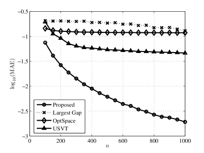
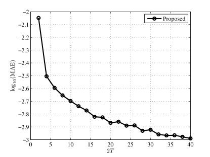
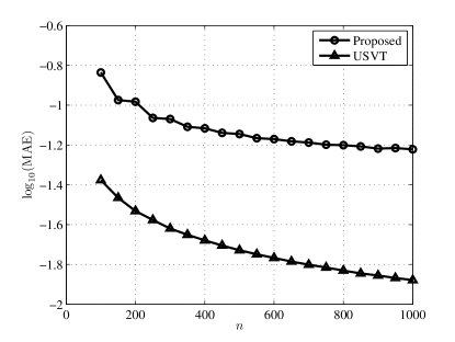
Figure 2: (a) MAE reduces as graph size grows. For the fairness of the amount of data that can be used, we use n2×n2×2𝑛2𝑛22\frac{n}{2}\times\frac{n}{2}\times 2 observations for SBA, and n×n×1𝑛𝑛1n\times n\times 1 observation for USVT (Chatterjee ) and LG (Channarond et al. 2012). (b) MAE of the proposed SBA algorithm reduces when more observations T𝑇T is available. Both plots are averaged over 100 independent trials.

Since USVT and LG use only one observed graph whereas the proposed SBA require at least 222 observations, in order to make the comparison fair, we use half of the nodes for SBA by generating two independent n2×n2𝑛2𝑛2\frac{n}{2}\times\frac{n}{2} observed graphs. For USVT and LG, we use one n×n𝑛𝑛n\times n observed graph.

Figure 2(a) shows the asymptotic behavior of the algorithms when n𝑛n grows. Figure 2(b) shows the estimation error of SBA algorithm as T𝑇T grows for graphs of size 200 vertices.

Accuracy as a function of growing number of blocks.

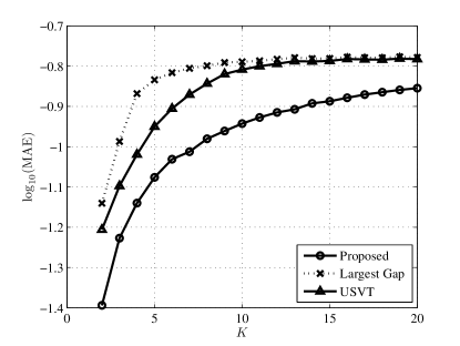
Our second experiment is to evaluate the performance of the algorithms as K𝐾K, the number of blocks, increases. To this end, we consider a sequence of K𝐾K, and for each K𝐾K we generate a graphon w𝑤w of K×K𝐾𝐾K\times K blocks. Each entry of the block is a random number generated from Uniform[0,1]Uniform01\mbox{Uniform}[0,1]. Same as the previous experiment, we fix n=200𝑛200n=200 and T=1𝑇1T=1. The experiment is repeated over 100 trials so that in every trial a different graphon is generated. The result shown in Figure 3(a) indicates that while estimation error increases as K𝐾K grows, the proposed SBA algorithm still attains the lowest MAE for all K𝐾K.

Refer to caption Refer to caption
(a) Growing no. blocks, K𝐾K (b) Missing links
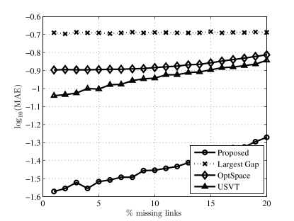
Figure 3: (a) As K𝐾K increases, MAE of all three algorithm increases but SBA still attains the lowest MAE. Here, we use n2×n2×2𝑛2𝑛22\frac{n}{2}\times\frac{n}{2}\times 2 observations for SBA, and n×n×1𝑛𝑛1n\times n\times 1 observation for USVT (Chatterjee ) and LG (Channarond et al. 2012). (b) Estimation of graphon in the presence of missing links: As the amount of missing links increases, estimation error also increases.

4.2 Estimation with missing edges

Our next experiment is to evaluate the performance of proposed SBA algorithm when there are missing edges in the observed graph. To model missing edges, we construct an n×n𝑛𝑛n\times n binary matrix M𝑀M with probability Pr[M[i,j]=0]=ξPr𝑀𝑖𝑗0𝜉\Pr[M[i,j]=0]=\xi, where 0ξ10𝜉10\leq\xi\leq 1 defines the percentage of missing edges. Given ξ𝜉\xi, 2T2𝑇2T matrices are generated with missing edges, and the observed graphs are defined as M1G1,,M2TG2Tdirect-productsubscript𝑀1subscript𝐺1direct-productsubscript𝑀2𝑇subscript𝐺2𝑇M_{1}\odot G_{1},\ldots,M_{2T}\odot G_{2T}, where direct-product\odot denotes the element-wise multiplication. The goal is to study how well SBA can reconstruct the graphon w^^𝑤\widehat{w} in the presence of missing links.

The modification of the proposed SBA algorithm for the case missing links is minimal: when computing (6), instead of averaging over all ixB^isubscript𝑖𝑥subscript^𝐵𝑖i_{x}\in\widehat{B}_{i} and jyB^jsubscript𝑗𝑦subscript^𝐵𝑗j_{y}\in\widehat{B}_{j}, we only average ixB^isubscript𝑖𝑥subscript^𝐵𝑖i_{x}\in\widehat{B}_{i} and jyB^jsubscript𝑗𝑦subscript^𝐵𝑗j_{y}\in\widehat{B}_{j} that are not masked out by all Msuperscript𝑀M^{\prime}s. Figure 3(b) shows the result of average over 100 independent trials. Here, we consider the graphon given in (12), with n=200𝑛200n=200 and T=1𝑇1T=1. It is evident that SBA outperforms its counterparts at a lower rate of missing links.

4.3 Estimating continuous graphons

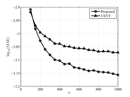
Our final experiment is to evaluate the proposed SBA algorithm in estimating continuous graphons. Here, we consider two of the graphons reported in (Chatterjee ):

w1(u,v)=11+exp{50(u2+v2)},andw2(u,v)=uv,formulae-sequencesubscript𝑤1𝑢𝑣1150superscript𝑢2superscript𝑣2andsubscript𝑤2𝑢𝑣𝑢𝑣\displaystyle w_{1}(u,v)=\frac{1}{1+\exp\{-50(u^{2}+v^{2})\}},\quad\mbox{and}\quad w_{2}(u,v)=uv,

where u,v[0,1]𝑢𝑣01u,v\in[0,1]. Here, w2subscript𝑤2w_{2} can be considered as a special case of the Eigenmodel (Hoff 2008) or latent feature relational model (Miller et al. 2009).

The results in Figure 4 shows that while both algorithms have improved estimates when n𝑛n grows, the performance depends on which of w1subscript𝑤1w_{1} and w2subscript𝑤2w_{2} that we are studying. This suggests that in practice the choice of the algorithm should depend on the expected structure of the graphon to be estimated: If the graph generated by the graphon demonstrates some low-rank properties, then USVT is likely to be a better option. For more structured or complex graphons the proposed procedure is recommended.
Refer to caption Refer to caption
(a) graphon w1subscript𝑤1w_{1} (b) graphon w2subscript𝑤2w_{2}
Figure 4: Comparison between SBA and USVT in estimating two continuous graphons w1subscript𝑤1w_{1} and w2subscript𝑤2w_{2}. Evidently, SBA performs better for w1subscript𝑤1w_{1} (high-rank) and worse for w2subscript𝑤2w_{2} (low-rank).

5 Concluding remarks

We presented a new computational tool for estimating graphons. The proposed algorithm approximates the continuous graphon by a stochastic block-model, in which the first step is to cluster the unknown vertex labels into blocks by using an empirical estimate of the distance between two graphon slices, and the second step is to build an empirical histogram to estimate the graphon. Complete consistency analysis of the algorithm is derived. The algorithm was evaluated experimentally, and we found that the algorithm is effective in estimating block structured graphons.

Code. An implementation of the stochastic blockmodel approximation (SBA) algorithm proposed in this paper is available online at: https://github.com/airoldilab/SBA

Acknowledgments. EMA is partially supported by NSF CAREER award IIS-1149662, ARO MURI award W911NF-11-1-0036, and an Alfred P. Sloan Research Fellowship. SHC is partially supported by a Croucher Foundation Post-Doctoral Research Fellowship.

References

  • Airoldi et al. (2008) E.M. Airoldi, D.M. Blei, S.E. Fienberg, and E.P. Xing. Mixed-membership stochastic blockmodels. Journal of Machine Learning Research, 9:1981–2014, 2008.
  • Aldous (1981) D.J. Aldous. Representations for partially exchangeable arrays of random variables. Journal of Multivariate Analysis, 11:581–598, 1981.
  • Azari and Airoldi (2012) H. Azari and E. M. Airoldi. Graphlet decomposition of a weighted network. Journal of Machine Learning Research, W&CP, 22:54–63, 2012.
  • Bickel and Chen (2009) P.J. Bickel and A. Chen. A nonparametric view of network models and Newman-Girvan and other modularities. Proc. Natl. Acad. Sci. USA, 106:21068–21073, 2009.
  • Bickel et al. (2011) P.J. Bickel, A. Chen, and E. Levina. The method of moments and degree distributions for network models. Annals of Statistics, 39(5):2280–2301, 2011.
  • Borgs et al. (2006) C. Borgs, J. Chayes, L. Lovász, V. T. Sós, B. Szegedy, and K. Vesztergombi. Graph limits and parameter testing. In Proc. ACM Symposium on Theory of Computing, pages 261–270, 2006.
  • Channarond et al. (2012) A. Channarond, J. Daudin, and S. Robin. Classification and estimation in the Stochastic Blockmodel based on the empirical degrees. Electronic Journal of Statistics, 6:2574–2601, 2012.
  • (8) S. Chatterjee. Matrix estimation by universal singular value thresholding. ArXiv:1212.1247. 2012.
  • (9) D.S. Choi and P.J. Wolfe. Co-clustering separately exchangeable network data. ArXiv:1212.4093. 2012.
  • Choi et al. (2012) D.S. Choi, P.J. Wolfe, and E.M. Airoldi. Stochastic blockmodels with a growing number of classes. Biometrika, 99:273–284, 2012.
  • Diaconis and Janson (2008) P. Diaconis and S. Janson. Graph limits and exchangeable random graphs. Rendiconti di Matematica e delle sue Applicazioni, Series VII, pages 33–61, 2008.
  • Fienberg et al. (1985) S. E. Fienberg, M. M. Meyer, and S. Wasserman. Statistical analysis of multiple sociometric relations. Journal of the American Statistical Association, 80:51–67, 1985.
  • Goldenberg et al. (2009) A. Goldenberg, A.X. Zheng, S.E. Fienberg, and E.M. Airoldi. A survey of statistical network models. Foundations and Trends in Machine Learning, 2:129–233, 2009.
  • Handcock et al. (2007) M. Handcock, A. E. Raftery, and J. Tantrum. Model-based clustering for social networks (with discussion). Journal of the Royal Statistical Society, Series A, 170:301–354, 2007.
  • Hoff (2008) P.D. Hoff. Modeling homophily and stochastic equivalence in symmetric relational data. In Neural Information Processing Systems (NIPS), volume 20, pages 657–664, 2008.
  • Hoff et al. (2002) P.D. Hoff, A.E. Raftery, and M.S. Handcock. Latent space approaches to social network analysis. Journal of the American Statistical Association, 97(460):1090–1098, 2002.
  • Hoover (1979) D.N. Hoover. Relations on probability spaces and arrays of random variables. Preprint, Institute for Advanced Study, Princeton, NJ, 1979.
  • Kallenberg (1989) O. Kallenberg. On the representation theorem for exchangeable arrays. Journal of Multivariate Analysis, 30(1):137–154, 1989.
  • Keshavan et al. (2010) R.H. Keshavan, A. Montanari, and S. Oh. Matrix completion from a few entries. IEEE Trans. Information Theory, 56:2980–2998, Jun. 2010.
  • Kolaczyk (2009) E. D. Kolaczyk. Statistical Analysis of Network Data: Methods and Models. Springer, 2009.
  • Lawrence (2005) N.D. Lawrence. Probabilistic non-linear principal component analysis with Gaussian process latent variable models. Journal of Machine Learning Research, 6:1783–1816, 2005.
  • Lloyd et al. (2012) J.R. Lloyd, P. Orbanz, Z. Ghahramani, and D.M. Roy. Random function priors for exchangeable arrays with applications to graphs and relational data. In Neural Information Processing Systems (NIPS), 2012.
  • Lovász and Szegedy (2006) L. Lovász and B. Szegedy. Limits of dense graph sequences. Journal of Combinatorial Theory, Series B, 96:933–957, 2006.
  • Miller et al. (2009) K.T. Miller, T.L. Griffiths, and M.I. Jordan. Nonparametric latent fature models for link prediction. In Neural Information Processing Systems (NIPS), 2009.
  • Nowicki and Snijders (2001a) K. Nowicki and T. A. B. Snijders. Estimation and prediction for stochastic blockstructures. Journal of the American Statistical Association, 96:1077–1087, 2001.
  • Orbanz and Roy (2013) P. Orbanz and D.M. Roy. Bayesian models of graphs, arrays and other exchangeable random structures, 2013. Unpublished manuscript.
  • P.Latouche and Robin (2013) P.Latouche and S. Robin. Bayesian model averaging of stochastic block models to estimate the graphon function and motif frequencies in a w-graph model. ArXiv:1310.6150, October 2013. Unpublished manuscript.
  • Rohe et al. (2011) K. Rohe, S. Chatterjee, and B. Yu. Spectral clustering and the high-dimensional stochastic blockmodel. Annals of Statistics, 39(4):1878–1915, 2011.
  • Tang et al. (2013) M. Tang, D.L. Sussman, and C.E. Priebe. Universally consistent vertex classification for latent positions graphs. Annals of Statistics, 2013. In press.
  • Wasserman (2005) L. Wasserman. All of Nonparametric Statistics. Springer, 2005.
  • Wolfe and Olhede (2013) P.J. Wolfe and S.C. Olhede. Nonparametric graphon estimation. ArXiv:1309.5936, September 2013. Unpublished manuscript.
  • Xu et al. (2012) Z. Xu, F. Yan, and Y. Qi. Infinite Tucker decomposition: nonparametric Bayesian models for multiway data analysis. In Proc. Intl. Conf. Machine Learning (ICML), 2012.
  • Zhao et al. (2011) Y. Zhao, E. Levina, and J. Zhu. Community extraction for social networks. In Proc. Natl. Acad. Sci. USA, volume 108, pages 7321–7326, 2011.

Appendix A Proofs for Section 3.1

Theorem 1.

The estimator d^ijsubscript^𝑑𝑖𝑗\widehat{d}_{ij} for dijsubscript𝑑𝑖𝑗d_{ij} is unbiased. Further, for any ϵ>0italic-ϵ0\epsilon>0, if the graph is directed, then

Pr[|d^ijdij|>ϵ]8eSϵ232/T+8ϵ/3,Prsubscript^𝑑𝑖𝑗subscript𝑑𝑖𝑗italic-ϵ8superscript𝑒𝑆superscriptitalic-ϵ232𝑇8italic-ϵ3\Pr\left[\left|\widehat{d}_{ij}-d_{ij}\right|>\epsilon\right]\leq 8e^{-\frac{S\epsilon^{2}}{32/T+8\epsilon/3}}, (13)

and if the graph is un-directed, then

Pr[|d^ijdij|>ϵ]8eSϵ264/T+8ϵ/3,Prsubscript^𝑑𝑖𝑗subscript𝑑𝑖𝑗italic-ϵ8superscript𝑒𝑆superscriptitalic-ϵ264𝑇8italic-ϵ3\Pr\left[\left|\widehat{d}_{ij}-d_{ij}\right|>\epsilon\right]\leq 8e^{-\frac{S\epsilon^{2}}{64/T+8\epsilon/3}}, (14)

where S𝑆S is the size of the sampling neighborhood 𝒮𝒮\mathcal{S}, and 2T2𝑇2T is the number of observations.

Proof.

First, for given uisubscript𝑢𝑖u_{i} and ujsubscript𝑢𝑗u_{j}, let us define the following two quantities

cijsubscript𝑐𝑖𝑗\displaystyle c_{ij} =def01w(x,ui)w(x,uj)𝑑x,defsuperscriptsubscript01𝑤𝑥subscript𝑢𝑖𝑤𝑥subscript𝑢𝑗differential-d𝑥\displaystyle\mathop{\overset{\mbox{{def}}}{=}}\int_{0}^{1}w(x,u_{i})w(x,u_{j})dx,
rijsubscript𝑟𝑖𝑗\displaystyle r_{ij} =def01w(ui,y)w(uj,y)𝑑y.defsuperscriptsubscript01𝑤subscript𝑢𝑖𝑦𝑤subscript𝑢𝑗𝑦differential-d𝑦\displaystyle\mathop{\overset{\mbox{{def}}}{=}}\int_{0}^{1}w(u_{i},y)w(u_{j},y)dy.

Consequently, we express dijsubscript𝑑𝑖𝑗d_{ij} as

dijsubscript𝑑𝑖𝑗\displaystyle d_{ij} =def12(01(w(ui,y)w(uj,y))2𝑑y+01(w(x,ui)w(x,uj))2𝑑x)def12superscriptsubscript01superscript𝑤subscript𝑢𝑖𝑦𝑤subscript𝑢𝑗𝑦2differential-d𝑦superscriptsubscript01superscript𝑤𝑥subscript𝑢𝑖𝑤𝑥subscript𝑢𝑗2differential-d𝑥\displaystyle\mathop{\overset{\mbox{{def}}}{=}}\frac{1}{2}\left(\int_{0}^{1}(w(u_{i},y)-w(u_{j},y))^{2}dy+\int_{0}^{1}(w(x,u_{i})-w(x,u_{j}))^{2}dx\right)
=12[(riirijrji+rjj)+(ciicijcji+cjj)].absent12delimited-[]subscript𝑟𝑖𝑖subscript𝑟𝑖𝑗subscript𝑟𝑗𝑖subscript𝑟𝑗𝑗subscript𝑐𝑖𝑖subscript𝑐𝑖𝑗subscript𝑐𝑗𝑖subscript𝑐𝑗𝑗\displaystyle=\frac{1}{2}\left[\left(r_{ii}-r_{ij}-r_{ji}+r_{jj}\right)+\left(c_{ii}-c_{ij}-c_{ji}+c_{jj}\right)\right].

In order to study d^ijsubscript^𝑑𝑖𝑗\widehat{d}_{ij} (the estimator of dijsubscript𝑑𝑖𝑗d_{ij}), it is desired to express d^ijsubscript^𝑑𝑖𝑗\widehat{d}_{ij} in the same form of dijsubscript𝑑𝑖𝑗d_{ij}:

d^ijsubscript^𝑑𝑖𝑗\displaystyle\widehat{d}_{ij} =1Sk𝒮{12[(r^iikr^ijkr^jik+r^jjk)+(c^iikc^ijkc^jik+c^jjk)]},absent1𝑆subscript𝑘𝒮12delimited-[]superscriptsubscript^𝑟𝑖𝑖𝑘superscriptsubscript^𝑟𝑖𝑗𝑘superscriptsubscript^𝑟𝑗𝑖𝑘superscriptsubscript^𝑟𝑗𝑗𝑘superscriptsubscript^𝑐𝑖𝑖𝑘superscriptsubscript^𝑐𝑖𝑗𝑘superscriptsubscript^𝑐𝑗𝑖𝑘superscriptsubscript^𝑐𝑗𝑗𝑘\displaystyle=\frac{1}{S}\sum_{k\in\mathcal{S}}\left\{\frac{1}{2}\left[\left(\widehat{r}_{ii}^{k}-\widehat{r}_{ij}^{k}-\widehat{r}_{ji}^{k}+\widehat{r}_{jj}^{k}\right)+\left(\widehat{c}_{ii}^{k}-\widehat{c}_{ij}^{k}-\widehat{c}_{ji}^{k}+\widehat{c}_{jj}^{k}\right)\right]\right\}, (15)

where 𝒮={1,,n}\{i,j}𝒮\1𝑛𝑖𝑗\mathcal{S}=\{1,\ldots,n\}\backslash\{i,j\} is the sampling neighborhood, and S=|𝒮|𝑆𝒮S=|\mathcal{S}|. In (15), individual components are defined as

c^ijksuperscriptsubscript^𝑐𝑖𝑗𝑘\displaystyle\widehat{c}_{ij}^{k} =1T2(1t1TGt1[k,i])(T<t22TGt2[k,j]),absent1superscript𝑇2subscript1subscript𝑡1𝑇subscript𝐺subscript𝑡1𝑘𝑖subscript𝑇subscript𝑡22𝑇subscript𝐺subscript𝑡2𝑘𝑗\displaystyle=\frac{1}{T^{2}}\left(\sum_{1\leq t_{1}\leq T}G_{t_{1}}[k,i]\right)\left(\sum_{T<t_{2}\leq 2T}G_{t_{2}}[k,j]\right),
r^ijksuperscriptsubscript^𝑟𝑖𝑗𝑘\displaystyle\widehat{r}_{ij}^{k} =1T2(1t1TGt1[i,k])(T<t22TGt2[j,k]).absent1superscript𝑇2subscript1subscript𝑡1𝑇subscript𝐺subscript𝑡1𝑖𝑘subscript𝑇subscript𝑡22𝑇subscript𝐺subscript𝑡2𝑗𝑘\displaystyle=\frac{1}{T^{2}}\left(\sum_{1\leq t_{1}\leq T}G_{t_{1}}[i,k]\right)\left(\sum_{T<t_{2}\leq 2T}G_{t_{2}}[j,k]\right).

Thus, if we can show that r^ijksubscriptsuperscript^𝑟𝑘𝑖𝑗\widehat{r}^{k}_{ij} and c^ijksubscriptsuperscript^𝑐𝑘𝑖𝑗\widehat{c}^{k}_{ij} are unbiased estimators of rijsubscript𝑟𝑖𝑗r_{ij} and cijsubscript𝑐𝑖𝑗c_{ij}, i.e., 𝔼[r^ijk]=rij𝔼delimited-[]subscriptsuperscript^𝑟𝑘𝑖𝑗subscript𝑟𝑖𝑗\mathbb{E}[\widehat{r}^{k}_{ij}]=r_{ij} and 𝔼[c^ijk]=cij𝔼delimited-[]subscriptsuperscript^𝑐𝑘𝑖𝑗subscript𝑐𝑖𝑗\mathbb{E}[\widehat{c}^{k}_{ij}]=c_{ij}, then by linearity of expectation, d^ijsubscript^𝑑𝑖𝑗\widehat{d}_{ij} will be an unbiased estimator of dijsubscript𝑑𝑖𝑗d_{ij}.

To this end, we consider the conditional expectation of Gt1[i,k]Gt2[j,k]subscript𝐺subscript𝑡1𝑖𝑘subscript𝐺subscript𝑡2𝑗𝑘G_{t_{1}}[i,k]G_{t_{2}}[j,k] given uksubscript𝑢𝑘u_{k}:

𝔼[Gt1[i,k]Gt2[j,k]|uk]𝔼delimited-[]conditionalsubscript𝐺subscript𝑡1𝑖𝑘subscript𝐺subscript𝑡2𝑗𝑘subscript𝑢𝑘\displaystyle\mathbb{E}[G_{t_{1}}[i,k]G_{t_{2}}[j,k]\;|\;u_{k}] =1Pr[Gt1[i,k]Gt2[j,k]=1|uk]+0Pr[Gt1[i,k]Gt2[j,k]=1|uk]absent1Prsubscript𝐺subscript𝑡1𝑖𝑘subscript𝐺subscript𝑡2𝑗𝑘conditional1subscript𝑢𝑘0Prsubscript𝐺subscript𝑡1𝑖𝑘subscript𝐺subscript𝑡2𝑗𝑘conditional1subscript𝑢𝑘\displaystyle=1\cdot\Pr\Big{[}G_{t_{1}}[i,k]G_{t_{2}}[j,k]=1\;\Big{|}\;u_{k}\Big{]}+0\cdot\Pr\Big{[}G_{t_{1}}[i,k]G_{t_{2}}[j,k]=1\;\Big{|}\;u_{k}\Big{]}
=Pr[Gt1[i,k]=1andGt2[j,k]=1|uk]absentPrsubscript𝐺subscript𝑡1𝑖𝑘1andsubscript𝐺subscript𝑡2𝑗𝑘conditional1subscript𝑢𝑘\displaystyle=\Pr\Big{[}G_{t_{1}}[i,k]=1\;\mathrm{and}\;G_{t_{2}}[j,k]=1\;\Big{|}\;u_{k}\Big{]}
=Pr[Gt1[i,k]=1|uk]Pr[Gt2[j,k]=1|uk],becauseGt1[i,k]Gt2[j,k]formulae-sequenceabsentPrsubscript𝐺subscript𝑡1𝑖𝑘conditional1subscript𝑢𝑘Prsubscript𝐺subscript𝑡2𝑗𝑘conditional1subscript𝑢𝑘perpendicular-tobecausesubscript𝐺subscript𝑡1𝑖𝑘subscript𝐺subscript𝑡2𝑗𝑘\displaystyle=\Pr[G_{t_{1}}[i,k]=1\;|\;u_{k}]\cdot\Pr[G_{t_{2}}[j,k]=1\;|\;u_{k}],\quad\mathrm{because}\;\;G_{t_{1}}[i,k]\,\perp\,G_{t_{2}}[j,k]
=w(ui,uk)w(uj,uk).absent𝑤subscript𝑢𝑖subscript𝑢𝑘𝑤subscript𝑢𝑗subscript𝑢𝑘\displaystyle=w(u_{i},u_{k})w(u_{j},u_{k}). (16)

Therefore,

𝔼[r^ijk|uk]𝔼delimited-[]conditionalsuperscriptsubscript^𝑟𝑖𝑗𝑘subscript𝑢𝑘\displaystyle\mathbb{E}\Big{[}\widehat{r}_{ij}^{k}\;|\;u_{k}\Big{]} =1T2(t2=T+12Tt1=1T𝔼[Gt1[i,k]Gt2[j,k]|uk])absent1superscript𝑇2superscriptsubscriptsubscript𝑡2𝑇12𝑇superscriptsubscriptsubscript𝑡11𝑇𝔼delimited-[]conditionalsubscript𝐺subscript𝑡1𝑖𝑘subscript𝐺subscript𝑡2𝑗𝑘subscript𝑢𝑘\displaystyle=\frac{1}{T^{2}}\left(\sum_{t_{2}=T+1}^{2T}\sum_{t_{1}=1}^{T}\mathbb{E}\Big{[}G_{t_{1}}[i,k]G_{t_{2}}[j,k]\;|\;u_{k}\Big{]}\right)
=1T2(t2=T+12Tt1=1Tw(ui,uk)w(uj,uk)),by substituting (16)absent1superscript𝑇2superscriptsubscriptsubscript𝑡2𝑇12𝑇superscriptsubscriptsubscript𝑡11𝑇𝑤subscript𝑢𝑖subscript𝑢𝑘𝑤subscript𝑢𝑗subscript𝑢𝑘by substituting (16)\displaystyle=\frac{1}{T^{2}}\left(\sum_{t_{2}=T+1}^{2T}\sum_{t_{1}=1}^{T}w(u_{i},u_{k})w(u_{j},u_{k})\right),\quad\mbox{by substituting \eqref{eq:thm1,proof,E[Gt1 Gt2|u]}}
=w(ui,uk)w(uj,uk).absent𝑤subscript𝑢𝑖subscript𝑢𝑘𝑤subscript𝑢𝑗subscript𝑢𝑘\displaystyle=w(u_{i},u_{k})w(u_{j},u_{k}). (17)

Then, by the law of iterated expectations, we have

𝔼[r^ijk]𝔼delimited-[]superscriptsubscript^𝑟𝑖𝑗𝑘\displaystyle\mathbb{E}\left[\widehat{r}_{ij}^{k}\right] =𝔼[𝔼[r^ijk|uk]]absent𝔼delimited-[]𝔼delimited-[]conditionalsuperscriptsubscript^𝑟𝑖𝑗𝑘subscript𝑢𝑘\displaystyle=\mathbb{E}\left[\mathbb{E}\left[\widehat{r}_{ij}^{k}\;|\;u_{k}\right]\right]
=𝔼[w(ui,uk)w(uj,uk)],by substituting (17)absent𝔼delimited-[]𝑤subscript𝑢𝑖subscript𝑢𝑘𝑤subscript𝑢𝑗subscript𝑢𝑘by substituting (17)\displaystyle=\mathbb{E}\Big{[}w(u_{i},u_{k})w(u_{j},u_{k})\Big{]},\quad\mbox{by substituting \eqref{eq:thm1,proof,E[r|u]}}
=01w(ui,v)w(uj,v)𝑑v,becauseukUniform(0,1)formulae-sequenceabsentsuperscriptsubscript01𝑤subscript𝑢𝑖𝑣𝑤subscript𝑢𝑗𝑣differential-d𝑣similar-tobecausesubscript𝑢𝑘Uniform01\displaystyle=\int_{0}^{1}w(u_{i},v)w(u_{j},v)dv,\quad\mathrm{because}\;u_{k}\sim\mbox{Uniform}(0,1)
=rij.absentsubscript𝑟𝑖𝑗\displaystyle=r_{ij}. (18)

Therefore, r^ijksuperscriptsubscript^𝑟𝑖𝑗𝑘\widehat{r}_{ij}^{k} is an unbiased estimator of rijsubscript𝑟𝑖𝑗r_{ij}. The proof of c^ijsubscript^𝑐𝑖𝑗\widehat{c}_{ij} can be similarly proved by switching roles of Gt[i,k]subscript𝐺𝑡𝑖𝑘G_{t}[i,k] to Gt[k,i]subscript𝐺𝑡𝑘𝑖G_{t}[k,i]. Since r^ijksuperscriptsubscript^𝑟𝑖𝑗𝑘\widehat{r}_{ij}^{k} and c^ijksuperscriptsubscript^𝑐𝑖𝑗𝑘\widehat{c}_{ij}^{k} are both unbiased, d^ijsubscript^𝑑𝑖𝑗\widehat{d}_{ij} must be unbiased.

Now we proceed to prove the second part of the theorem. We first claim that

Var[r^ijk]2/TandVar[c^ijk]2/T.formulae-sequenceVardelimited-[]superscriptsubscript^𝑟𝑖𝑗𝑘2𝑇andVardelimited-[]superscriptsubscript^𝑐𝑖𝑗𝑘2𝑇\displaystyle\mathrm{Var}\left[\widehat{r}_{ij}^{k}\right]\leq 2/T\quad\mbox{and}\quad\mathrm{Var}\left[\widehat{c}_{ij}^{k}\right]\leq 2/T. (19)

To prove this, we note that

Var[r^ijk]Vardelimited-[]superscriptsubscript^𝑟𝑖𝑗𝑘\displaystyle\mathrm{Var}\left[\widehat{r}_{ij}^{k}\right] =Var[t2=T+12Tt1=1TGt1[ik]Gt2[jk]]absentVardelimited-[]superscriptsubscriptsubscript𝑡2𝑇12𝑇superscriptsubscriptsubscript𝑡11𝑇subscript𝐺subscript𝑡1delimited-[]𝑖𝑘subscript𝐺subscript𝑡2delimited-[]𝑗𝑘\displaystyle=\mathrm{Var}\left[\sum_{t_{2}=T+1}^{2T}\sum_{t_{1}=1}^{T}G_{t_{1}}[ik]G_{t_{2}}[jk]\right]
=t2=T+12Tt1=1TVar[Gt1[ik]Gt2[jk]]absentsuperscriptsubscriptsubscript𝑡2𝑇12𝑇superscriptsubscriptsubscript𝑡11𝑇Vardelimited-[]subscript𝐺subscript𝑡1delimited-[]𝑖𝑘subscript𝐺subscript𝑡2delimited-[]𝑗𝑘\displaystyle=\sum_{t_{2}=T+1}^{2T}\sum_{t_{1}=1}^{T}\mathrm{Var}\Big{[}G_{t_{1}}[ik]G_{t_{2}}[jk]\Big{]}
+τ2=T+1τ2t22Tt2=T+12Tτ1=1τ1t1Tt1=1TCov[Gt1[ik]Gt2[jk],Gτ1[ik]Gτ2[jk]]superscriptsubscriptsubscript𝜏2𝑇1subscript𝜏2subscript𝑡22𝑇superscriptsubscriptsubscript𝑡2𝑇12𝑇superscriptsubscriptsubscript𝜏11subscript𝜏1subscript𝑡1𝑇superscriptsubscriptsubscript𝑡11𝑇Covsubscript𝐺subscript𝑡1delimited-[]𝑖𝑘subscript𝐺subscript𝑡2delimited-[]𝑗𝑘subscript𝐺subscript𝜏1delimited-[]𝑖𝑘subscript𝐺subscript𝜏2delimited-[]𝑗𝑘\displaystyle\quad+\sum_{\begin{subarray}{c}\tau_{2}=T+1\\ \tau_{2}\not=t_{2}\end{subarray}}^{2T}\sum_{t_{2}=T+1}^{2T}\sum_{\begin{subarray}{c}\tau_{1}=1\\ \tau_{1}\not=t_{1}\end{subarray}}^{T}\sum_{t_{1}=1}^{T}\mathrm{Cov}\Big{[}G_{t_{1}}[ik]G_{t_{2}}[jk],\;G_{\tau_{1}}[ik]G_{\tau_{2}}[jk]\Big{]}

We consider three cases:

Case 1. First assume τ1t1subscript𝜏1subscript𝑡1\tau_{1}\not=t_{1} and τ2t2subscript𝜏2subscript𝑡2\tau_{2}\not=t_{2}. (Occurs (T1)2T2superscript𝑇12superscript𝑇2(T-1)^{2}T^{2} times.)

Cov[Gt1[ik]Gt2[jk],Gτ1[ik]Gτ2[jk]]Covsubscript𝐺subscript𝑡1delimited-[]𝑖𝑘subscript𝐺subscript𝑡2delimited-[]𝑗𝑘subscript𝐺subscript𝜏1delimited-[]𝑖𝑘subscript𝐺subscript𝜏2delimited-[]𝑗𝑘\displaystyle\mathrm{Cov}\Big{[}G_{t_{1}}[ik]G_{t_{2}}[jk],\;G_{\tau_{1}}[ik]G_{\tau_{2}}[jk]\Big{]}
=𝔼[(Gt1[ik]Gt2[jk]𝔼[Gt1[ik]Gt2[jk]])(Gτ1[ik]Gτ2[jk]𝔼[Gτ1[ik]Gτ2[jk]])]absent𝔼delimited-[]subscript𝐺subscript𝑡1delimited-[]𝑖𝑘subscript𝐺subscript𝑡2delimited-[]𝑗𝑘𝔼delimited-[]subscript𝐺subscript𝑡1delimited-[]𝑖𝑘subscript𝐺subscript𝑡2delimited-[]𝑗𝑘subscript𝐺subscript𝜏1delimited-[]𝑖𝑘subscript𝐺subscript𝜏2delimited-[]𝑗𝑘𝔼delimited-[]subscript𝐺subscript𝜏1delimited-[]𝑖𝑘subscript𝐺subscript𝜏2delimited-[]𝑗𝑘\displaystyle=\mathbb{E}\Big{[}\left(G_{t_{1}}[ik]G_{t_{2}}[jk]-\mathbb{E}[G_{t_{1}}[ik]G_{t_{2}}[jk]]\right)\left(G_{\tau_{1}}[ik]G_{\tau_{2}}[jk]-\mathbb{E}[G_{\tau_{1}}[ik]G_{\tau_{2}}[jk]]\right)\Big{]}
=𝔼[(Gt1[ik]Gt2[jk]wikwjk)(Gτ1[ik]Gτ2[jk]wikwjk)]absent𝔼delimited-[]subscript𝐺subscript𝑡1delimited-[]𝑖𝑘subscript𝐺subscript𝑡2delimited-[]𝑗𝑘subscript𝑤𝑖𝑘subscript𝑤𝑗𝑘subscript𝐺subscript𝜏1delimited-[]𝑖𝑘subscript𝐺subscript𝜏2delimited-[]𝑗𝑘subscript𝑤𝑖𝑘subscript𝑤𝑗𝑘\displaystyle=\mathbb{E}\Big{[}\left(G_{t_{1}}[ik]G_{t_{2}}[jk]-w_{ik}w_{jk}\right)\left(G_{\tau_{1}}[ik]G_{\tau_{2}}[jk]-w_{ik}w_{jk}\right)\Big{]}
=𝔼[Gt1[ik]Gt2[jk]Gτ1[ik]Gτ2[jk]]𝔼[Gτ1[ik]Gτ2[jk]]wikwjk𝔼[Gt1[ik]Gt2[jk]]wikwjk+wik2wjk2absent𝔼delimited-[]subscript𝐺subscript𝑡1delimited-[]𝑖𝑘subscript𝐺subscript𝑡2delimited-[]𝑗𝑘subscript𝐺subscript𝜏1delimited-[]𝑖𝑘subscript𝐺subscript𝜏2delimited-[]𝑗𝑘𝔼delimited-[]subscript𝐺subscript𝜏1delimited-[]𝑖𝑘subscript𝐺subscript𝜏2delimited-[]𝑗𝑘subscript𝑤𝑖𝑘subscript𝑤𝑗𝑘𝔼delimited-[]subscript𝐺subscript𝑡1delimited-[]𝑖𝑘subscript𝐺subscript𝑡2delimited-[]𝑗𝑘subscript𝑤𝑖𝑘subscript𝑤𝑗𝑘superscriptsubscript𝑤𝑖𝑘2superscriptsubscript𝑤𝑗𝑘2\displaystyle=\mathbb{E}\Big{[}G_{t_{1}}[ik]G_{t_{2}}[jk]G_{\tau_{1}}[ik]G_{\tau_{2}}[jk]\Big{]}-\mathbb{E}\Big{[}G_{\tau_{1}}[ik]G_{\tau_{2}}[jk]\Big{]}w_{ik}w_{jk}-\mathbb{E}\Big{[}G_{t_{1}}[ik]G_{t_{2}}[jk]\Big{]}w_{ik}w_{jk}+w_{ik}^{2}w_{jk}^{2}
=𝔼[Gt1[ik]Gt2[jk]Gτ1[ik]Gτ2[jk]]wik2wjk2absent𝔼delimited-[]subscript𝐺subscript𝑡1delimited-[]𝑖𝑘subscript𝐺subscript𝑡2delimited-[]𝑗𝑘subscript𝐺subscript𝜏1delimited-[]𝑖𝑘subscript𝐺subscript𝜏2delimited-[]𝑗𝑘superscriptsubscript𝑤𝑖𝑘2superscriptsubscript𝑤𝑗𝑘2\displaystyle=\mathbb{E}\Big{[}G_{t_{1}}[ik]G_{t_{2}}[jk]G_{\tau_{1}}[ik]G_{\tau_{2}}[jk]\Big{]}-w_{ik}^{2}w_{jk}^{2} (20)

The first term in (20) is 𝔼[Gt1[ik]Gt2[jk]Gτ1[ik]Gτ2[jk]]=wik2wjk2𝔼delimited-[]subscript𝐺subscript𝑡1delimited-[]𝑖𝑘subscript𝐺subscript𝑡2delimited-[]𝑗𝑘subscript𝐺subscript𝜏1delimited-[]𝑖𝑘subscript𝐺subscript𝜏2delimited-[]𝑗𝑘superscriptsubscript𝑤𝑖𝑘2superscriptsubscript𝑤𝑗𝑘2\mathbb{E}\Big{[}G_{t_{1}}[ik]G_{t_{2}}[jk]G_{\tau_{1}}[ik]G_{\tau_{2}}[jk]\Big{]}=w_{ik}^{2}w_{jk}^{2} because Gt1[ik]subscript𝐺subscript𝑡1delimited-[]𝑖𝑘G_{t_{1}}[ik], Gt2[jk]subscript𝐺subscript𝑡2delimited-[]𝑗𝑘G_{t_{2}}[jk], Gτ1[ik]subscript𝐺subscript𝜏1delimited-[]𝑖𝑘G_{\tau_{1}}[ik] and Gτ2[jk]subscript𝐺subscript𝜏2delimited-[]𝑗𝑘G_{\tau_{2}}[jk] are all independent. Therefore, the overall sum in (20) is 0.

Case 2. Next assume that τ1t1subscript𝜏1subscript𝑡1\tau_{1}\not=t_{1} but τ2=t2subscript𝜏2subscript𝑡2\tau_{2}=t_{2}. (Occurs (T1)T2𝑇1superscript𝑇2(T-1)T^{2} times.) In this case,

𝔼[Gt1[ik]Gt2[jk]Gτ1[ik]Gτ2[jk]]𝔼delimited-[]subscript𝐺subscript𝑡1delimited-[]𝑖𝑘subscript𝐺subscript𝑡2delimited-[]𝑗𝑘subscript𝐺subscript𝜏1delimited-[]𝑖𝑘subscript𝐺subscript𝜏2delimited-[]𝑗𝑘\displaystyle\mathbb{E}\Big{[}G_{t_{1}}[ik]G_{t_{2}}[jk]G_{\tau_{1}}[ik]G_{\tau_{2}}[jk]\Big{]} =𝔼[Gt1[ik]]𝔼[Gτ1[ik]]𝔼[Gt2[jk]Gτ2[jk]]absent𝔼delimited-[]subscript𝐺subscript𝑡1delimited-[]𝑖𝑘𝔼delimited-[]subscript𝐺subscript𝜏1delimited-[]𝑖𝑘𝔼delimited-[]subscript𝐺subscript𝑡2delimited-[]𝑗𝑘subscript𝐺subscript𝜏2delimited-[]𝑗𝑘\displaystyle=\mathbb{E}\Big{[}G_{t_{1}}[ik]\Big{]}\mathbb{E}\Big{[}G_{\tau_{1}}[ik]\Big{]}\mathbb{E}\Big{[}G_{t_{2}}[jk]G_{\tau_{2}}[jk]\Big{]}
=wikwik𝔼[Gt2[jk]2]absentsubscript𝑤𝑖𝑘subscript𝑤𝑖𝑘𝔼delimited-[]subscript𝐺subscript𝑡2superscriptdelimited-[]𝑗𝑘2\displaystyle=w_{ik}w_{ik}\mathbb{E}\Big{[}G_{t_{2}}[jk]^{2}\Big{]}
=wik2wjk.absentsuperscriptsubscript𝑤𝑖𝑘2subscript𝑤𝑗𝑘\displaystyle=w_{ik}^{2}w_{jk}.

Substituting this result into (20) yields the covariance

Cov[Gt1[ik]Gt2[jk],Gτ1[ik]Gτ2[jk]]Covsubscript𝐺subscript𝑡1delimited-[]𝑖𝑘subscript𝐺subscript𝑡2delimited-[]𝑗𝑘subscript𝐺subscript𝜏1delimited-[]𝑖𝑘subscript𝐺subscript𝜏2delimited-[]𝑗𝑘\displaystyle\mathrm{Cov}\Big{[}G_{t_{1}}[ik]G_{t_{2}}[jk],\;G_{\tau_{1}}[ik]G_{\tau_{2}}[jk]\Big{]} =wik2wjkwik2wjk2=wik2wjk(1wjk)1.absentsuperscriptsubscript𝑤𝑖𝑘2subscript𝑤𝑗𝑘superscriptsubscript𝑤𝑖𝑘2superscriptsubscript𝑤𝑗𝑘2superscriptsubscript𝑤𝑖𝑘2subscript𝑤𝑗𝑘1subscript𝑤𝑗𝑘1\displaystyle=w_{ik}^{2}w_{jk}-w_{ik}^{2}w_{jk}^{2}=w_{ik}^{2}w_{jk}(1-w_{jk})\leq 1.

Case 3. Assume τ1=t1subscript𝜏1subscript𝑡1\tau_{1}=t_{1} but τ2t2subscript𝜏2subscript𝑡2\tau_{2}\not=t_{2}. (Occurs (T1)T2𝑇1superscript𝑇2(T-1)T^{2} times.) In this case,

𝔼[Gt1[ik]Gt2[jk]Gτ1[ik]Gτ2[jk]]=wikwjk2,𝔼delimited-[]subscript𝐺subscript𝑡1delimited-[]𝑖𝑘subscript𝐺subscript𝑡2delimited-[]𝑗𝑘subscript𝐺subscript𝜏1delimited-[]𝑖𝑘subscript𝐺subscript𝜏2delimited-[]𝑗𝑘subscript𝑤𝑖𝑘superscriptsubscript𝑤𝑗𝑘2\displaystyle\mathbb{E}\Big{[}G_{t_{1}}[ik]G_{t_{2}}[jk]G_{\tau_{1}}[ik]G_{\tau_{2}}[jk]\Big{]}=w_{ik}w_{jk}^{2},

and so the covariance becomes

Cov[Gt1[ik]Gt2[jk],Gτ1[ik]Gτ2[jk]]=wikwjk2(1wik)1.Covsubscript𝐺subscript𝑡1delimited-[]𝑖𝑘subscript𝐺subscript𝑡2delimited-[]𝑗𝑘subscript𝐺subscript𝜏1delimited-[]𝑖𝑘subscript𝐺subscript𝜏2delimited-[]𝑗𝑘subscript𝑤𝑖𝑘superscriptsubscript𝑤𝑗𝑘21subscript𝑤𝑖𝑘1\displaystyle\mathrm{Cov}\Big{[}G_{t_{1}}[ik]G_{t_{2}}[jk],\;G_{\tau_{1}}[ik]G_{\tau_{2}}[jk]\Big{]}=w_{ik}w_{jk}^{2}(1-w_{ik})\leq 1.

Combining all 3 cases, we have the following bound:

Var[r^ijk]Vardelimited-[]superscriptsubscript^𝑟𝑖𝑗𝑘\displaystyle\mathrm{Var}[\widehat{r}_{ij}^{k}] =1T4Var[t1t2Gt1[ik]Gt2[jk]]absent1superscript𝑇4Vardelimited-[]subscriptsubscript𝑡1subscriptsubscript𝑡2subscript𝐺subscript𝑡1delimited-[]𝑖𝑘subscript𝐺subscript𝑡2delimited-[]𝑗𝑘\displaystyle=\frac{1}{T^{4}}\mathrm{Var}\left[\sum_{t_{1}}\sum_{t_{2}}G_{t_{1}}[ik]G_{t_{2}}[jk]\right]
=1T4[t1t2Var[Gt1[ik]Gt2[jk]]+(T1)T2wik2wjk(1wjk)+(T1)T2wikwjk2(1wik)]absent1superscript𝑇4delimited-[]subscriptsubscript𝑡1subscriptsubscript𝑡2Vardelimited-[]subscript𝐺subscript𝑡1delimited-[]𝑖𝑘subscript𝐺subscript𝑡2delimited-[]𝑗𝑘𝑇1superscript𝑇2superscriptsubscript𝑤𝑖𝑘2subscript𝑤𝑗𝑘1subscript𝑤𝑗𝑘𝑇1superscript𝑇2subscript𝑤𝑖𝑘superscriptsubscript𝑤𝑗𝑘21subscript𝑤𝑖𝑘\displaystyle=\frac{1}{T^{4}}\left[\sum_{t_{1}}\sum_{t_{2}}\mathrm{Var}\Big{[}G_{t_{1}}[ik]G_{t_{2}}[jk]\Big{]}+(T-1)T^{2}w_{ik}^{2}w_{jk}(1-w_{jk})+(T-1)T^{2}w_{ik}w_{jk}^{2}(1-w_{ik})\right]
=1T4[T2wikwjk(1wikwjk)+(T1)T2wik2wjk(1wjk)+(T1)T2wikwjk2(1wik)]absent1superscript𝑇4delimited-[]superscript𝑇2subscript𝑤𝑖𝑘subscript𝑤𝑗𝑘1subscript𝑤𝑖𝑘subscript𝑤𝑗𝑘𝑇1superscript𝑇2superscriptsubscript𝑤𝑖𝑘2subscript𝑤𝑗𝑘1subscript𝑤𝑗𝑘𝑇1superscript𝑇2subscript𝑤𝑖𝑘superscriptsubscript𝑤𝑗𝑘21subscript𝑤𝑖𝑘\displaystyle=\frac{1}{T^{4}}\left[T^{2}w_{ik}w_{jk}(1-w_{ik}w_{jk})+(T-1)T^{2}w_{ik}^{2}w_{jk}(1-w_{jk})+(T-1)T^{2}w_{ik}w_{jk}^{2}(1-w_{ik})\right]
1T4[T2+2(T1)T2]absent1superscript𝑇4delimited-[]superscript𝑇22𝑇1superscript𝑇2\displaystyle\leq\frac{1}{T^{4}}\left[T^{2}+2(T-1)T^{2}\right]
=2T1T22T.absent2𝑇1superscript𝑇22𝑇\displaystyle=\frac{2T-1}{T^{2}}\leq\frac{2}{T}.

The bound for Var[c^ijk]Vardelimited-[]superscriptsubscript^𝑐𝑖𝑗𝑘\mathrm{Var}\left[\widehat{c}_{ij}^{k}\right] can be proved similarly.

Next, we observe that Gtsubscript𝐺𝑡G_{t} (for any t𝑡t) is a directed graph. So the random variables Gt1[i,k]subscript𝐺subscript𝑡1𝑖𝑘G_{t_{1}}[i,k] and Gt1[k,i]subscript𝐺subscript𝑡1𝑘𝑖G_{t_{1}}[k,i] are independent. Similarly, Gt2[j,k]subscript𝐺subscript𝑡2𝑗𝑘G_{t_{2}}[j,k] and Gt2[k,j]subscript𝐺subscript𝑡2𝑘𝑗G_{t_{2}}[k,j] are independent. Therefore, the product variables Gt1[i,k]Gt2[j,k]subscript𝐺subscript𝑡1𝑖𝑘subscript𝐺subscript𝑡2𝑗𝑘G_{t_{1}}[i,k]G_{t_{2}}[j,k] and Gt1[k,i]Gt2[k,j]subscript𝐺subscript𝑡1𝑘𝑖subscript𝐺subscript𝑡2𝑘𝑗G_{t_{1}}[k,i]G_{t_{2}}[k,j] must be independent for any fixed uisubscript𝑢𝑖u_{i}, ujsubscript𝑢𝑗u_{j} and uksubscript𝑢𝑘u_{k}, where ij𝑖𝑗i\not=j and k={1,,n}\{i,j}𝑘\1𝑛𝑖𝑗k=\{1,\ldots,n\}\backslash\{i,j\}. Consequently, r^ijksuperscriptsubscript^𝑟𝑖𝑗𝑘\widehat{r}_{ij}^{k} and c^ijksuperscriptsubscript^𝑐𝑖𝑗𝑘\widehat{c}_{ij}^{k} are independent, and hence

𝔼[r^ijkc^ijk]𝔼delimited-[]superscriptsubscript^𝑟𝑖𝑗𝑘superscriptsubscript^𝑐𝑖𝑗𝑘\displaystyle\mathbb{E}[\widehat{r}_{ij}^{k}\widehat{c}_{ij}^{k}] =𝔼[r^ijk]𝔼[c^ijk]absent𝔼delimited-[]superscriptsubscript^𝑟𝑖𝑗𝑘𝔼delimited-[]superscriptsubscript^𝑐𝑖𝑗𝑘\displaystyle=\mathbb{E}\left[\widehat{r}_{ij}^{k}\right]\cdot\mathbb{E}\left[\widehat{c}_{ij}^{k}\right]
=rijcij,absentsubscript𝑟𝑖𝑗subscript𝑐𝑖𝑗\displaystyle=r_{ij}c_{ij},

which implies that r^ijksuperscriptsubscript^𝑟𝑖𝑗𝑘\widehat{r}_{ij}^{k} and c^ijksuperscriptsubscript^𝑐𝑖𝑗𝑘\widehat{c}_{ij}^{k} are uncorrelated: 𝔼[(r^ijkrij)(c^ijkcij)]=0𝔼delimited-[]superscriptsubscript^𝑟𝑖𝑗𝑘subscript𝑟𝑖𝑗superscriptsubscript^𝑐𝑖𝑗𝑘subscript𝑐𝑖𝑗0\mathbb{E}\left[(\widehat{r}_{ij}^{k}-r_{ij})(\widehat{c}_{ij}^{k}-c_{ij})\right]=0. Consequently,

Var[12(r^ijk+c^ijk)]=14(Var[r^ijk]+Var[c^ijk])1T.Vardelimited-[]12superscriptsubscript^𝑟𝑖𝑗𝑘superscriptsubscript^𝑐𝑖𝑗𝑘14Vardelimited-[]superscriptsubscript^𝑟𝑖𝑗𝑘Vardelimited-[]superscriptsubscript^𝑐𝑖𝑗𝑘1𝑇\displaystyle\mathrm{Var}\left[\frac{1}{2}\left(\widehat{r}_{ij}^{k}+\widehat{c}_{ij}^{k}\right)\right]=\frac{1}{4}\left(\mathrm{Var}\left[\widehat{r}_{ij}^{k}\right]+\mathrm{Var}\left[\widehat{c}_{ij}^{k}\right]\right)\leq\frac{1}{T}.

Since r^ij=1Sk𝒮r^ijksubscript^𝑟𝑖𝑗1𝑆subscript𝑘𝒮superscriptsubscript^𝑟𝑖𝑗𝑘\widehat{r}_{ij}=\frac{1}{S}\sum\limits_{k\in\mathcal{S}}\widehat{r}_{ij}^{k} and c^ij=1Sk𝒮c^ijksubscript^𝑐𝑖𝑗1𝑆subscript𝑘𝒮superscriptsubscript^𝑐𝑖𝑗𝑘\widehat{c}_{ij}=\frac{1}{S}\sum\limits_{k\in\mathcal{S}}\widehat{c}_{ij}^{k}, by Bernstein’s inequality we have

Pr[|12(r^ij+c^ij)12(rij+cij)|>ϵ]Pr12subscript^𝑟𝑖𝑗subscript^𝑐𝑖𝑗12subscript𝑟𝑖𝑗subscript𝑐𝑖𝑗italic-ϵ\displaystyle\Pr\left[\left|\frac{1}{2}\left(\widehat{r}_{ij}+\widehat{c}_{ij}\right)-\frac{1}{2}\left(r_{ij}+c_{ij}\right)\right|>\epsilon\right] =Pr[|1Sk𝒮12(r^ijk+c^ijk)12(rij+cij)|>ϵ]absentPr1𝑆subscript𝑘𝒮12superscriptsubscript^𝑟𝑖𝑗𝑘superscriptsubscript^𝑐𝑖𝑗𝑘12subscript𝑟𝑖𝑗subscript𝑐𝑖𝑗italic-ϵ\displaystyle=\Pr\left[\left|\frac{1}{S}\sum\limits_{k\in\mathcal{S}}\frac{1}{2}\left(\widehat{r}_{ij}^{k}+\widehat{c}_{ij}^{k}\right)-\frac{1}{2}\left(r_{ij}+c_{ij}\right)\right|>\epsilon\right]
2eSϵ22(Var[12(r^ijk+c^ijk)]+ϵ/3)2eSϵ22(1/T+ϵ/3).absent2superscript𝑒𝑆superscriptitalic-ϵ22Vardelimited-[]12superscriptsubscript^𝑟𝑖𝑗𝑘superscriptsubscript^𝑐𝑖𝑗𝑘italic-ϵ32superscript𝑒𝑆superscriptitalic-ϵ221𝑇italic-ϵ3\displaystyle\leq 2e^{-\frac{S\epsilon^{2}}{2\left(\mathrm{Var}\left[\frac{1}{2}\left(\widehat{r}_{ij}^{k}+\widehat{c}_{ij}^{k}\right)\right]+\epsilon/3\right)}}\leq 2e^{-\frac{S\epsilon^{2}}{2(1/T+\epsilon/3)}}.

Finally, we note that

|d^ijdij|subscript^𝑑𝑖𝑗subscript𝑑𝑖𝑗\displaystyle|\widehat{d}_{ij}-d_{ij}| 12|r^ii+c^iiriicii|+12|r^ij+c^ijrijcij|+absent12subscript^𝑟𝑖𝑖subscript^𝑐𝑖𝑖subscript𝑟𝑖𝑖subscript𝑐𝑖𝑖limit-from12subscript^𝑟𝑖𝑗subscript^𝑐𝑖𝑗subscript𝑟𝑖𝑗subscript𝑐𝑖𝑗\displaystyle\leq\frac{1}{2}\left|\widehat{r}_{ii}+\widehat{c}_{ii}-r_{ii}-c_{ii}\right|+\frac{1}{2}\left|\widehat{r}_{ij}+\widehat{c}_{ij}-r_{ij}-c_{ij}\right|+
12|r^ji+c^jirjicji|+12|r^jj+c^jjrjjcjj|.12subscript^𝑟𝑗𝑖subscript^𝑐𝑗𝑖subscript𝑟𝑗𝑖subscript𝑐𝑗𝑖12subscript^𝑟𝑗𝑗subscript^𝑐𝑗𝑗subscript𝑟𝑗𝑗subscript𝑐𝑗𝑗\displaystyle\quad\frac{1}{2}\left|\widehat{r}_{ji}+\widehat{c}_{ji}-r_{ji}-c_{ji}\right|+\frac{1}{2}\left|\widehat{r}_{jj}+\widehat{c}_{jj}-r_{jj}-c_{jj}\right|.

Therefore by union bound we have

Pr[|d^ijdij|>ϵ]Prsubscript^𝑑𝑖𝑗subscript𝑑𝑖𝑗italic-ϵ\displaystyle\Pr[|\widehat{d}_{ij}-d_{ij}|>\epsilon]
Pr[12|r^ii+c^iiriicii|+12|r^ij+c^ijrijcij|+\displaystyle\leq\Pr\Big{[}\frac{1}{2}\left|\widehat{r}_{ii}+\widehat{c}_{ii}-r_{ii}-c_{ii}\right|+\frac{1}{2}\left|\widehat{r}_{ij}+\widehat{c}_{ij}-r_{ij}-c_{ij}\right|+
+12|r^ji+c^jirjicji|+12|r^jj+c^jjrjjcjj|>ϵ]\displaystyle\quad\quad\quad+\frac{1}{2}\left|\widehat{r}_{ji}+\widehat{c}_{ji}-r_{ji}-c_{ji}\right|+\frac{1}{2}\left|\widehat{r}_{jj}+\widehat{c}_{jj}-r_{jj}-c_{jj}\right|>\epsilon\Big{]}
Pr[|12(r^ii+c^ii)12(rii+cii)|>ϵ/4]+Pr[|12(r^ij+c^ij)12(rij+cij)|>ϵ/4]+absentPr12subscript^𝑟𝑖𝑖subscript^𝑐𝑖𝑖12subscript𝑟𝑖𝑖subscript𝑐𝑖𝑖italic-ϵ4limit-fromPr12subscript^𝑟𝑖𝑗subscript^𝑐𝑖𝑗12subscript𝑟𝑖𝑗subscript𝑐𝑖𝑗italic-ϵ4\displaystyle\leq\Pr\Big{[}\left|\frac{1}{2}\left(\widehat{r}_{ii}+\widehat{c}_{ii}\right)-\frac{1}{2}\left(r_{ii}+c_{ii}\right)\right|>\epsilon/4\Big{]}+\Pr\Big{[}\left|\frac{1}{2}\left(\widehat{r}_{ij}+\widehat{c}_{ij}\right)-\frac{1}{2}\left(r_{ij}+c_{ij}\right)\right|>\epsilon/4\Big{]}+
+Pr[|12(r^ji+c^ji)12(rji+cji)|>ϵ/4]+Pr[|12(r^jj+c^jj)12(rjj+cjj)|>ϵ/4]Pr12subscript^𝑟𝑗𝑖subscript^𝑐𝑗𝑖12subscript𝑟𝑗𝑖subscript𝑐𝑗𝑖italic-ϵ4Pr12subscript^𝑟𝑗𝑗subscript^𝑐𝑗𝑗12subscript𝑟𝑗𝑗subscript𝑐𝑗𝑗italic-ϵ4\displaystyle\quad+\Pr\Big{[}\left|\frac{1}{2}\left(\widehat{r}_{ji}+\widehat{c}_{ji}\right)-\frac{1}{2}\left(r_{ji}+c_{ji}\right)\right|>\epsilon/4\Big{]}+\Pr\Big{[}\left|\frac{1}{2}\left(\widehat{r}_{jj}+\widehat{c}_{jj}\right)-\frac{1}{2}\left(r_{jj}+c_{jj}\right)\right|>\epsilon/4\Big{]}
8eSϵ2/162(1/T+ϵ/12)=8eSϵ232/T+8ϵ/3.absent8superscript𝑒𝑆superscriptitalic-ϵ21621𝑇italic-ϵ128superscript𝑒𝑆superscriptitalic-ϵ232𝑇8italic-ϵ3\displaystyle\leq 8e^{-\frac{S\epsilon^{2}/16}{2(1/T+\epsilon/12)}}=8e^{-\frac{S\epsilon^{2}}{32/T+8\epsilon/3}}.

If the graph is un-directed, then cijk=rijksuperscriptsubscript𝑐𝑖𝑗𝑘superscriptsubscript𝑟𝑖𝑗𝑘c_{ij}^{k}=r_{ij}^{k} and we can only have Var[12(rijk+cijk)]2TVardelimited-[]12superscriptsubscript𝑟𝑖𝑗𝑘superscriptsubscript𝑐𝑖𝑗𝑘2𝑇\mathrm{Var}\left[\frac{1}{2}\left(r_{ij}^{k}+c_{ij}^{k}\right)\right]\leq\frac{2}{T} instead of Var[12(rijk+cijk)]1TVardelimited-[]12superscriptsubscript𝑟𝑖𝑗𝑘superscriptsubscript𝑐𝑖𝑗𝑘1𝑇\mathrm{Var}\left[\frac{1}{2}\left(r_{ij}^{k}+c_{ij}^{k}\right)\right]\leq\frac{1}{T}. In this case,

Pr[|d^ijdij|>ϵ]8eSϵ264/T+8ϵ/3.Prsubscript^𝑑𝑖𝑗subscript𝑑𝑖𝑗italic-ϵ8superscript𝑒𝑆superscriptitalic-ϵ264𝑇8italic-ϵ3\displaystyle\Pr[|\widehat{d}_{ij}-d_{ij}|>\epsilon]\leq 8e^{-\frac{S\epsilon^{2}}{64/T+8\epsilon/3}}.

Appendix B Proofs for Section 3.2

Theorem 2.

Let ΔΔ\Delta be the accuracy parameter and K𝐾K be the number of blocks estimated by Algorithm 1, then

Pr[K>QL2Δ]8n2eSΔ4128/T+16Δ2/3,Pr𝐾𝑄𝐿2Δ8superscript𝑛2superscript𝑒𝑆superscriptΔ4128𝑇16superscriptΔ23\Pr\left[K>\frac{QL\sqrt{2}}{\Delta}\right]\leq 8n^{2}e^{-\frac{S\Delta^{4}}{128/T+16\Delta^{2}/3}}, (21)

where L𝐿L is the Lipschitz constant and Q𝑄Q is the number of Lipschitz blocks in the ground truth w𝑤w.

Proof.

Recall that in defining the Lipschitz condition of w𝑤w (Section 2.1), we defined a sequence of non-overlapping intervals Ik=[αk,αk+1]subscript𝐼𝑘subscript𝛼𝑘subscript𝛼𝑘1I_{k}=[\alpha_{k},\,\alpha_{k+1}], where 0=α0<<αQ=10subscript𝛼0subscript𝛼𝑄10=\alpha_{0}<\ldots<\alpha_{Q}=1, and Q𝑄Q is the number of Lipschitz blocks of w𝑤w. For each of the interval Iksubscript𝐼𝑘I_{k}, we divide it into R=defL2Δ𝑅def𝐿2ΔR\mathop{\overset{\mbox{{def}}}{=}}\frac{L\sqrt{2}}{\Delta} subintervals of equal size 1/R1𝑅1/R. Thus, the distance between any two elements in the same subinterval is at most 1/R1𝑅1/R. Also, the total number of subintervals over [0,1]01[0,1] is QR𝑄𝑅QR.

Now, suppose that there are K>QR=QL2Δ𝐾𝑄𝑅𝑄𝐿2ΔK>QR=\frac{QL\sqrt{2}}{\Delta} blocks defined by the algorithm, and denote the K𝐾K pivots be p1,,pKsubscript𝑝1subscript𝑝𝐾p_{1},\ldots,p_{K}. By the pigeonhole principle, there must be at least two pivots pisubscript𝑝𝑖p_{i} and pjsubscript𝑝𝑗p_{j} in the same sub-interval. In this case, the distance dpi,pjsubscript𝑑subscript𝑝𝑖subscript𝑝𝑗d_{p_{i},p_{j}} must satisfy the following condition:

dpi,pjsubscript𝑑subscript𝑝𝑖subscript𝑝𝑗\displaystyle d_{p_{i},p_{j}} =12(01(w(x,upi)w(x,upj))2𝑑x+01(w(upi,y)w(upj,y))2𝑑y)absent12superscriptsubscript01superscript𝑤𝑥subscript𝑢subscript𝑝𝑖𝑤𝑥subscript𝑢subscript𝑝𝑗2differential-d𝑥superscriptsubscript01superscript𝑤subscript𝑢subscript𝑝𝑖𝑦𝑤subscript𝑢subscript𝑝𝑗𝑦2differential-d𝑦\displaystyle=\frac{1}{2}\left(\int_{0}^{1}(w(x,u_{p_{i}})-w(x,u_{p_{j}}))^{2}dx+\int_{0}^{1}(w(u_{p_{i}},y)-w(u_{p_{j}},y))^{2}dy\right)
L2(upiupj)2absentsuperscript𝐿2superscriptsubscript𝑢subscript𝑝𝑖subscript𝑢subscript𝑝𝑗2\displaystyle\leq L^{2}(u_{p_{i}}-u_{p_{j}})^{2}
L21R2=Δ22.absentsuperscript𝐿21superscript𝑅2superscriptΔ22\displaystyle\leq L^{2}\frac{1}{R^{2}}=\frac{\Delta^{2}}{2}.

However, from the algorithm it holds that d^pi,pjΔ2subscript^𝑑subscript𝑝𝑖subscript𝑝𝑗superscriptΔ2\widehat{d}_{p_{i},p_{j}}\geq\Delta^{2}. So, if K>QR𝐾𝑄𝑅K>QR, then d^pi,pjdpi,pj>Δ22subscript^𝑑subscript𝑝𝑖subscript𝑝𝑗subscript𝑑subscript𝑝𝑖subscript𝑝𝑗superscriptΔ22\widehat{d}_{p_{i},p_{j}}-d_{p_{i},p_{j}}>\frac{\Delta^{2}}{2}.

Let \mathcal{E} be the following event:

={d^pi,pjdpi,pj>Δ22for at least one pair of pi,pj}.subscript^𝑑subscript𝑝𝑖subscript𝑝𝑗subscript𝑑subscript𝑝𝑖subscript𝑝𝑗superscriptΔ22for at least one pair of subscript𝑝𝑖subscript𝑝𝑗\mathcal{E}=\left\{\widehat{d}_{p_{i},p_{j}}-d_{p_{i},p_{j}}>\frac{\Delta^{2}}{2}\quad\mbox{for at least one pair of }p_{i},p_{j}\right\}.

Then, since the event \mathcal{E} is a consequence of the event {K>QR}𝐾𝑄𝑅\{K>QR\}, we have

Pr[K>QL2Δ]=Pr[K>QR]Pr[].Pr𝐾𝑄𝐿2ΔPr𝐾𝑄𝑅Pr\Pr\left[K>\frac{QL\sqrt{2}}{\Delta}\right]=\Pr[K>QR]\leq\Pr[\;\mathcal{E}\;].

To bound Pr[]Pr\Pr[\mathcal{E}], we observe that

Pr[d^pi,pjdpi,pj>Δ22|pi,pj]8eS(Δ2/2)232/T+8(Δ2/2)/3=8eSΔ4128/T+16Δ2/3.Prsubscript^𝑑subscript𝑝𝑖subscript𝑝𝑗subscript𝑑subscript𝑝𝑖subscript𝑝𝑗conditionalsuperscriptΔ22subscript𝑝𝑖subscript𝑝𝑗8superscript𝑒𝑆superscriptsuperscriptΔ22232𝑇8superscriptΔ2238superscript𝑒𝑆superscriptΔ4128𝑇16superscriptΔ23\displaystyle\Pr\left[\widehat{d}_{p_{i},p_{j}}-d_{p_{i},p_{j}}>\frac{\Delta^{2}}{2}\;\Big{|}\;p_{i},p_{j}\right]\leq 8e^{-\frac{S(\Delta^{2}/2)^{2}}{32/T+8(\Delta^{2}/2)/3}}=8e^{-\frac{S\Delta^{4}}{128/T+16\Delta^{2}/3}}.

Therefore, by union bound,

Pr[|p1,,pK]Prconditionalsubscript𝑝1subscript𝑝𝐾\displaystyle\Pr\left[\mathcal{E}\;\Big{|}\;p_{1},\ldots,p_{K}\right] pi,pjPr[d^pi,pjdpi,pj>Δ22|pi,pj]absentsubscriptsubscript𝑝𝑖subscript𝑝𝑗Prsubscript^𝑑subscript𝑝𝑖subscript𝑝𝑗subscript𝑑subscript𝑝𝑖subscript𝑝𝑗conditionalsuperscriptΔ22subscript𝑝𝑖subscript𝑝𝑗\displaystyle\leq\sum_{p_{i},p_{j}}\Pr\left[\widehat{d}_{p_{i},p_{j}}-d_{p_{i},p_{j}}>\frac{\Delta^{2}}{2}\;\Big{|}\;p_{i},p_{j}\right]
8n2eSΔ4128/T+16Δ2/3,absent8superscript𝑛2superscript𝑒𝑆superscriptΔ4128𝑇16superscriptΔ23\displaystyle\leq 8n^{2}e^{-\frac{S\Delta^{4}}{128/T+16\Delta^{2}/3}},

and hence,

Pr[]Pr\displaystyle\Pr\left[\;\mathcal{E}\;\right] =p1,,pKPr[|p1,,pK]Pr[p1,,pK]absentsubscriptsubscript𝑝1subscript𝑝𝐾Prconditionalsubscript𝑝1subscript𝑝𝐾Prsubscript𝑝1subscript𝑝𝐾\displaystyle=\sum_{p_{1},\ldots,p_{K}}\Pr\left[\mathcal{E}\,|\,p_{1},\ldots,p_{K}\right]\Pr\left[p_{1},\ldots,p_{K}\right]
(8n2eSΔ4128/T+16Δ2/3)p1,,pKPr[p1,,pK]absent8superscript𝑛2superscript𝑒𝑆superscriptΔ4128𝑇16superscriptΔ23subscriptsubscript𝑝1subscript𝑝𝐾Prsubscript𝑝1subscript𝑝𝐾\displaystyle\leq\left(8n^{2}e^{-\frac{S\Delta^{4}}{128/T+16\Delta^{2}/3}}\right)\cdot\sum_{p_{1},\ldots,p_{K}}\Pr\left[p_{1},\ldots,p_{K}\right]
=8n2eSΔ4128/T+16Δ2/3.absent8superscript𝑛2superscript𝑒𝑆superscriptΔ4128𝑇16superscriptΔ23\displaystyle=8n^{2}e^{-\frac{S\Delta^{4}}{128/T+16\Delta^{2}/3}}.

This completes the proof. ∎

Appendix C Proofs for Section 3.3

Lemma 1.

Let B^i={i1,i2,,i|B^i|}subscript^𝐵𝑖subscript𝑖1subscript𝑖2subscript𝑖subscript^𝐵𝑖\widehat{B}_{i}=\{i_{1},i_{2},\ldots,i_{|\widehat{B}_{i}|}\} and B^j={j1,j2,,j|B^j|}subscript^𝐵𝑗subscript𝑗1subscript𝑗2subscript𝑗subscript^𝐵𝑗\widehat{B}_{j}=\{j_{1},j_{2},\ldots,j_{|\widehat{B}_{j}|}\} be two clusters returned by the Algorithm. Suppose that {ui1,ui2,,ui|B^i|}subscript𝑢subscript𝑖1subscript𝑢subscript𝑖2subscript𝑢subscript𝑖subscript^𝐵𝑖\{u_{i_{1}},u_{i_{2}},\ldots,u_{i_{|\widehat{B}_{i}|}}\} and {uj1,uj2,,uj|B^j|}subscript𝑢subscript𝑗1subscript𝑢subscript𝑗2subscript𝑢subscript𝑗subscript^𝐵𝑗\{u_{j_{1}},u_{j_{2}},\ldots,u_{j_{|\widehat{B}_{j}|}}\} are the ground truth labels of the vertices in B^isubscript^𝐵𝑖\widehat{B}_{i} and B^jsubscript^𝐵𝑗\widehat{B}_{j}, respectively. Let

w¯ij=1|B^i||B^j|ixB^ijxB^jw(uix,ujx).subscript¯𝑤𝑖𝑗1subscript^𝐵𝑖subscript^𝐵𝑗subscriptsubscript𝑖𝑥subscript^𝐵𝑖subscriptsubscript𝑗𝑥subscript^𝐵𝑗𝑤subscript𝑢subscript𝑖𝑥subscript𝑢subscript𝑗𝑥\overline{w}_{ij}=\frac{1}{|\widehat{B}_{i}||\widehat{B}_{j}|}\sum_{i_{x}\in\widehat{B}_{i}}\sum_{j_{x}\in\widehat{B}_{j}}w(u_{i_{x}},u_{j_{x}}). (22)

Assume that the precision parameter satisfies Δ2<δ2L4superscriptΔ2superscript𝛿2𝐿4\Delta^{2}<\frac{\delta^{2}L}{4}, where L𝐿L is the Lipschitz constant and δ𝛿\delta is the size of the smallest Lipschitz interval. Then, for any ivB^isubscript𝑖𝑣subscript^𝐵𝑖i_{v}\in\widehat{B}_{i} and jvB^jsubscript𝑗𝑣subscript^𝐵𝑗j_{v}\in\widehat{B}_{j},

Pr[|w¯ijw(uiv,jv)|>8Δ1/2L1/4]32|B^i||B^j|eSΔ432/T+8Δ2/3.Prsubscript¯𝑤𝑖𝑗𝑤subscript𝑢subscript𝑖𝑣subscript𝑗𝑣8superscriptΔ12superscript𝐿1432subscript^𝐵𝑖subscript^𝐵𝑗superscript𝑒𝑆superscriptΔ432𝑇8superscriptΔ23\Pr\left[|\overline{w}_{ij}-w(u_{i_{v},j_{v}})|>8\Delta^{1/2}L^{1/4}\right]\leq 32|\widehat{B}_{i}||\widehat{B}_{j}|e^{-\frac{S\Delta^{4}}{32/T+8\Delta^{2}/3}}. (23)
Proof.

Let ipB^isubscript𝑖𝑝subscript^𝐵𝑖i_{p}\in\widehat{B}_{i} and jpB^jsubscript𝑗𝑝subscript^𝐵𝑗j_{p}\in\widehat{B}_{j} be pivots of the clusters B^isubscript^𝐵𝑖\widehat{B}_{i} and B^jsubscript^𝐵𝑗\widehat{B}_{j}, respectively. By definition of pivots, it holds that |d^ip,iv|Δ2subscript^𝑑subscript𝑖𝑝subscript𝑖𝑣superscriptΔ2|\widehat{d}_{i_{p},i_{v}}|\leq\Delta^{2} and |d^jp,jv|Δ2subscript^𝑑subscript𝑗𝑝subscript𝑗𝑣superscriptΔ2|\widehat{d}_{j_{p},j_{v}}|\leq\Delta^{2} for any vertices ivB^isubscript𝑖𝑣subscript^𝐵𝑖i_{v}\in\widehat{B}_{i} and jvB^jsubscript𝑗𝑣subscript^𝐵𝑗j_{v}\in\widehat{B}_{j}. Therefore,

0|d^ip,iv|+Δ2d^ip,iv+Δ2dip,ivdip,ivd^ip,iv+Δ2|dip,ivd^ip,iv|+Δ2,missing-subexpression0absentsubscript^𝑑subscript𝑖𝑝subscript𝑖𝑣superscriptΔ2subscript^𝑑subscript𝑖𝑝subscript𝑖𝑣superscriptΔ2subscript𝑑subscript𝑖𝑝subscript𝑖𝑣absentsubscript𝑑subscript𝑖𝑝subscript𝑖𝑣subscript^𝑑subscript𝑖𝑝subscript𝑖𝑣superscriptΔ2subscript𝑑subscript𝑖𝑝subscript𝑖𝑣subscript^𝑑subscript𝑖𝑝subscript𝑖𝑣superscriptΔ2\displaystyle\begin{array}[]{rrl}&0&\leq-|\widehat{d}_{i_{p},i_{v}}|+\Delta^{2}\leq-\widehat{d}_{i_{p},i_{v}}+\Delta^{2}\\ \Rightarrow&d_{i_{p},i_{v}}&\leq d_{i_{p},i_{v}}-\widehat{d}_{i_{p},i_{v}}+\Delta^{2}\leq|d_{i_{p},i_{v}}-\widehat{d}_{i_{p},i_{v}}|+\Delta^{2},\end{array}

which implies that

Pr[dip,iv>2Δ2]Prsubscript𝑑subscript𝑖𝑝subscript𝑖𝑣2superscriptΔ2\displaystyle\Pr\left[d_{i_{p},i_{v}}>2\Delta^{2}\right] Pr[|dip,ivd^ip,iv|+Δ2>2Δ2]absentPrsubscript𝑑subscript𝑖𝑝subscript𝑖𝑣subscript^𝑑subscript𝑖𝑝subscript𝑖𝑣superscriptΔ22superscriptΔ2\displaystyle\leq\Pr\left[|d_{i_{p},i_{v}}-\widehat{d}_{i_{p},i_{v}}|+\Delta^{2}>2\Delta^{2}\right]
=Pr[|dip,ivd^ip,iv|>Δ2]absentPrsubscript𝑑subscript𝑖𝑝subscript𝑖𝑣subscript^𝑑subscript𝑖𝑝subscript𝑖𝑣superscriptΔ2\displaystyle=\Pr\left[|d_{i_{p},i_{v}}-\widehat{d}_{i_{p},i_{v}}|>\Delta^{2}\right]
8eSΔ432/T+8Δ2/3.absent8superscript𝑒𝑆superscriptΔ432𝑇8superscriptΔ23\displaystyle\leq 8e^{-\frac{S\Delta^{4}}{32/T+8\Delta^{2}/3}}.

Similarly, we have Pr[djp,jv>2Δ2]8eSΔ432/T+8Δ2/3Prsubscript𝑑subscript𝑗𝑝subscript𝑗𝑣2superscriptΔ28superscript𝑒𝑆superscriptΔ432𝑇8superscriptΔ23\Pr\left[d_{j_{p},j_{v}}>2\Delta^{2}\right]\leq 8e^{-\frac{S\Delta^{4}}{32/T+8\Delta^{2}/3}}. Thus,

Pr[dip,iv>2Δ2djp,jv>2Δ2]Prsubscript𝑑subscript𝑖𝑝subscript𝑖𝑣2superscriptΔ2subscript𝑑subscript𝑗𝑝subscript𝑗𝑣2superscriptΔ2\displaystyle\Pr\left[d_{i_{p},i_{v}}>2\Delta^{2}\;\cup\;d_{j_{p},j_{v}}>2\Delta^{2}\right] Pr[dip,iv>2Δ2]+Pr[djp,jv>2Δ2]absentPrsubscript𝑑subscript𝑖𝑝subscript𝑖𝑣2superscriptΔ2Prsubscript𝑑subscript𝑗𝑝subscript𝑗𝑣2superscriptΔ2\displaystyle\leq\Pr\left[d_{i_{p},i_{v}}>2\Delta^{2}\right]+\Pr\left[d_{j_{p},j_{v}}>2\Delta^{2}\right]
16eSΔ432/T+8Δ2/3.absent16superscript𝑒𝑆superscriptΔ432𝑇8superscriptΔ23\displaystyle\leq 16e^{-\frac{S\Delta^{4}}{32/T+8\Delta^{2}/3}}.

Let dijc=01(w(x,ui)w(x,uj))2𝑑xsuperscriptsubscript𝑑𝑖𝑗𝑐superscriptsubscript01superscript𝑤𝑥subscript𝑢𝑖𝑤𝑥subscript𝑢𝑗2differential-d𝑥d_{ij}^{c}=\int_{0}^{1}(w(x,u_{i})-w(x,u_{j}))^{2}dx and dijr=01(w(ui,y)w(uj,y))2𝑑ysuperscriptsubscript𝑑𝑖𝑗𝑟superscriptsubscript01superscript𝑤subscript𝑢𝑖𝑦𝑤subscript𝑢𝑗𝑦2differential-d𝑦d_{ij}^{r}=\int_{0}^{1}(w(u_{i},y)-w(u_{j},y))^{2}dy. By Lemma 5, it holds that for any 0<(ϵ/2)2<2δL0superscriptitalic-ϵ222𝛿𝐿0<\left(\epsilon/2\right)^{2}<2\delta L, if di,jc(ϵ/2)48L=ϵ4128Lsuperscriptsubscript𝑑𝑖𝑗𝑐superscriptitalic-ϵ248𝐿superscriptitalic-ϵ4128𝐿d_{i,j}^{c}\leq\frac{(\epsilon/2)^{4}}{8L}=\frac{\epsilon^{4}}{128L} and di,jrϵ4128Lsuperscriptsubscript𝑑𝑖𝑗𝑟superscriptitalic-ϵ4128𝐿d_{i,j}^{r}\leq\frac{\epsilon^{4}}{128L}, then

supx[0,1]|w(x,ui)w(x,uj)|ϵ2,subscriptsupremum𝑥01𝑤𝑥subscript𝑢𝑖𝑤𝑥subscript𝑢𝑗italic-ϵ2\displaystyle\sup_{x\in[0,1]}|w(x,u_{i})-w(x,u_{j})|\leq\frac{\epsilon}{2},
supy[0,1]|w(ui,y)w(uj,y)|ϵ2.subscriptsupremum𝑦01𝑤subscript𝑢𝑖𝑦𝑤subscript𝑢𝑗𝑦italic-ϵ2\displaystyle\sup_{y\in[0,1]}|w(u_{i},y)-w(u_{j},y)|\leq\frac{\epsilon}{2}.

Therefore, if dip,ivcϵ4128Lsuperscriptsubscript𝑑subscript𝑖𝑝subscript𝑖𝑣𝑐superscriptitalic-ϵ4128𝐿d_{i_{p},i_{v}}^{c}\leq\frac{\epsilon^{4}}{128L}, dip,ivrϵ4128Lsuperscriptsubscript𝑑subscript𝑖𝑝subscript𝑖𝑣𝑟superscriptitalic-ϵ4128𝐿d_{i_{p},i_{v}}^{r}\leq\frac{\epsilon^{4}}{128L}, djp,jvcϵ4128Lsuperscriptsubscript𝑑subscript𝑗𝑝subscript𝑗𝑣𝑐superscriptitalic-ϵ4128𝐿d_{j_{p},j_{v}}^{c}\leq\frac{\epsilon^{4}}{128L} and djp,jvrϵ4128Lsuperscriptsubscript𝑑subscript𝑗𝑝subscript𝑗𝑣𝑟superscriptitalic-ϵ4128𝐿d_{j_{p},j_{v}}^{r}\leq\frac{\epsilon^{4}}{128L}, then for pivots ipB^isubscript𝑖𝑝subscript^𝐵𝑖i_{p}\in\widehat{B}_{i}, jpB^jsubscript𝑗𝑝subscript^𝐵𝑗j_{p}\in\widehat{B}_{j}, and vertex ivB^isubscript𝑖𝑣subscript^𝐵𝑖i_{v}\in\widehat{B}_{i}, jvB^jsubscript𝑗𝑣subscript^𝐵𝑗j_{v}\in\widehat{B}_{j}:

|w(uiv,ujv)w(uip,ujp)|𝑤subscript𝑢subscript𝑖𝑣subscript𝑢subscript𝑗𝑣𝑤subscript𝑢subscript𝑖𝑝subscript𝑢subscript𝑗𝑝\displaystyle|w(u_{i_{v}},u_{j_{v}})-w(u_{i_{p}},u_{j_{p}})| |w(uiv,ujv)w(uiv,ujp)|+|w(uiv,ujp)w(uip,ujp)|absent𝑤subscript𝑢subscript𝑖𝑣subscript𝑢subscript𝑗𝑣𝑤subscript𝑢subscript𝑖𝑣subscript𝑢subscript𝑗𝑝𝑤subscript𝑢subscript𝑖𝑣subscript𝑢subscript𝑗𝑝𝑤subscript𝑢subscript𝑖𝑝subscript𝑢subscript𝑗𝑝\displaystyle\leq|w(u_{i_{v}},u_{j_{v}})-w(u_{i_{v}},u_{j_{p}})|+|w(u_{i_{v}},u_{j_{p}})-w(u_{i_{p}},u_{j_{p}})|
supx[0,1]|w(x,ujv)w(x,ujp)|+supy[0,1]|w(uiv,y)w(ujp,y)|absentsubscriptsupremum𝑥01𝑤𝑥subscript𝑢subscript𝑗𝑣𝑤𝑥subscript𝑢subscript𝑗𝑝subscriptsupremum𝑦01𝑤subscript𝑢subscript𝑖𝑣𝑦𝑤subscript𝑢subscript𝑗𝑝𝑦\displaystyle\leq\sup_{x\in[0,1]}|w(x,u_{j_{v}})-w(x,u_{j_{p}})|+\sup_{y\in[0,1]}|w(u_{i_{v}},y)-w(u_{j_{p}},y)|
=ϵ2+ϵ2=ϵ.absentitalic-ϵ2italic-ϵ2italic-ϵ\displaystyle=\frac{\epsilon}{2}+\frac{\epsilon}{2}=\epsilon. (24)

Also, if dip,ixcϵ4128Lsuperscriptsubscript𝑑subscript𝑖𝑝subscript𝑖𝑥𝑐superscriptitalic-ϵ4128𝐿d_{i_{p},i_{x}}^{c}\leq\frac{\epsilon^{4}}{128L}, dip,ixrϵ4128Lsuperscriptsubscript𝑑subscript𝑖𝑝subscript𝑖𝑥𝑟superscriptitalic-ϵ4128𝐿d_{i_{p},i_{x}}^{r}\leq\frac{\epsilon^{4}}{128L}, djp,jxcϵ4128Lsuperscriptsubscript𝑑subscript𝑗𝑝subscript𝑗𝑥𝑐superscriptitalic-ϵ4128𝐿d_{j_{p},j_{x}}^{c}\leq\frac{\epsilon^{4}}{128L} and djp,jxrϵ4128Lsuperscriptsubscript𝑑subscript𝑗𝑝subscript𝑗𝑥𝑟superscriptitalic-ϵ4128𝐿d_{j_{p},j_{x}}^{r}\leq\frac{\epsilon^{4}}{128L} for vertex every ixB^isubscript𝑖𝑥subscript^𝐵𝑖i_{x}\in\widehat{B}_{i}, jxB^jsubscript𝑗𝑥subscript^𝐵𝑗j_{x}\in\widehat{B}_{j}

|1|B^i||B^j|ixB^ijxB^jw(uix,ujx)w(uip,ujp)|1subscript^𝐵𝑖subscript^𝐵𝑗subscriptsubscript𝑖𝑥subscript^𝐵𝑖subscriptsubscript𝑗𝑥subscript^𝐵𝑗𝑤subscript𝑢subscript𝑖𝑥subscript𝑢subscript𝑗𝑥𝑤subscript𝑢subscript𝑖𝑝subscript𝑢subscript𝑗𝑝\displaystyle\left|\frac{1}{|\widehat{B}_{i}||\widehat{B}_{j}|}\sum_{i_{x}\in\widehat{B}_{i}}\sum_{j_{x}\in\widehat{B}_{j}}w(u_{i_{x}},u_{j_{x}})-w(u_{i_{p}},u_{j_{p}})\right|
|1|B^i||B^j|ixB^ijxB^jw(uix,ujx)1|B^i|ixB^iw(uix,ujp)|+|1|B^i|ixB^iw(uix,ujp)w(uip,ujp)|absent1subscript^𝐵𝑖subscript^𝐵𝑗subscriptsubscript𝑖𝑥subscript^𝐵𝑖subscriptsubscript𝑗𝑥subscript^𝐵𝑗𝑤subscript𝑢subscript𝑖𝑥subscript𝑢subscript𝑗𝑥1subscript^𝐵𝑖subscriptsubscript𝑖𝑥subscript^𝐵𝑖𝑤subscript𝑢subscript𝑖𝑥subscript𝑢subscript𝑗𝑝1subscript^𝐵𝑖subscriptsubscript𝑖𝑥subscript^𝐵𝑖𝑤subscript𝑢subscript𝑖𝑥subscript𝑢subscript𝑗𝑝𝑤subscript𝑢subscript𝑖𝑝subscript𝑢subscript𝑗𝑝\displaystyle\leq\left|\frac{1}{|\widehat{B}_{i}||\widehat{B}_{j}|}\sum_{i_{x}\in\widehat{B}_{i}}\sum_{j_{x}\in\widehat{B}_{j}}w(u_{i_{x}},u_{j_{x}})-\frac{1}{|\widehat{B}_{i}|}\sum_{i_{x}\in\widehat{B}_{i}}w(u_{i_{x}},u_{j_{p}})\right|+\left|\frac{1}{|\widehat{B}_{i}|}\sum_{i_{x}\in\widehat{B}_{i}}w(u_{i_{x}},u_{j_{p}})-w(u_{i_{p}},u_{j_{p}})\right|
1|B^i|1|B^j|ixB^ijxB^j|w(uix,ujx)w(uix,ujp)|+1|B^i|ixB^i|w(uix,ujp)w(uip,ujp)|absent1subscript^𝐵𝑖1subscript^𝐵𝑗subscriptsubscript𝑖𝑥subscript^𝐵𝑖subscriptsubscript𝑗𝑥subscript^𝐵𝑗𝑤subscript𝑢subscript𝑖𝑥subscript𝑢subscript𝑗𝑥𝑤subscript𝑢subscript𝑖𝑥subscript𝑢subscript𝑗𝑝1subscript^𝐵𝑖subscriptsubscript𝑖𝑥subscript^𝐵𝑖𝑤subscript𝑢subscript𝑖𝑥subscript𝑢subscript𝑗𝑝𝑤subscript𝑢subscript𝑖𝑝subscript𝑢subscript𝑗𝑝\displaystyle\leq\frac{1}{|\widehat{B}_{i}|}\frac{1}{|\widehat{B}_{j}|}\sum_{i_{x}\in\widehat{B}_{i}}\sum_{j_{x}\in\widehat{B}_{j}}\left|w(u_{i_{x}},u_{j_{x}})-w(u_{i_{x}},u_{j_{p}})\right|+\frac{1}{|\widehat{B}_{i}|}\sum_{i_{x}\in\widehat{B}_{i}}\left|w(u_{i_{x}},u_{j_{p}})-w(u_{i_{p}},u_{j_{p}})\right|
1|B^i|1|B^j|ixB^ijxB^jϵ2+1|B^i|ixB^iϵ2=ϵ.absent1subscript^𝐵𝑖1subscript^𝐵𝑗subscriptsubscript𝑖𝑥subscript^𝐵𝑖subscriptsubscript𝑗𝑥subscript^𝐵𝑗italic-ϵ21subscript^𝐵𝑖subscriptsubscript𝑖𝑥subscript^𝐵𝑖italic-ϵ2italic-ϵ\displaystyle\leq\frac{1}{|\widehat{B}_{i}|}\frac{1}{|\widehat{B}_{j}|}\sum_{i_{x}\in\widehat{B}_{i}}\sum_{j_{x}\in\widehat{B}_{j}}\frac{\epsilon}{2}+\frac{1}{|\widehat{B}_{i}|}\sum_{i_{x}\in\widehat{B}_{i}}\frac{\epsilon}{2}=\epsilon. (25)

Combining (24) and (25) with triangle inequality yields

|1|B^i||B^j|ixB^ijxB^jw(uix,ujx)w(uiv,ujv)|2ϵ.1subscript^𝐵𝑖subscript^𝐵𝑗subscriptsubscript𝑖𝑥subscript^𝐵𝑖subscriptsubscript𝑗𝑥subscript^𝐵𝑗𝑤subscript𝑢subscript𝑖𝑥subscript𝑢subscript𝑗𝑥𝑤subscript𝑢subscript𝑖𝑣subscript𝑢subscript𝑗𝑣2italic-ϵ\displaystyle\left|\frac{1}{|\widehat{B}_{i}||\widehat{B}_{j}|}\sum_{i_{x}\in\widehat{B}_{i}}\sum_{j_{x}\in\widehat{B}_{j}}w(u_{i_{x}},u_{j_{x}})-w(u_{i_{v}},u_{j_{v}})\right|\leq 2\epsilon.

Consequently, by contrapositive this implies that

|w¯ijw(uiv,ujv)|>2ϵsubscript¯𝑤𝑖𝑗𝑤subscript𝑢subscript𝑖𝑣subscript𝑢subscript𝑗𝑣2italic-ϵ\displaystyle\quad\left|\overline{w}_{ij}-w(u_{i_{v}},u_{j_{v}})\right|>2\epsilon
ixB^i,jxB^j(dip,ixc>ϵ4128Ldip,ixr>ϵ4128Ldjp,jxc>ϵ4128Ldjp,jxr>ϵ4128L)absentsubscriptformulae-sequencesubscript𝑖𝑥subscript^𝐵𝑖subscript𝑗𝑥subscript^𝐵𝑗superscriptsubscript𝑑subscript𝑖𝑝subscript𝑖𝑥𝑐superscriptitalic-ϵ4128𝐿superscriptsubscript𝑑subscript𝑖𝑝subscript𝑖𝑥𝑟superscriptitalic-ϵ4128𝐿superscriptsubscript𝑑subscript𝑗𝑝subscript𝑗𝑥𝑐superscriptitalic-ϵ4128𝐿superscriptsubscript𝑑subscript𝑗𝑝subscript𝑗𝑥𝑟superscriptitalic-ϵ4128𝐿\displaystyle\Rightarrow\bigcup_{i_{x}\in\widehat{B}_{i},j_{x}\in\widehat{B}_{j}}\left(\;d_{i_{p},i_{x}}^{c}>\frac{\epsilon^{4}}{128L}\;\cup\;d_{i_{p},i_{x}}^{r}>\frac{\epsilon^{4}}{128L}\;\cup\;d_{j_{p},j_{x}}^{c}>\frac{\epsilon^{4}}{128L}\;\cup\;d_{j_{p},j_{x}}^{r}>\frac{\epsilon^{4}}{128L}\right)
ixB^i,jxB^j(dip,ix>ϵ4128Ldjp,jx>ϵ4128L).absentsubscriptformulae-sequencesubscript𝑖𝑥subscript^𝐵𝑖subscript𝑗𝑥subscript^𝐵𝑗subscript𝑑subscript𝑖𝑝subscript𝑖𝑥superscriptitalic-ϵ4128𝐿subscript𝑑subscript𝑗𝑝subscript𝑗𝑥superscriptitalic-ϵ4128𝐿\displaystyle\Rightarrow\bigcup_{i_{x}\in\widehat{B}_{i},j_{x}\in\widehat{B}_{j}}\left(\;d_{i_{p},i_{x}}>\frac{\epsilon^{4}}{128L}\;\cup\;d_{j_{p},j_{x}}>\frac{\epsilon^{4}}{128L}\right).

Therefore,

Pr[|w¯ijw(uiv,ujv)|>2ϵ]Prsubscript¯𝑤𝑖𝑗𝑤subscript𝑢subscript𝑖𝑣subscript𝑢subscript𝑗𝑣2italic-ϵ\displaystyle\Pr\left[\left|\overline{w}_{ij}-w(u_{i_{v}},u_{j_{v}})\right|>2\epsilon\right] Pr[ixB^i,jxB^j(dip,ix>ϵ4128Ldjp,jx>ϵ4128L)]absentPrsubscriptformulae-sequencesubscript𝑖𝑥subscript^𝐵𝑖subscript𝑗𝑥subscript^𝐵𝑗subscript𝑑subscript𝑖𝑝subscript𝑖𝑥superscriptitalic-ϵ4128𝐿subscript𝑑subscript𝑗𝑝subscript𝑗𝑥superscriptitalic-ϵ4128𝐿\displaystyle\leq\Pr\left[\bigcup_{i_{x}\in\widehat{B}_{i},j_{x}\in\widehat{B}_{j}}\left(d_{i_{p},i_{x}}>\frac{\epsilon^{4}}{128L}\;\cup\;d_{j_{p},j_{x}}>\frac{\epsilon^{4}}{128L}\right)\right]
ixB^i,jxB^j(Pr[dip,ix>ϵ4128L]+Pr[djp,jx>ϵ4128L]).absentsubscriptformulae-sequencesubscript𝑖𝑥subscript^𝐵𝑖subscript𝑗𝑥subscript^𝐵𝑗Prsubscript𝑑subscript𝑖𝑝subscript𝑖𝑥superscriptitalic-ϵ4128𝐿Prsubscript𝑑subscript𝑗𝑝subscript𝑗𝑥superscriptitalic-ϵ4128𝐿\displaystyle\leq\sum_{i_{x}\in\widehat{B}_{i},j_{x}\in\widehat{B}_{j}}\left(\Pr\left[d_{i_{p},i_{x}}>\frac{\epsilon^{4}}{128L}\right]+\Pr\left[d_{j_{p},j_{x}}>\frac{\epsilon^{4}}{128L}\right]\right).

Assuming Δ<δL/2Δ𝛿𝐿2\Delta<\delta\sqrt{L}/2 and setting ϵ=4Δ1/2L1/4italic-ϵ4superscriptΔ12superscript𝐿14\epsilon=4\Delta^{1/2}L^{1/4}, we have 0<(ϵ/2)2<2δL0superscriptitalic-ϵ222𝛿𝐿0<\left(\epsilon/2\right)^{2}<2\delta L and thus

Pr[|w¯ijw(uiv,ujv)|>8Δ1/2L1/4]Prsubscript¯𝑤𝑖𝑗𝑤subscript𝑢subscript𝑖𝑣subscript𝑢subscript𝑗𝑣8superscriptΔ12superscript𝐿14\displaystyle\Pr\left[\left|\overline{w}_{ij}-w(u_{i_{v}},u_{j_{v}})\right|>8\Delta^{1/2}L^{1/4}\right] ixB^i,jxB^j(Pr[dip,ix>2Δ2]+Pr[djp,jx>2Δ2])absentsubscriptformulae-sequencesubscript𝑖𝑥subscript^𝐵𝑖subscript𝑗𝑥subscript^𝐵𝑗Prsubscript𝑑subscript𝑖𝑝subscript𝑖𝑥2superscriptΔ2Prsubscript𝑑subscript𝑗𝑝subscript𝑗𝑥2superscriptΔ2\displaystyle\leq\sum_{i_{x}\in\widehat{B}_{i},j_{x}\in\widehat{B}_{j}}\left(\Pr\left[d_{i_{p},i_{x}}>2\Delta^{2}\right]+\Pr\left[d_{j_{p},j_{x}}>2\Delta^{2}\right]\right)
32|B^i||B^j|eSΔ432/T+8Δ2/3.absent32subscript^𝐵𝑖subscript^𝐵𝑗superscript𝑒𝑆superscriptΔ432𝑇8superscriptΔ23\displaystyle\leq 32|\widehat{B}_{i}||\widehat{B}_{j}|e^{-\frac{S\Delta^{4}}{32/T+8\Delta^{2}/3}}.

Lemma 2.

Let B^i={i1,i2,,i|B^i|}subscript^𝐵𝑖subscript𝑖1subscript𝑖2subscript𝑖subscript^𝐵𝑖\widehat{B}_{i}=\{i_{1},i_{2},\ldots,i_{|\widehat{B}_{i}|}\} and B^j={j1,j2,,j|B^j|}subscript^𝐵𝑗subscript𝑗1subscript𝑗2subscript𝑗subscript^𝐵𝑗\widehat{B}_{j}=\{j_{1},j_{2},\ldots,j_{|\widehat{B}_{j}|}\} be two clusters returned by the Algorithm. Suppose that {ui1,ui2,,ui|B^i|}subscript𝑢subscript𝑖1subscript𝑢subscript𝑖2subscript𝑢subscript𝑖subscript^𝐵𝑖\{u_{i_{1}},u_{i_{2}},\ldots,u_{i_{|\widehat{B}_{i}|}}\} and {uj1,uj2,,uj|B^j|}subscript𝑢subscript𝑗1subscript𝑢subscript𝑗2subscript𝑢subscript𝑗subscript^𝐵𝑗\{u_{j_{1}},u_{j_{2}},\ldots,u_{j_{|\widehat{B}_{j}|}}\} are the ground truth labels of the vertices in B^isubscript^𝐵𝑖\widehat{B}_{i} and B^jsubscript^𝐵𝑗\widehat{B}_{j}, respectively. Let

w^ijsubscript^𝑤𝑖𝑗\displaystyle\widehat{w}_{ij} =1|B^i||B^j|ixB^ijxB^j(G1[ix,jx]++G2T[ix,jx]2T),absent1subscript^𝐵𝑖subscript^𝐵𝑗subscriptsubscript𝑖𝑥subscript^𝐵𝑖subscriptsubscript𝑗𝑥subscript^𝐵𝑗subscript𝐺1subscript𝑖𝑥subscript𝑗𝑥subscript𝐺2𝑇subscript𝑖𝑥subscript𝑗𝑥2𝑇\displaystyle=\frac{1}{|\widehat{B}_{i}||\widehat{B}_{j}|}\sum_{i_{x}\in\widehat{B}_{i}}\sum_{j_{x}\in\widehat{B}_{j}}\left(\frac{G_{1}[i_{x},j_{x}]+\ldots+G_{2T}[i_{x},j_{x}]}{2T}\right),
w¯ijsubscript¯𝑤𝑖𝑗\displaystyle\overline{w}_{ij} =1|B^i||B^j|ixB^ijxB^jw(uix,ujx).absent1subscript^𝐵𝑖subscript^𝐵𝑗subscriptsubscript𝑖𝑥subscript^𝐵𝑖subscriptsubscript𝑗𝑥subscript^𝐵𝑗𝑤subscript𝑢subscript𝑖𝑥subscript𝑢subscript𝑗𝑥\displaystyle=\frac{1}{|\widehat{B}_{i}||\widehat{B}_{j}|}\sum_{i_{x}\in\widehat{B}_{i}}\sum_{j_{x}\in\widehat{B}_{j}}w(u_{i_{x}},u_{j_{x}}).

Then,

Pr[|w^ijw¯ij|>8Δ1/2L1/4]2e256(T|B^i||B^j|LΔ)+32|B^i|2|B^j|2eSΔ432/T+8Δ2/3.Prsubscript^𝑤𝑖𝑗subscript¯𝑤𝑖𝑗8superscriptΔ12superscript𝐿142superscript𝑒256𝑇subscript^𝐵𝑖subscript^𝐵𝑗𝐿Δ32superscriptsubscript^𝐵𝑖2superscriptsubscript^𝐵𝑗2superscript𝑒𝑆superscriptΔ432𝑇8superscriptΔ23\displaystyle\Pr\left[|\widehat{w}_{ij}-\overline{w}_{ij}|>8\Delta^{1/2}L^{1/4}\right]\leq 2e^{-256(T|\widehat{B}_{i}|\,|\widehat{B}_{j}|\sqrt{L}\Delta)}+32|\widehat{B}_{i}|^{2}|\widehat{B}_{j}|^{2}e^{-\frac{S\Delta^{4}}{32/T+8\Delta^{2}/3}}.
Proof.

There are two possible situations that we need to consider.

Case 1: For any vertex ivB^isubscript𝑖𝑣subscript^𝐵𝑖i_{v}\in\widehat{B}_{i} and jvB^jsubscript𝑗𝑣subscript^𝐵𝑗j_{v}\in\widehat{B}_{j}, the estimate of the previous lemma w¯ijsubscript¯𝑤𝑖𝑗\overline{w}_{ij} (independent of (iv,jv)subscript𝑖𝑣subscript𝑗𝑣(i_{v},j_{v})) is close to the ground truth wij=defw(uiv,ujv)subscript𝑤𝑖𝑗def𝑤subscript𝑢subscript𝑖𝑣subscript𝑢subscript𝑗𝑣w_{ij}\mathop{\overset{\mbox{{def}}}{=}}w(u_{i_{v}},u_{j_{v}}). In other words, we want w(uiv,ujv)𝑤subscript𝑢subscript𝑖𝑣subscript𝑢subscript𝑗𝑣w(u_{i_{v}},u_{j_{v}}) to stay close for all ivB^isubscript𝑖𝑣subscript^𝐵𝑖i_{v}\in\widehat{B}_{i} and jvB^jsubscript𝑗𝑣subscript^𝐵𝑗j_{v}\in\widehat{B}_{j}, so that the difference |wijw¯ij|subscript𝑤𝑖𝑗subscript¯𝑤𝑖𝑗|w_{ij}-\overline{w}_{ij}| remains small for all ivB^isubscript𝑖𝑣subscript^𝐵𝑖i_{v}\in\widehat{B}_{i} and jvB^jsubscript𝑗𝑣subscript^𝐵𝑗j_{v}\in\widehat{B}_{j}.

Case 2: Complement of case 1.

To encapsulate these two cases, we first define the event

={|wijw¯ij|8Δ1/2L1/4,ivB^i,jvB^j}formulae-sequencesubscript𝑤𝑖𝑗subscript¯𝑤𝑖𝑗8superscriptΔ12superscript𝐿14formulae-sequencefor-allsubscript𝑖𝑣subscript^𝐵𝑖subscript𝑗𝑣subscript^𝐵𝑗\mathcal{E}=\left\{|w_{ij}-\overline{w}_{ij}|\leq 8\Delta^{1/2}L^{1/4},\forall i_{v}\in\widehat{B}_{i},\;j_{v}\in\widehat{B}_{j}\right\}

and define ¯¯\overline{\mathcal{E}} be the complement of \mathcal{E}. Then,

Pr[|w^ijw¯ij|>8Δ1/2L1/4]Prsubscript^𝑤𝑖𝑗subscript¯𝑤𝑖𝑗8superscriptΔ12superscript𝐿14\displaystyle\Pr\left[|\widehat{w}_{ij}-\overline{w}_{ij}|>8\Delta^{1/2}L^{1/4}\right] =Pr[|w^ijw¯ij|>8Δ1/2L1/4|]Pr[]absentPrsubscript^𝑤𝑖𝑗subscript¯𝑤𝑖𝑗conditional8superscriptΔ12superscript𝐿14Pr\displaystyle=\Pr\left[|\widehat{w}_{ij}-\overline{w}_{ij}|>8\Delta^{1/2}L^{1/4}\;\Big{|}\;\mathcal{E}\right]\Pr\left[\mathcal{E}\right]
+Pr[|w^ijw¯ij|>8Δ1/2L1/4|¯]Pr[¯]Prsubscript^𝑤𝑖𝑗subscript¯𝑤𝑖𝑗conditional8superscriptΔ12superscript𝐿14¯Pr¯\displaystyle\quad+\Pr\left[|\widehat{w}_{ij}-\overline{w}_{ij}|>8\Delta^{1/2}L^{1/4}\;\Big{|}\;\overline{\mathcal{E}}\right]\Pr\left[\overline{\mathcal{E}}\right]
Pr[|w^ijw¯ij|>8Δ1/2L1/4|]+Pr[¯].absentPrsubscript^𝑤𝑖𝑗subscript¯𝑤𝑖𝑗conditional8superscriptΔ12superscript𝐿14Pr¯\displaystyle\leq\Pr\left[|\widehat{w}_{ij}-\overline{w}_{ij}|>8\Delta^{1/2}L^{1/4}\;\Big{|}\;\mathcal{E}\right]+\Pr\left[\overline{\mathcal{E}}\right].

So it remains to bound the two probabilities.

Conditioning on \mathcal{E}, it holds that

w¯ijϵwijw¯+ϵ.subscript¯𝑤𝑖𝑗italic-ϵsubscript𝑤𝑖𝑗¯𝑤italic-ϵ\overline{w}_{ij}-\epsilon\leq w_{ij}\leq\overline{w}+\epsilon.

Fix a vertex pair (iv,jv)subscript𝑖𝑣subscript𝑗𝑣(i_{v},j_{v}), we note that G1[iv,jv],,G2T[iv,jv]subscript𝐺1subscript𝑖𝑣subscript𝑗𝑣subscript𝐺2𝑇subscript𝑖𝑣subscript𝑗𝑣G_{1}[i_{v},j_{v}],\ldots,G_{2T}[i_{v},j_{v}] are independent Bernoulli random variable with common mean w(uiv,ujv)𝑤subscript𝑢subscript𝑖𝑣subscript𝑢subscript𝑗𝑣w(u_{i_{v}},u_{j_{v}}). Denote

w^ij=12T|B^i||B^j|t=12TixB^ijxB^jGt[ix,jx],subscript^𝑤𝑖𝑗12𝑇subscript^𝐵𝑖subscript^𝐵𝑗superscriptsubscript𝑡12𝑇subscriptsubscript𝑖𝑥subscript^𝐵𝑖subscriptsubscript𝑗𝑥subscript^𝐵𝑗subscript𝐺𝑡subscript𝑖𝑥subscript𝑗𝑥\widehat{w}_{ij}=\frac{1}{2T|\widehat{B}_{i}||\widehat{B}_{j}|}\sum_{t=1}^{2T}\sum_{i_{x}\in\widehat{B}_{i}}\sum_{j_{x}\in\widehat{B}_{j}}G_{t}[i_{x},j_{x}],

then by Hoeffding inequality we have

Pr[w^ijw¯ij>2ϵ|]Prsubscript^𝑤𝑖𝑗subscript¯𝑤𝑖𝑗conditional2italic-ϵ\displaystyle\Pr\left[\widehat{w}_{ij}-\overline{w}_{ij}>2\epsilon\;\Big{|}\;\mathcal{E}\right] =Pr[w^ij>w¯ij+2ϵ|]absentPrsubscript^𝑤𝑖𝑗subscript¯𝑤𝑖𝑗conditional2italic-ϵ\displaystyle=\Pr\left[\widehat{w}_{ij}>\overline{w}_{ij}+2\epsilon\;\Big{|}\;\mathcal{E}\right]
Pr[w^ij>wij+ϵ|]absentPrsubscript^𝑤𝑖𝑗subscript𝑤𝑖𝑗conditionalitalic-ϵ\displaystyle\leq\Pr\left[\widehat{w}_{ij}>w_{ij}+\epsilon\;\Big{|}\;\mathcal{E}\right]
e2(2T|B^i||B^j|ϵ2),absentsuperscript𝑒22𝑇subscript^𝐵𝑖subscript^𝐵𝑗superscriptitalic-ϵ2\displaystyle\leq e^{-2(2T|\widehat{B}_{i}||\widehat{B}_{j}|\epsilon^{2})},

and similarly Pr[w^ijw¯ij<2ϵ|]e2(2T|B^i||B^j|ϵ2)Prsubscript^𝑤𝑖𝑗subscript¯𝑤𝑖𝑗bra2italic-ϵsuperscript𝑒22𝑇subscript^𝐵𝑖subscript^𝐵𝑗superscriptitalic-ϵ2\Pr\left[\widehat{w}_{ij}-\overline{w}_{ij}<-2\epsilon\;\Big{|}\;\mathcal{E}\right]\leq e^{-2(2T|\widehat{B}_{i}|\,|\widehat{B}_{j}|\epsilon^{2})}. Therefore,

Pr[|w^ijw¯ij|>2ϵ|]Prsubscript^𝑤𝑖𝑗subscript¯𝑤𝑖𝑗conditional2italic-ϵ\displaystyle\Pr\left[|\widehat{w}_{ij}-\overline{w}_{ij}|>2\epsilon\;\Big{|}\;\mathcal{E}\right] 2e2(2T|B^i||B^j|ϵ2).absent2superscript𝑒22𝑇subscript^𝐵𝑖subscript^𝐵𝑗superscriptitalic-ϵ2\displaystyle\leq 2e^{-2(2T|\widehat{B}_{i}|\,|\widehat{B}_{j}|\epsilon^{2})}.

Substituting ϵ=4Δ1/2L1/4italic-ϵ4superscriptΔ12superscript𝐿14\epsilon=4\Delta^{1/2}L^{1/4}, we have

Pr[|w^ijw¯ij|>8Δ1/2L1/4|]Prsubscript^𝑤𝑖𝑗subscript¯𝑤𝑖𝑗conditional8superscriptΔ12superscript𝐿14\displaystyle\Pr\left[|\widehat{w}_{ij}-\overline{w}_{ij}|>8\Delta^{1/2}L^{1/4}\;\Big{|}\;\mathcal{E}\right] 2e128(|B^i||B^j|(2T)LΔ).absent2superscript𝑒128subscript^𝐵𝑖subscript^𝐵𝑗2𝑇𝐿Δ\displaystyle\leq 2e^{-128(|\widehat{B}_{i}|\,|\widehat{B}_{j}|(2T)\sqrt{L}\Delta)}.

The second probability is bounded as follows. Since ¯¯\overline{\mathcal{E}} is the complement of \mathcal{E}, it is bounded by the probability where at least one (iv,jv)subscript𝑖𝑣subscript𝑗𝑣(i_{v},j_{v}) violates the condition. Therefore,

Pr[¯]Pr¯\displaystyle\Pr\left[\overline{\mathcal{E}}\right] =Pr[at least oneiv,jvs.t.|w(uiv,ujv)w¯ij|>8Δ1/2L1/4]absentPrat least onesubscript𝑖𝑣subscript𝑗𝑣s.t.𝑤subscript𝑢subscript𝑖𝑣subscript𝑢subscript𝑗𝑣subscript¯𝑤𝑖𝑗8superscriptΔ12superscript𝐿14\displaystyle=\Pr\Big{[}\mbox{at least one}\;i_{v},j_{v}\;\mbox{s.t.}\;\left|w(u_{i_{v}},u_{j_{v}})-\overline{w}_{ij}\right|>8\Delta^{1/2}L^{1/4}\Big{]}
ivB^ijvB^jPr[|w(uiv,ujv)w¯ij|>8Δ1/2L1/4]absentsubscriptsubscript𝑖𝑣subscript^𝐵𝑖subscriptsubscript𝑗𝑣subscript^𝐵𝑗Pr𝑤subscript𝑢subscript𝑖𝑣subscript𝑢subscript𝑗𝑣subscript¯𝑤𝑖𝑗8superscriptΔ12superscript𝐿14\displaystyle\leq\sum_{i_{v}\in\widehat{B}_{i}}\sum_{j_{v}\in\widehat{B}_{j}}\Pr\left[|w(u_{i_{v}},u_{j_{v}})-\overline{w}_{ij}|>8\Delta^{1/2}L^{1/4}\right]
32|B^i|2|B^j|2eSΔ432/T+8Δ2/3.absent32superscriptsubscript^𝐵𝑖2superscriptsubscript^𝐵𝑗2superscript𝑒𝑆superscriptΔ432𝑇8superscriptΔ23\displaystyle\leq 32|\widehat{B}_{i}|^{2}|\widehat{B}_{j}|^{2}e^{-\frac{S\Delta^{4}}{32/T+8\Delta^{2}/3}}.

Finally, by combining the above results we have

Pr[|w^ijw¯ij|>8Δ1/2L1/4]2e256(T|B^i||B^j|LΔ)+32|B^i|2|B^j|2eSΔ432/T+8Δ2/3.Prsubscript^𝑤𝑖𝑗subscript¯𝑤𝑖𝑗8superscriptΔ12superscript𝐿142superscript𝑒256𝑇subscript^𝐵𝑖subscript^𝐵𝑗𝐿Δ32superscriptsubscript^𝐵𝑖2superscriptsubscript^𝐵𝑗2superscript𝑒𝑆superscriptΔ432𝑇8superscriptΔ23\displaystyle\Pr\left[|\widehat{w}_{ij}-\overline{w}_{ij}|>8\Delta^{1/2}L^{1/4}\right]\leq 2e^{-256(T|\widehat{B}_{i}|\,|\widehat{B}_{j}|\sqrt{L}\Delta)}+32|\widehat{B}_{i}|^{2}|\widehat{B}_{j}|^{2}e^{-\frac{S\Delta^{4}}{32/T+8\Delta^{2}/3}}.

Lemma 3.

Let B^i={i1,i2,,i|B^i|}subscript^𝐵𝑖subscript𝑖1subscript𝑖2subscript𝑖subscript^𝐵𝑖\widehat{B}_{i}=\{i_{1},i_{2},\ldots,i_{|\widehat{B}_{i}|}\} and B^j={j1,j2,,j|B^j|}subscript^𝐵𝑗subscript𝑗1subscript𝑗2subscript𝑗subscript^𝐵𝑗\widehat{B}_{j}=\{j_{1},j_{2},\ldots,j_{|\widehat{B}_{j}|}\} be two clusters returned by the Algorithm. Suppose that {ui1,ui2,,ui|B^i|}subscript𝑢subscript𝑖1subscript𝑢subscript𝑖2subscript𝑢subscript𝑖subscript^𝐵𝑖\{u_{i_{1}},u_{i_{2}},\ldots,u_{i_{|\widehat{B}_{i}|}}\} and {uj1,uj2,,uj|B^j|}subscript𝑢subscript𝑗1subscript𝑢subscript𝑗2subscript𝑢subscript𝑗subscript^𝐵𝑗\{u_{j_{1}},u_{j_{2}},\ldots,u_{j_{|\widehat{B}_{j}|}}\} are the ground truth labels of the vertices in B^isubscript^𝐵𝑖\widehat{B}_{i} and B^jsubscript^𝐵𝑗\widehat{B}_{j}, respectively. Let

w^ijsubscript^𝑤𝑖𝑗\displaystyle\widehat{w}_{ij} =1|B^i||B^j|ixB^ijxB^j(G1[ix,jx]++G2T[ix,jx]2T).absent1subscript^𝐵𝑖subscript^𝐵𝑗subscriptsubscript𝑖𝑥subscript^𝐵𝑖subscriptsubscript𝑗𝑥subscript^𝐵𝑗subscript𝐺1subscript𝑖𝑥subscript𝑗𝑥subscript𝐺2𝑇subscript𝑖𝑥subscript𝑗𝑥2𝑇\displaystyle=\frac{1}{|\widehat{B}_{i}||\widehat{B}_{j}|}\sum_{i_{x}\in\widehat{B}_{i}}\sum_{j_{x}\in\widehat{B}_{j}}\left(\frac{G_{1}[i_{x},j_{x}]+\ldots+G_{2T}[i_{x},j_{x}]}{2T}\right).

Then,

Pr[|w^ijwij|>16Δ1/2L1/4]2e256(T|B^i||B^j|LΔ)+64n4eSΔ432/T+8Δ2/3.Prsubscript^𝑤𝑖𝑗subscript𝑤𝑖𝑗16superscriptΔ12superscript𝐿142superscript𝑒256𝑇subscript^𝐵𝑖subscript^𝐵𝑗𝐿Δ64superscript𝑛4superscript𝑒𝑆superscriptΔ432𝑇8superscriptΔ23\displaystyle\Pr\left[|\widehat{w}_{ij}-w_{ij}|>16\Delta^{1/2}L^{1/4}\right]\leq 2e^{-256(T|\widehat{B}_{i}|\,|\widehat{B}_{j}|\sqrt{L}\Delta)}+64n^{4}e^{-\frac{S\Delta^{4}}{32/T+8\Delta^{2}/3}}.
Proof.

By Lemma 1 and Lemma 2, we have

Pr[|w^ijw¯ij|>8Δ1/2L1/4]Prsubscript^𝑤𝑖𝑗subscript¯𝑤𝑖𝑗8superscriptΔ12superscript𝐿14\displaystyle\Pr\left[|\widehat{w}_{ij}-\overline{w}_{ij}|>8\Delta^{1/2}L^{1/4}\right] 2e256(T|B^i||B^j|LΔ)+32|B^i|2|B^j|2eSΔ432/T+8Δ2/3absent2superscript𝑒256𝑇subscript^𝐵𝑖subscript^𝐵𝑗𝐿Δ32superscriptsubscript^𝐵𝑖2superscriptsubscript^𝐵𝑗2superscript𝑒𝑆superscriptΔ432𝑇8superscriptΔ23\displaystyle\leq 2e^{-256(T|\widehat{B}_{i}|\,|\widehat{B}_{j}|\sqrt{L}\Delta)}+32|\widehat{B}_{i}|^{2}|\widehat{B}_{j}|^{2}e^{-\frac{S\Delta^{4}}{32/T+8\Delta^{2}/3}}
Pr[w¯ijwij>8Δ1/2L1/4]Prsubscript¯𝑤𝑖𝑗subscript𝑤𝑖𝑗8superscriptΔ12superscript𝐿14\displaystyle\Pr\left[\overline{w}_{ij}-w_{ij}>8\Delta^{1/2}L^{1/4}\right] 32|B^i||B^j|eSΔ432/T+8Δ2/3.absent32subscript^𝐵𝑖subscript^𝐵𝑗superscript𝑒𝑆superscriptΔ432𝑇8superscriptΔ23\displaystyle\leq 32|\widehat{B}_{i}||\widehat{B}_{j}|e^{-\frac{S\Delta^{4}}{32/T+8\Delta^{2}/3}}.

Therefore, it follows that

Pr[|w^ijwij|>16Δ1/2L1/4]Prsubscript^𝑤𝑖𝑗subscript𝑤𝑖𝑗16superscriptΔ12superscript𝐿14\displaystyle\Pr\left[|\widehat{w}_{ij}-w_{ij}|>16\Delta^{1/2}L^{1/4}\right] Pr[|w^ijw¯ij|>8Δ1/2L1/4]+Pr[w¯ijwij>8Δ1/2L1/4]absentPrsubscript^𝑤𝑖𝑗subscript¯𝑤𝑖𝑗8superscriptΔ12superscript𝐿14Prsubscript¯𝑤𝑖𝑗subscript𝑤𝑖𝑗8superscriptΔ12superscript𝐿14\displaystyle\leq\Pr\left[|\widehat{w}_{ij}-\overline{w}_{ij}|>8\Delta^{1/2}L^{1/4}\right]+\Pr\left[\overline{w}_{ij}-w_{ij}>8\Delta^{1/2}L^{1/4}\right]
2e256(T|B^i||B^j|LΔ)+32|B^i|2|B^j|2eSΔ432/T+8Δ2/3+32|B^i||B^j|eSΔ432/T+8Δ2/3absent2superscript𝑒256𝑇subscript^𝐵𝑖subscript^𝐵𝑗𝐿Δ32superscriptsubscript^𝐵𝑖2superscriptsubscript^𝐵𝑗2superscript𝑒𝑆superscriptΔ432𝑇8superscriptΔ2332subscript^𝐵𝑖subscript^𝐵𝑗superscript𝑒𝑆superscriptΔ432𝑇8superscriptΔ23\displaystyle\leq 2e^{-256(T|\widehat{B}_{i}|\,|\widehat{B}_{j}|\sqrt{L}\Delta)}+32|\widehat{B}_{i}|^{2}|\widehat{B}_{j}|^{2}e^{-\frac{S\Delta^{4}}{32/T+8\Delta^{2}/3}}+32|\widehat{B}_{i}||\widehat{B}_{j}|e^{-\frac{S\Delta^{4}}{32/T+8\Delta^{2}/3}}
2e256(T|B^i||B^j|LΔ)+64n4eSΔ432/T+8Δ2/3.absent2superscript𝑒256𝑇subscript^𝐵𝑖subscript^𝐵𝑗𝐿Δ64superscript𝑛4superscript𝑒𝑆superscriptΔ432𝑇8superscriptΔ23\displaystyle\leq 2e^{-256(T|\widehat{B}_{i}|\,|\widehat{B}_{j}|\sqrt{L}\Delta)}+64n^{4}e^{-\frac{S\Delta^{4}}{32/T+8\Delta^{2}/3}}.

Lemma 4.

Let E𝐸E be a subset of the edge set E0={(i,j)|i{1,,n},j{1,,n}}subscript𝐸0conditional-set𝑖𝑗formulae-sequence𝑖1𝑛𝑗1𝑛E_{0}=\{(i,j)\;|\;i\in\{1,\ldots,n\},j\in\{1,\ldots,n\}\}. Then under the above setup, there exists constants c0subscript𝑐0c_{0} and c1subscript𝑐1c_{1} such that

Pr[1|E|iv,jvE|w(uiv,ujv)w^ij|>c0Δ]iv,jvE2ec1(T|B^i||B^j|Δ)+64|E|n4eSΔ432/T+8Δ2/3.Pr1𝐸subscriptsubscript𝑖𝑣subscript𝑗𝑣𝐸𝑤subscript𝑢subscript𝑖𝑣subscript𝑢subscript𝑗𝑣subscript^𝑤𝑖𝑗subscript𝑐0Δsubscriptsubscript𝑖𝑣subscript𝑗𝑣𝐸2superscript𝑒subscript𝑐1𝑇subscript^𝐵𝑖subscript^𝐵𝑗Δ64𝐸superscript𝑛4superscript𝑒𝑆superscriptΔ432𝑇8superscriptΔ23\Pr\left[\frac{1}{|E|}\sum_{i_{v},j_{v}\in E}|w(u_{i_{v}},u_{j_{v}})-\widehat{w}_{ij}|>c_{0}\sqrt{\Delta}\right]\leq\sum_{i_{v},j_{v}\in E}2e^{-c_{1}(T|\widehat{B}_{i}|\,|\widehat{B}_{j}|\Delta)}+64|E|n^{4}e^{-\frac{S\Delta^{4}}{32/T+8\Delta^{2}/3}}. (26)
Proof.

From Lemma 3, average over all pairs (iv,jv)Esubscript𝑖𝑣subscript𝑗𝑣𝐸(i_{v},j_{v})\in E,

Pr[1|E|iv,jvE|w(uiv,ujv)w^ij|>16Δ1/2L1/4]Pr1𝐸subscriptsubscript𝑖𝑣subscript𝑗𝑣𝐸𝑤subscript𝑢subscript𝑖𝑣subscript𝑢subscript𝑗𝑣subscript^𝑤𝑖𝑗16superscriptΔ12superscript𝐿14\displaystyle\Pr\left[\frac{1}{|E|}\sum_{i_{v},j_{v}\in E}|w(u_{i_{v}},u_{j_{v}})-\widehat{w}_{ij}|>16\Delta^{1/2}L^{1/4}\right] 1|E|iv,jvEPr[|w(uiv,ujv)w^ij>16Δ1/2L1/4|]\displaystyle\leq\frac{1}{|E|}\sum_{i_{v},j_{v}\in E}\Pr\left[|w(u_{i_{v}},u_{j_{v}})-\widehat{w}_{ij}>16\Delta^{1/2}L^{1/4}|\right]
iv,jvE2e256(T|B^i||B^j|LΔ)+64|E|n4eSΔ432/T+8Δ2/3.absentsubscriptsubscript𝑖𝑣subscript𝑗𝑣𝐸2superscript𝑒256𝑇subscript^𝐵𝑖subscript^𝐵𝑗𝐿Δ64𝐸superscript𝑛4superscript𝑒𝑆superscriptΔ432𝑇8superscriptΔ23\displaystyle\leq\sum_{i_{v},j_{v}\in E}2e^{-256(T|\widehat{B}_{i}|\,|\widehat{B}_{j}|\sqrt{L}\Delta)}+64|E|n^{4}e^{-\frac{S\Delta^{4}}{32/T+8\Delta^{2}/3}}.

Choosing c0=16L1/4subscript𝑐016superscript𝐿14c_{0}=16L^{1/4} and c1=256Lsubscript𝑐1256𝐿c_{1}=256\sqrt{L} yields the desired result. ∎

Lemma 5.

Let Ik=[αk1,αk]subscript𝐼𝑘subscript𝛼𝑘1subscript𝛼𝑘I_{k}=[\alpha_{k-1},\alpha_{k}] for k=1,,K𝑘1𝐾k=1,\ldots,K be a sequence of intervals such that IiIj=subscript𝐼𝑖subscript𝐼𝑗I_{i}\cap I_{j}=\emptyset and Ii=[0,1]subscript𝐼𝑖01\cup I_{i}=[0,1]. Suppose that w𝑤w is piecewise Lipschitz continuous and differentiable in Iksubscript𝐼𝑘I_{k}. For any ui,uj[0,1]subscript𝑢𝑖subscript𝑢𝑗01u_{i},u_{j}\in[0,1], define

fij(x)subscript𝑓𝑖𝑗𝑥\displaystyle f_{ij}(x) =(w(x,ui)w(x,uj))2absentsuperscript𝑤𝑥subscript𝑢𝑖𝑤𝑥subscript𝑢𝑗2\displaystyle=\left(w(x,u_{i})-w(x,u_{j})\right)^{2}
gij(y)subscript𝑔𝑖𝑗𝑦\displaystyle g_{ij}(y) =(w(ui,y)w(uj,y))2,absentsuperscript𝑤subscript𝑢𝑖𝑦𝑤subscript𝑢𝑗𝑦2\displaystyle=\left(w(u_{i},y)-w(u_{j},y)\right)^{2},

and

hij(x,y)=12[fij(x)+gij(y)].subscript𝑖𝑗𝑥𝑦12delimited-[]subscript𝑓𝑖𝑗𝑥subscript𝑔𝑖𝑗𝑦\displaystyle h_{ij}(x,y)=\frac{1}{2}\left[f_{ij}(x)+g_{ij}(y)\right].

Let δ=mink=1,,K|αkαk1|𝛿subscript𝑘1𝐾subscript𝛼𝑘subscript𝛼𝑘1\delta=\min\limits_{k=1,\ldots,K}|\alpha_{k}-\alpha_{k-1}|. If

dijc=01fij(x)𝑑xϵ28L,anddijr=01gij(y)𝑑yϵ28L,formulae-sequencesuperscriptsubscript𝑑𝑖𝑗𝑐superscriptsubscript01subscript𝑓𝑖𝑗𝑥differential-d𝑥superscriptitalic-ϵ28𝐿andsuperscriptsubscript𝑑𝑖𝑗𝑟superscriptsubscript01subscript𝑔𝑖𝑗𝑦differential-d𝑦superscriptitalic-ϵ28𝐿\displaystyle d_{ij}^{c}=\int_{0}^{1}f_{ij}(x)dx\leq\frac{\epsilon^{2}}{8L},\quad\quad\mbox{and}\quad\quad d_{ij}^{r}=\int_{0}^{1}g_{ij}(y)dy\leq\frac{\epsilon^{2}}{8L},

for some constant 0<ϵ<2δL0italic-ϵ2𝛿𝐿0<\epsilon<2\delta L, then

supx[0,1]fij(x)ϵ,andsupy[0,1]gij(y)ϵ.formulae-sequencesubscriptsupremum𝑥01subscript𝑓𝑖𝑗𝑥italic-ϵandsubscriptsupremum𝑦01subscript𝑔𝑖𝑗𝑦italic-ϵ\displaystyle\sup_{x\in[0,1]}f_{ij}(x)\leq\epsilon,\quad\quad\mbox{and}\quad\quad\sup_{y\in[0,1]}g_{ij}(y)\leq\epsilon.

Hence, sup(x,y)[0,1]2hij(x,y)ϵsubscriptsupremum𝑥𝑦superscript012subscript𝑖𝑗𝑥𝑦italic-ϵ\sup\limits_{(x,y)\in[0,1]^{2}}h_{ij}(x,y)\leq\epsilon.

Proof.

Since hij(x,y)subscript𝑖𝑗𝑥𝑦h_{ij}(x,y) is separable, it is sufficient to prove for fij(x)subscript𝑓𝑖𝑗𝑥f_{ij}(x).

Fix i𝑖i and j𝑗j, and let fijsup=supx[0,1]fij(x)superscriptsubscript𝑓𝑖𝑗𝑠𝑢𝑝subscriptsupremum𝑥01subscript𝑓𝑖𝑗𝑥f_{ij}^{sup}=\sup\limits_{x\in[0,1]}f_{ij}(x). Let Ik=[αk1,αk]subscript𝐼𝑘subscript𝛼𝑘1subscript𝛼𝑘I_{k}=[\alpha_{k-1},\;\alpha_{k}] be the interval such that fijsupsuperscriptsubscript𝑓𝑖𝑗𝑠𝑢𝑝f_{ij}^{sup} is attained, and let δk=|αkαk1|subscript𝛿𝑘subscript𝛼𝑘subscript𝛼𝑘1\delta_{k}=|\alpha_{k}-\alpha_{k-1}| be the width of the interval. Consider a neighborhood surrounding the center of Iksubscript𝐼𝑘I_{k} with radius δk/2θsubscript𝛿𝑘2𝜃\delta_{k}/2-\theta, where 0<θ<δk/20𝜃subscript𝛿𝑘20<\theta<\delta_{k}/2. Then define

fijsup(θ)=supx[αk1+θ,αkθ]fij(x).superscriptsubscript𝑓𝑖𝑗𝑠𝑢𝑝𝜃subscriptsupremum𝑥subscript𝛼𝑘1𝜃subscript𝛼𝑘𝜃subscript𝑓𝑖𝑗𝑥\displaystyle f_{ij}^{sup}(\theta)=\sup\limits_{x\in[\alpha_{k-1}+\theta,\alpha_{k}-\theta]}f_{ij}(x).

It is clear that fijsup=limθ0fijsup(θ)superscriptsubscript𝑓𝑖𝑗𝑠𝑢𝑝subscript𝜃0superscriptsubscript𝑓𝑖𝑗𝑠𝑢𝑝𝜃f_{ij}^{sup}=\lim\limits_{\theta\rightarrow 0}f_{ij}^{sup}(\theta).

The set [αk1+θ,αkθ]subscript𝛼𝑘1𝜃subscript𝛼𝑘𝜃[\alpha_{k-1}+\theta,\alpha_{k}-\theta] is compact, so there exists xijmax(θ)[αk1+θ,αkθ]subscriptsuperscript𝑥𝑚𝑎𝑥𝑖𝑗𝜃subscript𝛼𝑘1𝜃subscript𝛼𝑘𝜃x^{max}_{ij}(\theta)\in[\alpha_{k-1}+\theta,\alpha_{k}-\theta] such that fijsup=fij(xijmax)superscriptsubscript𝑓𝑖𝑗𝑠𝑢𝑝subscript𝑓𝑖𝑗subscriptsuperscript𝑥𝑚𝑎𝑥𝑖𝑗f_{ij}^{sup}=f_{ij}(x^{max}_{ij}). Assume, without lost of generality, that xijmax(θ)+δk/2θsubscriptsuperscript𝑥𝑚𝑎𝑥𝑖𝑗𝜃subscript𝛿𝑘2𝜃x^{max}_{ij}(\theta)+\delta_{k}/2-\theta (i.e., xijmaxsubscriptsuperscript𝑥𝑚𝑎𝑥𝑖𝑗x^{max}_{ij} is in the lower half of the interval). For any 0<ϵ0<ϵ4Lθδ2θδk2θ0subscriptitalic-ϵ0italic-ϵ4𝐿𝜃𝛿2𝜃subscript𝛿𝑘2𝜃0<\epsilon_{0}<\frac{\epsilon}{4L}-\theta\leq\frac{\delta}{2}-\theta\leq\frac{\delta_{k}}{2}-\theta,

hij(xijmax(θ))hij(xijmax(θ)+ϵ0)ϵ0=subscript𝑖𝑗superscriptsubscript𝑥𝑖𝑗𝑚𝑎𝑥𝜃subscript𝑖𝑗superscriptsubscript𝑥𝑖𝑗𝑚𝑎𝑥𝜃subscriptitalic-ϵ0subscriptitalic-ϵ0absent\frac{h_{ij}(x_{ij}^{max}(\theta))-h_{ij}(x_{ij}^{max}(\theta)+\epsilon_{0})}{\epsilon_{0}}=
(w(i,xijmax)w(j,xijmax))2(w(i,xijmax(θ)+ϵ0)w(j,xijmax(θ)+ϵ0))2ϵ0superscript𝑤𝑖superscriptsubscript𝑥𝑖𝑗𝑚𝑎𝑥𝑤𝑗superscriptsubscript𝑥𝑖𝑗𝑚𝑎𝑥2superscript𝑤𝑖superscriptsubscript𝑥𝑖𝑗𝑚𝑎𝑥𝜃subscriptitalic-ϵ0𝑤𝑗superscriptsubscript𝑥𝑖𝑗𝑚𝑎𝑥𝜃subscriptitalic-ϵ02subscriptitalic-ϵ0absent\frac{(w(i,x_{ij}^{max})-w(j,x_{ij}^{max}))^{2}-(w(i,x_{ij}^{max}(\theta)+\epsilon_{0})-w(j,x_{ij}^{max}(\theta)+\epsilon_{0}))^{2}}{\epsilon_{0}}\leq
(w(i,xijmax)w(j,xijmax))2(w(i,xijmax)+Lϵ0w(j,xijmax)+Lϵ0)2ϵ0superscript𝑤𝑖superscriptsubscript𝑥𝑖𝑗𝑚𝑎𝑥𝑤𝑗superscriptsubscript𝑥𝑖𝑗𝑚𝑎𝑥2superscript𝑤𝑖superscriptsubscript𝑥𝑖𝑗𝑚𝑎𝑥𝐿subscriptitalic-ϵ0𝑤𝑗superscriptsubscript𝑥𝑖𝑗𝑚𝑎𝑥𝐿subscriptitalic-ϵ02subscriptitalic-ϵ0absent\frac{(w(i,x_{ij}^{max})-w(j,x_{ij}^{max}))^{2}-(w(i,x_{ij}^{max})+L\epsilon_{0}-w(j,x_{ij}^{max})+L\epsilon_{0})^{2}}{\epsilon_{0}}\leq
4L(w(j,xijmax)w(i,xijmax))4L4𝐿𝑤𝑗superscriptsubscript𝑥𝑖𝑗𝑚𝑎𝑥𝑤𝑖superscriptsubscript𝑥𝑖𝑗𝑚𝑎𝑥4𝐿absent{4L(w(j,x_{ij}^{max})-w(i,x_{ij}^{max}))}\leq 4L\Rightarrow
fij(xijmax(θ))fij(xijmax(θ)+ϵ0)ϵ04L,subscript𝑓𝑖𝑗superscriptsubscript𝑥𝑖𝑗𝑚𝑎𝑥𝜃subscript𝑓𝑖𝑗superscriptsubscript𝑥𝑖𝑗𝑚𝑎𝑥𝜃subscriptitalic-ϵ0subscriptitalic-ϵ04𝐿\displaystyle\frac{f_{ij}(x_{ij}^{max}(\theta))-f_{ij}(x_{ij}^{max}(\theta)+\epsilon_{0})}{\epsilon_{0}}\leq 4L,

which implies that

fij(xijmax(θ))4Lϵ0fij(xijmax(θ)+ϵ0).subscript𝑓𝑖𝑗superscriptsubscript𝑥𝑖𝑗𝑚𝑎𝑥𝜃4𝐿subscriptitalic-ϵ0subscript𝑓𝑖𝑗superscriptsubscript𝑥𝑖𝑗𝑚𝑎𝑥𝜃subscriptitalic-ϵ0\displaystyle f_{ij}(x_{ij}^{max}(\theta))-4L\epsilon_{0}\leq f_{ij}(x_{ij}^{max}(\theta)+\epsilon_{0}).

Integrating both sides with respect to ϵ0subscriptitalic-ϵ0\epsilon_{0} with limits 00 and ϵ4Lθitalic-ϵ4𝐿𝜃\frac{\epsilon}{4L}-\theta yields

fij(xijmax(θ))(ϵ4Lθ)4L2(ϵ4Lθ)2subscript𝑓𝑖𝑗superscriptsubscript𝑥𝑖𝑗𝑚𝑎𝑥𝜃italic-ϵ4𝐿𝜃4𝐿2superscriptitalic-ϵ4𝐿𝜃2\displaystyle f_{ij}(x_{ij}^{max}(\theta))\left(\frac{\epsilon}{4L}-\theta\right)-\frac{4L}{2}\left(\frac{\epsilon}{4L}-\theta\right)^{2} 0ϵ4Lθfij(xijmax(θ)+ϵ0)𝑑ϵ0absentsuperscriptsubscript0italic-ϵ4𝐿𝜃subscript𝑓𝑖𝑗superscriptsubscript𝑥𝑖𝑗𝑚𝑎𝑥𝜃subscriptitalic-ϵ0differential-dsubscriptitalic-ϵ0\displaystyle\leq\int_{0}^{\frac{\epsilon}{4L}-\theta}f_{ij}(x_{ij}^{max}(\theta)+\epsilon_{0})d\epsilon_{0}
01fij(x)𝑑x=dijc.absentsuperscriptsubscript01subscript𝑓𝑖𝑗𝑥differential-d𝑥superscriptsubscript𝑑𝑖𝑗𝑐\displaystyle\leq\int_{0}^{1}f_{ij}(x)dx=d_{ij}^{c}.

Therefore,

fij(xijmax(θ))dijcϵ4Lθ+2L(ϵ4Lθ),subscript𝑓𝑖𝑗superscriptsubscript𝑥𝑖𝑗𝑚𝑎𝑥𝜃superscriptsubscript𝑑𝑖𝑗𝑐italic-ϵ4𝐿𝜃2𝐿italic-ϵ4𝐿𝜃\displaystyle f_{ij}(x_{ij}^{max}(\theta))\leq\frac{d_{ij}^{c}}{\frac{\epsilon}{4L}-\theta}+2L\left(\frac{\epsilon}{4L}-\theta\right),

and hence

fijsup=limθ0fijsup(θ)=limθ0fij(xijmax(θ))4Ldijcϵ+ϵ2.superscriptsubscript𝑓𝑖𝑗𝑠𝑢𝑝subscript𝜃0superscriptsubscript𝑓𝑖𝑗𝑠𝑢𝑝𝜃subscript𝜃0subscript𝑓𝑖𝑗superscriptsubscript𝑥𝑖𝑗𝑚𝑎𝑥𝜃4𝐿superscriptsubscript𝑑𝑖𝑗𝑐italic-ϵitalic-ϵ2\displaystyle f_{ij}^{sup}=\lim_{\theta\rightarrow 0}f_{ij}^{sup}(\theta)=\lim_{\theta\rightarrow 0}f_{ij}(x_{ij}^{max}(\theta))\leq\frac{4Ld_{ij}^{c}}{\epsilon}+\frac{\epsilon}{2}.

It then follows that if dijcϵ28Lsuperscriptsubscript𝑑𝑖𝑗𝑐superscriptitalic-ϵ28𝐿d_{ij}^{c}\leq\frac{\epsilon^{2}}{8L}, then fijsupϵsuperscriptsubscript𝑓𝑖𝑗𝑠𝑢𝑝italic-ϵf_{ij}^{sup}\leq\epsilon. ∎

Definition 2.

The mean squared error (MSE) and mean absolute error (MAE) are defined as

MSE(w^)MSE^𝑤\displaystyle\mathrm{MSE}(\widehat{w}) =1n2iv=1njv=1n(w(uiv,ujv)w^iv,jv)2absent1superscript𝑛2superscriptsubscriptsubscript𝑖𝑣1𝑛superscriptsubscriptsubscript𝑗𝑣1𝑛superscript𝑤subscript𝑢subscript𝑖𝑣subscript𝑢subscript𝑗𝑣subscript^𝑤subscript𝑖𝑣subscript𝑗𝑣2\displaystyle=\frac{1}{n^{2}}\sum_{i_{v}=1}^{n}\sum_{j_{v}=1}^{n}\left(w(u_{i_{v}},u_{j_{v}})-\widehat{w}_{i_{v},j_{v}}\right)^{2} (27)
MAE(w^)MAE^𝑤\displaystyle\mathrm{MAE}(\widehat{w}) =1n2iv=1njv=1n|w(uiv,ujv)w^iv,jv|.absent1superscript𝑛2superscriptsubscriptsubscript𝑖𝑣1𝑛superscriptsubscriptsubscript𝑗𝑣1𝑛𝑤subscript𝑢subscript𝑖𝑣subscript𝑢subscript𝑗𝑣subscript^𝑤subscript𝑖𝑣subscript𝑗𝑣\displaystyle=\frac{1}{n^{2}}\sum_{i_{v}=1}^{n}\sum_{j_{v}=1}^{n}\left|w(u_{i_{v}},u_{j_{v}})-\widehat{w}_{i_{v},j_{v}}\right|. (28)
Theorem 3.

If SΘ(n)𝑆Θ𝑛S\in\Theta(n) and Δnω((log(n)n)14)o(1)subscriptΔ𝑛𝜔superscript𝑛𝑛14𝑜1\Delta_{n}\in\omega\left(\left(\frac{\log(n)}{n}\right)^{\frac{1}{4}}\right)\cap o(1), then

limn𝔼[MAE(w^)]=0andlimn𝔼[MSE(w^)]=0.formulae-sequencesubscript𝑛𝔼delimited-[]MAE^𝑤0andsubscript𝑛𝔼delimited-[]MSE^𝑤0\lim_{n\rightarrow\infty}\mathbb{E}[\mathrm{MAE}(\widehat{w})]=0\quad\quad\mbox{and}\quad\quad\lim_{n\rightarrow\infty}\mathbb{E}[\mathrm{MSE}(\widehat{w})]=0. (29)
Proof.

Suppose that the algorithm is executed for a set of observed graphs with n𝑛n vertices using parameters ΔnsubscriptΔ𝑛\Delta_{n} and S𝑆S. Let Knsubscriptsuperscript𝐾𝑛K^{\prime}_{n} be the number of blocks generated. Assume that, as n𝑛n\rightarrow\infty, the parameters satisfy SΘ(n)𝑆Θ𝑛S\in\Theta(n) and Δnω((log(n)n)14)o(1)subscriptΔ𝑛𝜔superscript𝑛𝑛14𝑜1\Delta_{n}\in\omega\left(\left(\frac{\log(n)}{n}\right)^{\frac{1}{4}}\right)\cap o(1).

The proof is based on (4). The intuition is to that that the two terms iv,jvE2ec1(T|B^i||B^j|Δ)subscriptsubscript𝑖𝑣subscript𝑗𝑣𝐸2superscript𝑒subscript𝑐1𝑇subscript^𝐵𝑖subscript^𝐵𝑗Δ\sum_{i_{v},j_{v}\in E}2e^{-c_{1}(T|\widehat{B}_{i}|\,|\widehat{B}_{j}|\Delta)} and 32|E|n4eSΔ416/T+8Δ2/332𝐸superscript𝑛4superscript𝑒𝑆superscriptΔ416𝑇8superscriptΔ2332|E|n^{4}e^{-\frac{S\Delta^{4}}{16/T+8\Delta^{2}/3}} vanish as n𝑛n\rightarrow\infty. The latter is clear if SΘ(n)𝑆Θ𝑛S\in\Theta(n) and Δnω((log(n)n)14)o(1)subscriptΔ𝑛𝜔superscript𝑛𝑛14𝑜1\Delta_{n}\in\omega\left(\left(\frac{\log(n)}{n}\right)^{\frac{1}{4}}\right)\cap o(1). For the first term, it is necessary to consider the size |E|𝐸|E|, which is the size of the cluster generated. We show that the number of small clusters is asymptotically irrelevant. Most of the error come from vertices whose cluster is large enough to make eSΔ432/T+8Δ2/3superscript𝑒𝑆superscriptΔ432𝑇8superscriptΔ23e^{-\frac{S\Delta^{4}}{32/T+8\Delta^{2}/3}} vanish.

From Theorem 2, we have

Pr[K>QL2Δn]8n2eSΔn4128/T+16Δn2/3.Prsuperscript𝐾𝑄𝐿2subscriptΔ𝑛8superscript𝑛2superscript𝑒𝑆superscriptsubscriptΔ𝑛4128𝑇16superscriptsubscriptΔ𝑛23\Pr\left[K^{\prime}>\frac{QL\sqrt{2}}{\Delta_{n}}\right]\leq 8n^{2}e^{-\frac{S\Delta_{n}^{4}}{128/T+16\Delta_{n}^{2}/3}}.

Let nsubscript𝑛\mathcal{E}_{n} be the event that KnQL2/Δnsuperscriptsubscript𝐾𝑛𝑄𝐿2subscriptΔ𝑛K_{n}^{\prime}\leq QL\sqrt{2}/\Delta_{n}. Then limnPr[n]=1subscript𝑛Prsubscript𝑛1\lim_{n\rightarrow\infty}\Pr[\mathcal{E}_{n}]=1.

Suppose nsubscript𝑛\mathcal{E}_{n} happens and define rnsubscript𝑟𝑛r_{n} as the number of blocks with less than nΔn2QL2𝑛superscriptsubscriptΔ𝑛2𝑄𝐿2\frac{n\Delta_{n}^{2}}{QL\sqrt{2}} elements. Let Vnsubscript𝑉𝑛V_{n} be the union of these blocks, and define V¯nsubscript¯𝑉𝑛\overline{V}_{n} be the complement of Vnsubscript𝑉𝑛V_{n}. Then,

|Vn|rnnΔn2QL2KnnΔn2QL2nΔn.subscript𝑉𝑛subscript𝑟𝑛𝑛superscriptsubscriptΔ𝑛2𝑄𝐿2superscriptsubscript𝐾𝑛𝑛superscriptsubscriptΔ𝑛2𝑄𝐿2𝑛subscriptΔ𝑛\displaystyle|V_{n}|\leq r_{n}\frac{n\Delta_{n}^{2}}{QL\sqrt{2}}\leq K_{n}^{\prime}\frac{n\Delta_{n}^{2}}{QL\sqrt{2}}\leq n\Delta_{n}.

So, |Vn|/nΔnsubscript𝑉𝑛𝑛subscriptΔ𝑛|V_{n}|/n\leq\Delta_{n}.

Now, let’s consider MAE.

MAEMAE\displaystyle\mathrm{MAE} =1n2ivVjvV|w(uiv,ujv)w^iv,jv|absent1superscript𝑛2subscriptsubscript𝑖𝑣𝑉subscriptsubscript𝑗𝑣𝑉𝑤subscript𝑢subscript𝑖𝑣subscript𝑢subscript𝑗𝑣subscript^𝑤subscript𝑖𝑣subscript𝑗𝑣\displaystyle=\frac{1}{n^{2}}\sum_{i_{v}\in V}\sum_{j_{v}\in V}\left|w(u_{i_{v}},u_{j_{v}})-\widehat{w}_{i_{v},j_{v}}\right|
=1n2ivVnjvVn|w(uiv,ujv)w^iv,jv|+1n2ivV¯njvV¯n|w(uiv,ujv)w^iv,jv|+absent1superscript𝑛2subscriptsubscript𝑖𝑣subscript𝑉𝑛subscriptsubscript𝑗𝑣subscript𝑉𝑛𝑤subscript𝑢subscript𝑖𝑣subscript𝑢subscript𝑗𝑣subscript^𝑤subscript𝑖𝑣subscript𝑗𝑣limit-from1superscript𝑛2subscriptsubscript𝑖𝑣subscript¯𝑉𝑛subscriptsubscript𝑗𝑣subscript¯𝑉𝑛𝑤subscript𝑢subscript𝑖𝑣subscript𝑢subscript𝑗𝑣subscript^𝑤subscript𝑖𝑣subscript𝑗𝑣\displaystyle=\frac{1}{n^{2}}\sum_{i_{v}\in V_{n}}\sum_{j_{v}\in V_{n}}\left|w(u_{i_{v}},u_{j_{v}})-\widehat{w}_{i_{v},j_{v}}\right|+\frac{1}{n^{2}}\sum_{i_{v}\in\overline{V}_{n}}\sum_{j_{v}\in\overline{V}_{n}}\left|w(u_{i_{v}},u_{j_{v}})-\widehat{w}_{i_{v},j_{v}}\right|+
+1n2ivV¯njvVn|w(uiv,ujv)w^iv,jv|+1n2ivVnjvV¯n|w(uiv,ujv)w^iv,jv|1superscript𝑛2subscriptsubscript𝑖𝑣subscript¯𝑉𝑛subscriptsubscript𝑗𝑣subscript𝑉𝑛𝑤subscript𝑢subscript𝑖𝑣subscript𝑢subscript𝑗𝑣subscript^𝑤subscript𝑖𝑣subscript𝑗𝑣1superscript𝑛2subscriptsubscript𝑖𝑣subscript𝑉𝑛subscriptsubscript𝑗𝑣subscript¯𝑉𝑛𝑤subscript𝑢subscript𝑖𝑣subscript𝑢subscript𝑗𝑣subscript^𝑤subscript𝑖𝑣subscript𝑗𝑣\displaystyle\quad+\frac{1}{n^{2}}\sum_{i_{v}\in\overline{V}_{n}}\sum_{j_{v}\in V_{n}}\left|w(u_{i_{v}},u_{j_{v}})-\widehat{w}_{i_{v},j_{v}}\right|+\frac{1}{n^{2}}\sum_{i_{v}\in V_{n}}\sum_{j_{v}\in\overline{V}_{n}}\left|w(u_{i_{v}},u_{j_{v}})-\widehat{w}_{i_{v},j_{v}}\right|
|Vn|2n2+|Vn|n|V¯n|n+|V¯n|n|Vn|n+1n2ivV¯njvV¯n|w(uiv,ujv)w^iv,jv|absentsuperscriptsubscript𝑉𝑛2superscript𝑛2subscript𝑉𝑛𝑛subscript¯𝑉𝑛𝑛subscript¯𝑉𝑛𝑛subscript𝑉𝑛𝑛1superscript𝑛2subscriptsubscript𝑖𝑣subscript¯𝑉𝑛subscriptsubscript𝑗𝑣subscript¯𝑉𝑛𝑤subscript𝑢subscript𝑖𝑣subscript𝑢subscript𝑗𝑣subscript^𝑤subscript𝑖𝑣subscript𝑗𝑣\displaystyle\leq\frac{|V_{n}|^{2}}{n^{2}}+\frac{|V_{n}|}{n}\frac{|\overline{V}_{n}|}{n}+\frac{|\overline{V}_{n}|}{n}\frac{|V_{n}|}{n}+\frac{1}{n^{2}}\sum_{i_{v}\in\overline{V}_{n}}\sum_{j_{v}\in\overline{V}_{n}}\left|w(u_{i_{v}},u_{j_{v}})-\widehat{w}_{i_{v},j_{v}}\right|
1n2ivV¯njvV¯n|w(uiv,ujv)w^iv,jv|+Δn2+2Δnabsent1superscript𝑛2subscriptsubscript𝑖𝑣subscript¯𝑉𝑛subscriptsubscript𝑗𝑣subscript¯𝑉𝑛𝑤subscript𝑢subscript𝑖𝑣subscript𝑢subscript𝑗𝑣subscript^𝑤subscript𝑖𝑣subscript𝑗𝑣superscriptsubscriptΔ𝑛22subscriptΔ𝑛\displaystyle\leq\frac{1}{n^{2}}\sum_{i_{v}\in\overline{V}_{n}}\sum_{j_{v}\in\overline{V}_{n}}\left|w(u_{i_{v}},u_{j_{v}})-\widehat{w}_{i_{v},j_{v}}\right|+\Delta_{n}^{2}+2\Delta_{n}
1n2ivV¯njvV¯n|w(uiv,ujv)w^iv,jv|+3Δn.absent1superscript𝑛2subscriptsubscript𝑖𝑣subscript¯𝑉𝑛subscriptsubscript𝑗𝑣subscript¯𝑉𝑛𝑤subscript𝑢subscript𝑖𝑣subscript𝑢subscript𝑗𝑣subscript^𝑤subscript𝑖𝑣subscript𝑗𝑣3subscriptΔ𝑛\displaystyle\leq\frac{1}{n^{2}}\sum_{i_{v}\in\overline{V}_{n}}\sum_{j_{v}\in\overline{V}_{n}}\left|w(u_{i_{v}},u_{j_{v}})-\widehat{w}_{i_{v},j_{v}}\right|+3\Delta_{n}.

Similar result holds for MSE:

MSEMSE\displaystyle\mathrm{MSE} =1n2ivVjvV(w(uiv,ujv)w^iv,jv)21n2ivV¯njvV¯n(w(uiv,ujv)w^iv,jv)2+3Δn.absent1superscript𝑛2subscriptsubscript𝑖𝑣𝑉subscriptsubscript𝑗𝑣𝑉superscript𝑤subscript𝑢subscript𝑖𝑣subscript𝑢subscript𝑗𝑣subscript^𝑤subscript𝑖𝑣subscript𝑗𝑣21superscript𝑛2subscriptsubscript𝑖𝑣subscript¯𝑉𝑛subscriptsubscript𝑗𝑣subscript¯𝑉𝑛superscript𝑤subscript𝑢subscript𝑖𝑣subscript𝑢subscript𝑗𝑣subscript^𝑤subscript𝑖𝑣subscript𝑗𝑣23subscriptΔ𝑛\displaystyle=\frac{1}{n^{2}}\sum_{i_{v}\in V}\sum_{j_{v}\in V}\left(w(u_{i_{v}},u_{j_{v}})-\widehat{w}_{i_{v},j_{v}}\right)^{2}\leq\frac{1}{n^{2}}\sum_{i_{v}\in\overline{V}_{n}}\sum_{j_{v}\in\overline{V}_{n}}\left(w(u_{i_{v}},u_{j_{v}})-\widehat{w}_{i_{v},j_{v}}\right)^{2}+3\Delta_{n}.

Therefore, using Lemma 4 with E=V¯n𝐸subscript¯𝑉𝑛E=\overline{V}_{n}:

Pr[MAE(w^)>c0Δn+3Δn|]PrMAE^𝑤subscript𝑐0subscriptΔ𝑛conditional3subscriptΔ𝑛\displaystyle\Pr\left[\mathrm{MAE}(\widehat{w})>c_{0}\sqrt{\Delta_{n}}+3\Delta_{n}\;\Big{|}\;\mathcal{E}\right] Pr[1n2ivV¯njvV¯n|w(uiv,ujv)w^iv,jv|+3Δn>c0Δn+3Δn|]absentPr1superscript𝑛2subscriptsubscript𝑖𝑣subscript¯𝑉𝑛subscriptsubscript𝑗𝑣subscript¯𝑉𝑛𝑤subscript𝑢subscript𝑖𝑣subscript𝑢subscript𝑗𝑣subscript^𝑤subscript𝑖𝑣subscript𝑗𝑣ket3subscriptΔ𝑛subscript𝑐0subscriptΔ𝑛3subscriptΔ𝑛\displaystyle\leq\Pr\left[\frac{1}{n^{2}}\sum_{i_{v}\in\overline{V}_{n}}\sum_{j_{v}\in\overline{V}_{n}}\left|w(u_{i_{v}},u_{j_{v}})-\widehat{w}_{i_{v},j_{v}}\right|+3\Delta_{n}>c_{0}\sqrt{\Delta_{n}}+3\Delta_{n}\;\Big{|}\;\mathcal{E}\right]
1Pr[]Pr[1|V¯n|2ivV¯njvV¯n|w(uiv,ujv)w^iv,jv|>c0Δn|]absent1PrPr1superscriptsubscript¯𝑉𝑛2subscriptsubscript𝑖𝑣subscript¯𝑉𝑛subscriptsubscript𝑗𝑣subscript¯𝑉𝑛𝑤subscript𝑢subscript𝑖𝑣subscript𝑢subscript𝑗𝑣subscript^𝑤subscript𝑖𝑣subscript𝑗𝑣conditionalsubscript𝑐0subscriptΔ𝑛\displaystyle\leq\frac{1}{\Pr[\mathcal{E}]}\Pr\left[\frac{1}{|\overline{V}_{n}|^{2}}\sum_{i_{v}\in\overline{V}_{n}}\sum_{j_{v}\in\overline{V}_{n}}\left|w(u_{i_{v}},u_{j_{v}})-\widehat{w}_{i_{v},j_{v}}\right|>c_{0}\sqrt{\Delta_{n}}\;\Big{|}\;\mathcal{E}\right]
1Pr[](ivV¯njvV¯n2e256(T|B^i||B^j|LΔ)+64|V¯n|n4eSΔ432/T+8Δ2/3).absent1Prsubscriptsubscript𝑖𝑣subscript¯𝑉𝑛subscriptsubscript𝑗𝑣subscript¯𝑉𝑛2superscript𝑒256𝑇subscript^𝐵𝑖subscript^𝐵𝑗𝐿Δ64subscript¯𝑉𝑛superscript𝑛4superscript𝑒𝑆superscriptΔ432𝑇8superscriptΔ23\displaystyle\leq\frac{1}{\Pr[\mathcal{E}]}\left(\sum_{i_{v}\in\overline{V}_{n}}\sum_{j_{v}\in\overline{V}_{n}}2e^{-256(T|\widehat{B}_{i}|\,|\widehat{B}_{j}|\sqrt{L}\Delta)}+64|\overline{V}_{n}|n^{4}e^{-\frac{S\Delta^{4}}{32/T+8\Delta^{2}/3}}\right).

and

Pr[MSE(w^)>c0Δn+3Δn|]PrMSE^𝑤subscript𝑐0subscriptΔ𝑛conditional3subscriptΔ𝑛\displaystyle\Pr\left[\mathrm{MSE}(\widehat{w})>c_{0}\sqrt{\Delta_{n}}+3\Delta_{n}\;\Big{|}\;\mathcal{E}\right] 1Pr[](ivV¯njvV¯n2e256(T|B^i||B^j|LΔ)+64|V¯n|n4eSΔ232/T+8Δ/3).absent1Prsubscriptsubscript𝑖𝑣subscript¯𝑉𝑛subscriptsubscript𝑗𝑣subscript¯𝑉𝑛2superscript𝑒256𝑇subscript^𝐵𝑖subscript^𝐵𝑗𝐿Δ64subscript¯𝑉𝑛superscript𝑛4superscript𝑒𝑆superscriptΔ232𝑇8Δ3\displaystyle\leq\frac{1}{\Pr[\mathcal{E}]}\left(\sum_{i_{v}\in\overline{V}_{n}}\sum_{j_{v}\in\overline{V}_{n}}2e^{-256(T|\widehat{B}_{i}|\,|\widehat{B}_{j}|\sqrt{L}\Delta)}+64|\overline{V}_{n}|n^{4}e^{-\frac{S\Delta^{2}}{32/T+8\Delta/3}}\right).

So,

limnPr[MAE(w^)>c0Δn+3Δn|]Pr[]=0.subscript𝑛PrMAE^𝑤subscript𝑐0subscriptΔ𝑛conditional3subscriptΔ𝑛Pr0\displaystyle\lim_{n\rightarrow\infty}\Pr\left[\mathrm{MAE}(\widehat{w})>c_{0}\sqrt{\Delta_{n}}+3\Delta_{n}\;\Big{|}\;\mathcal{E}\right]\Pr\left[\mathcal{E}\right]=0.

Since limnΔn=0subscript𝑛subscriptΔ𝑛0\lim_{n\rightarrow\infty}\Delta_{n}=0 and limnPr[n]=1subscript𝑛Prsubscript𝑛1\lim_{n\rightarrow\infty}\Pr[\mathcal{E}_{n}]=1, it holds that for any ϵ>0italic-ϵ0\epsilon>0,

limnPr[MAE(w^)>ϵ]=0.subscript𝑛PrMAE^𝑤italic-ϵ0\displaystyle\lim_{n\rightarrow\infty}\Pr[\mathrm{MAE}(\widehat{w})>\epsilon]=0.

Finally, since w^^𝑤\widehat{w} is bounded in [0,1]01[0,1],

𝔼[MAE(w^)]ϵPr[MAE(w^)ϵ]+Pr[MAE(w^)>ϵ].𝔼delimited-[]MAE^𝑤italic-ϵPrMAE^𝑤italic-ϵPrMAE^𝑤italic-ϵ\displaystyle\mathbb{E}[\mathrm{MAE}(\widehat{w})]\leq\epsilon\Pr[\mathrm{MAE}(\widehat{w})\leq\epsilon]+\Pr[\mathrm{MAE}(\widehat{w})>\epsilon].

Sending ϵitalic-ϵ\epsilon\rightarrow\infty,

limn𝔼[MAE(w^)]limnPr[MAE(w^)>ϵ]=0.subscript𝑛𝔼delimited-[]MAE^𝑤subscript𝑛PrMAE^𝑤italic-ϵ0\displaystyle\lim_{n\rightarrow\infty}\mathbb{E}[\mathrm{MAE}(\widehat{w})]\leq\lim_{n\rightarrow\infty}\Pr[\mathrm{MAE}(\widehat{w})>\epsilon]=0.

Same arguments hold for MSEMSE\mathrm{MSE}. ∎