Entanglement entropy of spherical domains in anti-de Sitter space

Abstract

It was proposed by Ryu and Takayanagi that the entanglement entropy in conformal field theory (CFT) is related through the AdS/CFT correspondence to the area of a minimal surface in the bulk. We apply this holographic geometrical method of calculating the entanglement entropy to study the vacuum case of a CFT which is holographically dual to empty anti-de Sitter (AdS) spacetime. We present all possible minimal surfaces spanned on one or two spherical boundaries at AdS infinity. We give exact analytical expressions for the regularized areas of these surfaces and identify finite renormalized quantities. In the case of two disjoint boundaries the existence of two different phases of the entanglement entropy is confirmed Klebanov et al. (2008); Lewkowycz (2012). A trivial phase corresponds to two disconnected minimal surfaces, while the other one corresponds to a tube connecting the spherical boundaries. A transition between these phases is reminiscent of the finite temperature deconfinement transition in the CFT on the boundary. The exact analytical results are thus consistent with previous numerical and approximate computations. We also briefly discuss the character of a spacetime extension of the minimal surface spanned on two uniformly accelerated boundaries.

Introduction

The famous Bekenstein–Hawking area law Bekenstein (1972); Hawking (1972)

$$S_{BH}={k_{\scriptscriptstyle B}c^{3}\over\hbar}{{A}\over 4\,G}$$ (1)

for the entropy of black holes connects thermodynamics, gravity and relativistic quantum field theory. This relation remains valid not only in Einstein’s gravity in four dimensions but in higher dimensions too, as long as the gravitational constant $G$ is ${D}$-dimensional and the area ${A}$ is understood as the volume of the $(D{-}2)$-dimensional horizon surface.

In quantum field theory (QFT) an entanglement entropy can be attributed to any surface formally dividing the system in two parts. The leading UV contribution of quantum fields to the entanglement entropy is proportional to the area of the dividing surface Bombelli et al. (1986); Frolov and Novikov (1993); Srednicki (1993). This property is strikingly similar the Bekenstein–Hawking area law. The analogy with black hole entropy is not accidental. One may consider a black hole horizon as a surface separating the interior of the black hole from its exterior. To define a wave function of all quantum fields in the black hole spacetime Barvinsky et al. (1995) one can use an analogue to the Hartle-Hawking no-boundary proposal. Using this wavefunction one can construct the density matrix for the fields inside the black hole and derive the corresponding entanglement entropy, which is proportional to the area of the horizon, but the coefficient of proportionality formally diverges. However, one has to take into account that quantum fields on a curved background spacetime also contribute to the effective gravitational constant. It is amazing that quantum contributions to the entropy per unit area of a horizon are described by the same functions as quantum corrections to the gravitational coupling Susskind and Uglum (1994). The interpretation of the Bekenstein–Hawking formula as the entanglement entropy becomes even more striking in the framework of induced gravity models Sakharov (1968) where the gravitational coupling is completely defined by quantum field contributions. In these models the leading UV contribution to the entanglement entropy of the horizon Jacobson (1994); Frolov et al. (1997a, b, 2003) is given by the formula $A/(4G_{\scriptstyle\mathrm{Ind}})$ and is finite as soon as the induced gravitational constant $G_{{\scriptstyle\mathrm{Ind}}}$ is finite. It was also proposed Barvinsky et al. (1995) that in generic static spacetimes with horizons, the minimal area surface inside the slice of a constant time may play an important role in the definition of the entanglement entropy of a black hole.

Recently, holographic computations of the entanglement entropy in conformal field theory (CFT) at infinity of the anti-de Sitter (AdS) spacetime have seen a lot of attention and development. The original conjecture for entanglement entropy by Ryu and Takayanagi Ryu and Takayanagi (2006a, b); Nishioka et al. (2009) is that in a static configuration the entanglement entropy of a subsystem localized in a domain $\Omega$ is given by the formula

$$S_{\Omega}={{A}_{\Sigma_{\Omega}}\over 4\,G}.$$ (2)

Given a static time slice (the ${(D{-}1)}$-dimensional bulk space), the $({D{-}2})$-dimensional domain ${\Omega}$ belongs to an infinite boundary ${\mathcal{I}}$ of the bulk and the area ${A_{\Sigma_{\Omega}}}$ in Eq. (2) is to be understood as the area of a ${(D{-}2)}$-dimensional minimal surface $\Sigma_{\Omega}$ in the bulk spanned on the boundary ${\partial\Omega}$ of the subsystem (i.e., ${\partial\Sigma_{\Omega}=\partial\Omega}$).

The holographic derivation of the Ryu–Takayanagi formula for the entanglement entropy was proposed in Fursaev (2006) using the replica trick. In the replica method there naturally appears a more general notion of the Renyi entanglement entropy. But the QFT derivation of the Ryu–Takayanagi relation based on the calculation of Renyi entropies requires a different approach Hartman (2013); Faulkner (2013). In QFT with gravity duals, formula (2) was proven for $\text{AdS}_{3}$ Hartman (2013); Faulkner (2013). In a more general case of Euclidean gravity solutions without Killing vectors, arguments supporting the validity of the Ryu-Takayanagi formula were given in Lewkowycz and Maldacena (2013); Faulkner et al. (2013). In the last few years the conjecture by Ryu and Takayanagi has been generalized to gravity theories with higher curvature interactions Hung et al. (2011a); Casini et al. (2011); Myers et al. (2013); Bhattacharyya et al. (2013) or some other deformations of the gravity theory Hung et al. (2011b). An excellent up-to-date review of the entanglement entropy and black holes can be found in Solodukhin (2011).

Calculation of entanglement entropy for a subsystem localized in two disjoint regions is particularly interesting, since it can be used as a probe of confinement Klebanov et al. (2008); Lewkowycz (2012). It was demonstrated Klebanov et al. (2008); Hirata and Takayanagi (2007) that in confining backgrounds there are generally more solutions for minimal surfaces in the bulk spanned on the boundaries of these disjoint regions. However, there is a maximum distance between the regions beyond which the tube-like minimal surface connecting both components ceases to exist. There is also a critical scale beyond which a solution with disconnected minimal surfaces dominates over the connected one. In the QFT language this critical behavior is analogous to a deconfinement transition at a finite temperature.

In the case of a few disjoint regions the minimal surfaces connecting their boundaries are generally not unique and their areas differ. The conventional wisdom is that the entanglement entropy is related to the surfaces of minimum area. This choice guarantees the required strong subadditivity property Headrick and Takayanagi (2007) of the entanglement entropy. There were some proposals Hubeny and Rangamani (2008) how to modify this “least area” rule while still satisfying the strong subadditivity property.

In this paper we study minimal surfaces in the pure AdS spacetime. We show that many properties of the entanglement entropy, such as the critical behavior Klebanov et al. (2008) demonstrated for the asymptotically AdS spacetimes with black holes in the bulk, exist already in the pure AdS.

The main result is that we are able to find exact solutions for all minimal surfaces spanned on one or two spherical boundaries positioned arbitrarily at conformal infinity ${{\mathcal{I}}}$. In this short paper we give analytical formulas for the regularized and renormalized area of these minimal surfaces. The explicit form of the surfaces and its derivation is presented in a more detailed paper Krtouš and Zelnikov . We also shortly discuss the spacetime character of a minimal surface spanned on two accelerated spherical domains.

Spherical boundaries at infinity

We start with geometrical preliminaries concerning the bulk space and with the characterization of the spherical domains at infinity. We will discuss only a ${3{+}1}$-dimensional AdS spacetime although most of the discussion can be extended to higher dimensions.

The AdS spacetime has many Killing symmetries and can be viewed as a static spacetime in various ways. However, in all cases the spatial section—the bulk space—has the hyperbolic geometry of Lobachevsky space. To describe it, we use cylindrical coordinates ${\rho,\,\zeta,\,\varphi}$ and Poincaré coordinates ${{\bar{x}},\,{\bar{y}},\,{\bar{z}}}$ in which the metric reads

$$\frac{1}{\ell^{2}}\,{\boldsymbol{g}}_{{\scriptscriptstyle\mathrm{Lob}}}{=}{{\boldsymbol{d}}}\rho^{2}{+}\operatorname{\mathrm{ch}}^{2}\!\rho\,{{\boldsymbol{d}}}\zeta^{2}{+}\operatorname{\mathrm{sh}}^{2}\!\rho\,{{\boldsymbol{d}}}\varphi^{2}{=}\frac{1}{{\bar{z}}^{2}}\,\bigl{(}{{\boldsymbol{d}}}{\bar{x}}^{2}{+}{{\boldsymbol{d}}}{\bar{y}}^{2}{+}{{\boldsymbol{d}}}{\bar{z}}^{2}\bigr{)}\,.$$ (3)

Here, $\ell$ is the characteristic scale describing the radius of curvature of AdS, as well as of its spatial section. The coordinates are related by ${{\bar{z}}={\bar{r}}/\operatorname{\mathrm{ch}}\rho}$, ${{\bar{x}}={\bar{r}}\operatorname{\mathrm{th}}\rho\cos\varphi}$, ${{\bar{y}}={\bar{r}}\operatorname{\mathrm{th}}\rho\sin\varphi}$, with ${{\bar{r}}=\exp\zeta}$.

The conformal infinity ${{\mathcal{I}}}$ of the spatial section is the conformal sphere. In cylindrical coordinates it is given by ${\rho\to\infty}$, ${\zeta\to\pm\infty}$. In Poincaré coordinates it is represented by the plane ${{\bar{z}}=0}$ plus one improper point ${{\bar{r}}\to\infty}$.

By the circular (in higher dimension, spherical) boundary ${\partial\Omega}$ of a ball-like domain ${\Omega}$ at infinity ${{\mathcal{I}}}$ we mean a ${1}$-dimensional surface given by infinite points of a ${2}$-dimensional hyperplane in the bulk (hyperplane in the sense of hyperbolic geometry, a hypersurface with zero extrinsic curvature). The circular boundaries at infinity are thus in one-to-one correspondence with hyperplanes in the bulk. Visualization of such a hyperplane and the corresponding circular boundary can be found in Fig. 1. The boundary ${\partial\Omega}$ can be understood also as the boundary of the complementary domain ${{\mathcal{I}}\backslash\Omega}$.

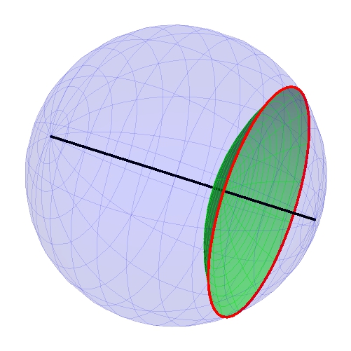
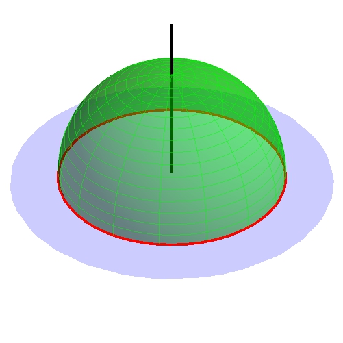
Figure 1: Hyperplane corresponding to the circular boundary at infinity. The hyperplane (the hypersurface of zero extrinsic curvature) reaches infinity at the circular boundary which divides infinity into two domains. The Poincaré spherical (left) and spherical half-space (right) representation of hyperbolic space is shown.

From a point of view of the conformally spherical geometry on ${{\mathcal{I}}}$, all such boundaries are equivalent. It is a reflection of the trivial fact that all hyperplanes in the bulk are isometric. Therefore we do not have any quantity measuring a ‘size’ of spherical boundaries at infinity.

However, in many calculations, both in the bulk or at infinity, we need to regularize various quantities. Instead of working at ${{\mathcal{I}}}$ we restrict on some cut-off surface at large finite size. Then we can measure the sizea of the circular boundaries using the geometry on the cut-off surface. But, since the choice of the cut-off can be rather arbitrary, the regularized size of the spherical boundary can be only an intermediate quantity, and physically measurable quantities should be cut-off independent.

Two circular boundaries can be in three qualitatively distinct positions: (i) disjoint boundaries (corresponding hyperplanes are ultraparallel), (ii) boundaries crossing each other (the hyperplanes intersect in a line), and (iii) boundaries touching in one point (the corresponding hyperplanes are asymptotic).

In the first case we can define the distance of the boundaries as a distance of the corresponding hyperplanes. To the crossing circular boundaries we can assign an angle of the corresponding hyperplanes. Finally, all pairs of touching boundaries are equivalent. Indeed, all pairs of asymptotic hyperplanes in an arbitrary position are isometric to each other. In global hyperbolic space there is no measure which could distinguish them.

Surface spanned on one boundary

Now we review known results for a minimal surface spanned on one circular boundary. Such a minimal surface is trivial: it is the hyperplane which defines the boundary. If we choose the axis of the cylindrical coordinates perpendicular to the hyperplane, the hyperplane is given by ${\zeta=\text{const}}$. If we choose the axis inside the hyperplane, the hyperplane is given by ${\varphi=\varphi_{0},\,\varphi_{0}+\pi}$. In the Poincaré coordinates the hyperplane is represented as a plane orthogonal to the infinity surface ${z=0}$ or as a hemisphere with the center at ${z=0}$ (here we used a language of the conformally related Euclidian geometry with Cartesian coordinates ${{\bar{x}},\,{\bar{y}},\,{\bar{z}}}$).

To demonstrate different regularizations used later, we can write down the area of a hyperplane measured up to a cut-off. For the hyperplane othogonal to the axis we have

$$A_{{\scriptstyle\mathrm{hp}}}=2\pi\ell^{2}(\sqrt{1+P^{2}}-1)=C\ell\Bigl{[}1-\frac{1}{P}+\mathcal{O}\Bigl{(}{\frac{1}{P^{2}}}\Bigr{)}\Bigr{]}\;,$$ (4)

where ${C=2\pi\ell P}$, with ${P=\operatorname{\mathrm{sh}}\rho_{*}}$, is the circumference of the circular boundary on the cut-off surface ${\rho=\rho_{*}\gg 1}$.

For the hyperplane which contains the axis we have

$$A_{{\scriptstyle\mathrm{hp}}}=2L\;\ell\sqrt{1-Z^{-2}}=2L\ell\Bigl{[}1+\mathcal{O}\Bigl{(}{\frac{1}{Z^{2}}}\Bigr{)}\Bigr{]}\;,$$ (5)

where ${L=Z\Delta\zeta_{*}\ell}$, with ${Z=\operatorname{\mathrm{ch}}\rho_{*}}$, is the length of the boundary at the cut-off surface. In this case, the circular boundary is represented by two lines ${\rho=\infty}$, ${\zeta\in{\mathbb{R}}}$, ${\varphi=\varphi_{0},\,\varphi_{0}+\pi}$. We thus have to introduce two cut-offs: an ultraviolet one, ${\rho=\rho_{*}}$, in the direction away from the axis, and an infrared one, ${\zeta=\pm\Delta\zeta_{*}/2}$, along the axis.

Finally, the area of the hyperplane represented by a half-plane in the Poincaré coordinates, say ${{\bar{x}}=\text{const}}$, is

$$A_{\scriptstyle\mathrm{hp}}=L\ell\;.$$ (6)

${L={\Delta{\bar{y}}_{*}}/{{\bar{z}}_{*}}}$ is again the length of the circular boundary at the cut-off surface ${{\bar{z}}={\bar{z}}_{*}\ll 1}$. It is also infrared divergent: one has to cut-off the ${{\bar{y}}}$ direction at ${{\bar{y}}=\pm\Delta{\bar{y}}_{*}/2}$.

In all three cases we recognize the well-known property that the leading diverging term of the minimal surface is (up to a constant scale) given by the regularized size of the boundary at infinity. Clearly, the exact expression for the divergent term depends on the regularization scheme, however, in all cases it can be interpreted as the regularized size of the boundary at infinity Hirata and Takayanagi (2007); Myers and Sinha (2011); Takayanagi (2012).

The area of the trivial minimal surface spanned on one circular boundary can be used to eliminate the infinite contributions to the area for more complicated surfaces. We define the renormalized area of a surface by subtracting the area of hyperplanes spanned on the same boundaries at infinity. In this sense, the trivial minimal surface has vanishing renormalized area.

Surfaces spanned on two boundaries

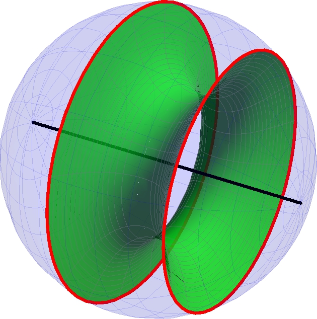
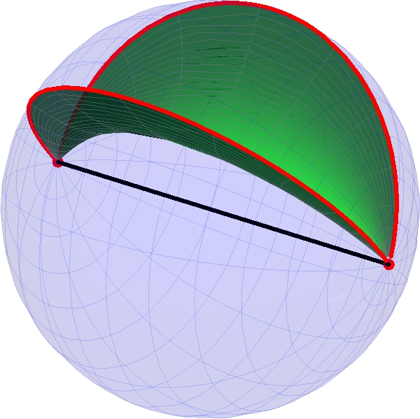
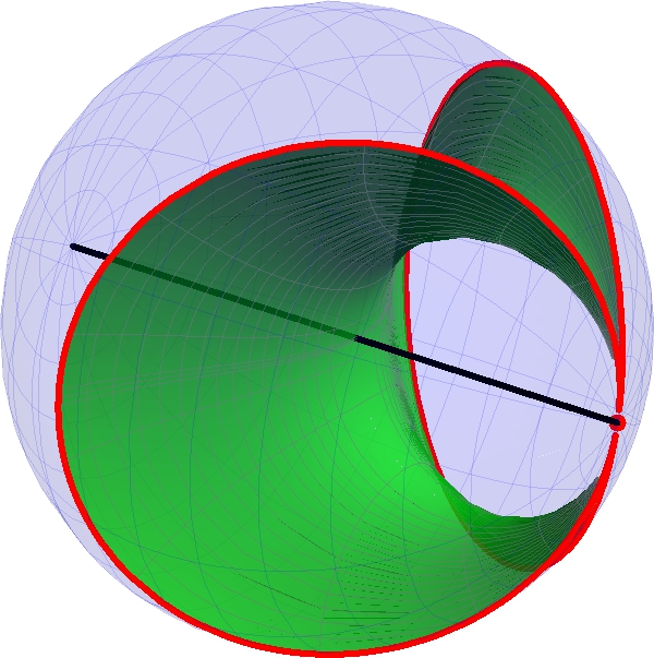
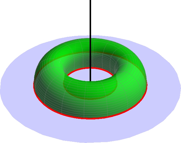
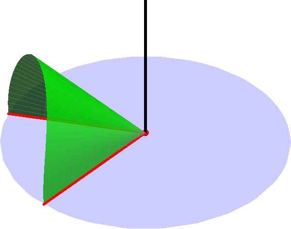
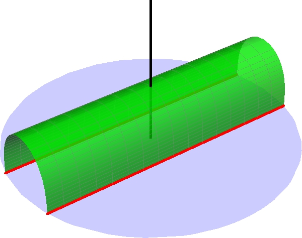
(a)                                                      (b)                                                      (c)

Figure 2: Minimal surfaces spanned on circular boundaries. The surfaces are visualized in Poincaré spherical (top) and Poincaré half-space (bottom) models. (a) The tube-like surface spanned on two disjoint boundaries. (b) The surface spanned on two semicircles joining opposite poles. (c) The surfaces spanned on two touching circles.

Disjoint boundaries. Given two circular boundaries at infinity, we can always find the unique line perpendicular to the corresponding hyperplanes in the bulk. If we adjust the cylindrical coordinates to this axis, the circular boundaries are represented by two circles ${\rho=\infty}$, ${\zeta=\pm\zeta_{\infty}}$. It is possible to find Krtouš and Zelnikov a tube-like minimal surface joining these two boundaries, see Fig. 2a. It is described by the function ${\zeta(P)}$ with ${P=\operatorname{\mathrm{ch}}\rho}$, and it is parametrized by ${P_{0}=\operatorname{\mathrm{ch}}\rho_{0}}$, where ${\rho_{0}}$ is the closest approach of the surface to the axis:

$$\begin{split}\zeta(P)&{=}\frac{\pm P_{0}}{\sqrt{1{+}P_{0}^{2}}\sqrt{1{+}2P_{0}^{2}}}\Bigl{[}(1{+}P_{0}^{2})\,\mathsf{F}\Bigl{(}{\textstyle\arccos\frac{P_{0}}{P},\sqrt{\frac{1+P_{0}^{2}}{1+2P_{0}^{2}}}}\Bigr{)}\\ &\mspace{60.0mu}-P_{0}^{2}\,\mathsf{\Pi}\Bigl{(}{\textstyle\arccos\frac{P_{0}}{P},\frac{1}{1+P_{0}^{2}},\sqrt{\frac{1+P_{0}^{2}}{1+2P_{0}^{2}}}}\Bigr{)}\Bigr{]}\;.\end{split}$$ (7)

Setting ${P=\infty}$ we can read out the coordinates ${\pm\zeta_{\infty}}$ of the circular boundaries:

$$\begin{split}&\zeta_{\infty}(P_{0})=\frac{P_{0}}{\sqrt{1+P_{0}^{2}}\sqrt{1+2P_{0}^{2}}}\\ &\quad\times\Bigl{[}(1+P_{0}^{2})\,\mathsf{K}\Bigl{(}{\textstyle\sqrt{\frac{1+P_{0}^{2}}{1+2P_{0}^{2}}}}\Bigr{)}-P_{0}^{2}\,\mathsf{\Pi}\Bigl{(}{\textstyle\frac{1}{1+P_{0}^{2}},\sqrt{\frac{1+P_{0}^{2}}{1+2P_{0}^{2}}}}\Bigr{)}\Bigr{]}\;.\end{split}$$ (8)

The distance between both boundaries, ${s=2\ell\zeta_{\infty}}$, as a function of the parameter ${P_{0}}$ is depicted in Fig. 3a. It reveals that the tube exists only for distances smaller than the maximal distance ${s_{\scriptstyle\mathrm{max}}\approx 1.00229\ell}$, and for these small distances there actually exist two tube-like minimal surfaces, one shallow one, remaining at large distances from the axis, and a deep one, approaching the axis. If the distance of circular boundaries is enlarged, the tube tears off and the minimal surface discontinuously splits into two trivial hyperplanes spanned on both boundaries.

To estimate which surface is the smallest one, we have to write down the regularized area:

$$\begin{split}A(P)&=\frac{4\pi\ell^{2}P_{0}^{2}}{\sqrt{1+2P_{0}^{2}}}\,\mathsf{\Pi}\Bigl{(}{\textstyle\arccos\frac{P_{0}}{P},1,\sqrt{\frac{1+P_{0}^{2}}{1+2P_{0}^{2}}}}\Bigr{)}\\ &=2A_{\scriptstyle\mathrm{hp}}+A_{\scriptstyle\mathrm{ren}}+\mathcal{O}\Bigl{(}\frac{1}{P^{3}}\Bigr{)}\;.\end{split}$$ (9)

The divergent term ${A_{\scriptstyle\mathrm{hp}}}$ is given by (4), the finite part ${A_{\scriptstyle\mathrm{ren}}}$ reads

$$\frac{A_{\scriptstyle\mathrm{ren}}}{4\pi\ell^{2}}={\textstyle 1{+}{\textstyle\frac{P_{0}^{2}}{\sqrt{1{+}2P_{0}^{2}}}}\mathsf{K}\Bigl{(}{\textstyle\!\sqrt{\frac{1{+}P_{0}^{2}}{1{+}2P_{0}^{2}}}}\Bigr{)}{-}\sqrt{1{+}2P_{0}^{2}}\,\mathsf{E}\Bigl{(}{\textstyle\!\sqrt{\!\frac{1{+}P_{0}^{2}}{1{+}2P_{0}^{2}}}}\Bigr{)}}\,.$$ (10)

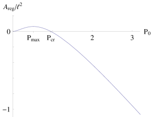
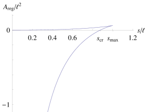
(a)                                                      (b)                                                      (c)

Figure 3: Renormalized area of the minimal surface spanned on two boundaries. (a) Relation between the distance ${s}$ of the boundaries and the closest approach ${P_{0}}$ of the tube to the axis. (b) Renormalized area of the tube as a function of ${P_{0}}$. (c) Renormalized area as a function of the distance ${s}$.

The renormalized area as a function of ${P_{0}}$ or of the distance ${s}$ is shown in Fig. 3. We see that the shallow tube has always smaller area than the deeper one. However, for ${s_{\scriptstyle\mathrm{cr}}<s<s_{\scriptstyle\mathrm{max}}}$, the renormalized area of the tube is positive, i.e., the tube has larger area than the trivial solutions of two hyperplanes. The tube is thus the smallest minimal surface only for ${s<s_{\scriptstyle\mathrm{cr}}\approx 0.876895\ell}$.

All these exact results confirm the previously conjectured properties based on numerical and approximate analysis Hirata and Takayanagi (2007).

Crossing circular boundaries. In the case of two crossing circular boundaries at infinity we naturally adjust the cylindrical coordinates to the axis going through the intersection points. Thus, the semicircles between these intersection points are represented by lines ${\rho=\infty}$, ${\varphi=\text{const}}$. In Poincaré coordinates they are half-lines in the plane ${{\bar{z}}=0}$ starting at ${{\bar{r}}=0}$. The minimal surface spanned on two such semicircles is depicted in Fig. 2b. Its explicit form can be found in Krtouš and Zelnikov . It exists for any angle ${\phi}$ between both semicircles and can be parametrized by ${Z_{0}=\operatorname{\mathrm{ch}}\rho_{0}}$ with ${\rho_{0}}$ corresponding to the closest approach of the surface to the axis. The relation between of ${\phi}$ and ${Z_{0}}$ is one-to-one Krtouš and Zelnikov . The regularized area takes form:

$$\begin{split}A(Z)&=\frac{2L\ell\,Z_{0}^{2}}{Z\sqrt{2Z_{0}^{2}-1}}\,\mathsf{\Pi}\Bigl{(}{\textstyle\arccos\frac{Z_{0}}{Z},1,\sqrt{\frac{Z_{0}^{2}-1}{2Z_{0}^{2}-1}}}\Bigr{)}\\ &=A_{\scriptstyle\mathrm{hp}}+\Delta\zeta_{*}\ell\Bigl{[}a_{\scriptstyle\mathrm{ren}}+\mathcal{O}\Bigl{(}\frac{1}{Z^{3}}\Bigr{)}\Bigr{]}\;.\end{split}$$ (11)

The leading term ${A_{\scriptstyle\mathrm{hp}}}$ is given by (5). It is divergent because of both UV and IR divergences. The next term is proportional to the IR cut-off ${\Delta\zeta_{*}}$. The reason is that the minimal surface is invariant under the translation along the axis. However, we can write down the finite renormalized area density ${a_{\scriptstyle\mathrm{ren}}=\frac{A_{\scriptstyle\mathrm{ren}}}{\Delta\zeta_{*}\ell}}$:

$$a_{\scriptstyle\mathrm{ren}}{=}2\ell\Bigl{[}{\textstyle\frac{Z_{0}^{2}}{\sqrt{2Z_{0}^{2}{-}1}}}\,\mathsf{K}\Bigl{(}{\textstyle\!\sqrt{\frac{Z_{0}^{2}{-}1}{2Z_{0}^{2}{-}1}}}\Bigr{)}{-}\sqrt{2Z_{0}^{2}{-}1}\,\mathsf{E}\Bigl{(}{\textstyle\!\sqrt{\frac{Z_{0}^{2}{-}1}{2Z_{0}^{2}{-}1}}}\Bigr{)}\Bigr{]}\,.$$ (12)

It is always negative. Naturally, the surface has always smaller area then two half-hyperplanes starting at the axis reaching the semi-circles at infinity.

Touching circular boundaries Tangent circular boundaries are trivially represented in Poincaré coordinates. If oriented in the ${{\bar{y}}}$ direction, they are given by ${{\bar{z}}=0}$, ${{\bar{x}}=\pm{\bar{x}}_{\infty}}$. The minimal surface spanned on such a ‘strip’ is in Fig. 2c, Tonni (2011); Krtouš and Zelnikov . It reaches the maximal value of the coordinate ${{\bar{z}}}$ for ${{\bar{z}}_{0}={\bar{x}}_{\infty}/X_{0}}$, which we call the ‘top-line’ of the surface. The constant ${X_{0}}$ is given by ${X_{0}=\frac{\Gamma(3/4)^{2}}{\sqrt{2\pi}}\approx 0.59907}$. The area regularized at ${{\bar{z}}\ll 1}$ is

$$\begin{split}A({\bar{z}})&=\frac{2\mathcal{A}\ell^{2}}{{\bar{z}}_{0}}\Biggl{[}\sqrt{\frac{{\bar{z}}_{0}^{2}}{{\bar{z}}^{2}}-\frac{{\bar{z}}^{2}}{{\bar{z}}_{0}^{2}}}-\sqrt{2}\,\mathsf{E}\Bigl{(}{\arccos\frac{{\bar{z}}}{{\bar{z}}_{0}},\frac{1}{\sqrt{2}}}\Bigr{)}\\ &\mspace{160.0mu}+\frac{1}{\sqrt{2}}\,\mathsf{F}\Bigl{(}{\arccos\frac{{\bar{z}}}{{\bar{z}}_{0}},\frac{1}{\sqrt{2}}}\Bigr{)}\Biggr{]}\\ &=A_{\scriptstyle\mathrm{hp}}+L_{0}\bigl{[}-2X_{0}\ell+O({\bar{z}}^{3})\bigr{]}\,.\end{split}$$ (13)

The leading divergent term ${A_{\scriptstyle\mathrm{hp}}}$ is given by (6). The next term is IR divergent since the surface has the horocyclic symmetry ${{\bar{y}}\to{\bar{y}}+{\bar{y}}_{s}}$. It is thus proportional to the length ${L_{0}=\frac{\Delta{\bar{y}}_{*}\ell}{{\bar{z}}_{0}}}$ measured on the ‘top-line’ of the surface. The renormalized area density ${a_{\scriptstyle\mathrm{ren}}}={\frac{A_{\scriptstyle\mathrm{ren}}}{L_{0}}}={-2X_{0}\ell}$ is, as expected, a constant independent of the position of the touching circular boundaries.

Discussion

Returning to the conjecture (2), we can now associate entanglement entropy with any two generally positioned spherical domains at infinity. The most interesting case occurs for two disjoint domains. For boundaries closer than ${s_{\scriptstyle\mathrm{max}}}$ there are three possible minimal surfaces, which corresponds to three possibilities (phases) for the holographic entanglement entropy in CFT. The physical choice would correspond to the surface of the smallest area. Inspecting Fig. 3b, one can see that the transition between these phases occurs at the distance ${s=s_{\scriptstyle\mathrm{cr}}}$, when the area of the tube-like surface starts to exceed the area of the trivial solution with two hyperplanes.

If we accept that the entanglement entropy for disjoint subsystems is given by the absolute minimal surface according to (2), then the renormalized area (10) is directly related to the mutual information ${I(\Omega_{1},\Omega_{2})=S_{\Omega_{1}}+S_{\Omega_{2}}-S_{\Omega_{1}\cup\Omega_{2}}}$ which quantifies correlations between the disjoint subsystems. Indeed, since the entanglement entropy ${S_{\Omega}}$ of a single spherical domain ${\Omega}$ is given by the area ${A_{\scriptstyle\mathrm{hp}}}$ of the trivial hyperplaneboundary ${\partial\Omega}$, , the renormalized area ${A_{\scriptstyle\mathrm{ren}}}$ of the tube joining the boundaries of two such domains gives directly the mutual information ${I(\Omega_{1},\Omega_{2})}$, provided that the tube does give the minimal area, i.e., for ${s<s_{\scriptstyle\mathrm{cr}}}$.

Although the entanglement entropy changes continuously with the distance between the boundaries at ${s=s_{\scriptstyle\mathrm{cr}}}$, the corresponding minimal surface changes discontinuously. To move from the trivial phase to the tube-like phase continuously, one would have to start with two very close hyperplanes. At a point, where they almost touch, a very deep tube-like surface can appear. By enlarging the distance of the boundaries, the tube starts to grow wider. It follows the upper branch of the curve in Fig. 3c (i.e. the non-physical phase) up to the maximal possible distance ${s_{\scriptstyle\mathrm{max}}}$ of the boundaries. Here, one has to start decreasing the distance of the boundaries in such a way that the tube grows even wider (following the lower branch in Fig. 3c). After decreasing the distance under ${s_{\scriptstyle\mathrm{cr}}}$ one obtains, in a continuous way, the physical tube-like phase.

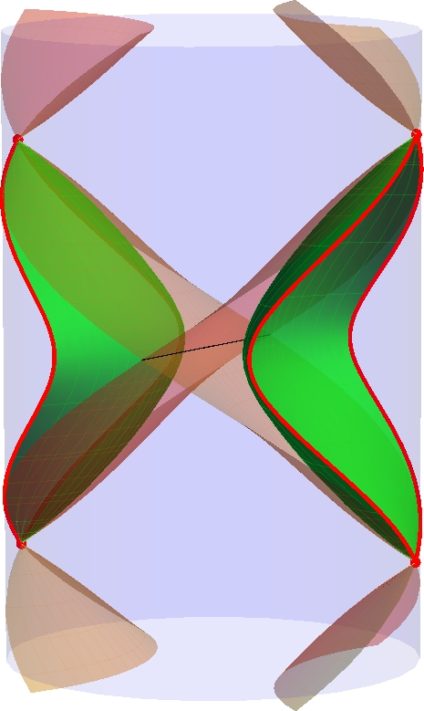
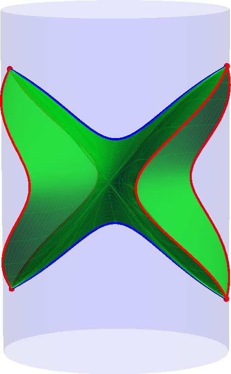
(a)                                       (b)

Figure 4: World-sheets of minimal surfaces. The vertical cylinder represents a 3+1 dimensional AdS spacetime with the angular direction ${\varphi}$ suppressed. The world-sheet of one circular boundary is thus reduced only to two curves at infinity. One circular boundary is localized in the left static region, the other in the right one. (a) Two uniformly accelerated hyperplanes spanned on these circular boundaries. Killing horizons are indicated. (b) The world-sheet of the tube-like minimal surface joining the same circular boundaries.

The fact that the tube-like minimal surface does not exist for too distant boundaries can be explored also in a dynamical way. Although we consider only static situations—calculation of the minimal surface area given in a spatial section of a static region of the AdS spacetime—we can take advantage of the rich structure of AdS symmetries and investigate the situation which looks rather dynamical in the global picture. Let us consider a static Killing vector with orbits that have an acceleration larger than ${1/\ell}$. This Killing vector has a bifurcation character similar to the boost Killing vector in the Minkowski spacetime. Its Killing horizons divide the AdS space into pairs of static regions positioned acausally with respect to each other, with non-static regions between, cf. Fig. 4a. The hyperbolic space in which we found the tube-like solution is a spatial section of both opposite static regions. We can position one circular boundary at infinity of one static region and the other one at infinity of the opposite static region. The world-sheets of the corresponding hyperplanes describe uniformly accelerated motion along the Killing vector, see Fig. 4a. The tube-like minimal surface can be also evolved into both static regions. However, it does reach the Killing horizons and there it must be extended into non-static regions. The resulting surface is depicted in Fig. 4b.

We see that the surface is non-smooth along two spatial edges, one describing the formation of the surface in the past, the other its termination in the future. If the surface is viewed from the perspective of a globally static observer (the vertical direction in the figure), the future edge can be interpreted as a tear-off line for the boundaries positioned too far from each other and the subsequent motion of the separate pieces. For more details, see Krtouš and Zelnikov .

Beside the case of two spherical domains we can investigate even more complicated situations: let us consider spherical domains ${\Omega_{i}}$, each of them a subdomain of all the subsequent ones: ${\Omega_{i}\subset\Omega_{j}}$ for ${i<j}$. They do not have to be all simultaneously concentric. The circular boundaries of these domains correspond to ultraparallel hyperplanes in the bulk. For such a configuration we know the minimal surfaces for any pair of the boundaries. Employing (2) we find that the renormalized entropy depends only on the distance of the boundaries, cf. (8), (9). We can thus test properties of the entropy for domains obtained by a combination of several subdomains. Namely, one can check the strong subadditivity inequalities to find that they are satisfied, as expected from general considerations Hirata and Takayanagi (2007).

Similarly one can study systems of strips between several semicircles joined at the same poles.

Summarizing, we have found exact analytical solutions for minimal surfaces in AdS for two disjoint domains at infinity. These classical geometrical solutions reveal the existence of different phases that reflect a phase transition in the corresponding quantum CFT, similar to the confinement/deconfinement phase transition at a finite temperature Klebanov et al. (2008); Lewkowycz (2012). The holographic entanglement entropy becomes an effective tool for testing phase transitions in CFT. Note that calculations in purely classical gravity provide an insight to non-trivial quantum properties of the corresponding field theories.

References

- Bekenstein (1972) J. Bekenstein, Lett. Nuovo Cim. 4, 737 (1972).
- Hawking (1972) S. Hawking, Commun. Math. Phys. 25, 152 (1972).
- Bombelli et al. (1986) L. Bombelli, R. K. Koul, J. Lee, and R. D. Sorkin, Phys. Rev. D 34, 373 (1986).
- Frolov and Novikov (1993) V. P. Frolov, I. Novikov, Phys. Rev. D 48, 4545 (1993), arXiv:gr-qc/9309001 [gr-qc].
- Srednicki (1993) M. Srednicki, Phys. Rev. Lett. 71, 666 (1993), arXiv:hep-th/9303048 [hep-th] .
- Barvinsky et al. (1995) A. Barvinsky, V. P. Frolov, and A. Zelnikov, Phys. Rev. D 51, 1741 (1995), arXiv:gr-qc/9404036 [gr-qc] .
- Susskind and Uglum (1994) L. Susskind and J. Uglum, Phys. Rev. D 50, 2700 (1994), arXiv:hep-th/9401070 [hep-th] .
- Sakharov (1968) A. Sakharov, Sov. Phys. Dokl. 12, 1040 (1968).
- Jacobson (1994) T. Jacobson, (1994), preprint, arXiv:gr-qc/9404039 [gr-qc] .
- Frolov et al. (1997a) V. P. Frolov, D. Fursaev, and A. Zelnikov, Nucl. Phys. B486, 339 (1997a), arXiv:hep-th/9607104 [hep-th] .
- Frolov et al. (1997b) V. P. Frolov, D. Fursaev, and A. Zelnikov, Nucl. Phys. Proc. Suppl. 57, 192 (1997b).
- Frolov et al. (2003) V. P. Frolov, D. Fursaev, and A. Zelnikov, JHEP 0303, 038 (2003), arXiv:hep-th/0302207 [hep-th] .
- Ryu and Takayanagi (2006a) S. Ryu and T. Takayanagi, Phys. Rev. Lett. 96, 181602 (2006a), arXiv:hep-th/0603001 [hep-th] .
- Ryu and Takayanagi (2006b) S. Ryu and T. Takayanagi, JHEP 0608, 045 (2006b), arXiv:hep-th/0605073 [hep-th] .
- Nishioka et al. (2009) T. Nishioka, S. Ryu, and T. Takayanagi, J. Phys. A42, 504008 (2009), arXiv:0905.0932 [hep-th] .
- Fursaev (2006) D. V. Fursaev, JHEP 0609, 018 (2006), arXiv:hep-th/0606184 [hep-th] .
- Hartman (2013) T. Hartman, (2013), preprint, arXiv:1303.6955 [hep-th] .
- Faulkner (2013) T. Faulkner, (2013), preprint, arXiv:1303.7221 [hep-th] .
- Lewkowycz and Maldacena (2013) A. Lewkowycz and J. Maldacena, JHEP 1308, 090 (2013), arXiv:1304.4926 [hep-th] .
- Faulkner et al. (2013) T. Faulkner, A. Lewkowycz, and J. Maldacena, (2013), preprint, arXiv:1307.2892 [hep-th] .
- Hung et al. (2011a) L.-Y. Hung, R. C. Myers, and M. Smolkin, JHEP 1104, 025 (2011a), arXiv:1101.5813 [hep-th] .
- Casini et al. (2011) H. Casini, M. Huerta, and R. C. Myers, JHEP 1105, 036 (2011), arXiv:1102.0440 [hep-th] .
- Myers et al. (2013) R. C. Myers, R. Pourhasan, and M. Smolkin, JHEP 1306, 013 (2013), arXiv:1304.2030 [hep-th] .
- Bhattacharyya et al. (2013) A. Bhattacharyya, A. Kaviraj, and A. Sinha, JHEP 1308, 012 (2013), arXiv:1305.6694 [hep-th] .
- Hung et al. (2011b) L.-Y. Hung, R. C. Myers, and M. Smolkin, JHEP 1108, 039 (2011b), arXiv:1105.6055 [hep-th] .
- Solodukhin (2011) S. N. Solodukhin, Living Rev. Rel. 14, 8 (2011), arXiv:1104.3712 [hep-th] .
- Klebanov et al. (2008) I. R. Klebanov, D. Kutasov, and A. Murugan, Nucl. Phys. B796, 274 (2008), arXiv:0709.2140 [hep-th] .
- Lewkowycz (2012) A. Lewkowycz, JHEP 1205, 032 (2012), arXiv:1204.0588 [hep-th] .
- Hirata and Takayanagi (2007) T. Hirata and T. Takayanagi, JHEP 0702, 042 (2007), arXiv:hep-th/0608213 [hep-th] .
- Headrick and Takayanagi (2007) M. Headrick and T. Takayanagi, Phys. Rev. D 76, 106013 (2007), arXiv:0704.3719 [hep-th] .
- Hubeny and Rangamani (2008) V. E. Hubeny and M. Rangamani, JHEP 0803, 006 (2008), arXiv:0711.4118 [hep-th] .
- (32) P. Krtouš and A. Zelnikov, “Minimal surfaces and entanglement entropy in anti-de Sitter space,” unpublished, in preparation.
- Myers and Sinha (2011) R. C. Myers and A. Sinha, JHEP 1101, 125 (2011), arXiv:1011.5819 [hep-th] .
- Takayanagi (2012) T. Takayanagi, Class. Quant. Grav. 29, 153001 (2012), arXiv:1204.2450 [gr-qc] .
- Gradshtein and Ryzhik (1994) I. S. Gradshtein and I. M. Ryzhik, Table of Integrals, Series, and Products (Academic Press, New York, 1994).
- Tonni (2011) E. Tonni, JHEP 1105, 004 (2011), arXiv:1011.0166 [hep-th] .