Investigating the Sharpe-Singleton scenario on the lattice by direct eigenvalue computation

Abstract:

We investigate the phase structure of lattice QCD with dynamical Wilson fermions. Wilson chiral perturbation theory predicts that the Aoki phase and the Sharpe-Singleton scenario manifest themselves in very distinct behavior of the Wilson Dirac eigenvalue spectrum. To test this prediction we perform a direct calculation of the eigenvalues of the non-Hermitian Wilson Dirac operator in dynamical lattice simulations. Moreover, we demonstrate an unexpected quark mass dependence on the shape of the eigenvalue distribution in the positive quark mass side.

1 Introduction

The study of the low-energy behavior of QCD is of considerable interest because of the open problem of spontaneous chiral symmetry breaking. While the low-energy regime lies outside of perturbation theory, there exists an effective field theory description for it, called Chiral Perturbation Theory. This effective theory offers a systematic way to compute, order by order in the quark mass and momenta, quantities of direct phenomenological importance. To further validate and verify predictions done using Chiral Perturbation Theory, one needs first principles calculations of QCD. At the moment this can only be done using the lattice formulation of QCD. Unfortunately, some lattice fermion formulations break chiral symmetry explicitly at nonzero lattice spacing. Moreover, the continuum limit, where one approaches zero lattice spacing, and the chiral limit, where one approaches zero quark mass, do not automatically commute. It is therefore imperative to have a good handle on the interplay between the symmetry breaking due to the discretization effects and due to the quark mass. The discretization effects depend on the lattice formulation and here we will focus on lattice simulations with Wilson fermions. In this case new phase structures, known as the Aoki phase [1] and the Sharpe-Singleton scenario [2], emerge if the continuum limit is taken prior to the chiral limit.

Since the discretization breaks chiral symmetry these effects can be included in Chiral Perturbation Theory. This extended effective theory is known as Wilson Chiral Perturbation Theory. To second order in the lattice spacing, three additional terms in the Lagrangian describe the discretization effects [2, 3, 4]. Each of these three terms comes with its own low-energy constant. Somewhat surprisingly, the sign of the constants are determined by the Hermiticity properties of the Wilson Dirac operator [5, 6, 7, 9]. The magnitude of the three new constants determines whether the Aoki phase or the Sharpe-Singleton scenario will be realized. Which scenario is realized in an actual lattice simulation depends on the detailed setup, including the coupling and clover coefficient.

The classic way to distinguish the Sharpe-Singleton scenario from the Aoki phase is by observing the pion mass as a function of quark mass [2]. In the Aoki phase the pion will be massless at a non-zero critical value of the quark mass, whereas in the Sharpe-Singleton scenario the pions are massive even with zero quark mass. To understand this lattice induced phase structure better it is most useful to consider the eigenvalue spectrum of the Wilson Dirac operator $D_{W}$: the second order transition into the Aoki phase (and hence the massless pions) occur precisely when the quark mass reaches the eigenvalue distribution of the Wilson Dirac operator, whereas the first order Sharpe-Singleton scenario is realized through a collective effect on the eigenvalue distributions induced by the quark mass [9]. Moreover, the distance from the quark mass to the eigenvalue spectrum acts as the effective quark mass which enters the standard form of the GOR relation [9]. The main purpose of this ongoing project is to test this eigenvalue realization of the phase structure of simulations with dynamical Wilson fermions. In particular, our aim is to observe the realization of the Sharpe-Singleton scenario through the collective behavior of the eigenvalues. We report here our current results for this project.

2 Wilson Chiral Perturbation Theory and the Sharpe-Singleton scenario

The Sharpe-Singleton scenario is realized through a collective jump of the eigenvalue distribution of the Wilson Dirac operator: for a positive quark mass, the eigenvalues form a band on the left side of the quark mass, and for a negative quark mass, the eigenvalues lie on the right side of the mass. Clearly, such a collective effect of the eigenvalues can only be induced by the quark mass in the unquenched theory. In contrast the quark mass only has a local effect on the Wilson Dirac eigenvalues in the Aoki phase.

This can be seen by calculating the two flavor eigenvalue density of $D_{W}$ using mean field Wilson chiral perturbation theory [9]

$$\rho_{c,N_{f}=2}^{MF}(\hat{x},\hat{m};\hat{a}_{6},\hat{a}_{8}) =\frac{1}{Z_{2}^{MF}(\hat{m};\hat{a}_{6},\hat{a}_{8})}$$ (1)

$$\times\bigg{\{}e^{2\hat{m}+16|\hat{a}^{2}_{6}|-4\hat{a}^{2}_{8}}\theta(8\hat{a}^{2}_{8}-|\hat{x}+16|\hat{a}_{6}|^{2}|)$$

$$+e^{-2\hat{m}+16|\hat{a}^{2}_{6}|-4\hat{a}^{2}_{8}}\theta(8\hat{a}^{2}_{8}-|\hat{x}-16|\hat{a}_{6}|^{2}|)$$

$$+\theta(8(\hat{a}^{2}_{8}+2\hat{a}^{2}_{6})-|\hat{m}|)\theta\left(8\hat{a}^{2}_{8}-\left|\hat{x}+\frac{2|\hat{a}_{6}|^{2}\hat{m}}{\hat{a}^{2}_{8}-2|\hat{a}_{6}|^{2}}\right|\right)e^{\hat{m}^{2}/8(\hat{a}^{2}_{8}-2|\hat{a}^{2}_{6}|)+4\hat{a}^{2}_{8}}\bigg{\}}.$$

Here the notation is as follows:

$$\hat{a}_{i}^{2}=a^{2}VW_{i},\;\hat{m}=mV\Sigma$$ (2)

where $W_{i}$ are the new low energy constants, $a$ is the lattice spacing, $m$ is the quark mass, $V$ is the system volume and $\Sigma$ is the chiral condensate. In the mean field limit considered here these dimensionless variables all have a magnitude much greater than unity.

The Sharpe-Singleton scenario is realized for $\hat{a}_{8}^{2}+2\hat{a}_{6}^{2}<0$. In this case, the effect of the quark mass changing sign can be seen by inspecting the contributions of the different terms in Eq. (1) on the eigenvalue density. The first term gives rise to a strip of eigenvalues centered at $-16|\hat{a}^{2}_{6}|/\Sigma$ of half width of $8\hat{a}_{8}^{2}/\Sigma$. The second term similarly gives rise to a strip of eigenvalues centered at $16|\hat{a}^{2}_{6}|/\Sigma$ with the same half width. Both of these terms have exponential suppression with differing signs of mass. Now, if the mass changes sign from $\hat{m}$ to $-\hat{m}$, the strip of eigenvalues at $-16|\hat{a}^{2}_{6}|/\Sigma$ jumps to $16|\hat{a}^{2}_{6}|/\Sigma$. This is sketched in Fig. 1, where on the left we have a positive quark mass and the distribution lies on the left of the quark mass, and on the right the quark mass is negative and the distribution is on the right of the quark mass.

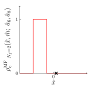
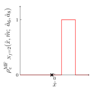
Figure 1: A sketch of the collective jump effect induced by a change in the quark mass sign in the Sharpe-Singleton scenario. The cross on the $x$-axis indicates the mass [9].

3 Numerical simulations

We simulated SU(3) with two flavours on a $V=12^{4}$ lattice with $\beta=5.47$. Our choice of the coupling corresponded to a lattice spacing of $a=0.16$ fm. We used Wilson fermions with clover improvement [10], setting $c_{SW}=1$, and we implemented one level of hypercubic smearing [11] on the gauge fields. We varied the bare quark mass $m_{0}$ in the range $m_{0}=-0.4\ldots 0.25.$

We calculated fifty of the lowest lying eigenvalues of the Wilson Dirac operator (sorted by the real part of the eigenvalues) from one hundred gauge field configurations per bare quark mass choice. The eigenvalues were calculated using our own parallelized implementation of the Arnoldi algorithm which is capable of running on GPUs. The numerical complexity of the eigenvalue calculation for a single configuration was of the order of $10^{15}$ FLOPs, which warranted using our own implementation over the industry standard ARPACK [12].

Our code implements the implicitly restarted Arnoldi method (IRAM), with deflation [13] and supports both MPI parallelization and CUDA. Employing techniques such as kernel fusion and custom kernels allowed us to implement the method with minimal memory requirements and double the performance of our initial version which was based on BLAS-like function calls. The parallelization framework used is based on work introduced in [14] and it allows us to write custom parallel kernels with complete abstraction of the architecture. The algorithm itself is – for the most part – memory bandwidth bound, and testing our code with a $16^{4}$ lattice on a Tesla K20m GPU shows that we reach 146 GB/s of effective bandwidth of the 175BG/s peak bandwidth (ECC on), meaning 83 percent of the theoretical maximum. This makes our code on the GPU run 18.5 times faster than ARPACK++ on one core of a Xeon X5650 @ 2.67GHz (32GB/s), measured by the time it took for each implementation to perform the same number of Arnoldi iterations. Scaling tests were performed using Tesla M2050 GPUs and the code was seen to scale well to local volumes as small as $8\times 8\times 16\times 16$ (4 GPUs) with at least a 70 percent increase for every doubling of compute resources and still a 40 percent increase when going from 4 to 8 GPUs. Here scaling stops due to the fact that the local volume for each GPU is too small to fill the whole processor for work. Our implementation of the algorithm is public and free to use.

We generated configurations with trajectory length of 1 for the positive axial quark mass configurations and calculated the eigenvalues every twentieth configurations. The integrator used was Omelyan 5 [15]. Similarly for the negative cases the trajectory length was 0.5 and the eigenvalues were calculated every fortieth configuration. This was because of the difficulty in simulating near zero axial quark mass, which required us to use conservative integrator time steps. Both our trajectory generation and the Arnoldi algorithm were run on up to six parallel GPUs using our GPU-capable parallel code [14]. Trajectory generation time ranged from around eighty seconds for positive quark masses to around five minutes for negative masses, although for half the trajectory length of the positive mass cases. The Arnoldi algorithm took around seven minutes per configuration.

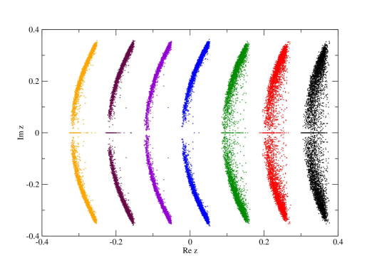
Figure 2: Scatterplot of the eigenvalues $D_{W}+m$ for different $m_{0}$. From right to left the bare quark mass values are $0.2,0.1,0.0,-0.1,-0.2,-0.3$ and $-0.4.$

The scatterplot in Fig. 2 shows the eigenvalues of $D_{W}+m$ for different values of the quark mass. We observe that with the current lattice setup the eigenvalue density does not show a collective jump across the origin. Moreover, the width of the eigenvalue distribution along the real axis as it passes zero is on the order of the smallest imaginary part of the eigenvalue. We conclude that the lattice effects in this simulation are so well under control that neither the Aoki nor the Sharpe-Singleton scenario is fully realized. We have computed the pion mass as a function of the quark mass in order to verify this. However, at the current lattice volume these measurements are somewhat delicate.

In mean field Wilson chiral perturbation theory to order $a^{2}$ the width of the eigenvalue distribution is independent of the quark mass, cf. Eq. (1). Unexpectedly, from this point of view, we observe a strong quark mass dependence in the shape of the distribution. The width of the distribution is seen being fairly constant in the negative axial quark mass side, whereas on the positive side it seems to grow with mass. One can also see in the figure that the zero axial quark mass is on the negative bare quark mass side, and that there is a notable depletion of real eigenvalues when one closes in on the zero axial quark mass.

In order to quantify this, we first calculated the variance in the real axis direction for each individual eigenvalue. We denoted the eigenvalues as ordered by their imaginary parts as
$z_{i}=x_{i}+iy_{i}$, with $0<y_{1}<y_{2}<\ldots<y_{n}$ and calculated the variance for each eigenvalue with $\sigma^{2}_{i}=\left<x_{i}^{2}\right>-\left<x_{i}\right>^{2}$. The results are shown in Fig. 3 for the smallest five of the eigenvalues calculated.

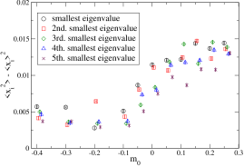
Figure 3: Variance in the real axis direction for individual eigenvalues for various bare quark masses.

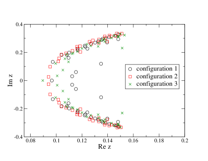
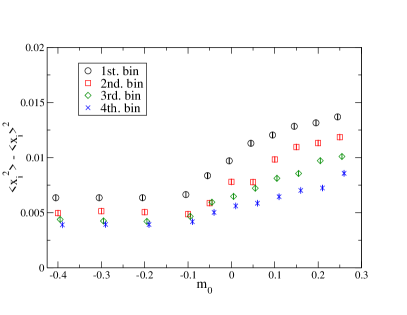
Figure 4: At left, a scatterplot of the eigenvalues calculated from three nonconsecutive configurations. At right, variance calculated by binning the eigenvalues.

Since the data seemed quite noisy, and because of the overlap between nearby eigenvalues configuration by configuration, we repeated the variance calculation by binning the eigenvalues into groups of five. The results of this procedure are shown in Fig. 4. It should be kept in mind that these results depend on both the number of eigenvalues calculated and the sorting criterion, but regardless of of them the mass dependence is clearly visible.

4 Conclusions

We are investigating the phase structure of lattice simulations with dynamical Wilson fermions from the perspective of the Wilson Dirac eigenvalues. The eigenvalues of the Wilson Dirac operator were computed with our own parallelized implementation of the Arnoldi algorithm. With our present lattice setup the lattice effects are so well under control that the eigenvalues at small mass behave almost as in the continuum. Hence, from the perspective of the Wilson Dirac eigenvalues, the simulations does not fully enter the Aoki phase nor does it fully realize the Sharpe-Singleton scenario. We are currently computing the spectrum of the Hermitian Wilson Dirac operator in order to verify this.

Our computations of the pion masses are somewhat delicate because of the limited lattice volume. However, with the parallelized implementation of the Arnoldi algorithm studies at larger volumes are also within our reach.

Finally, we have studied the shape of the eigenvalue distributions. Surprisingly from the point of view of Wilson chiral perturbation theory we demonstrated a strong mass dependence of this shape. We plan to test if this dependence persists in larger volumes. One possibility is that it is due to higher order terms in Wilson chiral perturbation theory, but at present no analytic predictions beyond order $a^{2}$ are available.

References

- [1] S. Aoki, Phys. Rev. D 30 (1984) 2653.
- [2] S. R. Sharpe and R. L. Singleton, Jr, Phys. Rev. D 58 (1998) 074501 [hep-lat/9804028].
- [3] O. Bar, G. Rupak and N. Shoresh, Phys. Rev. D 70 (2004) 034508 [hep-lat/0306021].
- [4] G. Rupak and N. Shoresh, Phys. Rev. D 66 (2002) 054503 [hep-lat/0201019].
- [5] P. H. Damgaard, K. Splittorff and J. J. M. Verbaarschot, Phys. Rev. Lett. 105 (2010) 162002 [arXiv:1001.2937 [hep-th]].
- [6] G. Akemann, P. H. Damgaard, K. Splittorff and J. J. M. Verbaarschot, Phys. Rev. D 83 (2011) 085014 [arXiv:1012.0752 [hep-lat]].
- [7] M. T. Hansen and S. R. Sharpe, Phys. Rev. D 85 (2012) 014503 [arXiv:1111.2404 [hep-lat]].
- [8] M. T. Hansen and S. R. Sharpe, Phys. Rev. D 85 (2012) 054504 [arXiv:1112.3998 [hep-lat]].
- [9] M. Kieburg, K. Splittorff and J. J. M. Verbaarschot, Phys. Rev. D 85 (2012) 094011 [arXiv:1202.0620 [hep-lat]].
- [10] K. Jansen and C. Liu, Comput. Phys. Commun. 99 (1997) 221.
- [11] A. Hasenfratz and F. Knechtli, Phys. Rev. D 64 (2001) 034504 [hep-lat/0103029].
- [12] R. B. Lehoucq, D. C. Sorensen and C. Yang, ARPACK Users’ Guide (SIAM, Philadelphia, 1998).
- [13] D. C. Sorensen, SIAM J. Matrix Anal. Appl. 17 (1996).
- [14] T. Rantalaiho, Porting production level quantum chromodynamics code to graphics processing units – a case study in Applied Parallel and Scientific Computing (Springer, Berlin, 2013).
- [15] I. P. Omelyan, I. M. Mryglod and R. Folk, Comput. Phys. Commun. 151 (2003) 272.