Antinucleon-nucleon interaction in chiral effective field theory

Abstract

Results of an exploratory study of the antinucleon-nucleon interaction within chiral effective field theory are reported. The antinucleon-nucleon potential is derived up to next-to-next-to-leading order, based on a modified Weinberg power counting, in close analogy to pertinent studies of the nucleon-nucleon interaction. The low-energy constants associated with the arising contact interactions are fixed by a fit to phase shifts and inelasticities provided by a recently published phase-shift analysis of antiproton-proton scattering data. The overall quality of the achieved description of the antinucleon-nucleon amplitudes is comparable to the one found in case of the nucleon-nucleon interaction at the same order. For most $S$-waves and several $P$-waves good agreement with the antinucleon-nucleon phase shifts and inelasticities is obtained up to laboratory energies of around 200 MeV.

1 Introduction

The antinucleon-nucleon ($\bar{N}N$) interaction has been studied quite extensively in the past Dover80 ; Dover82 ; Cote ; Timmers ; Hippchen ; Mulla ; Mull ; Entem06 ; Bennich , not least because of the wealth of data collected at the LEAR facility at CERN, cf. the reviews Rev1 ; Rev2 ; Rev3 . The majority of those investigations has been performed in the traditional meson-exchange framework where the $G$-parity transformation is exploited to connect the elastic part of the $\bar{N}N$ interaction with the dynamics in the nucleon-nucleon ($NN$) system. Annihilation processes are described either by a simple optical potential (which is often assumed to be spin- as well as energy-independent) Dover80 ; Dover82 ; Hippchen ; Mull or in terms of a coupling to a small number of effective two-body annihilation channels Cote ; Timmers ; Bennich .

In the last two decades chiral effective field theory (EFT) has become a standard tool in the studies of the $NN$ interaction at low energies. This developement was initiated by two seminal papers by Weinberg Wei90 ; Wei91 in which he proposed that EFT and the power-counting rules associated with it should be applied to the $NN$ potential rather than to the reaction amplitude. The reaction amplitude is then obtained from solving a regularized Lippmann-Schwinger equation for the derived interaction potential. His suggestion is based on the observation that diagrams with purely nucleonic intermediate states are strongly enhanced and, therefore, not amenable to a perturbative treatment. However, they can be taken into account and they are actually summed up to infinite order when solving the Lippmann-Schwinger equation. The chiral $NN$ potential contains pion exchanges and a series of contact interactions with an increasing number of derivatives. The latter represent the short-range part of the $NN$ force and are parametrized by low-energy constants (LECs), that need to be fixed by a fit to data. For reviews we refer the reader to the recent Refs. Epelbaum:2008ga ; Machleidt:2011zz . Presently the most refined calculations extend up to next-to-next-to-next-to-leading order (N³LO) Entem:2003ft ; Epe05 and they yield a rather accurate description of the $NN$ phase shifts up to laboratory energies of 250-300 MeV.

Naturally, the success of chiral EFT in the $NN$ sector provides a strong motivation to apply the same approach also to the $\bar{N}N$ interaction. First and most important for the practical implementation, recently an update of the Nijmegen partial-wave analysis (PWA) of antiproton-proton ($\bar{p}p$) scattering data Timmermans has been published. For the new PWA Zhou2012 the resulting phase shifts and inelasticities are explicitly given and can be readily used for applying the chiral EFT approach to the $\bar{N}N$ interaction in the very same way as it has been done for the $NN$ system.

A further incentive for exploring the feasibility of investigating the $\bar{N}N$ system within chiral EFT comes from the expected increase in interest in the $\bar{N}N$ interaction in the future due to the Facility for Antiproton and Ion Research (FAIR) in Darmstadt whose construction is finally on its way. Among the various project planned at this site is the PANDA experiment PANDA which aims to study the interactions between antiprotons and fixed target protons and nuclei in the momentum range of 1.5-15 GeV/c using the high energy storage ring HESR.

Finally, chiral EFT could be a very powerful tool to analyze data from recent measurements of the $\bar{p}p$ invariant mass in the decays of $J/\psi$, $B$ mesons, etc., and of the reaction $e^{+}e^{-}\to\bar{p}p$. In several of those reactions a near-threshold enhancement in the mass spectrum was found Bai ; Aubert ; Aubert1 ; BES12 and this enhancement could allow one to extract information on the $\bar{p}p$ interaction at very low energies BuggFSI ; Zou ; Sibirtsev05 ; Loiseau ; JH06 ; JH06a ; Entem ; Dedonder ; JH12 .

In the present paper we report on results of an exploratory study of the antinucleon-nucleon interaction within chiral EFT. In our application of chiral EFT to the $\bar{N}N$ interaction we follow exactly the approach used by Epelbaum et al. Epe05 ; Epe04 ; Epe04a in the $NN$ case. It is consistent with the scheme originally proposed by Weinberg except that one aims for an energy-independent representation of the chiral potential Epe98 . For the time being we restrict ourselves to an evaluation of the potential up to next–to–next–to–leading order (NNLO). At leading order (LO) the potential is given by one–pion exchange (OPE) and two contact terms without derivatives. At next–to–leading order (NLO) contributions from the leading two–pion exchange (TPE) diagrams as well as seven more contact operators arise. Finally, at NNLO one gets contributions from the subleading TPE with one insertion of dimension two pion–nucleon vertices. Once the potential is established it has to be inserted into a regularized scattering equation in order to obtain the reaction amplitude. For the regularization we follow again closely the procedure adopted by Epelbaum et al. Epe05 ; Epe04a and others Entem:2003ft , in their study of the $NN$ interaction and introduce a momentum-dependent exponential regulator function.

For investigations of the $\bar{N}N$ interaction within EFT based on other schemes see Refs. Chen2010 ; Chen2011 , where the Kaplan-Savage-Wise resummation scheme Kaplan is employed. These authors considered the $\bar{N}N$ interaction up to NLO. There have been also attempts to compute specific $\bar{p}p$ annihilation channels in chiral EFT Tarasov .

The present paper is structured as follows: The effective $\bar{N}N$ potential up to NNLO is described in Section 2. We start with a brief review of the underlying power counting and then provide explicit expressions for the contributions from pion exchange and for the contact terms. We also discuss how we treat the annihilation processes. Finally, we introduce the Lippmann-Schwinger equation that we solve and the parameterization of the S-matrix that we use. In Section 3 we indicate our fitting procedure and then we present the results achieved at NLO and at NNLO. Phase shifts and inelasticites for $S$-, $P$-, and $D$- waves, obtained from our EFT interaction, are displayed and compared with those of the $\bar{N}N$ phase-shift analysis. Furthermore, predictions for $S$-wave scattering lengths are given. A summary of our work and an outlook on future investigations is given in Section 4.

2 Chiral potential at next-to-next-to-leading order

The contributions to the $NN$ interaction up to NNLO are described in detail in Refs. Epe05 ; Epe04 ; Epe04a . The underlying power counting is given by (considering only connected diagrams)

$$\nu=2L+\sum_{i}\Delta_{i},\quad\Delta_{i}=d_{i}+\frac{n_{i}}{2}-2$$ (1)

where $L$ is the number of loops in the diagram, $d_{i}$ is the number of derivatives or pion mass insertions, and $n_{i}$ the number of internal nucleon fields at the vertex $i$ under consideration. The LO potential corresponds to $\nu=0$ and consists of two four-nucleon contact terms without derivatives and of one-pion exchange. There are no contributions at order $\nu=1$ due to requirements from parity conservation and time-reversal invariance. At NLO ($\nu=2$) seven new contact terms (with two derivatives) arise, together with loop contributions from (irreducible) two-pion exchange. Finally, at NNLO ($\nu=3$) there are additional contributions from two-pion exchange resulting from one insertion of dimension two pion-nucleon vertices, see e.g. Ref. Bernard:1995dp . The corresponding diagrams are summarized in Fig. 1.

The structure of the $\bar{N}N$ interaction is practically identical and, therefore, the potential given in Refs. Epe05 ; Epe04a can be adapted straightforwardly for the $\bar{N}N$ case. For the ease of the reader and also for defining our potential uniquely we provide the explicit expressions below.

Figure 1: Relevant diagrams up-to-and-including NNLO. Solid and dashed lines denote the antinucleon/nucleon and the pion, respectively. The square symbolizes a contact vertex with two derivatives or a subleading $\pi N$ vertex. The contributions at LO, NLO, and NNLO are displayed from top to bottom.

2.1 Pion exchange

In line with Epe05 we adopt the following expression for the one-pion exchange potential

$$V_{1\pi}(q)=\biggl{(}\frac{g_{A}}{2F_{\pi}}\biggr{)}^{2}\,\left(1-\frac{p^{2}+p^{\prime 2}}{2m^{2}}\right)\mbox{\boldmath$\tau$}_{1}\cdot\mbox{\boldmath$\tau$}_{2}\,\frac{\mbox{\boldmath$\sigma$}_{1}\cdot{\bf q}\,\mbox{\boldmath$\sigma$}_{2}\cdot{\bf q}}{{\bf q}^{2}+M_{\pi}^{2}}\ ,$$ (2)

where ${\bf q}={\bf p}^{\prime}-{\bf p}$ is the transferred momentum defined in terms of the final (${\bf p}^{\prime}$) and initial (${\bf p}$) center-of-mass momenta of the baryons (nucleon or antinucleon). Obviously here relativistic $1/m^{2}$ corrections to the static one-pion exchange potential have been taken into account. As in the work Epe05 we take the larger value $g_{A}=1.29$ instead of $g_{A}=1.26$ in order to account for the Goldberger–Treiman discrepancy. This value, together with the used $F_{\pi}=92.4$ MeV, implies the pion-nucleon coupling constant $g_{NN\pi}=13.1$ which is consistent with the empirical value obtained from $\pi N$ and $NN$ data deSwart ; Bugg and also with modern determinations utilizing the GMO sum rule Baru:2011bw . For the nucleon (antinucleon) and pion mass we use the isospin-averaged values $m=938.918$ MeV and $M_{\pi}=138.039$ MeV, respectively. Note that the contribution of one-pion exchange to the $\bar{N}N$ interaction is of opposite sign as that in the $NN$ case. This sign difference arises from transforming the $NN\pi$ vertex to the $\bar{N}\bar{N}\pi$ vertex via charge conjugation and a rotation in the isospin space and is commonly referred to as $G$-parity transformation.

The two-pion exchange potential calculated using spectral function regularization Epe05 is given at NLO by

$$V_{2\pi}^{(2)}(q)=\mbox{\boldmath$\tau$}_{1}\cdot\mbox{\boldmath$\tau$}_{2}\,V_{C}^{(2)}(q)+{\mbox{\boldmath$\sigma$}_{1}\cdot{\bf q}\,\mbox{\boldmath$\sigma$}_{2}\cdot{\bf q}}\,V_{T}^{(2)}(q)+{\mbox{\boldmath$\sigma$}_{1}\cdot\,\mbox{\boldmath$\sigma$}_{2}}\,V_{S}^{(2)}(q)~{},$$ (3)

where

$$V_{C}^{(2)}(q) = -\frac{1}{384\pi^{2}F_{\pi}^{4}}\,L^{\tilde{\Lambda}}(q)\,\biggl{\{}4M_{\pi}^{2}(5g_{A}^{4}-4g_{A}^{2}-1)+q^{2}(23g_{A}^{4}-10g_{A}^{2}-1)+\frac{48g_{A}^{4}M_{\pi}^{4}}{4M_{\pi}^{2}+q^{2}}\biggr{\}}~{},$$ (4)

$$V_{T}^{(2)}(q) = -\frac{1}{q^{2}}V_{S}^{(2)}(q)=-\frac{3g_{A}^{4}}{64\pi^{2}F_{\pi}^{4}}\,L^{\tilde{\Lambda}}(q)~{},$$

and at NNLO by

$$V_{2\pi}^{(3)}(q)=V_{C}^{(3)}(q)+\mbox{\boldmath$\tau$}_{1}\cdot\mbox{\boldmath$\tau$}_{2}\,{\mbox{\boldmath$\sigma$}_{1}\cdot{\bf q}\,\mbox{\boldmath$\sigma$}_{2}\cdot{\bf q}}\,V_{T}^{(3)}(q)+\mbox{\boldmath$\tau$}_{1}\cdot\mbox{\boldmath$\tau$}_{2}\,{\mbox{\boldmath$\sigma$}_{1}\cdot\,\mbox{\boldmath$\sigma$}_{2}}\,V_{S}^{(3)}(q)~{},$$ (5)

with

$$V_{C}^{(3)}(q) = -\frac{3g_{A}^{2}}{16\pi F_{\pi}^{4}}\biggl{\{}2M_{\pi}^{2}(2c_{1}-c_{3})-c_{3}q^{2}\biggr{\}}(2M_{\pi}^{2}+q^{2})A^{\tilde{\Lambda}}(q)~{},$$ (6)

$$V_{T}^{(3)}(q) = -\frac{1}{q^{2}}V_{S}^{(3)}(q)=-\frac{g_{A}^{2}}{32\pi F_{\pi}^{4}}\,c_{4}(4M_{\pi}^{2}+q^{2})A^{\tilde{\Lambda}}(q)\,.$$

The NLO and NNLO loop functions $L^{\tilde{\Lambda}}(q)$ and $A^{\tilde{\Lambda}}(q)$ are given by

$$L^{\tilde{\Lambda}}(q)=\theta(\tilde{\Lambda}-2M_{\pi})\,\frac{\omega}{2q}\,\ln\frac{\tilde{\Lambda}^{2}\omega^{2}+q^{2}s^{2}+2\tilde{\Lambda}q\omega s}{4M_{\pi}^{2}(\tilde{\Lambda}^{2}+q^{2})}~{},\quad\omega=\sqrt{q^{2}+4M_{\pi}^{2}}~{},\quad s=\sqrt{\tilde{\Lambda}^{2}-4M_{\pi}^{2}}\,,$$ (7)

and

$$A^{\tilde{\Lambda}}(q)=\theta(\tilde{\Lambda}-2M_{\pi})\,\frac{1}{2q}\,\arctan\frac{q(\tilde{\Lambda}-2M_{\pi})}{q^{2}+2\tilde{\Lambda}M_{\pi}}\,.$$ (8)

For the LECs $c_{1}$ and $c_{4}$ we adopt the central values from the $Q^{3}$–analysis of the $\pi N$ system Paul : $c_{1}=-0.81$ GeV^-1, $c_{4}=3.40$ GeV^-1. For the constant $c_{3}$ the value $c_{3}=-3.40$ GeV^-1 is used, which is on the lower side but still consistent with the results from Ref. Paul . Note that slightly different values are employed in the $\bar{N}N$ partial-wave analysis Zhou2012 , namely $c_{1}=-0.76$ GeV^-1, $c_{3}=-5.8$ GeV^-1 and $c_{4}=4.0$ GeV^-1. These values are also consistent with the recent determination in Krebs:2012yv .

2.2 Contact terms

The spin-dependence of the potentials due to the leading order contact terms is given by Epe00

$$V^{(0)}_{\bar{N}N} = C_{S}+C_{T}\,\mbox{\boldmath$\sigma$}_{1}\cdot\mbox{\boldmath$\sigma$}_{2}\,,$$ (9)

where the parameters $C_{S}$ and $C_{T}$ are low-energy constants (LECs) which need to be determined in a fit to data. At NLO, the spin- and momentum-dependence of the contact terms reads

$$V^{(2)}_{\bar{N}N} = C_{1}{\bf q}^{\,2}+C_{2}{\bf k}^{\,2}+(C_{3}{\bf q}^{\,2}+C_{4}{\bf k}^{\,2})\,\mbox{\boldmath$\sigma$}_{1}\cdot\mbox{\boldmath$\sigma$}_{2}+\frac{i}{2}C_{5}(\mbox{\boldmath$\sigma$}_{1}+\mbox{\boldmath$\sigma$}_{2})\cdot({\bf q}\times{\bf k})$$ (10)

$$+ C_{6}({\bf q}\cdot\mbox{\boldmath$\sigma$}_{1})({\bf q}\cdot\mbox{\boldmath$\sigma$}_{2})+C_{7}({\bf k}\cdot\mbox{\boldmath$\sigma$}_{1})({\bf k}\cdot\mbox{\boldmath$\sigma$}_{2})\ ,$$

where $C_{i}$ ($i=1,\dots,7$) are additional LECs. The average momentum ${\bf k}$ is defined by ${\bf k}=({\bf p}^{\prime}+{\bf p})/2$. When performing a partial-wave projection, these terms contribute to the two $S$–wave (${}^{1}S_{0}$, ${}^{3}S_{1}$) potentials, the four $P$–wave (${}^{1}P_{1}$, ${}^{3}P_{0}$, ${}^{3}P_{1}$, ${}^{3}P_{2}$) potentials, and the ${}^{3}S_{1}$-${}^{3}D_{1}$ transition potential in the following way Epe05 :

$$V(^{1}S_{0}) = {4\pi}\,(C_{S}-3C_{T})+\pi\,(4C_{1}+C_{2}-12C_{3}-3C_{4}-4C_{6}-C_{7})({p}^{2}+{p}^{\prime 2})\,$$ (11)

$$= \tilde{C}_{{}^{1}S_{0}}+{C}_{{}^{1}S_{0}}({p}^{2}+{p}^{\prime 2})\,,$$

$$V(^{3}S_{1}) = {4\pi}\,(C_{S}+C_{T})+\frac{\pi}{3}\,(12C_{1}+3C_{2}+12C_{3}+3C_{4}+4C_{6}+C_{7})({p}^{2}+{p}^{\prime 2})\,$$ (12)

$$= \tilde{C}_{{}^{3}S_{1}}+{C}_{{}^{3}S_{1}}({p}^{2}+{p}^{\prime 2})~{},$$

$$V(^{1}P_{1}) = \frac{2\pi}{3}\,(-4C_{1}+C_{2}+12C_{3}-3C_{4}+4C_{6}-C_{7})\,{p}\,{p}^{\prime}={C}_{{}^{1}P_{1}}\,{p}\,{p}^{\prime}\,,$$ (13)

$$V(^{3}P_{1}) = \frac{2\pi}{3}\,(-4C_{1}+C_{2}-4C_{3}+C_{4}+2C_{5}-8C_{6}+2C_{7})\,{p}\,{p}^{\prime}={C}_{{}^{3}P_{1}}\,{p}\,{p}^{\prime}\,,$$ (14)

$$V(^{3}P_{0}) = \frac{2\pi}{3}\,(-4C_{1}+C_{2}-4C_{3}+C_{4}+4C_{5}+12C_{6}-3C_{7})\,{p}\,{p}^{\prime}={C}_{{}^{3}P_{0}}\,{p}\,{p}^{\prime}\,,$$ (15)

$$V(^{3}P_{2}) = \frac{2\pi}{3}\,(-4C_{1}+C_{2}-4C_{3}+C_{4}-2C_{5})\,{p}\,{p}^{\prime}={C}_{{}^{3}P_{2}}\,{p}\,{p}^{\prime}\,,$$ (16)

$$V(^{3}D_{1}-\,^{3}S_{1}) = \frac{2\sqrt{2}\pi}{3}\,(4C_{6}+C_{7})\,{p^{\prime}}^{2}={C}_{{}^{3}S_{1}-\,^{3}D_{1}}\,{p^{\prime}}^{2}\equiv{C}_{\epsilon_{1}}\,{p^{\prime}}^{2}\,,$$ (17)

$$V(^{3}S_{1}-\,^{3}D_{1}) = \frac{2\sqrt{2}\pi}{3}\,(4C_{6}+C_{7})\,{p}^{2}={C}_{{}^{3}S_{1}-\,^{3}D_{1}}\,{p}^{2}\equiv{C}_{\epsilon_{1}}\,{p}^{2}\,,$$ (18)

with $p=|{\bf p}\,|$ and ${p}^{\prime}=|{\bf p}\,^{\prime}|$. There are no additional contact terms at NNLO.

Note that the Pauli principle is absent in case of the $\bar{N}N$ interaction. Accordingly, each partial wave that is allowed by angular momentum conservation occurs in the isospin $I=0$ and in the $I=1$ channel. Therefore, there are now twice as many contact terms as in $NN$.

The main new feature in the $\bar{N}N$ interaction is the presence of annihilation processes. The $\bar{N}N$ system annihilates into a multitude of $n\,\pi$ channels, where the decay to 4 to 6 pions is dominant in the low-energy region of $\bar{N}N$ scattering Rev1 . The threshold energy of those channels is in the order of 700 MeV while the $\bar{N}N$ threshold is at 1878 MeV. Therefore, one does not expect that annihilation introduces a new scale into the problem. Accordingly, there should be no need to modify the power counting when going from $NN$ to $\bar{N}N$ because the momenta associated with the annihilation channels should be, in average, much larger than those in the $\bar{N}N$ system itself. This conjecture is supported by the fact that phenomenological models of the $\bar{N}N$ interaction can describe the bulk properties of annihilation very well by simple energy-independent optical potentials of Woods-Saxon or Gaussian type Dover80 ; Dover82 ; Hippchen ; Mull . The ranges associated with those interactions are of the order of 1 fm or less. The above considerations suggest that annihilation processes are primarily tied to short-distance physics and, therefore, can be and should be simply incorporated into the contact terms which anyway are meant to parameterize effectively the short-range part of (elastic) $NN$ and/or $\bar{N}N$ scattering.

Nonetheless we want to emphasize that the above arguments are of pragmatical nature and not fundamental ones. There are definitely annihilation channels that open near the $\bar{N}N$ threshold. Specifically, there are indications that a sizeable part of the annihilation into multipion channels proceeds via two-meson doorway modes like $\bar{N}N\to\rho\rho\to 4\pi$ or $\bar{N}N\to f_{2}(1270)\omega\to 5\pi$, and some of those have nominal thresholds close to that of $\bar{N}N$ scattering. On the other hand, according to empirical information the actual branching ratios into individual two-body channels are typically of the order of 1% Mull only and, therefore, they do not have any noticeable impact on the description of the bulk properties of $\bar{N}N$ annihilation. In fact, all the two-body annihilation channels together – as far as they have been measured – yield only about 30% of the total annihilation cross section at the $\bar{N}N$ threshold which is a strong evidence for the dominance of annihilation into 3 or more (uncorrelated) pions.

The study of $\bar{N}N$ scattering in EFT in Refs. Chen2010 ; Chen2011 followed the above arguments and took into account annihilation by simply using complex LECs in Eqs. (11)-(18). However, this prescription has an unpleasant drawback – it does not allow one to impose sensible unitarity requirements on the resulting scattering amplitude. With unitarity requirements we mean a condition that guarantees that for each partial wave its contribution to the total cross section is larger than its contribution to the integrated elastic cross section. In case of strict two-body unitary like for $NN$ scattering below the pion production threshold these two quantities are, of course, identical.

Since we want an approach that manifestly fulfils unitarity constraints we treat annihilation in a different way. We start out from the observation that unitarity requires the $\bar{N}N$ annihilation potential to be of the form

$$V_{ann}=\sum_{X=2\pi,3\pi,...}V_{\bar{N}N\to X}G_{X}V_{X\to\bar{N}N}$$ (19)

where $X$ is the sum over all open annihilation channels, and $G_{X}$ is the propagator of the intermediate state $X$. Note that Eq. (19) is exact under the assumption that there is no interaction in and no transition between the various annihilation channels. Performing an expansion of $V_{\bar{N}N\to X}$ up to NNLO analoguous to the $\bar{N}N$ interaction and evaluating formally the sum and integral in Eq. (19) yields a contribution from the unitarity cut that can be written as

$$V^{L=0}_{ann}=-i\,(\tilde{C}_{{}^{1}S_{0}}^{a}+C_{{}^{1}S_{0}}^{a}p^{2})(\tilde{C}_{{}^{1}S_{0}}^{a}+C_{{}^{1}S_{0}}^{a}p^{\prime 2}),\ \ \ \ V^{L=1}_{ann}=-i\,(C_{\alpha}^{a})^{2}pp^{\prime},$$ (20)

where $\alpha$ stands for the ${}^{3}P_{0}$, ${}^{1}P_{1}$, ${}^{3}P_{1}$, and ${}^{3}P_{2}$ partial waves. For the coupled ${}^{3}S_{1}-^{3}D_{1}$ partial wave we get

$$V^{S\to S}_{ann} = -i\,(\tilde{C}_{{}^{3}S_{1}}^{a}+C_{{}^{3}S_{1}}^{a}p^{2})(\tilde{C}_{{}^{3}S_{1}}^{a}+C_{{}^{3}S_{1}}^{a}p^{\prime 2}),\ \ \ \ V^{S\to D}_{ann}=-i\,(\tilde{C}_{{}^{3}S_{1}}^{a}+C_{{}^{3}S_{1}}^{a}p^{2})\,C_{\epsilon_{1}}^{a}p^{\prime 2},$$

$$V^{D\to S}_{ann} = -i\,C_{\epsilon_{1}}^{a}p^{2}\,(\tilde{C}_{{}^{3}S_{1}}^{a}+C_{{}^{3}S_{1}}^{a}p^{\prime 2}),\ \ \ \ \ \ \ V^{D\to D}_{ann}=-i\,(C_{\epsilon_{1}}^{a})^{2}p^{2}p^{\prime 2}\ .$$ (21)

In those expressions the parameters $\tilde{C}^{a}$ and $C^{a}$ are real. Thus, for each partial wave we essentially recover the structure of the potential that follows from the contact terms considered above, with the same number of free parameters. However, in Eqs. (20)–(21) the sign of $V_{ann}$ as required by unitarity is already explicitly fixed and does not depend on the sign of the parameters $\tilde{C}^{a}$ and $C^{a}$ anymore. Moreover, and most importantly, we see that a term proportional to $p^{2}p^{\prime 2}$ arises in the $S$ waves at NLO and NNLO from unitarity constraints and it has to be included in order to make sure that unitarity is fulfilled at any energy.

Note that, in principle, there is also a contribution from the principal-value part of the integral in Eq. (19). However, it is real and, therefore, its structure is already accounted for by the standard LECs in Eqs. (11)–(18).

Finally we would like to add that in practice the treatment of annihilation via Eqs. (20)–(21) corresponds to the introduction of an effective two-body annihilation channel with a threshold significantly below the one of $\bar{N}N$ so that the center-of-mass momentum in the annihilation channel is already fairly large and its variation in the low-energy region of $\bar{N}N$ scattering considered by us is negligible.

2.3 Scattering equation

In the actual calculation a partial-wave projection of the interaction potentials is performed, as described in detail in Ref. Epe05 . The reaction amplitudes are obtained from the solution of a relativistic Lippmann-Schwinger (LS) equation:

$$T_{L^{\prime\prime}L^{\prime}}(p^{\prime\prime},p^{\prime};E_{q})=V_{L^{\prime\prime}L^{\prime}}(p^{\prime\prime},p^{\prime})+\sum_{L}\int_{0}^{\infty}\frac{dpp^{2}}{(2\pi)^{3}}\,V_{L^{\prime\prime}L}(p^{\prime\prime},p)\frac{1}{2E_{q}-2E_{p}+i0^{+}}T_{LL^{\prime}}(p,p^{\prime};E_{q}).$$

(22)

Here, $E_{q}=\sqrt{m^{2}+q^{2}}$, where $q$ is the on-shell momentum. Like in the $NN$ case we have either uncoupled spin-singlet and triplet waves (where $L^{\prime\prime}=L^{\prime}=L=J$) or coupled partial waves (where $L^{\prime\prime},L^{\prime},L=J-1,J+1$). We solve the LS equation in the isospin basis, i.e. for $I=0$ and $I=1$ separately, and we compare the resulting phase shifts with those in Ref. Zhou2012 that are likewise given in the isospin basis. It should be said, however, that for a comparison directly with data a more refined treatment is required. Then one should solve the LS equation in particle basis and consider the coupling between the $\bar{p}p$ and $\bar{n}n$ channels explicitly. In this case one can take into account the mass difference between $p$ ($\bar{p}$) and $n$ ($\bar{n}$) and, thereby, implement the fact that the physical thresholds of the $\bar{p}p$ and $\bar{n}n$ channels are separated by about 2.5 MeV, and also one can add the Coulomb interaction in the $\bar{p}p$ channel. The potential in the LS equation is cut off with a regulator function,

$$f^{\Lambda}(p^{\prime},p)=\exp\left[-\left(p^{\prime 6}+p^{6}\right)/\Lambda^{6}\right],$$ (23)

in order to remove high-energy components Epe05 . The cutoff values are chosen in the range $\Lambda=450$ – $600\,$MeV at NLO and $\Lambda=450$ – $650\,$MeV at NNLO, similar to what was used for chiral $NN$ potentials Epe05 ; Epe04a .

The relation between the $S$– and on–the–energy shell $T$–matrix is given by

$$S_{LL^{\prime}}(q)=\delta_{LL^{\prime}}-\frac{i}{8\pi^{2}}\,q\,E_{q}\,T_{LL^{\prime}}(q)~{}.$$ (24)

The phase shifts in the uncoupled cases can be obtained from the $S$–matrix via

$$S_{LL}\equiv S_{L}=e^{2i\delta_{L}}\,.$$ (25)

For the $S$–matrix in the coupled channels ($J>0$) we use the so–called Stapp parametrization Stapp

$$\left(\begin{array}[]{cc}S_{J-1\,J-1}&S_{J-1\,J+1}\\ S_{J+1\,J-1}&S_{J+1\,J+1}\end{array}\right)=\left(\begin{array}[]{cc}\cos{2\epsilon_{J}}\,e^{2i\delta_{J-1}}&-i\sin{2\epsilon_{J}}\,e^{i(\delta_{J-1}+\delta_{J+1})}\\ -i\sin{2\epsilon_{J}}\,e^{i(\delta_{J-1}+\delta_{J+1})}&\cos{2\epsilon_{J}}\,e^{2i\delta_{J+1}}\end{array}\right)~{}.$$ (30)

In case of elastic scattering the phase parameters in Eqs. (25) and (30) are real quantities while in the presence of inelasticites they become complex. Because of that, in the past several generalizations of these formulae have been proposed that still allow one to write the $S$-matrix in terms of real parameters Arndt ; Zhou2012 . We follow here Ref. Bystricky and calculate and present simply the real and imaginary parts of the phase shifts and the mixing parameters obtained via the above parameterization. Note that with this choice the real part of the phase shifts is identical to the phase shifts one obtains from another popular parameterization where the imaginary part is written in terms of an inelasticity parameter $\eta$, e.g. for uncoupled partial waves

$$S_{L}=\eta e^{2i\delta_{L}}\;.$$ (31)

Indeed, for this case ${\rm Im}\,\delta_{L}=-(\log\eta)/2$ which implies that ${\rm Im}\,\delta_{L}\geq 0$ since $\eta\leq 1$ because of unitarity. Since our calculation implements unitarity, the optical theorem

$${\rm Im}\,a_{LL}(q)\geq q\,\sum_{L^{\prime}}|a_{LL^{\prime}}(q)|^{2}\ ,$$ (32)

is fulfilled for each partial wave, where $a_{LL^{\prime}}(q)=(S_{LL^{\prime}}-\delta_{LL^{\prime}})/2iq=-1/(4\pi)^{2}\,E_{q}\,T_{LL^{\prime}}(q)$.

For the fitting procedure and for the comparison of our results with those by Zhou and Timmermans we reconstructed the $S$-matrix based on the phase shifts listed in Tables VIII-X in Ref. Zhou2012 and on the formulae presented in Sect. VII of that paper and then converted them to our convention specified in Eqs. (25) and (30).

3 Results

In the fitting procedure we follow very closely the strategy of Epelbaum et al. in their study of the $NN$ interaction Epe05 ; Epe04a . In particular, we consider the same ranges for the cutoffs, namely for the cutoff in the LS equation values of $\Lambda$ = 450–600 MeV at NLO and $\Lambda$ = 450–650 MeV at NNLO while for the spectral function regularization variations we consider values in the range $\tilde{\Lambda}$ = 500–700 MeV. For any combination of the cutoffs $\Lambda$ and $\tilde{\Lambda}$, the LECs $C_{S,T}$ and $C_{1\ldots 7}$ are fixed from a fit to the $\bar{N}N$ $S$- and $P$-waves and the mixing parameter $\epsilon_{1}$ of Ref. Zhou2012 for laboratory energies below 125 MeV ($p_{lab}\leq 500$ MeV/c). The numerical values of the LECs are compiled in Tables 1 (NLO) and 2 (NNLO) for a selected combination of the cutoffs. The values for $\tilde{C}_{{}^{1}S_{0}}$ in the isospin $I=1$ case found in the fitting procedure turned out to be very small and, therefore, we set them to zero.

Our results are displayed and compared with the $\bar{N}N$ PWA Zhou2012 in Figs. 2-6. The bands represent the variation of the obtained phase shifts and mixing parameters with the cutoff. Those variations can be viewed as an estimate for the theoretical uncertainty. Thus, in principle for the same variation of the cutoff those bands should become narrower and narrower when one goes to higher order. However, as argued in Ref. Epe04a , in practice one has to be careful in the interpretation of the bands, specifically for the transition from NLO to NNLO. Since the same number of contact terms are present in the interactions at NLO and NNLO one rather should expect variations of similar magnitude. In particular, for reasons discussed in Epe04a the cutoff variation underestimates the uncertainty for the NLO results. In any case one has to keep in mind that, following Ref. Epe04a , we use a larger cutoff region at NNLO than for the NLO case.

Let us now discuss the individual partial waves. Results for the ${}^{1}S_{0}$ channel can be found in the upper part of Fig. 2. Obviously, the phase shift for isospin $I=0$ (we use here the spectral notation ${}^{(2I+1)(2S+1)}L_{J}$) is very well described up to fairly high energies – even at NLO – and likewise the inelasticity, presented in terms of the imaginary part of the phase shift. Moreover, the dependence on the cutoff is very small. In the $I=1$ channel the situation is rather different. Here we observe a sizeable cutoff dependence of the results for energy above 150 MeV. This has to do with the fact that the PWA suggests a resonance-like behavior of the phase in this region. Since this resonance lies in an energy region where we expect our results to show increasing uncertainties, based on the experience from the $NN$ case Epe04a , it is not surprising that it is difficult to reproduce this structure quantitatively. Nevertheless, there is a visible improvement when going from NLO to NNLO and at the latter order the empirical phase shifts already lie within the error bands of theory.

LEC		$\{450,\;500\}$	$\{600,\;500\}$	$\{450,\;700\}$	$\{600,\;700\}$
$I=0$	$\tilde{C}_{{}^{1}S_{0}}$	$-0.151$	$-0.267$	$-0.151$	$-0.273$
	$C_{{}^{1}S_{0}}$	$0.455$	$0.436$	$0.454$	$0.426$
	$\tilde{C}^{a}_{{}^{1}S_{0}}$	$0.270$	$0.232$	$0.232$	$0.177$
	$C^{a}_{{}^{1}S_{0}}$	$-0.915$	$-0.277$	$-0.905$	$-0.206$
	$C_{{}^{3}P_{0}}$	$1.150$	$1.453$	$1.398$	$1.724$
	$C^{a}_{{}^{3}P_{0}}$	$0.769$	$0.478$	$0.754$	$0.455$
$I=1$	$\tilde{C}_{{}^{1}S_{0}}$	$0$	$0$	$0$	$0$
	$C_{{}^{1}S_{0}}$	$0.446$	$0.692$	$0.449$	$0.675$
	$\tilde{C}^{a}_{{}^{1}S_{0}}$	$1.329$	$2.108$	$1.460$	$2.202$
	$C^{a}_{{}^{1}S_{0}}$	$-1.118$	$-0.369$	$-1.214$	$-0.498$
	$C_{{}^{3}P_{0}}$	$-0.357$	$-0.074$	$-0.321$	$0.041$
	$C^{a}_{{}^{3}P_{0}}$	$0.501$	$0.232$	$0.498$	$0.222$
$I=0$	$C_{{}^{1}P_{1}}$	$0.384$	$-0.015$	$0.394$	$0.020$
	$C^{a}_{{}^{1}P_{1}}$	$0.711$	$0.714$	$0.709$	$0.705$
	$C_{{}^{3}P_{1}}$	$-0.374$	$-0.235$	$-0.296$	$-0.146$
	$C^{a}_{{}^{3}P_{1}}$	$0.381$	$0.190$	$0.378$	$0.194$
	$\tilde{C}_{{}^{3}S_{1}}$	$-0.132$	$-0.083$	$-0.122$	$-0.075$
	$C_{{}^{3}S_{1}}$	$-0.497$	$-0.623$	$-0.731$	$-0.853$
	$\tilde{C}^{a}_{{}^{3}S_{1}}$	$0.334$	$0.325$	$0.319$	$0.301$
	$C^{a}_{{}^{3}S_{1}}$	$0.221$	$-0.573$	$0.325$	$-0.438$
	$C_{\epsilon_{1}}$	$0.496$	$0.520$	$0.557$	$0.585$
	$C^{a}_{\epsilon_{1}}$	$-0.599$	$-0.218$	$-0.653$	$-0.290$
$I=1$	$C_{{}^{1}P_{1}}$	$-0.623$	$-0.735$	$-0.659$	$-0.858$
	$C^{a}_{{}^{1}P_{1}}$	$0.682$	$0.544$	$0.688$	$0.573$
	$C_{{}^{3}P_{1}}$	$-0.180$	$-0.373$	$-0.201$	$-0.443$
	$C^{a}_{{}^{3}P_{1}}$	$0.716$	$0.628$	$0.719$	$0.645$
	$\tilde{C}_{{}^{3}S_{1}}$	$-0.089$	$-0.120$	$-0.087$	$-0.122$
	$C_{{}^{3}S_{1}}$	$0.698$	$0.148$	$0.707$	$0.188$
	$\tilde{C}^{a}_{{}^{3}S_{1}}$	$0.399$	$0.210$	$0.398$	$0.224$
	$C^{a}_{{}^{3}S_{1}}$	$0.164$	$0.665$	$0.124$	$0.602$
	$C_{\epsilon_{1}}$	$0.245$	$0.182$	$0.279$	$0.237$
	$C^{a}_{\epsilon_{1}}$	$0.015$	$0.111$	$-0.019$	$-0.046$
$I=0$	$C_{{}^{3}P_{2}}$	$0.225$	$0.466$	$0.363$	$0.630$
	$C^{a}_{{}^{3}P_{2}}$	$0.674$	$0.428$	$0.661$	$0.410$
$I=1$	$C_{{}^{3}P_{2}}$	$-0.362$	$-0.268$	$-0.361$	$-0.266$
	$C^{a}_{{}^{3}P_{2}}$	$0.528$	$0.350$	$0.529$	$0.351$

Table 1: The LECs at NLO for the different cutoff combinations $\big{\{}\Lambda\,[\mbox{MeV}],\;\tilde{\Lambda}\,[\mbox{MeV}]\big{\}}$. The values of the $\tilde{C}_{i}$ are in unit of $10^{4}$ GeV^-2 and the $C_{i}$ in $10^{4}$ GeV^-4. The parameters related to annihilation, $\tilde{C}^{a}_{i}$ and $C^{a}_{i}$ (see Eqs. (20)–(21)), are in units of $10^{2}$ GeV^-1 and $10^{2}$ GeV^-3, respectively.

LEC		$\{450,\;500\}$	$\{650,\;500\}$	$\{450,\;700\}$	$\{650,\;700\}$
$I=0$	$\tilde{C}_{{}^{1}S_{0}}$	$-0.140$	$-0.278$	$-0.141$	$-0.299$
	$C_{{}^{1}S_{0}}$	$0.456$	$0.459$	$0.456$	$0.463$
	$\tilde{C}^{a}_{{}^{1}S_{0}}$	$0.208$	$0.247$	$0.155$	$0.219$
	$C^{a}_{{}^{1}S_{0}}$	$-1.063$	$-0.337$	$-1.045$	$-0.233$
	$C_{{}^{3}P_{0}}$	$0.031$	$0.310$	$-0.444$	$-0.217$
	$C^{a}_{{}^{3}P_{0}}$	$0.796$	$0.492$	$0.828$	$0.556$
$I=1$	$\tilde{C}_{{}^{1}S_{0}}$	$0.025$	$0.095$	$0.052$	$-0.011$
	$C_{{}^{1}S_{0}}$	$0.453$	$0.213$	$0.450$	$0.189$
	$\tilde{C}^{a}_{{}^{1}S_{0}}$	$1.884$	$2.483$	$2.129$	$3.847$
	$C^{a}_{{}^{1}S_{0}}$	$-1.733$	$-2.778$	$-2.566$	$-4.474$
	$C_{{}^{3}P_{0}}$	$-0.535$	$-0.117$	$-0.531$	$-0.116$
	$C^{a}_{{}^{3}P_{0}}$	$0.514$	$0.182$	$0.517$	$0.182$
$I=0$	$C_{{}^{1}P_{1}}$	$0.400$	$-0.113$	$0.438$	$-0.069$
	$C^{a}_{{}^{1}P_{1}}$	$0.722$	$0.637$	$0.721$	$0.634$
	$C_{{}^{3}P_{1}}$	$-0.521$	$-0.339$	$-0.596$	$-0.432$
	$C^{a}_{{}^{3}P_{1}}$	$0.417$	$0.168$	$0.421$	$0.175$
	$\tilde{C}_{{}^{3}S_{1}}$	$-0.162$	$-0.100$	$-0.183$	$-0.103$
	$C_{{}^{3}S_{1}}$	$0.353$	$0.204$	$0.728$	$0.526$
	$\tilde{C}^{a}_{{}^{3}S_{1}}$	$0.364$	$0.371$	$0.397$	$0.415$
	$C^{a}_{{}^{3}S_{1}}$	$0.087$	$-0.841$	$-0.117$	$-1.125$
	$C_{\epsilon_{1}}$	$0.205$	$0.236$	$0.062$	$0.106$
	$C^{a}_{\epsilon_{1}}$	$-0.485$	$-0.002$	$-0.362$	$0.167$
$I=1$	$C_{{}^{1}P_{1}}$	$-1.013$	$-1.294$	$-1.349$	$-1.869$
	$C^{a}_{{}^{1}P_{1}}$	$0.711$	$0.535$	$0.775$	$0.668$
	$C_{{}^{3}P_{1}}$	$-0.530$	$-0.902$	$-0.794$	$-1.356$
	$C^{a}_{{}^{3}P_{1}}$	$0.742$	$0.630$	$0.788$	$0.735$
	$\tilde{C}_{{}^{3}S_{1}}$	$-0.067$	$-0.143$	$-0.044$	$-0.125$
	$C_{{}^{3}S_{1}}$	$1.150$	$0.764$	$1.325$	$1.235$
	$\tilde{C}^{a}_{{}^{3}S_{1}}$	$0.413$	$0.282$	$0.411$	$0.402$
	$C^{a}_{{}^{3}S_{1}}$	$-0.336$	$0.211$	$-0.896$	$-0.441$
	$C_{\epsilon_{1}}$	$0.320$	$0.287$	$0.376$	$0.383$
	$C^{a}_{\epsilon_{1}}$	$-0.065$	$0.021$	$-0.182$	$-0.162$
$I=0$	$C_{{}^{3}P_{2}}$	$-0.300$	$-0.120$	$-0.518$	$-0.399$
	$C^{a}_{{}^{3}P_{2}}$	$0.707$	$0.402$	$0.731$	$0.443$
$I=1$	$C_{{}^{3}P_{2}}$	$-0.648$	$-0.558$	$-0.821$	$-0.782$
	$C^{a}_{{}^{3}P_{2}}$	$0.544$	$0.329$	$0.565$	$0.377$

Table 2: The LECs at NNLO for the different cutoff combinations $\big{\{}\Lambda\,[\mbox{MeV}],\;\tilde{\Lambda}\,[\mbox{MeV}]\big{\}}$. The values of the $\tilde{C}_{i}$ are in unit of $10^{4}$ GeV^-2 and the $C_{i}$ in $10^{4}$ GeV^-4. The parameters related to annihilation, $\tilde{C}^{a}_{i}$ and $C^{a}_{i}$ (see Eqs. (20)–(21)), are in units of $10^{2}$ GeV^-1 and $10^{2}$ GeV^-3, respectively.

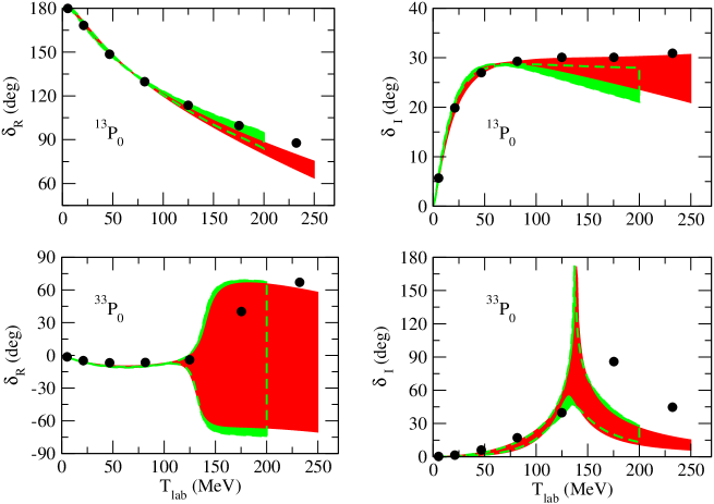
Figure 2: Real and imaginary parts of the phase shift in the ${}^{1}S_{0}$ and ${}^{3}P_{0}$ partial waves. The red/dark band shows the chiral EFT results up to NNLO for variations of the cutoff in the range $\Lambda=$ 450–650 MeV in the Lippmann-Schwinger equation, while the green/light band are results to NLO for $\Lambda=$ 450–600 MeV. The cutoff in the pion loops is varied independently in the range $\tilde{\Lambda}=$ 500–700 MeV. The solid circles represent the solution of the PWA of Ref. Zhou2012 .

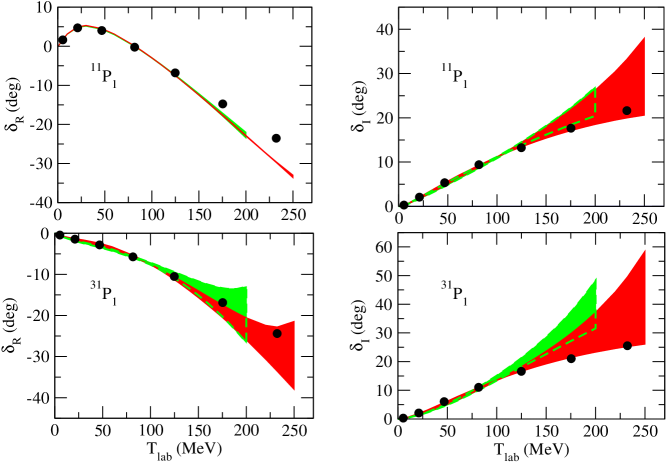
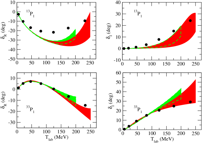
Figure 3: Real and imaginary parts of the phase shift in the ${}^{1}P_{1}$ and ${}^{3}P_{1}$ partial waves. The red/dark band shows the chiral EFT results up to NNLO for variations of the cutoff in the range $\Lambda=$ 450–650 MeV in the Lippmann-Schwinger equation, while the green/light band are results to NLO for $\Lambda=$ 450–600 MeV. The cutoff in the pion loops is varied independently in the range $\tilde{\Lambda}=$ 500–700 MeV. The solid circles represent the solution of the PWA of Ref. Zhou2012 .

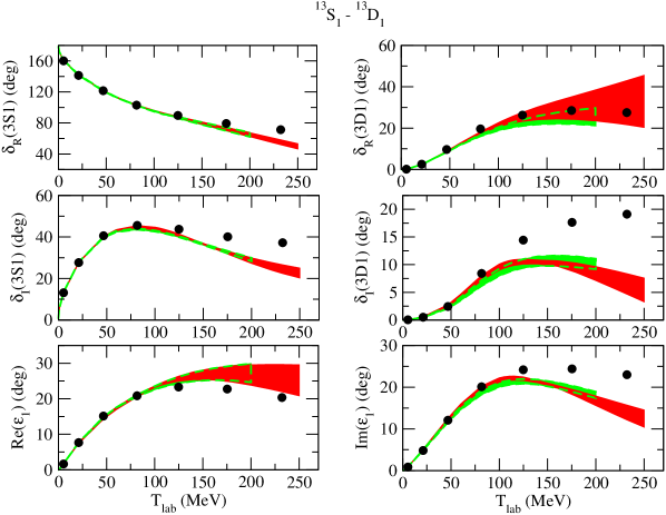
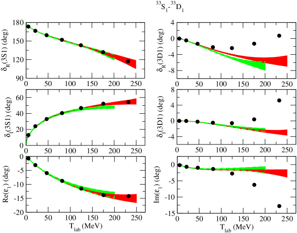
Figure 4: Real and imaginary parts of the phase shift in the ${}^{3}S_{1}$–${}^{3}D_{1}$ partial wave. The red/dark band shows the chiral EFT results up to NNLO for variations of the cutoff in the range $\Lambda=$ 450–650 MeV in the Lippmann-Schwinger equation, while the green/light band are results to NLO for $\Lambda=$ 450–600 MeV. The cutoff in the pion loops is varied independently in the range $\tilde{\Lambda}=$ 500–700 MeV. The solid circles represent the solution of the PWA of Ref. Zhou2012 .

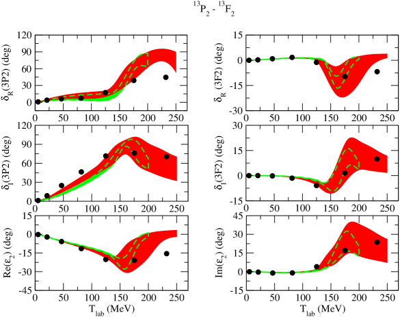
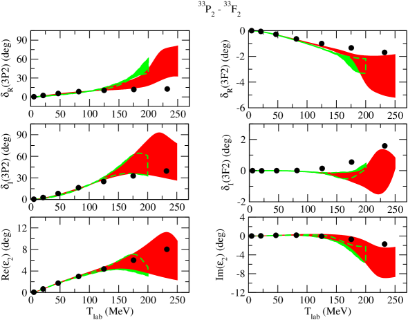
Figure 5: Real and imaginary parts of the phase shift in the ${}^{3}P_{2}$–${}^{3}F_{2}$ partial wave. The red/dark band shows the chiral EFT results up to NNLO for variations of the cutoff in the range $\Lambda=$ 450–650 MeV in the Lippmann-Schwinger equation, while the green/light band are results to NLO for $\Lambda=$ 450–600 MeV. The cutoff in the pion loops is varied independently in the range $\tilde{\Lambda}=$ 500–700 MeV. The solid circles represent the solution of the PWA of Ref. Zhou2012 .

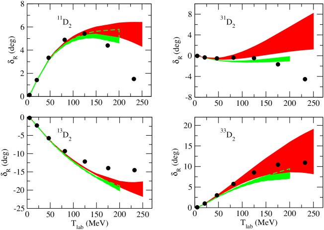
Figure 6: Real part of the phase shift in the ${}^{1}D_{2}$ and ${}^{3}D_{2}$ partial waves. The red/dark band shows the chiral EFT results up to NNLO for variations of the cutoff in the range $\Lambda=$ 450–650 MeV in the Lippmann-Schwinger equation, while the green/light band are results to NLO for $\Lambda=$ 450–600 MeV. The cutoff in the pion loops is varied independently in the range $\tilde{\Lambda}=$ 500–700 MeV. The solid circles represent the solution of the PWA of Ref. Zhou2012 .

We want to emphasize that this improvement is entirely due to inclusion of the subleading two-pion exchange potential, since as already stressed above no new contact terms arise at NNLO and thus the number of adjustable parameters is the same at NLO and NNLO. Also, it should be said that the NLO result, shown here up to $T_{lab}=200$ MeV, exhibits a similar trend like the one for NNLO at higher energies, i.e. the phases reach a maximum and then become more negative again.

The situation for the ${}^{3}P_{0}$ partial wave is similar, see. Fig. 2 (lower part). Also here the $I=0$ phase shifts are well reproduced while in the $I=1$ case there is an even larger cutoff dependence than in the ${}^{31}S_{0}$. Obviously also the ${}^{33}P_{0}$ amplitude of the PWA Zhou2012 exhibits a resonance-like behavior. Its reproduction requires a potential that is repulsive at large separations of the antinucleon and nucleon but becomes attractive for short distances. Since there is only a single LEC up to NNLO for $P$ waves, the magnitude and range of such an attraction cannot be adequately accounted for. For improvements one has to wait for a N³LO calculation.

Results for the ${}^{1}P_{1}$ and ${}^{3}P_{1}$ partial waves are shown in Fig. 3. In general, the description improves when going from NLO to NNLO. Specifically for the two ${}^{1}P_{1}$ channels and the ${}^{33}P_{1}$ the results at NNLO agree with those of the PWA within the uncertainty bands for energies up to 150 MeV and often even up to 250 MeV. An exception is the ${}^{13}P_{1}$ partial wave where the phase shift can only be described up to 50 MeV or so. Similar to the ${}^{33}P_{0}$, the PWA yields a negative phase at low energies which tends towards positive values at larger energies Zhou2012 and one encouters the same difficulty as discussed above.

In Fig. 4 one can find our results for the coupled ${}^{3}S_{1}$–${}^{3}D_{1}$ partial wave. Here the $S$-wave phase shifts (and also the inelasticity) are satisfactorily described over the whole energy range considered with uncertainties comparable to those observed for the $NN$ interaction Epe04a . There is a larger cutoff dependence in the $D$ waves and the mixing parameter $\epsilon_{1}$, specifically for $I=0$. However, one has to keep in mind that there is no LEC up to NNLO for the $D$ waves. The ${}^{33}D_{1}$ exhibits the trend of turning from negative to positive values at higher energies which cannot be described in an NNLO calculation, as discussed above.

The situation in the ${}^{3}P_{2}$–${}^{3}F_{2}$ channel is displayed in Fig. 5. In general our results agree with those of the PWA up to about 200 MeV within the uncertainty. Stronger deviations are visible again for those phases which show a resonance-like behavior like, e.g., the ${}^{13}P_{2}$.

At last, in Fig. 6 the ${}^{1}D_{2}$ and ${}^{3}D_{2}$ phase shifts are presented. There are no LECs in those partial waves up to NNLO and, thus, our results are genuine predictions. The potential consists only of one- and two-pion exchange and, consequently, there is no contribution to annihilation. Thus, $\delta_{I}\equiv 0$ and we do not show this quantity.

		I=0	I=1
${}^{1}S_{0}$	NLO	$-$0.21 $-$ i (1.20 $\cdot\cdot\cdot$ 1.21)	(1.03 $\cdot\cdot\cdot$ 1.04) $-$ i (0.56 $\cdot\cdot\cdot$ 0.58)
	NNLO	$-$0.21 $-$ i (1.21 $\cdot\cdot\cdot$ 1.22)	(1.02 $\cdot\cdot\cdot$ 1.04) $-$ i (0.57 $\cdot\cdot\cdot$ 0.61)
	model D	$-$0.23 $-$ i 1.01	0.99 $-$ i  0.58
${}^{3}S_{1}$	NLO	(1.34 $\cdot\cdot\cdot$ 1.37) $-$ i (0.88 $\cdot\cdot\cdot$ 0.90)	(0.43 $\cdot\cdot\cdot$ 0.44) $-$ i (0.87 $\cdot\cdot\cdot$ 0.90)
	NNLO	(1.37 $\cdot\cdot\cdot$ 1.38) $-$ i (0.86 $\cdot\cdot\cdot$ 0.88)	(0.43 $\cdot\cdot\cdot$ 0.44) $-$ i (0.91 $\cdot\cdot\cdot$ 0.92)
	model D	1.55 $-$ i 1.45	0.33 $-$ i 0.96

Table 3: Scattering lengths (in fm) for the ${}^{1}S_{0}$ and ${}^{3}S_{1}$ partial waves in the isospin $I=0$ and $I=1$ channels. Results based on the NLO and NNLO potentials are given and compared with the predictions of the Jülich $\bar{N}N$ model D Mull .

Results for the scattering lengths in the ${}^{1}S_{0}$ and ${}^{3}S_{1}$ partial waves are summarized in Table 3. These are complex numbers because of the presence of annihilation. The scattering lengths implied directly by the PWA of Zhou2012 are not provided in that reference. Thus, the lowest energy that enters our fitting procedure concerns the phase shifts at $p_{lab}=100$ MeV/c which corresponds to $T_{lab}=5.3$ MeV. In view of that one can consider our values as predictions of chiral EFT. As one can see in Table 3 we get practically the same results at NLO and at NNLO and, moreover, there is very little cutoff dependence. Actually, in case of $\textrm{Re}\,a_{{}^{1}S_{0}}$ in the $I=0$ channel there is no variation in the first two digits and, therefore, only a single number is given.

Table 3 contains also scattering lengths predicted by the most refined meson-exchange potential developed by the Jülich group, namely model D published in Mull . It is interesting to see that the results are very similar not only on a qualitative level but in most cases even on a quantitative level. One has to keep in mind that there are no data that would allow one to fix the relative magnitude of the singlet- and triplet- contributions near threshold. Moreover, the Jülich $\bar{N}N$ potential was only fitted to integrated cross sections. Differential cross sections or polarization data were not considered.

There is some experimental information that puts constraints on these scattering lengths. Measurements of the level shifts and widths of antiproton-proton allow one to deduce values for the spin-averaged $\bar{p}p$ scattering lengths via the Deser-Trueman formula. Corresponding results taken from Ref. Gotta are listed in Table 4. In that reference one can also find values for the imaginary part of the scattering lengths that are deduced from measurements of the ($\bar{n}p$ and $\bar{p}p$) annihilation cross section.

	chiral EFT		model D	Experiment
$\bar{a}_{S,\bar{p}p}$	NLO	$+$ 1 (0.77 $\cdot\cdot\cdot$ 0.79)	0.80 $-$ i 1.10
		$-$ i (0.88 $\cdot\cdot\cdot$ 0.90)		$+$ 1 (0.95 $\pm$ 0.02)
	NNLO	$+$ 1 (0.78 $\cdot\cdot\cdot$ 0.79)		$-$ i (0.73 $\pm$ 0.03)
		$-$ i (0.89 $\cdot\cdot\cdot$ 0.91)
Im $\bar{a}_{S,I=1}$	NLO	($-$0.82 $\cdot\cdot\cdot$ $-$0.79)	$-$0.86	($-$0.83 $\pm$ 0.07)
	NNLO	($-$0.84 $\cdot\cdot\cdot$ $-$0.83)
Im $\bar{a}_{S,I=0}$	NLO	($-$0.98 $\cdot\cdot\cdot$ $-$0.96)	$-$1.34	($-$0.63 $\pm$ 0.08)
	NNLO	($-$0.97$\cdot\cdot\cdot$ $-$0.95)

Table 4: Spin-averged $S-$wave scattering length (in fm). Results based on the NLO and NNLO potentials are given and compared with the predictions of the Jülich $\bar{N}N$ model D Mull . The experimental information is taken from Ref. Gotta .

As far as we know, this experimental evidence was not taken into account in the PWA Zhou2012 . Nonetheless, for completeness we provide the predictions based on our EFT interaction. One should be cautious, however, in comparing our results with the experimental numbers. As said above, our calculations are performed in the isospin basis so that $a_{\bar{p}p}$ is simply given by $(a_{I=0}+a_{I=1})/2$. It is known that the presence of the Coulomb force in $\bar{p}p$ and the $p$-$n$ mass difference lead to changes of the $S$-wave scattering lengths in the order of $0.1$ fm Carbonell and, therefore, one should not take quantitative differences too serious.

Finally, let us discuss $\bar{N}N$ bound states. Several of the phase shifts tabulated in Ref. Zhou2012 start at 180^∘ at $T_{lab}=0$ MeV, namely ${}^{11}S_{0}$, ${}^{13}P_{0}$, ${}^{13}S_{1}$, and ${}^{33}S_{1}$, which according to the standard convention based on the Levinson theorem signals the presence of a bound state. Therefore, we performed a search for possible bound states generated by our EFT interaction where we restricted ourselves to energies not too far from the $\bar{N}N$ threshold. We did not find any near-threshold poles in the ${}^{11}S_{0}$ and ${}^{33}S_{1}$–${}^{33}D_{1}$ partial waves. In case of the ${}^{13}S_{1}$–${}^{13}D_{1}$ interaction there is a pole which corresponds to a “binding” energy of $E_{B}=+(5.6\cdot\cdot\cdot 7.7)-{\rm i}\,(49.2\cdot\cdot\cdot 60.5)$ MeV, depending on the cutoffs $\{\Lambda,\tilde{\Lambda}\}$, at NLO and $E_{B}=+(4.8\cdot\cdot\cdot 21.3)-{\rm i}\,(60.6\cdot\cdot\cdot 74.9)$ MeV at NNLO. The positive sign of the real part of $E_{B}$ indicates that the poles we found are actually located above the $\bar{N}N$ threshold. But they move below the threshold when we switch off the imaginary part of the potential and that is the reason why we refer to them as bound states. To be precise these are unstable bound states in the terminology of Ref. Badalyan82 . Note that those poles lie on the physical sheet and, therefore, do not correspond to resonances. Evidently, the width of the state, $\Gamma=-2\,{\rm Im}\,E_{B}$, is rather large. There is also a pole in the ${}^{13}P_{0}$ partial wave. It corresponds to a binding energy of $E_{B}=(-1.1\cdot\cdot\cdot+1.9)-{\rm i}\,(17.8\cdot\cdot\cdot 22.4)$ MeV at NLO and $E_{B}=-(3.7\cdot\cdot\cdot 0.2)-{\rm i}\,(22.0\cdot\cdot\cdot 26.4)$ MeV at NNLO. In this context we want to mention that bound states and also resonances have been likewise found in other studies of the $\bar{N}N$ interaction, see Refs. Entem06 ; Bennich for recent examples.

4 Summary and outlook

In this paper we presented an exploratory study of the $\bar{N}N$ interaction in a chiral effective field theory approach based on a modified Weinberg power counting, analoguous to the $NN$ case in Epe05 ; Epe04a . The $\bar{N}N$ potential has been evaluated up to NNLO in the perturbative expansion and the arising low-energy constants have been fixed by a fit to the phase shifts and inelasticities provided by a recently published phase-shift analysis of $\bar{p}p$ scattering data Zhou2012 . It turned out that the overall quality of the description of the $\bar{N}N$ amplitudes that can be achieved at NNLO is comparable to the one found in case of the $NN$ interaction at the same order Epe04a . Specifically, for the $S$-waves (${}^{11}S_{0}$, ${}^{13}S_{1}$, ${}^{33}S_{1}$) nice agreement with the phase shifts and inelasticities of Zhou2012 has been obtained up to laboratory energies of about 200 MeV, i.e. over almost the whole energy region considered. The same is also the case for many of the $P$-waves. Thus, we conclude that the chiral EFT approach, applied successfully in Refs. Entem:2003ft ; Epe05 to the $NN$ interaction and in Refs. Polinder06 ; JH13 to the hyperon-nucleon interaction, is very well suited for studies of the $\bar{N}N$ interaction too.

Of course, there are also some visible deficiencies in our results. They occur primarily in those partial waves where the partial-wave analysis of Zhou2012 suggests the presence of (presumably strongly inelastic) resonances at energies around $T_{lab}\approx 200-250$ MeV. It is not surprising that structures in this energy region cannot be reproduced reliably within our NNLO calculation. Clearly, here an extension of our investigation to N³LO is necessary for improving the description of the $\bar{N}N$ interaction. Therefore, we plan to extend our study to N³LO in the future. At this stage it will become sensible to perform the calculation in particle basis so that the Coulomb interaction in the $\bar{p}p$ system can be taken into account rigorously, and to compute observables and compare them directly with scattering data for $\bar{p}p$ elastic scattering and for the charge-exchange reaction $\bar{p}p\to\bar{n}n$. Annihilation processes that occur predominantly at short distances reduce the magnitude of the $S$-wave amplitudes so that higher partial waves start to become import at much lower energies as compared to what one knows from the $NN$ interaction. Thus, without a realistic description of higher partial waves, and particularly of the $D$-waves, it is not meaningful to confront the amplitudes resulting from our NNLO interaction directly with $\bar{N}N$ data and, therefore, we have refrained from doing so in the present work.

References

- (1) C. B. Dover and J. M. Richard, Elastic, Charge Exchange, and Inelastic Cross-Sections in the Optical Model, Phys. Rev. C 21 (1980) 1466.
- (2) C. B. Dover and J. M. Richard, Spin Observables in Low-energy Nucleon Anti-nucleon Scattering, Phys. Rev. C 25 (1982) 1952.
- (3) J. Côté, M. Lacombe, B. Loiseau, B. Moussallam and R. Vinh Mau, On the Nucleon - anti-Nucleon Optical Potential, Phys. Rev. Lett. 48 (1982) 1319.
- (4) P. H. Timmers, W. A. van der Sanden and J. J. de Swart, An Anti-nucleon - Nucleon Potential, Phys. Rev. D 29 (1984) 1928 [Erratum-ibid. D 30, 1995 (1984)].
- (5) T. Hippchen, J. Haidenbauer, K. Holinde and V. Mull, Meson - baryon dynamics in the nucleon - anti-nucleon system. 1. The Nucleon - anti-nucleon interaction, Phys. Rev. C 44 (1991) 1323.
- (6) V. Mull, J. Haidenbauer, T. Hippchen and K. Holinde, Meson - baryon dynamics in the nucleon - anti-nucleon system. 2. Annihilation into two mesons, Phys. Rev. C 44 (1991) 1337.
- (7) V. Mull and K. Holinde, Combined description of scattering and annihilation with a hadronic model, Phys. Rev. C 51 (1995) 2360 [nucl-th/9411014].
- (8) D. R. Entem and F. Fernandez, The interaction in a constituent quark model: Baryonium states and protonium level shifts, Phys. Rev. C 73 (2006) 045214.
- (9) B. El-Bennich, M. Lacombe, B. Loiseau and S. Wycech, Paris potential constrained by recent antiprotonic-atom data and antineutron-proton total cross sections Phys. Rev. C 79 (2009) 054001 [arXiv:0807.4454 [nucl-th]].
- (10) C. Amsler and F. Myhrer, Low-energy anti-proton physics, Ann. Rev. Nucl. Part. Sci. 41 (1991) 219.
- (11) C. B. Dover, T. Gutsche, M. Maruyama and A. Faessler, The Physics of nucleon - anti-nucleon annihilation, Prog. Part. Nucl. Phys. 29 (1992) 87.
- (12) E. Klempt, F. Bradamante, A. Martin and J. -M. Richard, Antinucleon nucleon interaction at low energy: Scattering and protonium, Phys. Rept. 368 (2002) 119.
- (13) S. Weinberg, Nuclear forces from chiral Lagrangians, Phys. Lett. B 251 (1990) 288.
- (14) S. Weinberg, Effective chiral Lagrangians for nucleon - pion interactions and nuclear forces, Nucl. Phys. B 363 (1991) 3.
- (15) E. Epelbaum, H.-W. Hammer and U.-G. Meißner, Modern Theory of Nuclear Forces, Rev. Mod. Phys. 81 (2009) 1773 [arXiv:0811.1338 [nucl-th]].
- (16) R. Machleidt and D. R. Entem, Chiral effective field theory and nuclear forces, Phys. Rept. 503 (2011) 1 [arXiv:1105.2919 [nucl-th]].
- (17) D. R. Entem, R. Machleidt, Accurate charge dependent nucleon nucleon potential at fourth order of chiral perturbation theory, Phys. Rev. C 68 (2003) 041001 [nucl-th/0304018].
- (18) E. Epelbaum, W. Glöckle, U.-G. Meißner, The Two-nucleon system at next-to-next-to-next-to-leading order, Nucl. Phys. A 747 (2005) 362 [nucl-th/0405048].
- (19) R. Timmermans, Th. A. Rijken and J. J. de Swart, Anti-proton - proton partial wave analysis below 925-MeV/c, Phys. Rev. C 50 (1994) 48 [nucl-th/9403011].
- (20) D. Zhou and R. G. E. Timmermans, Energy-dependent partial-wave analysis of all antiproton-proton scattering data below 925 MeV/c, Phys. Rev. C 86 (2012) 044003 [arXiv:1210.7074 [hep-ph]].
- (21) W. Erni et al. [Panda Collaboration], Physics Performance Report for PANDA: Strong Interaction Studies with Antiprotons, arXiv:0903.3905 [hep-ex].
- (22) J. Z. Bai et al. [BES Collaboration], Observation of a near threshold enhancement in the mass spectrum from radiative decays, Phys. Rev. Lett. 91 (2003) 022001 [hep-ex/0303006].
- (23) B. Aubert et al. [BaBar Collaboration], Measurement of the branching fraction and study of the decay dynamics, Phys. Rev. D 72 (2005) 051101 [hep-ex/0507012].
- (24) B. Aubert et al. [BaBar Collaboration], A Study of using initial state radiation with BABAR, Phys. Rev. D 73 (2006) 012005 [hep-ex/0512023].
- (25) M. Ablikim et al. [BESIII Collaboration], Spin-Parity Analysis of Mass Threshold Structure in and Radiative Decays, Phys. Rev. Lett. 108 (2012) 112003 [arXiv:1112.0942 [hep-ex]].
- (26) D. V. Bugg, Reinterpreting several narrow ‘resonances’ as threshold cusps, Phys. Lett. B 598 (2004) 8 [hep-ph/0406293].
- (27) B. S. Zou and H. C. Chiang, One pion exchange final state interaction and the near threshold enhancement in decays, Phys. Rev. D 69 (2004) 034004 [hep-ph/0309273].
- (28) A. Sibirtsev, J. Haidenbauer, S. Krewald, U.-G. Meißner and A. W. Thomas, Near threshold enhancement of the mass spectrum in decay, Phys. Rev. D 71 (2005) 054010 [hep-ph/0411386].
- (29) B. Loiseau and S. Wycech, Antiproton-proton channels in decays, Phys. Rev. C 72 (2005) 011001 [hep-ph/0501112].
- (30) J. Haidenbauer, U.-G. Meißner and A. Sibirtsev, Near threshold enhancement in and decay, Phys. Rev. D 74 (2006) 017501 [hep-ph/0605127].
- (31) J. Haidenbauer, H.-W. Hammer, U.-G. Meißner and A. Sibirtsev, On the strong energy dependence of the amplitude near threshold, Phys. Lett. B 643 (2006) 29 [hep-ph/0606064].
- (32) D. R. Entem and F. Fernández, Final State Interaction Effects In Near Threshold Enhancement Of The Mass Spectrum In And Decays, Phys. Rev. D 75 (2007) 014004.
- (33) J.-P. Dedonder, B. Loiseau, B. El-Bennich, and S. Wycech, On the structure of the baryonium, Phys. Rev. C 80 (2009) 045207 [arXiv:0904.2163 [nucl-th]].
- (34) J. Haidenbauer and U.-G. Meißner, The proton-antiproton mass threshold structure in radiative decay revisited, Phys. Rev. D 86 (2012) 077503 [arXiv:1208.3343 [hep-ph]].
- (35) E. Epelbaum, W. Glöckle and U.-G. Meißner, Improving the convergence of the chiral expansion for nuclear forces. 1. Peripheral phases, Eur. Phys. J. A 19 (2004) 125 [nucl-th/0304037].
- (36) E. Epelbaum, W. Glöckle and U.-G. Meißner, Improving the convergence of the chiral expansion for nuclear forces. 2. Low phases and the deuteron, Eur. Phys. J. A 19 (2004) 401 [nucl-th/0308010].
- (37) E. Epelbaum, W. Glöckle and U.-G. Meißner, Nuclear forces from chiral Lagrangians using the method of unitary transformation. 1. Formalism, Nucl. Phys. A 637 (1998) 107 [nucl-th/9801064].
- (38) G. Y. Chen, H. R. Dong and J. P. Ma, Near Threshold Enhancement of System and Elastic Scattering, Phys. Lett. B 692 (2010) 136 [arXiv:1004.5174 [hep-ph]].
- (39) G. Y. Chen and J. P. Ma, Scattering at NLO Order in An Effective Theory, Phys. Rev. D 83 (2011) 094029 [arXiv:1101.4071 [hep-ph]].
- (40) D. B. Kaplan, M. J. Savage and M. B. Wise, Two nucleon systems from effective field theory, Nucl. Phys. B 534 (1998) 329 [nucl-th/9802075].
- (41) V. E. Tarasov, A. E. Kudryavtsev, A. I. Romanov and V. M. Weinberg, -annihilation processes in the tree approximation of chiral effective theory, Phys. Atom. Nucl. 75 (2012) 1536 [arXiv:1202.4086 [nucl-th]].
- (42) V. Bernard, N. Kaiser and U.-G. Meißner, Chiral dynamics in nucleons and nuclei, Int. J. Mod. Phys. E 4 (1995) 193 [hep-ph/9501384].
- (43) J. J. de Swart, M. C. M. Rentmeester and R. G. E. Timmermans, The Status of the pion - nucleon coupling constant, PiN Newslett. 13 (1997) 96 [nucl-th/9802084].
- (44) D. V. Bugg, The pion nucleon coupling constant, Eur. Phys. J. C 33 (2004) 505.
- (45) V. Baru, C. Hanhart, M. Hoferichter, B. Kubis, A. Nogga and D. R. Phillips, Precision calculation of threshold scattering, scattering lengths, and the GMO sum rule, Nucl. Phys. A 872 (2011) 69 [arXiv:1107.5509 [nucl-th]].
- (46) P. Büttiker and U.-G. Meißner, Pion nucleon scattering inside the Mandelstam triangle, Nucl. Phys. A 668 (2000) 97 [hep-ph/9908247].
- (47) H. Krebs, A. Gasparyan and E. Epelbaum, Chiral three-nucleon force at N4LO I: Longest-range contributions, Phys. Rev. C 85 (2012) 054006 [arXiv:1203.0067 [nucl-th]].
- (48) E. Epelbaum, W. Glöckle and U.-G. Meißner, Nuclear forces from chiral Lagrangians using the method of unitary transformation. 2. The two nucleon system, Nucl. Phys. A 671 (2000) 295 [nucl-th/9910064].
- (49) H. P. Stapp, T. J. Ypsilantis and N. Metropolis, Phase shift analysis of 310-MeV proton proton scattering experiments, Phys. Rev. 105 (1957) 302.
- (50) R. A. Arndt, L. D. Roper, R. A. Bryan, R. B. Clark, B. J. VerWest and P. Signell, Nucleon-Nucleon Partial Wave Analysis to 1-GeV, Phys. Rev. D 28 (1983) 97.
- (51) J. Bystricky, C. Lechanoine-Leluc and F. Lehar, Nucleon-nucleon phase shift analysis, J. Physique 48 (1987) 199.
- (52) D. Gotta, Precision spectroscopy of light exotic atoms, Prog. Part. Nucl. Phys. 52 (2004) 133.
- (53) J. Carbonell, J.-M. Richard and S. Wycech, On the relation between protonium level shifts and nucleon-antinucleon scattering amplitudes, Z. Phys. A 343 (1992) 325.
- (54) A. M. Badalian, L. P. Kok, M. I. Polikarpov, Y. A. Simonov, Resonances in Coupled Channels in Nuclear and Particle Physics, Phys. Rep. 82 (1982) 31.
- (55) H. Polinder, J. Haidenbauer and U.-G. Meißner, Hyperon-nucleon interactions: A Chiral effective field theory approach, Nucl. Phys. A 779 (2006) 244 [nucl-th/0605050].
- (56) J. Haidenbauer, S. Petschauer, N. Kaiser, U.-G. Meißner, A. Nogga and W. Weise, Hyperon-nucleon interaction at next-to-leading order in chiral effective field theory, Nucl. Phys. A 915 (2013) 24 [arXiv:1304.5339 [nucl-th]].