Towards thermodynamics with $N_{f}=2+1+1$ twisted mass quarks

Abstract:

We present preliminary results achieved within a recently started project dealing with QCD thermodynamics in the presence of a fully dynamical second quark family. We are employing the Wilson twisted mass discretization. To reduce the amount of zero temperature simulations and the cost of analysis we have chosen the fixed-scale approach. We show a variety of basic thermodynamic observables for temperatures ranging from 158 to 633 MeV. Simulations were performed for three lattice spacings below $0.1$ fm each and at a single value of the pion mass which allows a comparison with previously obtained $N_{f}=2$ results. We determine the chiral crossover temperature from the bare chiral susceptibility and show results for the gauge part of the trace anomaly.

HU-EP-13/55, SFB/CPP-13-85

1 Introduction

The LHC is able to study the quark gluon plasma (QGP) up to temperatures of six times the transition temperature, where one would expect effects of the charm quark being non-negligible. While in the crossover region below temperatures of $200\mathrm{~{}MeV}$ the charm might well be neglected it will contribute to the equation of state (EoS) at higher temperatures. The EoS is of central interest as a necessary input for the hydrodynamical description of the evolution of the plasma created in heavy-ion collisions. Lattice calculations are well able to provide the EoS, however only very few calculations including dynamical charm have been performed so far [1, 2]. Both these studies have used the staggered fermion discretization. No four-flavor results exist so far that use a Wilson-type quark action.

The tmfT collaboration has been mostly studying two-flavor QCD [3] with the focus on the order and universality class of the chiral limit of the phase transition. In a contribution to the Lattice Field Theory Symposium 2013 we have reported about early and preliminary results of a new project that addresses the thermodynamics in the presence of the second quark family. We have chosen to scan the temperature $T=1/(N_{\tau}a)$ by a simultaneous study of lattices with a varying number of temporal lattice steps in imaginary time direction $N_{\tau}$. This approach has been advocated in Ref. [4].

Adopting the same lattice discretization and setup that is used by the European Twisted Mass Collaboration (ETMC) for their $N_{f}=2+1+1$ simulations [5, 6] at zero temperature, we can take advantage of their large set of $T=0$ gauge field ensembles as well as the scale setting already done. For the present study we have taken the values $a=0.0863(4)\mathrm{~{}fm},~{}0.0779(4)\mathrm{~{}fm}$ and $0.0607(2)\mathrm{~{}fm}$ from [6].

2 Lattice Action and Simulation Parameters

In terms of the twisted fields $\chi_{l,h}=\exp{(-i\pi\gamma_{5}\tau^{3}/4)}\psi_{l,h}$ the light and heavy quark twisted mass action have the following form:

$$S^{l}_{f}[U,\chi_{l},\bar{\chi}_{l}]=\sum_{x,y}\bar{\chi}_{l}(x)\left[\delta_{x,y}-\kappa D_{\mathrm{W}}(x,y)[U]+2i\kappa a\mu\gamma_{5}\delta_{x,y}\tau^{3}\right]\chi_{l}(y)\;,$$ (1)

and similarly:

$$S^{h}_{f}[U,\chi_{h},\overline{\chi}_{h}]=\sum_{x,y}\overline{\chi}_{h}(x)\left[\delta_{x,y}-\kappa D_{W}(x,y)[U]+2i\kappa\mu_{\sigma}\gamma_{5}\delta_{x,y}\tau^{1}+2\kappa\mu_{\delta}\delta_{x,y}\tau^{3}\right]\chi_{h}(y)\;.$$ (2)

For the gauge sector the Iwasaki action is used ($c_{0}=3.648$ and $c_{1}=-0.331$):

$$S_{g}[U]=\beta\Big{(}c_{0}\sum_{P}[1-\frac{1}{3}\mathrm{Re}\mathrm{Tr}\left(U_{P}\right)]+c_{1}\sum_{R}[1-\frac{1}{3}\mathrm{Re}\mathrm{Tr}\left(U_{R}\right)]\Big{)}\;.$$ (3)

The two sums extend over all possible plaquettes ($P$) and planar rectangles ($R$), respectively.

For the generation of finite temperature gauge field configurations we have adopted the same bare parameter set as three of ETMC’s gauge field ensembles labelled by A60.24, B55.32 and D45.32 that correspond to $a~{}\sim 0.086,0.078$ and $0.061\mathrm{~{}fm}$, respectively. The charged pion mass is tuned to $\sim 400\mathrm{~{}MeV}$ for these ensembles. We refer to Ref. [6] for all details. In Table 1 we summarize the so far available finite temperature ensembles, which have been generated using the tmLQCD code package [7].

$T=0$ ensembles	$N_{\sigma}$	$N_{\tau}$	$T[\mathrm{~{}MeV}]$
A60.24	24	12,10,8,6,4	190 - 572
	32	14	163
B55.32	32	16,14,12,10,8,6,4	158 - 633
D45.32	32	8,6	406, 542

Table 1: Finite temperature simulation parameters and corresponding $T=0$ ensembles. See Ref. [6] for the corresponding sets of bare parameter values.

3 Observables in the Crossover Region

The transition from the hadronic phase to the QGP can be detected by studying suitable observables as e. g. the Polyakov loop and the light chiral condensate. However, since the corresponding unrenormalized quantities do not show a very pronounced temperature dependence, the renormalization of these observables is necessary. In the same way as in our previous studies with $N_{f}=2$, the Polyakov loop is renormalized with a renormalization factor evaluated from the static $\bar{Q}Q$ potential at temperature $T=0$ and distance $r_{0}$:

$$\left<\mathrm{Re}(L)\right>_{R}=\left<\mathrm{Re}(L)\right>\exp{(V(r_{0})/2T)}\;.$$ (4)

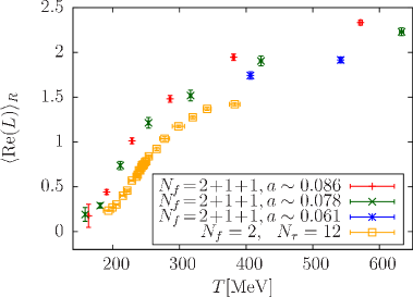
It is shown in the left panel of Fig. 1 and seen to rise monotonously in the crossover region. For comparison we show in the same figure also our two-flavor data obtained at the same value of the pion mass. For large temperatures ($\geq 350\mathrm{~{}MeV}$) a remaining cutoff effect is visible by a tendency of the data to attain lower values with decreasing lattice spacing. However, around the inflection point and thus in the vicinity of the crossover, the data from our two coarsest lattice spacings agree with each other. Thus we conclude that for $N_{\tau}\geq 8$ cutoff effects are small. From the overall view we note that with inclusion of the dynamical second quark generation the curve is shifted towards smaller temperatures as compared to $N_{f}=2$.

Figure 1: Left: The renormalized Polyakov loop. The transition region is so far only covered entirely by the two sets with coarsest lattice spacings. Right: The renormalized light chiral condensate according to Eq. (5).

The chiral condensate $\langle\bar{\psi}\psi\rangle$ is evaluated by means of the technique of noisy estimators using quark matrix inversions on 24 Gaussian noise vectors. These as well as all $T=0$ fermion matrix inversions were calculated on local GPU clusters. Its additive quadratic, mass dependent divergence ($\propto\frac{\mu}{a^{2}}$) can be removed by subtracting the corresponding condensate at the same mass for $T=0$ [3]:

$$R_{\langle\bar{\psi}\psi\rangle}=\frac{\langle\bar{\psi}\psi\rangle^{T,\mu}_{l}-\langle\bar{\psi}\psi\rangle^{T=0,\mu}_{l}+\langle\bar{\psi}\psi\rangle^{T=0,\mu=0}_{l}}{\langle\bar{\psi}\psi\rangle^{T=0,\mu=0}_{l}}\,.$$ (5)

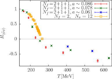
The multiplicative renormalization factor in the denominator is obtained by extrapolating the zero temperature condensate to the chiral limit. To this end we have used a linear ansatz in the light mass, which was sufficient and has yielded acceptable fits. For the coarsest lattice spacing the pion mass had to be restricted to values lower than 370 MeV to obtain an acceptable fit. We added a trivial unity in Eq. (5) in order to account for the presence of symmetry breaking in the hadronic phase. The same procedure has been followed in the two-flavor case for which we show $R_{\langle\bar{\psi}\psi\rangle}$ for comparison in the right panel of Fig. 1. Similarly to the Polyakov loop we observe stronger lattice artefacts in our data above $T=350\mathrm{~{}MeV}$. Whether these alone can be blamed for the drop of $R_{\langle\bar{\psi}\psi\rangle}$ below zero above the transition (where it is expected to vanish) should be further studied when more data for our finest lattice spacing becomes available also at lower temperature. Note again that around the crossover lattice spacing artefacts seem to be small and that the $N_{f}=2+1+1$ curve is shifted towards lower values of the temperature as was observed for the renormalized Polyakov loop, too.

4 Pseudo-Critical Temperature

Having now the strange quark at our disposal, another prescription using a suitable subtraction of the strange quark condensate involving the light and strange masses can be used to eliminate the divergence in the light condensate. This procedure is used in the literature [8]:

$$\Delta_{l,s}=\frac{\langle\bar{\psi}\psi\rangle_{l}-\frac{\mu_{l}}{\mu_{s}}\langle\bar{\psi}\psi\rangle_{s}}{\langle\bar{\psi}\psi\rangle^{T=0}_{l}-\frac{\mu_{l}}{\mu_{s}}\langle\bar{\psi}\psi\rangle^{T=0}_{s}}\,.$$ (6)

Figure 2: Left: The light chiral condensate according to Eq. (6). Right: The disconnected part of the light chiral susceptibility with a polynomial fit to estimate the pseudo-critical temperature. The previously obtained $N_{f}=2$ data is included for comparison. The vertical bars indicate the estimated pseudo-critical temperatures.

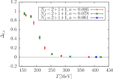
The strange quark condensate is obtained in the Osterwalder-Seiler setup [9, 10], and the bare strange mass has been set as to reproduce the physical $\bar{s}\gamma_{\mu}s$-mass. As opposed to $\langle\bar{\psi}\psi\rangle_{R}$ of Eq. (5), the thus subtracted condensate shows no lattice spacing artefacts over the whole studied range of temperatures and shows a smooth order parameter-like behavior.

In order to estimate the crossover temperature we have evaluated the disconnected part of the chiral susceptibility

$$\sigma^{2}_{\bar{\psi}\psi}=V/T\left(\left<(\bar{\psi}\psi)^{2}\right>-\left<\bar{\psi}\psi\right>^{2}\right)\;.$$ (7)

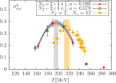
Similar to the two-flavor case this quantity shows a maximum at the crossover temperature as can be appreciated in the right panel of Fig. 2. The data of our two coarsest lattice spacings have been fitted with a polynomial ansatz in the temperature range $160\leq T\leq 240\mathrm{~{}MeV}$ and gives a value of $T_{\chi}=197.4(1.6)$. The corresponding fit curve is included in the figure. From varying the lower and upper bounds of fitting we estimate an additional systematic error ($\sim 3\mathrm{~{}MeV}$) which we add in quadrature. For comparison we show the corresponding $N_{f}=2$ data, which is located at larger temperatures consistent with the observations from the other observables. The result for $T_{\chi}$ is summarized in the following table:

	$N_{f}=2+1+1$	$N_{f}=2$
$T_{\chi}$ [MeV]	$197(4)$	$217(5)$

.

5 The Trace Anomaly

The standard approach that is taken in lattice calculations to evaluate the EoS as the temperature dependence of pressure $p(T)$ and energy density $\epsilon(T)$ begins with evaluating the trace anomaly

$$I=\epsilon-3p=-\frac{T}{V}\frac{d\ln Z}{d\ln a}\;.$$ (8)

As $I/T^{4}$ is identical to a derivative of the reduced pressure $p/T^{4}$ with respect to the $\log$ of temperature

$$\frac{I}{T^{4}}=T\frac{\partial}{\partial T}\left(\frac{p}{T^{4}}\right)\;,$$ (9)

the pressure itself may be evaluated as an integral once $I(T)$ is known. The trace anomaly Eq. (8) which constitutes a total derivative of the partition function with respect to the lattice spacing is calculable on the lattice by taking the derivative of the lattice action with respect to the bare parameters first. The terms corresponding to the derivatives of various parts of the action have to be rendered finite by subtracting the corresponding expectation value at $T=0$. We denote the result by $\left<\ldots\right>_{\mathrm{sub}}$ in the following. The lattice spacing dependence is encoded in the $\beta$-function as well as in additional functions encoding the running of the masses. In what follows we restrict ourselves to the gauge parts of the trace anomaly which are most easily evaluated and make up its dominant part:

$$I_{g}=\frac{\epsilon-3p}{T^{4}}(\mathrm{gauge~{}part})=a\frac{d\beta}{da}\left<S_{g}\right>_{\mathrm{sub}}\,.$$ (10)

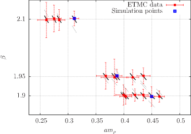
In order to evaluate the $\beta$-function $a\frac{d\beta}{da}$ we adopt a similar strategy as in Ref. [4] and perform a global fit of the coupling in terms of the rho meson mass ($m_{\rho}$) and the charged pion mass ($m_{\pi}$):

$$\beta=c_{0}\log{\left(c_{1}\left(am_{\rho}\right)\right)}+c_{2}\left(am_{\rho}\right)^{2}+c_{3}\frac{\left(am_{\rho}\right)}{\left(am_{\pi}\right)}$$ (11)

For the determination of the rho mass we have used propagators that have been calculated for [11]. We propagate the errors on the hadron masses to errors on the bare couplings $\beta$ by standard error propagation neglecting correlations and evaluate the value of $\chi^{2}$ per degree of freedom from these. We obtain a satisfying fit with $\chi^{2}/\mathrm{dof}\approx 1.0$ that is shown in the left panel of Fig. 3. The $\beta$-function is then evaluated using the rho mass to set the scale as

$$a\frac{d\beta}{da}=(am_{\rho})\frac{d\beta}{d(am_{\rho})}$$ (12)

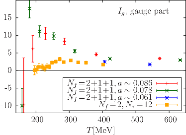
at the chosen simulation points (depicted in blue in the left panel of Fig. 3). We show additionally the slopes $\frac{d\beta}{d(am_{\rho})}$ at all zero-temperature ETMC data points as thick black arrows. Thin grey arrows indicate the $\beta$-values the fit chooses for the different points. In order to estimate the uncertainty connected with the choice of the fit function we have varied it by adding a term $\propto\left(am_{\rho}\right)^{2}/\left(am_{\pi}\right)^{2}$ or by replacing the term $\propto\left(am_{\rho}\right)^{2}$ with it. The maximal magnitude of change in the $\beta$-function was then taken as a systematic error and included additionally to the statistical error of $I_{g}$. In the right panel of Fig. 3 the gauge part of the trace anomaly is shown together with the preliminary two-flavor result from Ref. [12]. As compared to the two-flavor case the peak in $I_{g}/T^{4}$ evaluated for $N_{f}=2+1+1$ is significantly higher as well as shifted to smaller temperatures.

Figure 3: Left: Fit of the $\beta$-function (Eq. (11)). Right: Gauge part of the trace anomaly $I_{g}$ defined in Eq. (10). For comparison we again show the corresponding quantity in the two flavor case.

6 Conclusions and Outlook

We have presented first results of a fixed-scale finite-temperature study of the QCD crossover with a full dynamical second quark generation in the Wilson twisted mass lattice regularization. As a first step we have concentrated on a single pion mass value together with three lattice spacings in order to estimate cutoff effects. We find the latter to be small around the transition region for several observables, while at large temperatures they are significant. From the maximum in the disconnected part of the bare chiral susceptibility we have estimated the temperature of the chiral crossover. Comparing to the two-flavor case previously studied, we observe a downward shift of the transition temperature by approximately $20$ MeV. All studied observables show this behavior.

Furthermore, we have presented results for the gauge part of the trace anomaly. We are currently working on the inclusion of the various fermionic contributions and on the determination of the remaining mass related $\beta$-functions. As the chosen fixed-scale approach can only provide a limited resolution in temperature, even more so if only even values of $N_{\tau}$ are considered, we are working on including also odd numbers of temporal lattice sites. Furthermore, we will address lower quark masses in the near future.

References

- [1] MILC Collaboration, A. Bazavov et al., “Towards a QCD equation of state with 2 + 1 + 1 flavors using the HISQ action,” PoS LATTICE2012 (2012) 071.
- [2] C. Ratti et al., “Lattice QCD thermodynamics in the presence of the charm quark,” Nucl.Phys. A904-905 (2013) 869c–872c.
- [3] tmfT Collaboration, F. Burger et al., “The thermal QCD transition with two flavours of twisted mass fermions,” Phys. Rev. D 87 (2013) 074508.
- [4] WHOT-QCD Collaboration, T. Umeda et al., “Equation of state in 2+1 flavor QCD with improved Wilson quarks by the fixed scale approach,” Phys.Rev. D85 (2012) 094508.
- [5] ETM Collaboration, R. Baron et al., “First results of ETMC simulations with N(f) = 2+1+1 maximally twisted mass fermions,” PoS LATTICE2009 (2009) 104, arXiv:0911.5244 [hep-lat].
- [6] ETM Collaboration, R. Baron et al., “Light hadrons from Nf=2+1+1 dynamical twisted mass fermions,” PoS LATTICE2010 (2010) 123, arXiv:1101.0518 [hep-lat].
-
[7]
K. Jansen and C. Urbach, “tmLQCD: A Program suite to simulate Wilson Twisted
mass Lattice QCD,” Comput.Phys.Commun. 180 (2009) 2717–2738
A. Abdel-Rehim et al., “Recent developments in the tmLQCD software suite,” PoS LATTICE2013 (2013) 414 - [8] M. Cheng et al., “The QCD equation of state with almost physical quark masses,” Phys.Rev. D77 (2008) 014511.
- [9] K. Osterwalder and E. Seiler, “Gauge Field Theories on the Lattice,” Annals Phys. 110 (1978) 440.
- [10] R. Frezzotti and G. Rossi, “Chirally improving Wilson fermions. II. Four-quark operators,” JHEP 0410 (2004) 070.
- [11] F. Burger et al., “Four-Flavour Leading Hadronic Contribution To The Muon Anomalous Magnetic Moment,” arXiv:1308.4327 [hep-lat].
- [12] tmfT Collaboration, F. Burger et al., “Pseudo-Critical Temperature and Thermal Equation of State from Twisted Mass Lattice QCD,” PoS LATTICE2012 (2012) 068, arXiv:1212.0982 [hep-lat].