Trade-offs Computing Minimum Hub Cover toward Optimized Graph Query Processing

Abstract

As techniques for graph query processing mature, the need for optimization is increasingly becoming an imperative. Indices are one of the key ingredients toward efficient query processing strategies via cost-based optimization. Due to the apparent absence of a common representation model, it is difficult to make a focused effort toward developing access structures, metrics to evaluate query costs, and choose alternatives. In this context, recent interests in covering-based graph matching appears to be a promising direction of research. In this paper, our goal is to formally introduce a new graph representation model, called Minimum Hub Cover, and demonstrate that this representation offers interesting strategic advantages, facilitates construction of candidate graphs from graph fragments, and helps leverage indices in novel ways for query optimization. However, similar to other covering problems, minimum hub cover is NP-hard, and thus is a natural candidate for optimization. We claim that computing the minimum hub cover leads to substantial cost reduction for graph query processing. We present a computational characterization of minimum hub cover based on integer programming to substantiate our claim and investigate its computational cost on various graph types.

I Introduction

Queries over graph databases can be classified broadly into whole graph at-a-time, and node at-a-time processing, and framed as a subgraph isomorph computation problem (e.g., [1, 2]) under a set of label mapping constraints, generally known as graph matching. Techniques such as GraphQL [3], QuickSI [4] and earlier research such as VFLib [5] and Ullmann [6] fall in the former category while TALE [7], and SAPPER [8] are representative of the latter. The advantage of the node at-a-time graph processing approach is its inherent ability to prune search space based on target node matching conditions. Node indices are the most common pruning aid used in most of these processing methods although indices on paths [9], frequent structures [10], node distances [1, 10, 11], etc. have also been used. The key difference is in the ways indices are exploited for the construction of the target database graphs from their parts (i.e., the edges).

The effectiveness of the node at-a-time methods, however, largely depends on the query type such as subgraph isomorphism, approximate matching, path queries and so on, as well as on the index structure used. In other words, universal indexing methods are not always suitable for all queries, and therefore specialized indices are often constructed to process a query (e.g., GraphGrep [9], TALE, and SAPPER) and never maintained. Thus, it is not apparent if the index structure is switched, how an algorithm will perform leaving an open question if generic index structures can be leveraged in a way similar to relational query processing with popular indices such as B+ trees, extendible hashing and inverted files.

In order to decouple the index selection from the query expressions, and to subsequently use indices as a strategic instrument to compute alternative query plans, we focus on a representation method for graphs that is independent of the underlying access structures. Our goal is to propose the “hub” as the unit of graph representation that tells us all we need to know about a node or vertex of a graph. Intuitively, each node in a graph as hub “covers” all the edges involving its neighbors and itself. For example, the hub $u_{5}$ in figure 1(a) covers the edges $(u_{1},u_{5}),(u_{1},u_{2}),(u_{2},u_{5}),(u_{2},u_{3}),(u_{3},u_{5})$ and $(u_{5},u_{6})$ as a unit structure (shown as the purple edges).

Figure 1: Example: Query graphs $q_{1}$ and $q_{2}$, and data graph $d$.

The concept of hub we have in mind can be thought of as a convenient extension of Ullmann’s adjacency matrix [6] and feature structure indexing [12, 13] in that we localize the adjacency matrix at the node level and consider only a single feature, edges among the neighbors. Consequently only structures that are part of a hub are stars (neighbors with no shared edge with other neighbors) and triangles (neighbors sharing edge with other neighbors). In figure 1(a), vertex $u_{5}$ has two triangles $\triangle u_{1}u_{2}u_{5}$ and $\triangle u_{2}u_{3}u_{5}$, and a star $(u_{5},u_{6})$ (in this case just an edge). Whereas vertices $v_{9}$ and $v_{11}$ in figure 1(b) have a star (with two edges $(v_{8},v_{9})$ and $(v_{9},v_{10})$ with $v_{9}$ as their center), and three triangles ($\triangle v_{4}v_{7}v_{11}$, $\triangle v_{8}v_{7}v_{11}$, and $\triangle v_{4}v_{8}v_{11}$) respectively.

Our goal is to use these atomic structural cues to match shapes for the purpose of graph matching. For example, to match the query graph $q_{1}$ in figure 1(a) with the data graph $d$ in figure 1(b), we look for individual node structures that are identically connected and depending on the matching requirement, have identical labels. The next step is to piece together these individual matches to see if the composed structure is the target graph. The cost of this search usually is dominated by the cost of piecing together the components and testing if the process is yielding the target graph.

In this example, we can contemplate several different types of graph matching that can be conceived as the variants of subgraph isomorphism though in the literature, only the structural isomorphs and match isomorphs defined below are prevalent. We therefore will consider only these two types of matching in the remainder of this paper.

• structural subgraph isomorph, where only the node IDs (not the labels) are mapped from query graphs to data graphs using and injective function.

• label subgraph isomorph, on the other hand, requires an injective mapping of both node IDs and node labels from query graph to data graph.

• full subgraph isomorph extends label subgraph isomorphic matching to include edge labels in the mapping.

• match subgraph isomorph uses an equality function on the definition of full subgraph isomorph to achieve exact matching of node and edge labels while maps node IDs using an injective function.

Among the above four modes of matching, structural subgraph isomorphism is the least restrictive or selective, and so most computationally expensive. While the match subgraph isomorphic matching (in the literature it is known as labeled graph matching) is the most restrcitive/selective, full and and label subgraph isomorphism are increasingly less so. The idea here is that by combining different selection and mapping constraints, called matching mode, we can capture most popular graph matching concepts and go beyond current definitions. Traditional deep equality $\stackrel{{\scriptstyle d}}{{=}}$ operator [14] in object-oriented databases can be used to test if two graphs (or a subgraph) are equal (or contained in the other graph) by requiring that node IDs and labels be identical. Finally, by requiring that the two graphs have equal number of nodes, we can also achieve graph isomorphism for each case above.

I-A Main Motivation

The vertex labeled graphs in figure 1 show two query graphs $q_{1}$ and $q_{2}$, and a data graph $d$ respectively. In these graphs, each node has a unique node ID such as $u_{i}$, $v_{j}$ and $w_{k}$, and a label such as $A$, $B$ and $C$ (shown in uppercase with unique color codes). If all the labels are empty, the graph is considered unlabeled. If we matched query graph $q_{1}$ with the data graph $d$ for structural subgraph isomorphism, we will compute the green, brown and red matches, among others, as we are only required to map node IDs. However, if we were to compute match subgraph isomorphs, only solution we can compute then is the green subgraph. If label subgraph isomorphs were being sought instead, the solution will include the brown subgraph where we map pink (C) to pink, green (D) to blue (A), mustard (B) to mustard, and blue to green, along with the obvious green subgraph. Let us illustrate this naive matching process using figures 1 and 2.

Figure 2: Candidate generation for query graph hub $u_{2}$ on data graph $d$.

Since there are six nodes in the graph $q_{1}$, a total of six hubs are possible. Similarly, the graph $d$ can be represented by a total of eleven hubs. Let us first match $q_{1}$ with $d$ in match subgraph isomorphism mode. Under this constraint, for hub $u_{5}$ (shown clock-wise rotated by $180^{\circ}{\rm C}$ in purple in figure 2(a)), we can only find one hub, hub $v_{2}$ shown in figure 2(b), in $d$ which is a supergraph of hub $u_{5}$ and can produce a structure identical to $u_{5}$ (shown as red edges) on proper mapping of the node IDs. These structures are called candidate graphlets. However, if we choose to match in structural or label subgraph isomorphism mode, we can find more hubs as capable of generating candidates structures. For example, in label subgraph isomorphism mode, hubs $v_{4}$ and $v_{5}$ can also generate candidates (possible candidate structures are shown in red, purple and green) as shown in figures 2(c) and 2(d).

To complete the matching, we can continue to match all the other hubs in $q_{1}$ in a similar way, and by applying the substitutions generated for each set of previous matches to the candidate hubs to eventually compute the green match as shown in figure 1(b). These graphlets can be joined or pieced together in both bottom-up fashion using a process similar to natural join, or in top-down manner using a depth-first search. In both cases, the graphlets that do not stitch to form the target graph will eventually be eliminated.

Clearly, the dominant cost in this naive algorithm is in candidate generation. Therefore, it would be prudent to seek opportunities to curtail the candidates that do not have a realistic chance of contributing to the result, or will produce redundant candidates. For example, we can be smarter and choose to match $u_{4}$ or $u_{5}$ only without compromising the outcome. We can further speed up the process by noticing that $u_{4}$ is a green D node and there are four such nodes in $d$, all of which will generate a total of twelve candidates even though only four will survive the node mapping, and only one will join with the first candidate to complete the computation. On the other hand, if we decided to use $u_{3}$, we will generate six candidates ($v_{3}$ is not one of them) of which only one will survive the mapping and eventually the response. Furthermore, if we started initially with $u_{4}$, and then try to map $u_{5}$, the number of candidates generated will be even higher although the response computed will still be the same. Interestingly though, if the query is $q_{2}$ (note the similarity of the two queries except that $w_{4}$ is now purple), it is definitely better to start matching with $w_{4}$, because there is only one candidate and it will fail to produce the response in the next step, as expected.

These observations lead us to devise the following query processing strategy. First, we reduce the number of hubs or graphlets in the query graph that we must match based on a new notion of edge covering in graph theory, called the minimum hub cover (MHC). A minimum hub cover essentially means a subset of the nodes in a graph accounts for all the edges in a graph. Secondly, the concept of MHC helps exploit available meta-data on nodes to order the nodes in priority order based on their selectivity to prune search space, that we call a query plan. In ordering the nodes, we explore the nodes that will most likely produce the least number of candidates first. Given the fact that a query graph may have multiple MHCs, it also offers us the opportunity to choose the best query plan for a database instance. Finally, we are now able to use access structures such as hash index and set index to find only the nodes that are relevant for expanding nodes at a given point in a query plan. In fact, the matching algorithm 2 uses two such indices $I_{H}$ and $I_{S}$. The query plan can be implemented as a top-down or bottom-up procedure based on the expected number of candidates and a choice can be made based on the expected cost. In particular, it is also possible to reorder the query plan in a top-down procedure to prune search space dynamically in a way similar to best-first search.

I-B Organization of the Paper

Covering based graph matching is proving to be an interesting and emerging research direction although we are aware of only Sigma [15] which used set covering directly for matching very small graphs, while [16, 17] indirectly used covering for graph matching tangentially. Our goal in this paper, however, is to formally introduce the idea of graph representation using graphlets and graph query processing using the minimum hub cover of query graph graphlets. Our focus is to convince the skeptics that these two concepts help achieve the separation in graph representation and storage, indexing, query plan generation, and query optimization conveniently.

Once this model is accepted in principle, two main computational problem emerge both of which are computationally hard – computing MHC and graph matching using subgraph isomorphism as the primary vehicle. In this paper, we only address the first issue, that is the computational aspects of MHC. But for the sake of completeness, we also briefly present an outline of the cost-based optimization strategy for the ordering of graphlets in the MHC as a candidate query plan, and a query processing algorithm that uses indices for the execution of a query plan. By doing so, we demonstrate that cost-based query optimization is feasible if we are able to compute the MHC of a query graph. Finally, we believe that even if algorithms such as SUMMA [19], NOVA [20], TALE, and SAPPER do not use a notion similar to hubs as we do, they do use the notion of neighborhood and will benefit from the development presented in this paper if they consider a similar covering, i.e., edge or vertex covers, of the queries. The results in this paper then becomes directly relevant to those research as well because we show how the cost of covering computation may vary depending on the type and parameters of the graphs being considered.

The remainder of the paper is organized as follows. We discuss background of the research related to MHC in section II. In this section, we also discuss related research in covering computation based on which we formulate our characterization of MHC. The formal treatment of MHC and its application in query plan generation is discussed in section III. Similar to other covering problems such as set cover, and minimum vertex cover, MHC turns out to be an NP-complete problem as well. Therefore, it can be framed as an optimization problem and made a candidate for heuristic solutions. In section III-E, we discuss an integer programming formulation of the MHC problem as a prelude to our main results on its computability. We have implemented the algorithm using the IBM ILOG optimization engine CPLEX. The experimental results in section V based on the design in section IV suggest that solving MHC to optimality is not a concern for many graph types. A summary of interesting and possible future research issues that are still outstanding is discussed in section VI. We finally conclude in section VII.

II Background and Related Research

In our earlier research on IsoSearch [21], we have shown that the notion of structural unification helps to extract all possible matches of two hubs under a mapping function or a substitution list. While this atomic matching process generates a potentially large candidate pool, we were able to avoid the large cost related to testing for conformity of the candidate target structure with that of the query graph that most other algorithms incur. In our case, conformity is an eventuality and automatic if a match exists. We have also shown that IsoSearch performs significantly better than traditional algorithms such as Ullmann and VFLib, have a significantly low memory footprint, and is able to handle arbitrary sized query and data graphs (because we handle only pairs of graphlets at a time). The concepts of hubs and minimum hub covers also help model various definitions of exact graph matching along the lines of [22, 23, 10], as well as approximate graph matching in the spirit of TALE.

Tangentially to this research, in our recent top-$k$ graph matching algorithm TraM [24], we have explored the idea of hub matching as a unit of comparison and computed structural distance of attributed hubs without the need for explicit use of indices. In this approach, we have developed a quantification for a hub’s structural feature as a random walk score [25]. Since random walk scores encompass the global topological properties of a node as a hub, from the standpoint of graph matching, it can be used to compare topological orientation and relative importance of graph nodes. These scores thus effectively capture the topological likeness and structural cues shared among the hubs, and were effectively exploited for approximate graph matching in TraM. A similar method was used in [26] to compute computation of similarities of nodes of a graph for collaborative recommendation. The random walk based approach, however, does not offer much opportunity for cost-based query optimization based on the evolving states of the database extension in ways similar to [27, 28] because it is largely similar in nature to many algorithmic counterparts such as SUMMA, NOVA, TALE, and SAPPER.

As we shall elaborate in the subsequent part of this section, the MHC problem is closely related to two well-known combinatorial optimization problems, the set covering problem (SCP) and the minimum vertex cover (MVC) problem, which are, in turn, share a similar mathematical programming model. We next discuss the relationship between the MHC problem and the MVC problem, and then tie this discussion to a general set covering formulation that we also adopt in this work.

Let us start with the integer programming (IP) model for the MVC problem:

minimize $$\sum_{j\in V}x_{j},$$ (1)

subject to $$x_{i}+x_{j}\geq{1} (i,j)\in E,$$ (2)

$$\ x_{j}\in\{0,1\}, j\in V,$$ (3)

where $x_{j}$ is a binary variable that is equal to 1, if vertex $j$ is in the cover and 0, otherwise. The objective function (1) evaluates the total number of vertices in the cover. Constraints (2) ensure that every edge is covered by at least one vertex, and constraints (3) enforce binary restrictions on the variables. To give a concrete example, suppose that we are trying to find the optimal MVC in the graph shown in figure 1(a). The corresponding IP model is then given by

$$\mbox{minimize}~{}~{}x_{1} {}+ {}x_{2} {}+ {}x_{3} {}+ {}x_{4} {}+ {}x_{5} {}+ {}x_{6}$$ ,

$$\mbox{subject to}~{}~{}x_{1} {}+ {}x_{2} {}\geq{1},\ \ \ [(u_{1},u_{2})]$$

$$x_{1} {}+ {}x_{5} {}\geq{1},\ \ \ [(u_{1},u_{5})]$$

$${}x_{2} {}+ {}x_{3} {}\geq{1},\ \ \ [(u_{2},u_{3})]$$

$${}x_{2} {}+ {}x_{5} {}\geq{1},\ \ \ [(u_{2},u_{5})]$$

$${}x_{3} {}+ {}x_{4} {}\geq{1},\ \ \ [(u_{3},u_{4})]$$

$${}x_{3} {}+ {}x_{5} {}\geq{1},\ \ \ [(u_{3},u_{5})]$$

$${}x_{5} {}+ {}x_{6} {}\geq{1},\ \ \ [(u_{5},u_{6})]$$

$$x_{1} {}x_{2} {}x_{3} {}x_{4} {}x_{5} {}x_{6} {}\in\{0,1\}.$$ , , , , ,

The model minimizes the total number of selected vertices while satisfying the coverage constraints written for each edge. For the sake of clarity, the edge corresponding to a constraint is designated at the end of each line within the brackets. The first constraint, for example, implies that the edge $(u_{1},u_{2})$ can be covered by vertices $u_{1}$ and $u_{2}$. Since an edge can be covered only by the vertices incident to it, each constraint in the IP formulation of the MVC problem involves exactly two variables. In this particular example, $\{u_{2},u_{5}\}$ is the unique optimal solution.

When it comes to the mathematical programming model of the MHC problem, we need to pay attention to the fact that a vertex (as a hub) covers not only the edges incident to itself but also those edges between its immediate neighbors. Using this fact, we obtain the following IP formulation of the MHC problem for the graph in figure 1(a):

$$\mbox{minimize}~{}~{}x_{1} {}+ {}x_{2} {}+ {}x_{3} {}+ {}x_{4} {}+ {}x_{5} {}+ {}x_{6}$$ ,

$$\mbox{subject to}~{}~{}x_{1} {}+ {}x_{2} {}+ {}x_{5} {}\geq{1},$$

$${}x_{2} {}+ {}x_{3} {}+ {}x_{5} {}\geq{1},$$

$${}x_{3} {}+ {}x_{4} {}\geq{1},$$

$${}x_{5} {}+ {}x_{6} {}\geq{1},$$

$$x_{1} {}x_{2} {}x_{3} {}x_{4} {}x_{5} {}x_{6} {}\in\{0,1\}.$$ , , , , ,

Notice that unlike the IP formulation of the MVC problem, the number of constraints reduces since multiple edges can be covered by the same set of vertices. For instance, the second constraint shows that vertices $u_{2}$, $u_{3}$ and $u_{5}$ cover the edges $(u_{2},u_{3}),(u_{2},u_{5})$, and $(u_{3},u_{5})$. As a consequence of this hub property, the number of variables appearing in a constraint is greater than or equal to two. In fact, this number can easily go up to the number of vertices, because the vertices incident to an edge may be connected to all other vertices forming an abundant number of triangles. Clearly, the cardinality of the MHC can be far less than that of the cardinality of the MVC due to the additional non-incident edges covered by those vertices in a triangle. Therefore, for triangle-free graphs, the optimal solutions for the MHC problem and the MVC problem naturally coincide.

II-A Minimum Hub Cover: As a Special Case of Set Covering

The above formulations of the MVC and MHC problems actually show that both problems are just the special cases of the SCP. Given a fixed number of items and a family of sets collectively including (covering) all these items, the objective of the SCP is to select the least number of sets (minimum cardinality collection) such that each item is in at least one of these selected sets. If an edge corresponds to an item and a set is formed with the edges that can be covered by each vertex, then the connection between the SCP and the MHC problem as well as the MVC problem can easily be established. To formalize this discussion, below we give the generic IP formulation for the MHC problem:

minimize $$\sum_{j\in V}x_{j},$$ (4)

subject to $$x_{i}+x_{j}+\sum_{\begin{subarray}{c}(i,k)\in E\\ (j,k)\in E\end{subarray}}x_{k}\geq{1}, (i,j)\in E,$$ (5)

$$\ x_{j}\in\{0,1\}, j\in V.$$ (6)

Again, the binary variable $x_{j}$ is equal to 1, if vertex $j$ is in the hub cover, and the objective is to minimize the number of vertices used in the cover. Constraints (5) ensure that every edge is covered by at least one hub node in the cover. Finally, the constraints (6) enforce the binary restrictions on the variables. Although the number of constraints seems equal to the number of edges, we remind that multiple edges can be covered by the same set of vertices (see MHC example above).

The introduction of the hub cover concept to the literature is quite recent [18]. Thus, to the best of our knowledge, the solution methods for the MHC problem have not been examined in the literature. However, closely related problems, the MVC problem and the SCP, have been extensively studied before. Take the MVC problem; approximation algorithms [29, 30], heuristic solutions [31], evolutionary algorithms [32, 33] can be listed among those numerous solution methods. The SCP is no different. From approximation algorithms [34, 29] that have good empirical performances to randomized greedy algorithms [35, 36], and from local search heuristics [37, 38] to different meta-heuristics [39, 40, 41] have been proposed for solving the SCP.

III Minimum Hub Cover: The Formal Model

As mentioned earlier, in graph $q_{1}$, node or hub $u_{5}$ covers the edges $(u_{1},u_{5})$, $(u_{1},u_{2})$, $(u_{2},u_{5})$, $(u_{2},u_{3})$, $(u_{3},u_{5})$ and $(u_{5},u_{6})$. Similarly, the hub $u_{3}$ covers edges $(u_{3},u_{2})$, $(u_{5},u_{2})$, $(u_{3},u_{5})$ and $(u_{3},u_{4})$. Since the set of hubs $\{u_{5},u_{3}\}$ covers all the edges of $q_{1}$, this set is called a hub cover of $q_{1}$, denoted $cover(q_{1})$, and so are the sets $\{u_{5},u_{4}\}$, $\{u_{2},u_{6},u_{4}\}$, and $\{u_{1},u_{5},u_{4}\}$. However, for the purposes of graph matching, it is sufficient if we matched the set $\{u_{5},u_{3}\}$ with another graph as any super set this will not add any more new node or edge matching. We thus call this set the minimum hub cover of $q_{1}$, denoted $MHC(q_{1})$ and formalized in the following definition.

Definition III.1 (Minimum Hub Cover)

For a given graph $G=<V,E>$, $M\subseteq V$ is a minimum hub cover of $G$, denoted $MHC(G)$, if $M$ is the smallest set, and for every edge $<s,d>\in E$, either $d\in M$ or $s\in M$, or there exists edges $<s,c>\in E$ and $<d,c>\in E$, and $c\in M$. The set of all $MHC(G)$ is denoted as $\Gamma(G)$.

It should be apparent that given a graph $G=\langle V,E\rangle$, the number of hub nodes in $M$ lies within the range $1\leq|M|\leq\frac{|V|}{2}$. For example, both $\{u_{5},u_{3}\}$ and $\{u_{5},u_{4}\}$ are in $\Gamma(q_{1})$, and $|\{u_{5},u_{3}\}|=|\{u_{5},u_{4}\}|$. It should also be apparent that hubs in a given MHC ensures edge connectivity because all edges are covered. But it is likely that a given sequence of hubs may not retain edge connectivity, and thus ordering of the elements in $MHC(G)$ matters and as such this ordering relationship is a key to processing queries efficiently. Intuitively, the query optimization approach we present essentially is the problem of computing the set $\Gamma(Q)$ when computable, then ordering the elements in each set $c_{i}\in\Gamma(G)$ using a cost function $\chi$ (discussed in detail in section III-B) such that $\chi(c_{i})$ is minimized, and then choose MHC $c_{j}$ such that $\chi(c_{j})$ is the minimum among all MHCs in $\Gamma(Q)$ under $\chi$. The least cost ordering relationship implied by $\chi(c_{j})$ is then taken as the query plan to be executed using a depth-first matching algorithm.

III-A Hubs as Graph Representation

Traditionally, graphs are represented as a pair $\langle V,E\rangle$ where $V$ is a set of vertices and $E$ is a set of edges over $V$. Such a representation does not carry any structural information of which vertices are a part of, and they are not visible until structures are constructed from the set of edges. To ease computational hurdles and aid analysis, some models have used vertices and their neighbors as a unit of representation [7], i.e., $r_{v}=\langle v,N\rangle$ where $v$ is vertex in $V$, and $N$ is a set of neighbors such that $(v,n)\in E\Rightarrow n\in N$. A graph is then modeled as a set of such units. While this representation captures some structural cues, it still is pretty basic.

The decision on the degree of structural information that can be captured and exploited is very hard. In one extreme, we have the traditional representation $\langle V,E\rangle$ with no structural information other than the edges, and the GraphQL model where pretty much the entire graph structure is represented as a single XML document. While GraphQL offers most selectivity due to its representation, taking advantage of this in cost-based query optimization is extremely difficult because meta-data now has to be at the largest structural level. The models that are in between are the star structures [7] and dynamically mined frequent feature structures [42, 43] which we believe can generally be difficult to index and maintained with the evolution of the database.

We believe representing a graph as a set of hubs is a prudent compromise because it assures a deterministic model, and yet offers a realistic chance of efficient storage and processing of graph queries. It is deterministic because each hub can be represented as a triple of the form $r_{v}=\langle v,N_{v},B_{v}\rangle$, called a graphlet, where $v\in V$ is a node in graph $G=\langle V,E\rangle$, and $N_{v}\subseteq V$, and $B_{v}\subseteq E$ such that for each $v\in V$ all $n\in N_{v}$ are its immediate neighbors, and every edge $b\in B_{v}$ are edges involving neighbors in $N_{v}$. For unlabeled and undirected graphs, this representation model is sufficient. But for labeled and directed graphs, this simple model can be extended without any structural overhaul. We can now simply define a graph as a set of graphlets, i.e., $G=\bigcup_{\forall v,v\in V}r_{v}$. In fact, in NyQL, we have shown that such a representation can be conveniently captured using traditional storage structures such as nested relations or XML documents.

III-B Cost Function $\chi$ and Graphlet Ordering Relation $\prec$

Given two graphlets $r_{v}$ and $r_{u}$, and a graph $D$, we define an ordering relation $r_{v}\preceq r_{u}$, called the selectivity ordering, between them to mean $r_{v}$ precedes $r_{u}$ (or $r_{v}$ costs less than $r_{u}$ in processing time) in two principal ways.

• First, when the selectivity of $r_{v}$, denoted $sel(r_{v},D)$, is higher than $sel(r_{u},D)$. Technically, $sel(x,G)$ means the number of graphlet instances $r_{y}$ in graph $G$ that satisfy the condition $|N_{y}|\geq|N_{x}|$ and $|B_{y}|\geq|B_{x}|$, and selectivity of $r_{v}$ is higher than that of $r_{u}$ in a graph $G$ if $sel(r_{v},D)\leq sel(r_{u},D)$. We call it node selectivity, denoted $\preceq_{v}$.

• Second, when the selectivity of $N_{v}$ and $B_{v}$, called the structural selectivity and denoted $\preceq_{s}$, is higher than the selectivity of $N_{u}$ and $B_{u}$, denoted respectively as $sel(N_{v},B_{v},D)$ and $sel(N_{u},B_{u},D)$, i.e., $sel(N_{v},B_{v},D)\leq sel(N_{u},B_{u},D)$, where $sel(N_{x},B_{x},D)$ is the number of graphlet instances $r_{y}$ in graph $G$ that satisfy the condition $|N_{y}|\geq|N_{x}|$ and $|B_{y}|\geq|B_{x}|$.

• Finally, the neighbor selectivity (denoted $\prec_{n}$) $sel(N_{v},D)\leq sel(N_{u},D)$ holds where $sel(N_{x},D)$ represents the number of graphlet instances $r_{y}$ in graph $G$ that satisfy the condition $|N_{y}|\geq|N_{x}|$.

The query plan as the total ordering $\prec$ then can be induced from the precedence relationship $\preceq$ of graphlets in $G$ using the procedure Graphlet Ordering in algorithm 1. Algorithm 1 is intuitively explained in figure 3 where we show that the dot nodes are identified first followed by the star nodes and ordered in terms of their selectivity. In figure 3(a), the three components of a graphlet are shown in brown, green and yellow, where the neighbors $N_{v}$ are partitioned in to two sets $mapped(N_{v})\subseteq N_{v}[\theta]$ and unmapped subsets (shown in uppercase). Since an instantiated dot node may only fetch a single hub at the most, this ordering is likely to result in a least cost plan.

Input: A graph $G$, a cost estimator $\chi$, a matching mode and data dictionary.

Output: A total ordering $\prec$ on $G$.

1 Set $i=1$.

2 Choose the most selective graphlet as $r_{v_{i}}$ using node selectivity.

3 while not all graphlet in $\prec$ marked dead do

4       foreach unmarked graphlet $r_{v}$ in $\prec$ order do

5            while $\exists r_{x},r_{x}\in G$ not marked dead and $x\in N_{v}$ (i.e., $x$ is an immediate neighbor of $v$) do

6                  for $\forall r_{y},r_{y}\in N_{v}$ do

7                        if $r_{x}\preceq_{v}r_{y}$ or $r_{y}\preceq_{v}r_{x}\wedge r_{x}\preceq_{s}r_{y}$ holds then

8                              Increment $i$.

9                               Let $r_{v_{i+1}}=r_{x}$.

10                               Mark $r_{v_{i+1}}$ as a dot node, i.e., $r_{v_{i+1}}^{\bullet}$.

11                        

12                  

13            

14      foreach unmarked graphlet $r_{v}$ in $\prec$ order do

15            while $\exists r_{x},r_{x}\in G$ not marked dead and $N_{v}\cap N_{x}\not=\emptyset$ (i.e., $x$ is a 2-hop neighbor of $v$ and share the nodes $N_{v}\cap N_{x}$ as neighbors) do

16                  for $\forall r_{y},N_{y}\cap N_{v}\not=\emptyset$ do

17                        if $r_{x}\preceq_{n}r_{y}$ or $r_{y}\preceq_{n}r_{x}\wedge r_{x}\preceq_{s}r_{y}$ holds then

18                              Increment $i$.

19                               Let $r_{v_{i+1}}=r_{x}$.

20                               Mark $r_{v_{i+1}}$ as a star node, i.e., $r_{v_{i+1}}^{\star}$.

21                        

22                  

23            Mark $r_{v}$ dead.

24      

return Order $\prec$.

Algorithm 1 Graphlet Ordering

(a) Expansion of top node.

(b) Dot and star expansion of $Q$.

Figure 3: Ordering $Q$ based on expected cost using selectivity.

III-C Indices for Efficient Access

Let us also assume that we have a hash index $I_{H}$ that given a node ID (i.e., $v\in V$), returns the graphlet corresponding to $v$, i.e., $I_{H}(v)=r_{v}$. Furthermore, we also have another index $I_{S}$ similar to [44] such that it returns a set of graphlets $R$ given a set of nodes $V_{q}$, and an integer $n_{c}$, i.e., $I_{S}(V_{q},n_{c})\subseteq G$, such that for each $r_{v}\in R$, $V_{q}\subseteq N$, and $|N|\geq n_{c}$. In other words, $I_{S}$ returns all graphlets that contain the set of nodes in $V_{q}$ and have a minimum of $|V_{q}|\leq n_{c}$ neighbors.

III-D Outline of a Query Processor

The graph query processor for exact matching is simple. It is composed of a depth-first search algorithm Find Solutions that maps a sequence of graphlets in a query graph presented in $\prec$ order to a set of graphlets of a data graph using a composable term mapping function $\mu$. Algorithm 2 is assumed to have access to a data graph $D$, one of four graph matching modes, and the indices $I_{H}$ and $I_{S}$.

Input: A stack $T$ with query graph $Q$ in $\prec$ order (initially $r_{v_{1}}$ as the top element), and a substitution list $\theta$ (initially empty).

Output: Set $sol$ of all matched subgraphs of $D$.

1 if stack $T$ empty then

2      Include $Q[\theta]$ in $sol$.

3       return.

4Let $r_{v}=pop(T)$.

5 Apply substitution $\theta$ to $r_{v}$, i.e., $r_{v}\leftarrow r_{v}[\theta]$.

6 if $r_{v}$ is not a dot node and a star node (it is the top node in $\prec$ order) then

7      Retrieve all $r_{x}$ from $D$ such that $|N_{x}|\geq|N_{v}$ and $|B_{x}|\geq|B_{v}$.

8      

9else

10       if $r_{v}$ is a dot node then

11            Retrieve $r_{x}\leftarrow I_{H}(v)$ from $D$.

12            

13      else

14             if $r_{v}$ is a star node then

15                  Let $M=mapped(N_{v})$.

16                   Retrieve all $r_{x}\in I_{S}(M,|N_{v}|)$

17            

18      

19foreach $r_{x}$ do

20      if exists one substructure of $r_{x}$ similar to $r_{v}$ then

21             foreach substructure $r_{y}$ of $r_{x}[\theta]$ similar to $r_{v}$ do

22                   Find Solutions($T,\mu(r_{y},r_{v})\bullet\theta$).

23            

24      else

25             return.

26      

return $sol$

Algorithm 2 Find Solutions

III-E Computational Characterization of Minimum Hub Cover

We formally present the computational characterization of MHC in terms of its complexity class, and using the decision version of the MHC problem (MHC-D) show that the MHC problem is indeed difficult and that it is NP-complete.

Theorem III.1

MHC-D is NP-complete.

Proof:

To show that MHC-D is NP-Complete, we answer the following question: given a graph $G(V,E)$ and an integer $k\leq|V|$, does there exist a subset $C\subseteq V$ with $|V|\leq k$ such that for every edge $(s,d)\in E$, $s\in C$ or $d\in C$ or there exists a vertex $c\in C$ such that both $(s,c)\in E$ and $(d,c)\in E$? First, we argue that MHC-D is in NP because for a given yes-instance and $C^{\prime}\subseteq V$ with $|C^{\prime}|\leq k$, we can verify in polynomial time that every edge in $E$ is covered by $C^{\prime}$. We now complete the proof by a reduction from the MVC problem on triangle free graphs [45]. In triangle-free graphs, for all $(s,d)\in E$ there does not exist a vertex $c$ such that $(s,c)\in E$ and $(d,c)\in E$. Thus, either $s$, or $d$ must be in $C^{\prime}$ to cover the edge $(s,d)$. Consequently, the MHC and the MVC of a graph are equivalent in this class of graphs and MVC is NP-complete for this class of graphs [45]. ∎

IV Experimental Design

The NP-completeness of MHC speaks to the hardness of the solvability in general. The optimization strategy and query plan generation presented in section III, however, calls for the computation of all MHCs of a given query $Q$, i.e., $\Gamma(Q)$, which is indeed a hard problem. In this section, our goal is to design a set of experiments using different graph types, size and graph density parameters to study how the solvability and the quality of MHC solutions depend on these parameters. The goal is to experimentally identify problem classes for which available solutions are practical and acceptable, and the classes for which new heuristic solutions are warranted. We therefore employ different algorithms to show the trade-offs between optimality and computation time over different graph types. Although our experiments and analysis involve producing only one optimal solution for a graph, the insights gained can be leveraged to develop new algorithms to compute $\Gamma(Q)$ or to choose other strategies when computing $\Gamma(Q)$ is infeasible.

The optimal linear programming (LP) and IP solutions are obtained by ILOG IBM CPLEX 12.4 on a personal computer with an Intel Core 2 Dual processor and 3.25 GB of RAM. In all problem instances, the upper limit on the computation is set at 3,600 seconds. The batch processing of the instances is carried out through simple C++ scripts. Our data set includes a total of 830 instances. We have 5 different instances for each combination of a graph type, size, and density parameter to be able to draw conclusions.

IV-A Selected Graph Types and Problem Classes

We have chosen to use the benchmark database graph instances in [46] and our own synthetically generated data set for our numerical study. This is a very large database of different graph types and sizes designed specifically to test the sophistication of (sub)graph isomorphism algorithms. Since we are using subgraph isomorphism as a basic vehicle for graph matching, the instances selected are thus representative of the class of queries we are likely to handle when we solve the MHC problem. The descriptions of the graph instances we have chosen from this collection are listed below.

Randomly connected graphs

These graphs have no special structure and the number of vertices range from 20 to 1000 ($|V|$= 20, 60, 100, 200, 600, 1000). The parameter $\eta$ denotes the probability of having an edge between any pair of vertices. Thus, this parameter, in a sense, specifies the sparsity of a graph. In the database, three different values of $\eta$ (0.01, 0.05, and 0.10) are considered. Our data set includes a set of graphs of different sizes for each value of $\eta$.

Bounded valence graphs

The vertices of the graphs in this class have the same degree (fixed valence). The sizes of the instances are similar to those of the problem class (a). We use three different values of valence – 3, 6 and 9 to obtain graphs of different size and valence.

Irregular bounded valence graphs

These graphs are generated by introducing irregularities in the problem class (b). Irregularity comes from randomly deleting edges and adding them elsewhere in the graph. With this modification, the average degree is again bounded but some of the vertices may have higher degrees. The sizes of the instances are similar to those of problem classes (a) and (b).

Regular meshes with 2D, 3D, and 4D

In graphs with 2D, 3D, and 4D meshes, each vertex has connections with 4, 6, and 8 neighbors, and the numbers of vertices range from 16 to 1024, 27 to 1000, and 16 to 1296, respectively. Similar to the problem classes (a), (b), and (c), we have a set of graphs for each combination of size and dimension.

Irregular meshes

As in class (c), irregular meshes are generated by introducing small irregularities to the regular meshes. Irregularity comes from the addition of a certain number of edges to the graph. The number of edges added to the graph is $\rho\times|V|$, where $\rho\in\{0.2,0.4,0.6\}$. The number of vertices is exactly the same as in problem class (d).

Scale-free graphs

This problem class includes the graphs that follow a power-law distribution of the form

$$P(k)\sim ck^{-\alpha},$$

where $P(k)$ is the probability that a randomly selected vertex has exactly $k$ edges, $c$ is the normalization constant, and $2\leq\alpha\leq 3$ is a fixed parameter. We employed the scale-free graph generator of C++ Boost Graph Library. The generator (Power Law Out Degree algorithm) takes three inputs. These are the number or vertices, $\alpha$ and $\beta$. Increasing the value of $\beta$ increases the average degree of vertices. On the other hand, increasing the value of $\alpha$ decreases the probability of observing vertices with high degrees. The sizes of the instances range from 20 to 1000; $|V|\in\{20,60,100,200,600,1000\}$ to be precise. We considered two values for $\alpha\in\{1.5,2.5\}$ and three values of $\beta\in\{100\times|V|,200\times|V|,500\times|V|\}$. Graphs in social networks, protein-protein interaction networks, and computer networks are examples of this class.

IV-B Solution Methods Used

We choose three solution methods to compute MHC – (i) an exact method to solve the problem to optimality, (ii) adapt two approximation algorithms from the vertex cover literature capable of computing feasible solutions fast, and (iii) a mathematical programming-based heuristic originally proposed for solving the SCP.

IV-B1 Exact algorithm

The IP formulation (4)-(6) is solved by an off-the-shelf solver to optimality. Since the MHC problem is shown to be NP-Hard, this approach may have practical value only for small-to-medium-scale graphs. However, it sets a definitive benchmark for comparing the performances of various heuristics.

IV-B2 Approximation and greedy algorithms

We implemented two different approximation algorithms. First algorithm selects the vertex with the highest degree at each iteration. The aim is to cover as many edges as possible. Next, all covered edges as well as the vertices in the cover are removed from the graph. The algorithm ends when there is no uncovered edge in the graph. The algorithm is called the $H(\Delta)$-approximation algorithm (GR1) for the MVC problem. Here, $\Delta$ is the maximum degree in the graph, and $H(\Delta)$ is evaluated by

$$H(\Delta)=1+1/2+\ldots+1/\Delta.$$

The second algorithm (GR2), the 2-approximation algorithm, is an adaptation of [47] originally proposed for computing a near-optimal solution for the MVC problem. Unlike the previous algorithm, it selects an edge arbitrarily, then both vertices incident to that edge are added to the cover.

IV-B3 Mathematical programming-based heuristics

Yelbay et al. [48] propose a heuristic (MBH) that uses the dual information obtained from the LP relaxation of the IP model of SCP. They show the efficacy of the heuristic on a large set of SCP instances. In their work, the dual information is used to identify the most promising columns and then form a restricted problem with those columns. Then, an integer feasible solution is found by one of the two approaches. In the first approach (MBH), the exact IP optimal solution is obtained by solving the restricted problem. In the second approach, a METARAPS [37] local search heuristic (LSLP) is applied over those promising columns. We use both of these approaches.

V Analysis of Experimental Results

We focus on analyzing and understanding the MHC solution methods in section IV-B on the instances in section IV-A in three different axes: (i) optimal solvability of MHC, (ii) quality of the solutions, and (iii) computational cost of optimal solution. These analyses are aimed at understanding which problem classes are inherently more difficult relative to others so that depending on the application and query, a suitable algorithm can be selected to compute MHC. We also discuss the factors that increase the complexity of the problems.

V-A Optimal Solvability of Minimum Hub Covers

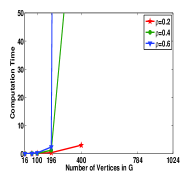
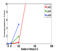
Figure 4 shows how the optimal solution time of CPLEX, an exact method, varies depending on the problem size, class, and structure. The $x$-axis and the $y$-axis represent the number of vertices and the average computation time, respectively. The right-most data point on a line shows the size of the largest instance that can be solved to optimality in a group. In general, its performance is good for small to medium scale graphs. However, in our study, 39 out of 90, 73 out of 285 and 39 out of 180 instances in problem classes (a), (e) and (f), respectively, could not be solved optimally using CPLEX within the time limit. This observation opens the door for heuristics to find acceptable but possibly suboptimal solutions.

(a) Randomly connected graphs

(b) Bounded valence graphs

(c) Irregular bounded valence graphs

(d) Regular meshes with 2D, 3D and 4D

(e) Irregular meshes with 2D

(f) Irregular meshes with 3D

(g) Irregular meshes with 4D

(h) Scale-free graphs with $\alpha=1.5$

(i) Scale-free graphs with $\alpha=2.5$

Figure 4: Average computation time of CPLEX on problem classes as a function of the number of vertices in G and the parameters of the problem classes

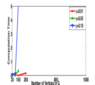
Random graphs

From figure 4(a) we conclude that for randomly connected graphs with more than 200 nodes, optimal solution is not achievable within the bounded time. It also suggests that the density of graphs is a factor that affects the solvability. The solver does increasingly better as the density $\eta$ goes down (up to 0.01) for the same number of vertices. Its sensitivity with respect to the size and density is apparent in the plots for $\eta$ equal to 0.05 and 0.10, i.e., a 16 fold increase in solution time.

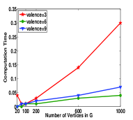
Bounded valance graphs

Compared to random graphs, figure 4(b) shows an improved performance on bounded valence graphs solving all instances under 0.3 seconds. The reason for the performance difference may be due to the considerably higher number of edges in a randomly connected graph (which forces the number constraints in the IP model to go higher) than that of a bounded valence graph. However, although we expect higher solution time for graphs with larger valence, figure 4(b) shows substantially higher time for valence 3 than valences 6 and 9 suggesting other factors may also be playing a role.

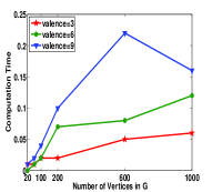
Irregular bounded valance graphs

Although the degree distribution is neither constant nor fully randomly distributed, CPLEX performs similarly to bounded valence graphs. As figure 4(c) shows, all solutions are computed in less than .25 seconds, and that the computation time increases with the increase in valence.

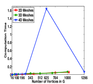
Regular mesh graphs

Figure 4(d) shows that the size of meshes (2D, 3D or 4D) usually does not have any influence on the performance barring the abrupt behavior of the 4D mesh graph. In general, the solution time appears to linearly increase with the increase in graph size, though the increase in time is extremely small.

Irregular mesh graphs

Unlike the irregular bounded valence graphs, mesh graphs are more susceptible to irregularity and the computation time substantially increases with the degree of irregularity. Figures 4(e) through 4(g) show that the sizes of the problems that can be solved to optimality decrease and the computation times increase with increasing degree of irregularity. This result is quite reasonable and expected because increasing irregularity increases the number of edges, and thus the computation time as well. This is also because randomly adding edges to a mesh graph makes it structurally more similar to random graphs, which, as discussed earlier, is inherently hard to solve.

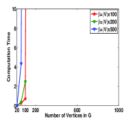
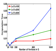
Scale-free graphs

We consider the effect of the two parameters $\alpha$ and $\beta$ on the solvability of the problems. On one hand, increasing $\alpha$ makes the degree distribution sharper, i.e, we observe smaller number of vertices with high degrees. On the other hand, increasing the value of $\beta$ increases the degrees of non-hub nodes. Figures 4(h) and 4(i) represent the optimal solution times of scale-free instances. It is clear that the difficulty of the problem is closely related to parameters $\alpha$ and $\beta$. The figures show that computation times decrease significantly with increasing values of $\alpha$. When $\alpha=1.5$, the instances with more than 100 vertices cannot be solved to optimality within the time limit. When $\alpha=2.5$, however, all of the instances can be solved optimally in less than 0.06 seconds. These figures also show that the computation time increases with increasing values of $\beta$. This means that increasing degrees of non-hub nodes makes the problem more difficult.

V-B Performance Profile of Solution Methods

To study the quality of solutions generated by other solution methods with respect to the optimal solutions computed using CPLEX, we refer to figures 5(a) through 5(e). These plots are called performance profiles of algorithms that depict the fraction of problems for which the algorithm is within a factor of the best solution [49]. Thus, they compare the performance of an algorithm $s$ on an instance $p$ with the best performance observed by any other algorithm on the same instance. The x-axis represents the performance ratio given by

$$r_{p,s}=\frac{\alpha_{p,s}}{\min\{\alpha_{p,s}:s\in S\}},$$

where $\alpha_{p,s}$ is the number of hub nodes in the hub cover when the instance $p$ is solved by algorithm $s$ and $S$ is the set of all benchmark algorithms. The y-axis shows the percentage of the instances that gives a solution that is less than or equal to $\tau$ times the best solution. Recall that CPLEX cannot solve all of the instances in problem classes (a), (e) and (f) to optimality. However, the solver is able to find feasible solutions for some of those unsolved instances (11 out of 39, 44 out of 73, and 24 out of 39 in (a), (e), and (f) respectively). Figure 5 includes all instances except those for which CPLEX cannot find either feasible or optimal solutions within the time limit.

(a) Randomly connected graphs

(b) Bounded valence graphs

(c) Irregular bounded valence graphs

(d) Regular meshes with 2D, 3D and 4D

(e) Irregular meshes

(f) Scale-free graphs

Figure 5: Performance profiles for the algorithms on the problem classes in terms of solution quality

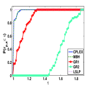
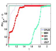
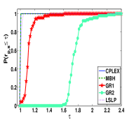
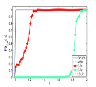
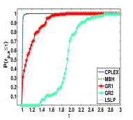
We first analyze how much we sacrifice from the optimality by employing mathematical programming-based heuristics MBH and LSLP. Recall that MBH and LSLP solve the same restricted problem. While MBH tries to solve the problem to optimality, the latter visits alternate solutions in the feasible region. Figure 5(a) shows that 12% of the instances in class (a) where both MBH and LSLP find better feasible solutions than that of CPLEX. Note that, this can happen if and only if CPLEX returns a feasible solution rather than an optimal solution within the time limit. For other problem classes, the performances of the CPLEX and MBH are quite similar. Moreover, these figures show that LSLP is outperformed by MBH and CPLEX on almost 40% and 30% of instances in problem classes (b) and (c) respectively. For the remaining problem classes, the performance of LSLP is also comparable to MBH and CPLEX.

The greedy algorithms return feasible but sub-optimal solutions quickly. Except the scale-free networks, the performances of the greedy algorithms do not change with respect to problem classes. GR2 is known as 2-approximation algorithm for MVC. Figures 5(c) and 5(f) show that there are some instances for which performance ratios of GR2 are higher than 2. Obviously, the approximation ratio of GR1 for MHC problem is higher than 2. Intuitively, the performance of GR1 is supposed to be better when the degree distribution of the vertices is not uniform. Since the average degrees of the vertices are identical or are quite similar for the instances in problem classes (a)-(e), the performance of GR1 does not vary for these problem classes. However, figure 5(f) shows that GR1 finds the optimal or the best solution in 30% of the scale-free instances. This means that the performance of the GR1 is better for the graphs that follow the power-law distribution.

V-C Cost Profile of Solution Methods

The previous two analyses focused on the optimal solvability and the quality of the solutions. In this section we turn our attention to the cost of computing a feasible or optimal MHC solutions in terms of time. Figures 6(a) through 6(f) summarize the distribution of the average computation times of the algorithms over the problem classes. In these plots, the instances for which feasible solutions were not found by any of the algorithm within a time limit are excluded. Each bar in the figure represents the percentage of the instances that are solved within the time interval stated in the legend, e.g., the blue bar for 0.0 to 0.05 seconds. Since LSLP is a local search algorithm, we show both the total computation time and the first time when the best solution is found.

(a) Randomly connected graphs

(b) Bounded valence graphs

(c) Irregular bounded valence graphs

(d) Regular meshes with 2D, 3D and 4D

(e) Irregular meshes

(f) Scale-free graphs

Figure 6: Computation time distributions of the solution methods on the problem classes

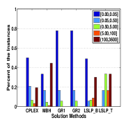
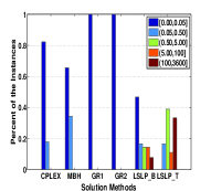
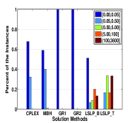
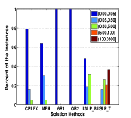
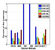
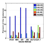
The results clearly show that the solution times of greedy algorithms (GR1, GR2) are much shorter than that of the other algorithms. MBH can solve the restricted problem to optimality in a reasonable amount of time for a great majority of the instances. We have already discussed earlier that the performance of the MBH is good in terms of its solution quality. However, the main drawback for MBH is its inability to solve the restricted problem to optimality. In such cases, LSLP may serve as an alternative to MBH as it is comparable to MBH in terms of both solution quality and time, and because LSLP is a local search algorithm, it is also guaranteed to produce a feasible solution. However, the performance of LSLP is dependent upon prudent selection of algorithmic parameters, e.g., the total number of iterations, the number of improvement iterations (see [48] for details). There is a trade-off between solution time and the solution quality. Decreasing the total number of iterations may result in a decrease in the total solution time. However, it may increase the optimality gap.

VI Future Research Opportunities

Constraint solvers such as CPLEX usually do not offer all optimal solutions. Such solutions also do not exploit database meta-data in computing the most desired solution. For example, for the graph in figure 1(c), there is no guarantee that the solver will produce the desirable solution $\{w_{5},w_{4}\}$ when the data graph is known to be $d$. Therefore, we are required to compute all possible MHCs of $q_{2}$, i.e., $\Gamma(q_{2})$, so that we are able to identify this least cost query plan. Unfortunately, it is not guaranteed that solvers can even always compute a solution, let alone the whole family of solutions $\Gamma(Q)$ of $Q$.

The discussion in section V also suggests that although the cost of computing MHC is significantly low for small graphs, it still remains high for many graph types when the query graph is large. Therefore, even though some of the existing solvers may be useful for applications involving small scale-free graphs such as protein-protein interaction networks, they may not be a great candidate for big data applications in social networks and world wide web. Though it may be challenging, we believe the low MHC solution time for many graph types offers hope that designing algorithms for $\Gamma(Q)$ is feasible for most practical applications, but remains as an interesting problem.

It is also important to recognize that while developing the least cost MHC using meta-data may be feasible for a single data graph, devising such algorithm for a large set of data graphs may not be feasible. It is thus worth investigating if a general but a single optimal query plan (without computing $\Gamma(Q)$), for which we have a solution, can be dynamically adjusted for best performance over a set of graphs. Finally, it remains an open question if a suboptimal MHC produced by a greedy algorithm can be improved enough to defeat or match the overall processing performance using an optimal MHC solution, i.e., total cost of MHC, plan generation, plan selection and execution.

VII Conclusions

In this paper we have formally introduced the idea of graphlets as a basic unit for graph representation in a way similar to RDF triple store, and the concept of minimum hub cover of graphlets as a basic ingredient toward graph query optimization. We have demonstrated on intuitive grounds that such an approach can leverage generic access structures such as hash [50] and set indices [44, 51] for query optimization. Though computationally hard, we have also demonstrated that query processing and optimization using MHC and subgraph isomorphism is computationally feasible and intellectually intriguing. In particular, we have shown that for many application domains of current interest such as social networks, and protein-protein interaction networks, existing constraint solvers are capable of delivering optimal solutions for MHC, and therefore can be used to develop optimization strategies. It is our thesis that covering based graph processing we have presented opens up new research directions and holds enormous promise. The logical next step is to develop a query processor by integrating the algorithms in sections III-B and III-D, with new algorithms outlined in section VI. These are some of the tasks we plan to continue as our future research.

VIII Acknowledgements

This study was supported partially by TUBITAK 2214 Ph.D. Research Scholarship Program.

References

- [1] Y. Kou, Y. Li, and X. Meng, “Dsi: A method for indexing large graphs using distance set,” in WAIM, 2010, pp. 297–308.
- [2] D. Yuan and P. Mitra, “A lattice-based graph index for subgraph search,” in WebDB, 2011.
- [3] H. He and A. Singh, “Graphs-at-a-time: query language and access methods for graph databases,” in SIGMOD, 2008, pp. 405–418.
- [4] H. Shang, Y. Zhang, X. Lin, and J. X. Yu, “Taming verification hardness: an efficient algorithm for testing subgraph isomorphism,” PVLDB, vol. 1, pp. 364–375, 2008.
- [5] L. P. Cordella, P. Foggia, C. Sansone, and M. Vento, “Performance evaluation of the vf graph matching algorithm,” in Image Analysis and Processing, 1999, pp. 1172–1177.
- [6] J. R. Ullmann, “An algorithm for subgraph isomorphism,” J. ACM, vol. 23, no. 1, pp. 31–42, 1976.
- [7] Y. Tian and J. M. Patel, “Tale: A tool for approximate large graph matching,” ICDE, pp. 963–972, 2008.
- [8] S. Zhang, J. Yang, and W. Jin, “Sapper: Subgraph indexing and approximate matching in large graphs,” PVLDB, vol. 3, no. 1, pp. 1185–1194, 2010.
- [9] R. Giugno and D. Shasha, “GraphGrep: A fast and universal method for querying graphs,” in ICPR, vol. 2, 2002, pp. 112–115.
- [10] S. Zhang, S. Li, and J. Yang, “Gaddi: distance index based subgraph matching in biological networks,” in EDBT, 2009, pp. 192–203.
- [11] L. A. Zager and G. C. Verghese, “Graph similarity scoring and matching,” Appl. Math. Lett., vol. 21, no. 1, pp. 86–94, 2008.
- [12] H. Kardes and M. H. Günes, “Structural graph indexing for mining complex networks,” in ICDCS Workshops, 2010, pp. 99–104.
- [13] C. Chen, X. Yan, P. S. Yu, J. Han, D.-Q. Zhang, and X. Gu, “Towards graph containment search and indexing,” in VLDB, 2007, pp. 926–937.
- [14] S. Abiteboul and J. V. den Bussche, “Deep equality revisited,” in DOOD, 1995, pp. 213–228.
- [15] M. Mongiovì, R. D. Natale, R. Giugno, A. Pulvirenti, A. Ferro, and R. Sharan, “Sigma: a set-cover-based inexact graph matching algorithm,” J. Bioin. and Comp. Bio., vol. 8, no. 2, pp. 199–218, 2010.
- [16] T. Imamura, K. Iwama, and T. Tsukiji, “Approximated vertex cover for graphs with perfect matchings,” IEICE Transactions, vol. 89-D, no. 8, pp. 2405–2410, 2006.
- [17] J. Chen and I. A. Kanj, “On approximating minimum vertex cover for graphs with perfect matching,” Theor. Comput. Sci., vol. 337, no. 1-3, pp. 305–318, 2005.
- [18] H. M. Jamil, “Design of declarative graph query languages: On the choice between value, pattern and object based representations for graphs,” in ICDE Workshop on Graph Data Management, April 2012.
- [19] S. Zhang, S. Li, and J. Yang, “Summa: subgraph matching in massive graphs,” in CIKM, 2010, pp. 1285–1288.
- [20] K. Zhu, Y. Zhang, X. Lin, G. Zhu, and W. Wang, “Nova: A novel and efficient framework for finding subgraph isomorphism mappings in large graphs,” in DASFAA (1), 2010, pp. 140–154.
- [21] H. M. Jamil, “Computing subgraph isomorphic queries using structural unification and minimum graph structures,” in ACM SAC, Taiwan, March 2011, pp. 1053–1058.
- [22] S. Trißl and U. Leser, “Fast and practical indexing and querying of very large graphs,” in SIGMOD Conference, 2007, pp. 845–856.
- [23] S. Zhang, J. Li, H. Gao, and Z. Zou, “A novel approach for efficient supergraph query processing on graph databases,” in EDBT, 2009, pp. 204–215.
- [24] S. Amin, J. Russell L. Finley, and H. M. Jamil, “Top-k similar graph matching using TraM in biological networks,” ACM/IEEE TCBB, 2012, http://doi.ieeecomputersociety.org/10.1109/TCBB.2012.90.
- [25] P. Boldi, M. Santini, and S. Vigna, “A deeper investigation of pagerank as a function of the damping factor,” in Web Information Retrieval and Linear Algebra Algorithms, 2007.
- [26] F. Fouss, A. Pirotte, J.-M. Renders, and M. Saerens, “Random-walk computation of similarities between nodes of a graph with application to collaborative recommendation,” TKDE, vol. 19, no. 3, pp. 355–369, 2007.
- [27] P. Zhao and J. Han, “On graph query optimization in large networks,” PVLDB, vol. 3, no. 1, pp. 340–351, 2010.
- [28] S. Trißl, “Cost-based optimization of graph queries,” in Workshop on Innovative Database Research, SIGMOD, 2007.
- [29] F. Gomes, C. Meneses, P. Pardalos, and G. Viana, “Experimental analysis of approximation algorithms for the veretx cover and set covering problems,” Computers and Operations Research, vol. 33, pp. 3520–3534, 2006.
- [30] E. Halperin, “Improved approximation algorithms for the vertex cover problem in graphs and hypergraphs,” SIAM Journal on Computing, vol. 31, pp. 1608–1623, 2001.
- [31] S. Balaji, V. Swaminathan, and K. Kannan, “Optimization of unweighted minimum vertex cover,” World Academy of Science, Engineering and Technology, vol. 67, pp. 508–513, 2010.
- [32] S. Khuri and T. Back, “An evolutionary heuristic for the minimum vertex cover problem,” in Workshop 18th Annual German Conference Artificial Intelligence, Saarbrucken, Germany, 1994, pp. 86–90.
- [33] I. Evans, “Evolutionary algorithms for vertex cover,” in 7th Annual Conference Evolutionary Programming, New York, 1998, pp. 377–386.
- [34] A. Caprara, P. Toth, and M. Fischetti, “Algorithms for the set covering problem,” Annals of Operations Research, vol. 98, pp. 353–371, 2000.
- [35] T. A. Feo and M. Resende, “A probabilistic heuristic for a computationally difficult set covering problem,” Operations Research Letters, vol. 8, pp. 67–71, 1989.
- [36] M. Haouari and J. S. Chaouachi, “A probabilistic greedy search algorithm for combinatorial optimization with application to the set covering problem,” Journal of the Operational Research Society, vol. 53, pp. 792–799, 2002.
- [37] G. Lan, G. W. DePuy, and G. E. Whitehouse, “An effective and simple heuristic for the set covering problem,” European Journal of Operational Research, vol. 176, pp. 1387–1403, 2007.
- [38] M. Yagiura, M. Kishida, and T. Ibaraki, “A 3-flip neighborhood local search for the set covering problem,” European Journal of Operational Research, vol. 172, pp. 472–499, 2006.
- [39] M. Caserta, Metaheuristics: progress in complex systems optimization. Berlin: Springer, 2007, ch. 3, pp. 43–63.
- [40] Z. G. Ren, Z. R. Feng, L. J. Ke, and Z. J. Zhang, “New ideas for applying ant colony optimization to the set covering problem,” Computers & Industrial Engineering, vol. 58, pp. 774–784, 2010.
- [41] Z. N. Azimi, P. Toth, and L. Galli, “An electromagnetism metaheuristic for the unicost set covering problem,” European Journal of Operational Research, vol. 205, pp. 290–300, 2010.
- [42] X. Yan, P. S. Yu, and J. Han, “Graph indexing based on discriminative frequent structure analysis,” TODS, vol. 30, no. 4, pp. 960–993, 2005.
- [43] L. Zou, L. Chen, H. Zhang, Y. Lu, and Q. Lou, “Summarization graph indexing: Beyond frequent structure-based approach,” in DASFAA, 2008, pp. 141–155.
- [44] M. Terrovitis, P. Bouros, P. Vassiliadis, T. K. Sellis, and N. Mamoulis, “Efficient answering of set containment queries for skewed item distributions,” in EDBT, 2011, pp. 225–236.
- [45] S. Poljak, “A note on stable sets and coloring of graphs,” Commun. Math. Univ. Carolinae, vol. 15, pp. 307–309, 1974.
- [46] M. Santo, P. Foggia, C. Sansone, and M. Vento, “A large database of graphs and its use for benchmarking graph isomorphism algorithms,” Pattern Recognition Letters, vol. 24, pp. 1067–1079, 2003.
- [47] R. Bar-Yehuda and S. Even, “A linear-time approximation algorithm for the weighted vertex cover problem,” Journal of Algorithms, vol. 2, pp. 198–203, 1981.
- [48] B. Yelbay, Ş. İ.Birbil, and K. Bülbül, “The set covering problem revisited: An empirical study of the value of dual information,” May 2012, available at .
- [49] E. Dolan and J. More, “Benchmarking optimiaztion software with performance profiles,” Mathematical Programming, vol. 91, pp. 201–213, 2002.
- [50] S. M. Chung, “Indexed extendible hashing,” Inf. Process. Lett., vol. 44, no. 1, pp. 1–6, 1992.
- [51] N. Mamoulis, “Efficient processing of joins on set-valued attributes,” in SIGMOD Conference, 2003, pp. 157–168.