Breaking through the high redshift bottleneck of Observational Hubble parameter Data: The Sandage-Loeb signal Scheme
Abstract
We propose a robust scheme to measure the Hubble parameter at high redshifts by detecting the Sandage-Loeb signal (SL signal) which can be realized by the next generation extremely large telescope. It will largely extend the current observational Hubble parameter data (OHD) towards the redshift range of where other dark energy probes is difficult to provide useful information of the cosmic expansion. To quantify the capability of such future measurement to constrain cosmological models, we simulate observational data for a CODEX (COsmic Dynamics and EXo-earth experiment)-like survey. We find that the SL signal scheme brings the redshift upper-limit of OHD from to , provides more accurate constraints on different dark energy models, and greatly changes the degeneracy direction of the parameters. For the CDM case, the accuracy of is improved by and the degeneracy between and is rotated to the vertical direction of plane; for the CDM case, the accuracy of is improved by . The Fisher matrix forecast on different time-dependent cosmological model is also performed.
1 Introduction
The concept that the universe is undergoing an accelerated expansion has been strongly proved. One of the popular methods is the geometrical probe that is based on distance measurement: the luminosity distance measurement with the type Ia supernova [22, 19] (“the standard candle”) and the angular diameter distance of the first CMB acoustic peak, Baryon Acoustic Oscillations (BAO)[5] (“the standard ruler”).
It should be noted that the experiments mentioned above are based on observations of different objects at different distances. Furthermore, they require to invoke the Copernican cosmological principle and Einstein’s equations of motion. Therefore, measuring the dynamics of the universe in a direct and straightforward way will provide be a new fundamental method to measure the Hubble parameter .
The determination of is directly related to the expansion history of the universe by its definition: , where denotes the cosmic scale factor and is its rate of change with respect to the cosmic time. Apart from depicting the accelerated expansion of the universe, the Hubble parameter provides us an alternative probe to study different cosmology models, to investigate new parameters and to constrain some key stages of the expansion history. The latest set of the Observational Hubble parameter Data (OHD) has been published in a sample of 28 measurements within [6], via the cosmic chronometers [25, 26, 17, 29] and the BAO peak approaches[7, 2]. The applications of available OHD and its potential in constraining cosmological parameters is explored in [10] and [23]. Ref. [14] analyzed the simulated OHD in and pointed out that the OHD could be a powerful probe in future experiments. Recently, the nonparametric reconstruction of dynamical dark energy using OHD [28] was accomplished. However, getting beyond represents a bottleneck with current techniques. Can we make a dynamical scheme, or the so-called “real-time cosmology” method [21], to measure the at higher redshifts?
Sandage studied a possible cosmological tool to directly measure the temporal variation due to the redshift of extra-galactical sources[24]. Loeb revisited this idea and pointed out that the spectroscopic techniques developed for detecting the reflex motion of stars induced by unseen orbiting planets could be used for detecting the redshift variation of QSO Lyman absorption lines [13], i.e., the so-called “Sandage-Loeb” (SL) effect. The QSOs used in this method lie within the redshift range of . The SL effect has been widely adopted in various cosmological researches. It was first employed to explore the dark energy redshift desert in [4]. This scheme is extended to constrain other dark energy models: interacting dark energy[1], Chaplygin gas[15], the new agegraphic and Ricci dark energy models[30] and some modified gravity theories [8] [9]. These previous works used the simulated redshift drift data in the redshift range to investigate the expected constrains for cosmological models.
The forthcoming major observation facilities, e.g. the European Extremely Large Telescope (E-ELT)111http://www.eso.org/public/teles-instr/e-elt/, will offer a stable and higher resolution spectroscopic detection, which allows to measure the Sandage-Loeb signal (SL signal or the so-called “redshft drift”). The undergoing project CODEX (COsmic Dynamics and EXo-earth experiment)222http://www.iac.es/proyecto/codex/ aims to detect the SL signal with E-ELT.
In this paper, we introduce the theory of SL scheme and present the strategy to measure high redshift OHD from a CODEX-like survey in section 2. In section 3 and section 4, using a Monte Carlo Markov Chain (MCMC) approach, we also perform a test to explore the potential power of our new strategy to constrain the cosmological parameters of future OHD from a CODEX-like survey, in various dark energy models. We use the publicly available code PyMC 333https://github.com/pymc-devs/pymc to perform a full MCMC analysis. In the end we draw our conclusions in section 5.
2 From Sandage-Loeb signal to OHD: Theory and Data
The SL signal
The possibility of direct and completely model independent measurements of the redshift drift due to the expansion of the universe was first studied by Sandage (for detailed discussions see [16]). Here we show SL signal, or redshift drift444Strictly speaking, the term “redshift drift” is referred to the while the called “Sandage-Loeb signal(SL signal)” in this letter. In fact these two qualities are equivalent and can be converted to (see Eq.(2.3)). , as
| (2.1) |
where is the SL signal which can be measured by measuring the Lyman- absorption system in the QSOs’ spectrum for a decade of .
The undergoing CODEX project is fed by E-ELT. One of its science targets is to directly measure the accelerating expansion of the universe by detecting the cosmological redshift drift of the Lyman- forest from QSO lying in . Ref. [12] estimates the statistical errors by performing the Monte Carlo simulations of Lyman- absorption lines. The uncertainty on can be written as
| (2.2) |
where is the spectral signal-to-noise defined per 0.00125 nm pixel, is the number of QSOs and is the quasar’s redshift.
The “SL signal scheme”: from to
Suppose we detect the SL signal during , we can convert it to the and its error via:
| (2.3) |
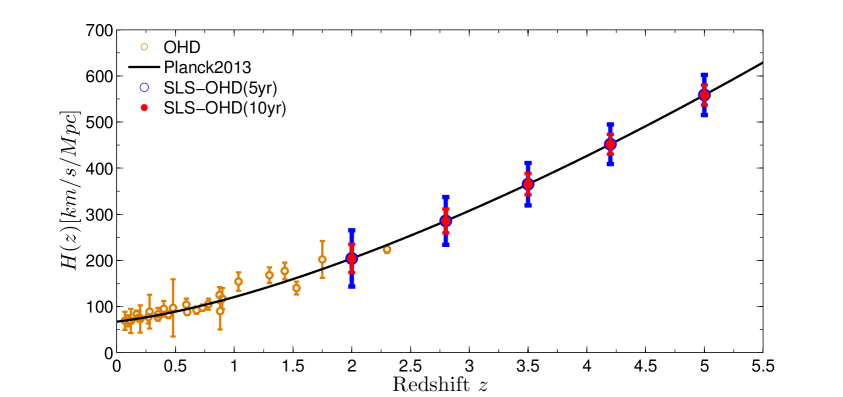
Therefore, the SL signal scheme can be used to extend the current OHD to a higher range of . This is a new method to measure the high redshift , and here we call it “SL signal scheme”. Note that the latest OHD contains 28 points and covers the region from to . The method described above can be used to complement the current OHD at higher redshifts.
Data
In the following analysis, we use the data model in Eq.(2.3) to make a forecast for a SL signal experiment on a CODEX-like survey. Namely, we consider a survey observing a total number of QSOs uniformly distributed in redshift bins of with of , by setting throughout this paper per redshift bin, i.e., 150 QSO in total. We consider a fiducial concordance CDM model to generate the mock data (the parameters have been set to the latest values obtained from the Planck analysis [20]), Then we use the mock data to examine the capability of the future OHD and check the improvement against current OHD. Both the forecast data and the current OHD are shown in Fig.1.
We have 2 ways to generate the simulated data using SL signal scheme. One way is to set the simulated data “directly” on the fiducial model like in the way used in [4] and [15]. This is only available under an ideal condition in which the observational values are not shifted away from the fiducial model predictions. Another way is to generate the mock data “shifted” from fiducial model by an offset :
| (2.4) |
where is just the fiducial model value. The offsets are stochastic variables from a Gaussian distribution
| (2.5) |
We choose the later one as the scheme to generate the mock data set “SL-OHD”.
Data Set Name Descriptions OHD The available OHD data (28 points). SL-OHD The mock Sandage-Loeb signal with offset . EOHD The “Extended OHD”: the combination set of OHD and SL-OHD.
The summary of mock data sets in this paper are listed in Table 1. The comparisons of constraining results are between OHD and EOHD. The duration of the SL experiment is yrs if not differently specified.
3 Test on Dark Energy Models
In this section, we focus on the potential improvement of high redshift OHD using the SL measurement strategy described in Eq.(2.3). Because of the possible non-gaussian posteriors in parameter space, we should perform a full MCMC analysis to explore the posterior distribution. Here we use the MCMC code PyMC [18] to sample the parameter space.
It has been shown in Eq.(2.3) that and are equivalent. However, there are some reasons and advantages that make the conversion of from meaningful:
-
•
The “SL signal scheme” we present in Sec.2 is a complete model independent measurement of . Because the SL signal is direct and independent against any pre-assumed model, extracted through SL scheme is a straightforward and directly comparable with the current 28 data points from ”cosmic chronometers”.
-
•
The overlapped redshift interval (around ) between current OHD and SL scheme OHD can be used for self-calibration for the values. The available OHD can be obtained up to , while the SL signal scheme can present a minimal redshift around 2. Hence the values retrieved from different methods will calibrate each other and enhance the accuracy at redshift around .
-
•
The current OHD observational methods are not efficient on derivating the values of in the redshift range of : only one point at is obtained so far. However, the SL signal scheme should be able to provide some values in this blank and break through the redshift bottleneck of OHD.
In this section we focus on the improvement of OHD on constraining the cosmological models after the introduction of the additional points obtained with the SL signal scheme. Namely, we compare the OHD with the EOHD (see Tab.1). We use OHD and EOHD to fit CDM and CDM models. For each model, we run MCMC sampling in its parameter space, finding the best fit values, confidence regions and convariance matrix. After we get these fitting quantities, the comparison between them should tell us the improvements and the capability of the SL signal scheme. They should be investigated from the following 3 aspects of statistical quantities from Markov chains: a) How much the errorbars can be reduced with the mock data? b) How does the Figure of Merit (FoM) changed? and c) What is the difference between the degeneracy of parameters of the mock data and OHD? The details about these aspects are explained in the following.
The relative accuracy improvement quality :
Suppose the current data can give marginalized 1- probability interval of the model parameter (the “error bar”) and our forecast data can give the new where is the th parameter of a given model. We can define the relative accuracy improvement quality :
| (3.1) |
Apparently, the larger positive the better the forecast data performs in constraining . We use this statistical quality to examine the improvement of the forecast data on a given parameter constraining.
The change of Figure of Merit (FoM) :
We follow the definition of DEFT (Dark Energy Task Force)[31] on the Figure of Merit (FoM):
| (3.2) |
where is the area of 1- confidence regions (or the so-called ”confidence ellipses”) of parameter and , is the 1- confidential interval of parameter and is the correlation coefficient between parameters and . The smaller is, the better constraint we get. For the current data, we can define the and for the forecast data we have . Therefore, the quantity FoM, defined as
| (3.3) |
tells us how the constraint from the forecast data is better than the current data in percentage.
The change of parameter degeneracy:
The degeneracy direction between and is determined by . Namely, we consider the covariance matrix of the parameter space :
| (3.4) |
where the correlation coefficient if . The covariance matrix can be estimated from the MCMCs. The difference between from the current and the forecast data tells us the change of the change of the degeneracy.
3.1 Standard Cosmological Model
In the CDM scenario, dark energy is constant in time, with an equation of state parameter According to the Friedmann equation, the prediction of Hubble parameter is
| (3.5) |
where . We perform the -statistics for this model:
| (3.6) |
where is the observational Hubble parameter data in the form of and is the theoretical prediction of Hubble parameters given by the cosmology. Therefore the model’s free-parameter vector is
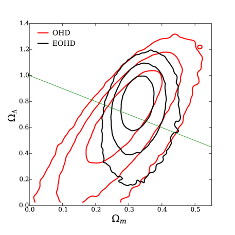
The capability of OHD and EOHD to constrain this model is shown in Fig.2 . We find that EOHD changes the direction of degeneracy significantly towards the vertical direction of the plane compared with the OHD which provides a better constraint. From the right panel of Fig.2, we find EOHD breaks the current degeneracy between and and produces a tighter constraints.
To illustrate the improvement of new data on constraining CDM quantitatively, we compare the marginalized probability distribution function of model parameters using Eq.(2). We find that in the case of CDM, the EOHD can improve all of the parameters with varies from 13.5% (for parameter ) to 58.5% (for parameter ).
Model OHD EOHD (%) CDM 4.45 3.85 13.5 0.08 0.03 58.5 0.25 0.15 40.0 0.32 0.18 43.7
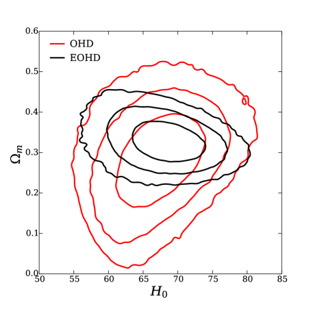
We can obtain the covariance matrix from the MCMC samples and extract the coefficient matrix which shows the degeneracy between parameters. The results are shown in Fig.(3) and is shown in Table 3.
Model OHD EOHD (%) CDM 128.64 274 112.59 4.32 8.13 88.66
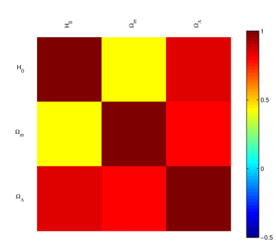
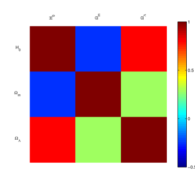
The comparisons just discussed imply that the 5 new mock data in EOHD obtained with the SL signal scheme can help to significantly improve the constraint on cosmological parameters.
3.2 CDM Scenario
Another widely studied model of dark energy is CDM parameterization where the dark energy is characterized by a constant equation of state parameter not necessarily equal to -1. The Friedmann equation in this model is:
| (3.7) |
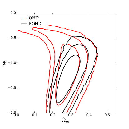
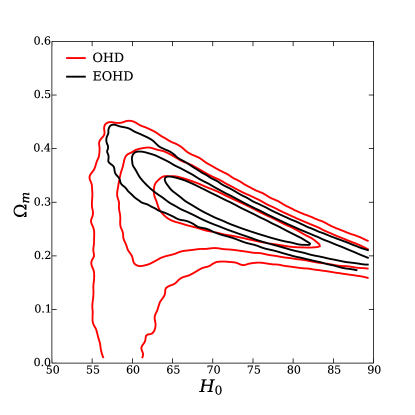
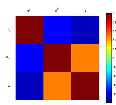
Here a flat universe is assumed i.e., The same statistics is performed using Eq.(3.6) with the free-parameter vector . The numerical results demonstrating the capability of OHD and EOHD to constrain this model are showed in Fig.4. We find that the contours in the - plane and in the plane presents strong degeneracies but the EOHD present a narrower and more elliptical region. Therefore the improvement of constraining is significant in (Table 5.) but weak in marginalized errorbars listed in Table 4: the improvement on is big () but not better on .
The comparison between OHD and EOHD under the CDM implied that the SL signal scheme do improve the quality of OHD and reduce the errorbars of parameters. The high redshift OHD have tiny effect on the , so the of is negligible. The quantitative description of the change of degeneracy is shown in Fig.(5).
Model OHD EOHD (%) CDM 5.84 5.80 0.68 0.04 0.04 -2.2 0.35 0.30 14.28
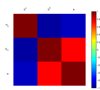
Model OHD EOHD (%) CDM 98.3 176 79 3.08 3.53 14.6
4 The Fisher matrix forecast on time-dependent
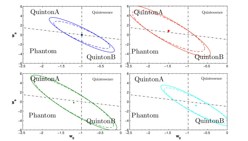
The dark energy is characterized by its equation of state, . Considering a changing as a function of redshift, , lots of models, such as Quintessence, phantom and Quintoms etc., are used to explain dark energy. Under the phenomenological parameterization like CPL parameterization [3, 11], the parameter plane can be divided into four blocks: the Quintom A, Quintom B, Phantom and Quintessence by lines and (see Fig.1 in [27]). Each of them refers to very different physical background. A question is then raised: can the future CODEX-like survey give measurement to distinguish these different models?
The Fisher matrix forecast is a powerful tool to answer this question. It is an approximation at first two terms of the likelihood, which is used for designing survey. The Fisher matrix in this work is defined as:
| (4.1) |
where is the value of OHD for a given cosmology :
| (4.2) |
The derivative values in Eq.(4.1) is obtained at the given fidicual cosmology .
To test if the SL OHD scheme can distinguish between different models, we perform the Fisher matrix forecast on these models. Here we take a more ambitious estimation on this future experiment: supposing that all QSO targets from SDSS DR7555For simplity, we suppose that all of these targets can be obsered by our survey. http://www.sdss.org/dr7/products/value_added/qsocat_dr5.html will be put into a 5-year SL signal experiment based on a CODEX-like survey, the number counts is in 7 redshift bins . Their errors can be obtained via Eq.(2.3) We pick up four points from plane: ()=(-1.5,0.8),(-1,0),(-1.2,-0.2) and (-0.8,0.8), fixing other cosmological parameters to be the same set-up as in previous sections. All of these four points are within the 3- regions of Plank analysis results [20]. The Fisher forecast are evaluated on these 4 models and results are shown in Fig.5. Comparing the solid ellipses(OHD) and the dotted ones(mix set of OHD and 7 forecast points) in Fig.5, we find that the improvements in the Figure of Merit (FoM) of corresponding models are real, but that are not sufficient to exclude the possibility of alternative dark energy models. Hence, the power to discriminate different dark energy models is weak, even considering such an optimistic forecast.
5 Conclusion and Discussions
In this paper we propose a new scheme to obtain the OHD in the redshift range of from the Sandage-Loeb signal by observing the Lyman- forest of QSOs. We simulated a CODEX-like survey, estimating new OHD points from SL signal at high redshifts as an addition to the current ones. The mixed data set of the current and the forecast data is called EOHD as a realistic forecast data of SL scheme. We analyzed the prospects for constraining dark energy models with EOHD, and compare the results with the current OHD.
The global fitting show that for CDM, comparing with OHD, all the errors on each single parameter are improved significantly(see Table.2) and the degeneracy between and is rotated to the vertical direction of the line (see Fig.3). The degeneracy between and is broken (see Fig.3). In the CDM case, we find that EOHD provides tighter constraints, with an improvement ratio for of 15.4.
The capability to distinguish the Quinton A, Quinton B, Phantom and Quintessence models from the plane under the CPL parameterization is also studied. Although the Fisher matrix forecast on the considered SL signal is quite optimistic, we found that it is still hard to distinguish these models clearly.
The Sandage-Loeb signal increases the available OHD redshift upper-limit significantly (from to ) and the SL signal scheme is conceptually simple and is a direct probe of cosmic dynamic expansion, though being observationally challenging. The data processing is also straightforward and there is no need of calibration step like in the case of type Ia SNe; e.g. obtained from the spectrum flux difference in this experiment between two different observational epochs will reduce the spectrum noise. Besides, the errors on data decrease linearly with observational time interval and can be significantly smaller over a few decades. It is hopeful to see small errors in the long enough observational interval.
Acknowledgments
We are grateful to Yingjie Peng, Hao-Ran Yu, Cong Ma, Feige Wang, and De-Zi Liu for helpful discussion. We also thank the anonymous referee whose suggestions greatly helped us improve this paper. This work was supported by the National Science Foundation of China (Grants No. 11173006), the Ministry of Science and Technology National Basic Science program (project 973) under grant No. 2012CB821804, the Fundamental Research Funds for the Central Universities.
References
- Balbi & Quercellini [2007] Balbi, A., & Quercellini, C. 2007, Mon. Not. R. Astron. Soc., 382, 1623, 0704.2350
- Blake et al. [2012] Blake, C. et al. 2012, Mon. Not. R. Astron. Soc., 425, 405, 1204.3674
- Chevallier & Polarski [2001] Chevallier, M., & Polarski, D. 2001, International Journal of Modern Physics D, 10, 213, arXiv:gr-qc/0009008
- Corasaniti et al. [2007] Corasaniti, P.-S., Huterer, D., & Melchiorri, A. 2007, Physics Review D, 75, 062001, astro-ph/0701433
- Eisenstein et al. [2005] Eisenstein, D. J. et al. 2005, Astrophys. J. , 633, 560, arXiv:astro-ph/0501171
- Farooq & Ratra [2013] Farooq, O., & Ratra, B. 2013, Astrophys. J. Lett., 766, L7, 1301.5243
- Gaztañaga et al. [2009] Gaztañaga, E., Cabré, A., & Hui, L. 2009, Mon. Not. R. Astron. Soc., 399, 1663, 0807.3551
- Jain & Jhingan [2010] Jain, D., & Jhingan, S. 2010, Physics Letters B, 692, 219, 0910.4825
- Li et al. [2013] Li, Z., Liao, K., Wu, P., Yu, H., & Zhu, Z.-H. 2013, Physics Review D, 88, 023003, 1306.5932
- Lin et al. [2009] Lin, H., Hao, C., Wang, X., Yuan, Q., Yi, Z.-L., Zhang, T.-J., & Wang, B.-Q. 2009, Modern Physics Letters A, 24, 1699, 0804.3135
- Linder [2003] Linder, E. V. 2003, Physical Review Letters, 90, 091301, arXiv:astro-ph/0208512
- Liske et al. [2008] Liske, J. et al. 2008, Mon. Not. R. Astron. Soc., 386, 1192, 0802.1532
- Loeb [1998] Loeb, A. 1998, Astrophys. J. Lett., 499, L111, arXiv:astro-ph/9802122
- Ma & Zhang [2011] Ma, C., & Zhang, T.-J. 2011, Astrophys. J. , 730, 74, 1007.3787
- Martinelli et al. [2012] Martinelli, M., Pandolfi, S., Martins, C. J. A. P., & Vielzeuf, P. E. 2012, Physics Review D, 86, 123001, 1210.7166
- McVittie [1962] McVittie, G. C. 1962, Astrophys. J. , 136, 334
- Moresco et al. [2012] Moresco, M. et al. 2012, J. Cosmology Astropart. Phys., 8, 6, 1201.3609
- Patil et al. [2010] Patil, A., Huard, D., & Fonnesbeck, C. J. 2010, Journal of Statistical Software, 35, 1
- Perlmutter et al. [1999] Perlmutter, S. et al. 1999, Astrophys. J. , 517, 565, arXiv:astro-ph/9812133
- Planck Collaboration et al. [2013] Planck Collaboration et al. 2013, ArXiv e-prints, 1303.5076
- Quercellini et al. [2012] Quercellini, C., Amendola, L., Balbi, A., Cabella, P., & Quartin, M. 2012, Physics Letters. B, 521, 95, 1011.2646
- Riess et al. [1998] Riess, A. G. et al. 1998, Astron. J., 116, 1009, arXiv:astro-ph/9805201
- Samushia & Ratra [2006] Samushia, L., & Ratra, B. 2006, Astrophys. J. Lett., 650, L5, astro-ph/0607301
- Sandage [1962] Sandage, A. 1962, Astrophys. J. , 136, 319
- Simon et al. [2005] Simon, J., Verde, L., & Jimenez, R. 2005, Physics Review D, 71, 123001, arXiv:astro-ph/0412269
- Stern et al. [2010] Stern, D., Jimenez, R., Verde, L., Stanford, S. A., & Kamionkowski, M. 2010, Astrophys. J. Suppl. Ser., 188, 280, 0907.3152
- Xia et al. [2008] Xia, J.-Q., Li, H., Zhao, G.-B., & Zhang, X. 2008, International Journal of Modern Physics D, 17, 2025, 0708.1111
- [28] Hao-Ran Yu, Shuo Yuan, and Tong-Jie Zhang. Nonparametric reconstruction of dynamical dark energy via observational hubble parameter data. Physical Review D, 88(10):103528, 2013.
- [29] Cong Zhang, Han Zhang, Shuo Yuan, Tong-Jie Zhang, and Yan-Chun Sun. Four new observational data from luminous red galaxies sloan digital sky survey data release seven. arXiv preprint arXiv:1207.4541, 2012.
- Zhang et al. [2010] Zhang, J., Zhang, L., & Zhang, X. 2010, Physics Letters B, 691, 11, 1006.1738
- [31] Albrecht, A. and Bernstein, G. et al. Four new observational data from luminous red galaxies sloan digital sky survey data release seven. astro-ph/0609591,2006