Supermassive Black Holes and Their Host Galaxies –
II. The correlation with near-infrared luminosity revisited

Abstract

We present an investigation of the scaling relations between Supermassive Black Hole (SMBH) masses, $M_{\bullet}$, and their host galaxies’ $K$-band bulge ($L_{\mathrm{bul}}$) and total ($L_{\mathrm{tot}}$) luminosities. The wide-field WIRCam imager at the Canada-France-Hawaii-Telescope (CFHT) was used to obtain the deepest and highest resolution near infrared images available for a sample of 35 galaxies with securely measured $M_{\bullet}$, selected irrespective of Hubble type. For each galaxy, we derive bulge and total magnitudes using a two-dimensional image decomposition code that allows us to account, if necessary, for large- and small-scale disks, cores, bars, nuclei, rings, envelopes and spiral arms. We find that the present-day $M_{\bullet}-L_{\mathrm{bul}}$ and $M_{\bullet}-L_{\mathrm{tot}}$ relations have consistent intrinsic scatter, suggesting that $M_{\bullet}$ correlates equally well with bulge and total luminosity of the host. Our analysis provides only mild evidence of a decreased scatter if the fit is restricted to elliptical galaxies. The log-slopes of the $M_{\bullet}-L_{\mathrm{bul}}$ and $M_{\bullet}-L_{\mathrm{tot}}$ relations are $0.75\pm 0.10$ and $0.92\pm 0.14$, respectively. However, while the slope of the $M_{\bullet}-L_{\mathrm{bul}}$ relation depends on the detail of the image decomposition, the characterization of $M_{\bullet}-L_{\mathrm{tot}}$ does not. Given the difficulties and ambiguities of decomposing galaxy images into separate components, our results indicate that $L_{\mathrm{tot}}$ is more suitable as a tracer of SMBH mass that $L_{\mathrm{bul}}$, and that the $M_{\bullet}-L_{\mathrm{tot}}$ relation should be used when studying the co-evolution of SMBHs and galaxies.

1. Introduction

The correlation between Supermassive Black Hole (SMBH) masses, $M_{\bullet}$, and the luminosities of their host galaxies’ bulges, $L_{\mathrm{bul}}$, is significant for at least two reasons.

First, there is to this date no obvious nor unique theoretical framework that satisfactorily explains its existence and characteristics (see, e.g., Shankar et al. 2012 and the discussion in Kormendy & Ho 2013). Understanding this, and other correlations between SMBHs and host galaxy properties, has important implications for understanding the origin of SMBHs and, possibly, the evolution of galaxies (e.g. Silk & Rees 1998; Cattaneo et al. 2006; Lusso & Ciotti 2011). Models of SMBH-galaxy co-evolution include mergers of galaxies and their SMBHs (e.g. Peng, 2007), but typically also invoke an interaction (“feedback”) between SMBHs and their hosts (e.g. Granato et al., 2004; Hopkins et al., 2006; Croton et al., 2006; Shankar et al., 2006; Volonteri et al., 2011; Fanidakis et al., 2012). The relative importance of mergers and feedback, their timescales, efficiencies and frequencies, may be constrained by comparing model predictions with the observed $M_{\bullet}-L_{\mathrm{bul}}$ relation.

Second, the $M_{\bullet}-L_{\mathrm{bul}}$ relation allows to infer SMBH masses, which are difficult to measure directly, from observationally much more accessible luminosities. This is used, for example, in the context of establishing the black hole mass function (BHMF) and its redshift evolution. Furthermore, the $M_{\bullet}-L_{\mathrm{bul}}$ relation derived from dynamically measured SMBH masses is also employed to calibrate methods of measuring $M_{\bullet}$ in active galaxies, namely reverberation mapping and secondary methods that are based on it (e.g. Onken et al., 2004; Ferrarese & Ford, 2005; McGill et al., 2008). The latter are frequently used to investigate the redshift evolution of SMBH masses and SMBH-galaxy scaling relations (e.g., Bennert et al., 2011).

The $M_{\bullet}-L_{\mathrm{bul}}$ relation shares both theoretical significance and predictive power with other correlations between SMBH mass and host galaxy properties, most notably the bulge stellar velocity dispersion, $\sigma_{\star}$, as well as stellar and dynamical mass, $M_{\mathrm{\star(,bul)}}$ and $M_{\mathrm{dyn(,bul)}}$. Of special interest in this context is the correlations’ intrinsic scatter, $\epsilon$, since a relation with low scatter allows a more precise estimate of $M_{\bullet}$, provided that the correlating quantity is observationally accessible with adequate precision. Yet, aside from desiring a “tight” relation as predictive tool, it is worthwhile to note that from a theoretical perspective, all correlations, not only the one with the lowest scatter, are of interest, since they serve as an additional constraint to evolutionary models. Consequently, it is imperative for the calibration of these relations to be as precise and unbiased as possible. For example, the models of Jahnke & Macciò (2011), where merging is the main driver behind the emergence of the $M_{\bullet}-M_{\star}$ relation at $z=0$, predict a lower scatter than observed unless star formation, black-hole accretion and disk-to-bulge conversion are included.

Unfortunately, the present characterization of the $M_{\bullet}-L_{\mathrm{bul}}$ relation and its intrinsic scatter are not secure. Published parameter values range from $\sim 0.9$ to $\sim 1.3$ for the log-slope, and $\sim 0.3$ to $\sim 0.6$ for the scatter $\epsilon$, with a typical $1\sigma$-uncertainty of $\sim 10\%$. Of particular interest is the relation at near-infrared (NIR) wavelengths, since, compared to optical, NIR luminosities are a better tracer of stellar mass and are less affected by dust extinction. The first study of $M_{\bullet}-L_{\mathrm{bul,NIR}}$ relations was based on 2MASS $J$, $H$ and $K$-band data (Marconi & Hunt, 2003, MH03 hereafter). The authors estimated the scatter in the relation, $\epsilon$, to be between 0.5 and 0.3, the former obtained using the full sample of $M_{\bullet}$ available at the time, the latter using a subsample of 27 galaxies deemed to have reliable estimates of $M_{\bullet}$. Surprisingly, MH03 found the intrinsic scatter in the NIR to be equivalent to the scatter in the optical ($B$-band) for the same sample, despite the expected advantages (less sensitivity to stellar population and dust effects) of working at longer wavelengths. Given the low resolution and depth of the 2MASS images, uncertainties in the bulge magnitudes derived from image decompositions can easily be underestimated, which would lead to overestimate the intrinsic scatter in the relation. This issue therefore demands further attention.

More recently, Vika et al. (2012, hereafter V12) presented an updated relation using data from the UKIDSS survey. The improved spatial resolution and depth of the data allowed them to account for nuclei, bars and cores when modeling galaxy images (while MH03 restricted their analysis to a bulge+disk decomposition). Based on a sample of 25 (19) galaxies, V12 found a characterization of the relation in agreement with MH03 (see Graham, 2007), but noted that the scatter increased to $~{}0.5\,\mathrm{dex}$ ($~{}0.4\,\mathrm{dex}$ for their restricted sample excluding barred galaxies), in spite of the clearly improved quality of the photometric data and analysis.

To further investigate the $K$-band $M_{\bullet}-L_{\mathrm{bul}}$ relation, we used the WIRCam instrument at CFHT to conduct a dedicated imaging survey, resulting in the deepest currently available homogeneous NIR-data set of known SMBH host galaxies with reliable direct $M_{\bullet}$ measurements. Since our goal is to perform an accurate decomposition of each galaxy into separate morphological components, we required $\lesssim 1\arcsec$ image resolution. In order to further reduce photometric uncertainties, we placed special emphasis on developing an observation strategy and data reduction pipeline that reliably accounts for the high and variable NIR background. Using the latest galfit profile fitting code (galfit3, Peng et al., 2010), we find that most galaxies require additional components in addition to a canonical bulge and (in most cases) disk, and demonstrate the large impact of the decomposition details on the derived bulge magnitudes. We additionally characterize the relation between $M_{\bullet}$ and total galaxy luminosity, $L_{\mathrm{tot}}$, and compare it with the $M_{\bullet}-L_{\mathrm{bul}}$ relation.

Details of the data acquisition and analysis, as well as a detailed discussion of each galaxy, are presented in a companion paper (Läsker et al. 2013, hereafter Paper-I). The present paper focuses on the derivation of the $M_{\bullet}-L$ scaling relations and is organized as follows: In §2 we describe the sample selection and summarize the analysis leading to our bulge and total luminosity measurements. §3 presents the ensuing scaling relations, including comparison with previous publications. We discuss our results in §4 and draw conclusions in §5. We elaborate on the correlation fitting method and the treatment of data uncertainties in the appendix.

2. Bulge and total luminosities from superior near-infrared imaging

2.1. Sample of SMBH host galaxies

Our sample comprises all galaxies visible from Mauna Kea for which a secure estimate of $M_{\bullet}$ had been published at the time our observing proposal was submitted (March 2008), regardless of Hubble type. “Reliable” $M_{\bullet}$ estimates are those derived based on dynamical modeling of the spatially resolved kinematics of gas or stars. We do not consider targets where only upper limits on $M_{\bullet}$ are available. In order to avoid systematic uncertainties implied by possibly unjustified model assumptions, we exclude galaxies for which $M_{\bullet}$ was derived from gas kinematics based on models with fixed disk inclination (e.g. NGC4459 and NGC4596, Sarzi et al. 2001), or from stellar kinematics based on isotropic dynamical models (NGC4594, Kormendy 1988; NGC4486b, Kormendy et al. 1997). Also excluded are measurements flagged as being particularly uncertain in the original papers (M31, Bacon et al. 2001; NGC1068 Greenhill et al. 1996; Circinus Greenhill et al. 2003, and the unpublished SMBH mass of NGC4742 (initially cited in Tremaine et al., 2002). NGC5128 (CenA) has been excluded because of declination constraints. Where available, we have adopted updated BH mass measurements that account for the DM halo (e.g. Schulze & Gebhardt, 2011), triaxiality (e.g. van den Bosch & de Zeeuw, 2010) and velocity dispersion of the gas disk (e.g. Walsh et al., 2010) in the model.

With respect to the work of MH03, we did not observe seven galaxies in their sample (M31, NGC1068, NGC4459, NGC4594, NGC4596, NGC4742 and NGC5128), although we note that $M_{\bullet}$ for four of these galaxies was also deemed of uncertain quality by MH03, and not included in their final analysis. Compared to V12, we did not observe five galaxies that are part of their final sample (NGC1068, NGC2960, NGC4303, NGC4459 and NGC4596), as well as four additional galaxies (NGC863, NGC4435, NGC4486b and UGC9799) that V12 also excluded from the fit as having uncertain $M_{\bullet}$. On the other hand, our study includes several galaxies that were not part of MH03’s nor V12’s analysis. Compared to MH03, we include seven galaxies for which $M_{\bullet}$ became available after their paper was published (IC4296, NGC1300, NGC1399, NGC2748, NGC3227, NGC3998, and PGC49940==A1836-BCG). None of these galaxies were part of the sample of V12; in addition, our sample contains 14 galaxies that were not analyzed by V12 (CygA, IC1459, NGC821, NGC1023, NGC2787, NGC3115, NGC3377, NGC3379, NGC3384, NGC3608, NGC4291, NGC5252, NGC6251 and NGC7457). Finally, we of course did not obtain a new measurement of the Milky Way bulge magnitude, and this galaxy is therefore not part of our final sample, in spite of its exceedingly well measured $M_{\bullet}$.

The above selection results in the sample of 35 galaxies listed in Table 2.1. The distances listed in the table are measured using Surface Brightness Fluctuations when available or otherwise estimated from the systemic velocity assuming $H_{0}=72\pm 8\,\textrm{km/s}$, (Freedman et al., 2001). All SMBH masses, which are taken from the literature, have been rescaled to the new adopted distances. Galactic foreground extinctions are taken from the NED database. $K$-band luminosities, as derived from our images, are also given (see Paper-I).

Table 1SMBH host galaxy sample

Galaxy	Hubble type	D [Mpc]	$M_{\bullet}~{}[10^{8}\,\,M_{\odot}]$	$\Delta M_{\bullet}~{}(+~{}/~{}-)$	$L_{K}~{}[10^{11}\,\,M_{\odot}]$	$R_{e}~{}[\mathrm{kpc}]$	Ref.
(1)	(2)	(3)	(4)	(5)	(6)	(7)	(8)
CygA	E	$238.0$	$26.5$	$6.4~{}/~{}6.4$	$13.2$	$19.6$	$2-1$
IC1459	E3	$28.4$	$24.4$	$2.8~{}/~{}2.8$	$3.71$	$3.98$	$1-2$
IC4296	E	$50.8$	$13.4$	$2.1~{}/~{}1.9$	$7.39$	$9.33$	$7-3$
NGC0221	cE2	$0.791$	$0.028$	$0.006~{}/~{}0.006$	$0.0133$	$0.124$	$1-4$
NGC0821	E6	$23.4$	$1.65$	$0.74~{}/~{}0.74$	$1.01$	$2.85$	$1-5$
NGC1023	S0	$11.1$	$0.42$	$0.04~{}/~{}0.04$	$0.944$	$1.92$	$1-6$
NGC1300	SBbc	$19.0$	$0.67$	$0.64~{}/~{}0.32$	$0.889$	$6.42$	$2-7$
NGC1399	E1pec	$21.2$	$5.1$	$0.7~{}/~{}0.7$	$3.89$	$5.72$	$8-8$
NGC2748	SAbc	$24.0$	$0.45$	$0.36~{}/~{}0.37$	$0.402$	$1.87$	$2-7$
NGC2778	S0	$22.3$	$0.129$	$0.1~{}/~{}0.1$	$0.174$	$1.07$	$1-5$
NGC2787	SB(r)0	$7.28$	$1.04$	$0.36~{}/~{}0.64$	$0.149$	$0.683$	$1-9$
NGC3115	S0	$9.42$	$8.85$	$2.8~{}/~{}2.8$	$1.03$	$1.63$	$1-10$
NGC3227	SAB(s)pec	$16.8$	$0.13$	$0.06~{}/~{}0.06$	$0.586$	$2.55$	$2-11$
NGC3245	SA0(r)?	$20.3$	$2.04$	$0.49~{}/~{}0.49$	$0.691$	$1.54$	$1-12$
NGC3377	E5	$10.9$	$1.77$	$0.93~{}/~{}0.93$	$0.312$	$1.47$	$1-5$
NGC3379	E1	$10.3$	$4.0$	$1.0~{}/~{}1.0$	$0.980$	$2.39$	$1-13$
NGC3384	SB(s)0-	$11.3$	$0.106$	$0.048~{}/~{}0.048$	$0.539$	$1.32$	$1-5$
NGC3608	E2	$22.3$	$4.55$	$0.97~{}/~{}0.97$	$0.854$	$2.67$	$1-5$
NGC3998	SA(r)0	$13.9$	$8.2$	$2.0~{}/~{}1.9$	$0.481$	$0.918$	$1-14$
NGC4258	SAB(s)bc	$7.21$	$0.39$	$0.01~{}/~{}0.01$	$0.768$	$3.03$	$4-15$
NGC4261	E2	$30.8$	$5.02$	$1.0~{}/~{}1.0$	$3.69$	$6.51$	$1-16$
NGC4291	E3	$25.5$	$9.37$	$3.0~{}/~{}3.0$	$0.728$	$1.78$	$1-5$
NGC4342	S0	$13.3$	$2.7$	$1.5~{}/~{}1.0$	$0.101$	$0.282$	$2-17$
NGC4374	E1	$18.5$	$9.27$	$0.98~{}/~{}0.87$	$3.34$	$5.25$	$5-18$
NGC4473	E5	$15.3$	$0.899$	$0.45~{}/~{}0.45$	$0.734$	$1.58$	$5-5$
NGC4486	E0pec	$16.7$	$61.5$	$3.7~{}/~{}3.7$	$4.54$	$7.18$	$5-19$
NGC4564	S0	$15.9$	$0.88$	$0.24~{}/~{}0.24$	$0.369$	$1.05$	$5-5$
NGC4649	E2	$16.4$	$47.1$	$10.0~{}/~{}10.0$	$3.94$	$5.16$	$5-20$
NGC4697	E6	$12.5$	$2.02$	$0.51~{}/~{}0.51$	$1.41$	$3.82$	$1-5$
NGC5252	S0	$97.3$	$10.0$	$15.0~{}/~{}4.7$	$3.20$	$3.97$	$2-21$
NGC5845	E*	$25.2$	$4.75$	$1.5~{}/~{}1.5$	$0.331$	$0.479$	$1-5$
NGC6251	E	$107.0$	$6.0$	$2.0~{}/~{}2.0$	$7.88$	$9.88$	$2-22$
NGC7052	E	$67.6$	$3.7$	$2.6~{}/~{}1.5$	$4.80$	$7.60$	$2-23$
NGC7457	SA(rs)0-	$12.9$	$0.092$	$0.055~{}/~{}0.055$	$0.205$	$1.86$	$1-5$
PGC49940	E	$153.0$	$37.6$	$4.3~{}/~{}5.2$	$7.67$	$12.3$	$2-3$

2.2. Data analysis and galaxy decomposition

Full details of the data reduction and analysis are given in Paper-I. All data were obtained with WIRCam at the Canada-France-Hawaii-telescope, have subarcsecond resolution (the median seeing on the final image stacks is $0\farcs 8$, a factor of 2-3 improvement over 2MASS), and signal-to-noise ratio of S/N=1 at $24\textrm{mag/arcsec}^{2}$, 4 and 2 mag deeper than 2MASS and UKIDSS, respectively. The observing strategy and data reduction were optimized to reduce both random and systematic uncertainty when subtracting the bright and highly variable NIR background.

Our measurements of apparent magnitudes are based on two-dimensional (2D) image decomposition performed with galfit3 (Peng et al., 2010), the details of which are given in Section 2 of Paper-I, which also includes a table listing bulge parameters and a discussion of the uncertainties associated with the models. To summarize, we require each galaxy model to contain a bulge with a Sérsic radial surface brightness profile (Sérsic, 1963). When warranted by the data, we also add a disk with exponential radial profile (equivalent to a Sérsic profile with index $n\equiv 1$). Such Sérsic bulge (+ exponential disk) models have been applied in most previous studies, and we refer to them as “standard” models.

After fitting all images with standard models, and measuring the corresponding bulge and total magnitudes, most (30 out of 35) galaxies showed characteristic residuals in the model-subtracted images. While large residuals are expected for spiral galaxies, we observe them in all galaxies with a disk component, and even in some ellipticals. This led us to attempt more detailed and complex models that include additional components (bars, nuclei, inner disks, envelopes, spiral arms), necessary profile modifications (such as diski-/boxiness and truncations) and masking the cores of giant ellipticals. We refer to these more complex models (i.e. including components in addition to bulge and disk) as “improved” models. To decide whether to include additional components as well as profile modifications in our analysis, we take a multi-prong approach, based on an examination of the radial profiles along the semimajor axis (obtained by IRAF ellipse), on the $\chi^{2}$ of the fit, and on a visual analysis of the residual image. We also verified the suitability of the fits by relaxing the assumption of an exponential profile for the disks. We required the models to be non-degenerate, and to converge to a best-fit with a stable minimum-$\chi^{2}$ that does not depend on the choice of initial parameters.

2.3. Bulge and total luminosities

An overview of the different definitions for the luminosities derived by applying standard and improved model decompositions is given in Table 2.

Table 2Definitions of Luminosities

Luminosity	Short name	Definition
$L_{\mathrm{b,std}}$	“standard bulge”	bulge component luminosity from a standard Sérsic-bulge(+exponential disk) model
$L_{\mathrm{b,min}}$	“minimal bulge”	bulge component luminosity from an improved (additional components or masked core) model
$L_{\mathrm{b,max}}$	“maximal bulge”	total minus disk and (if present) spiral arm luminosity of the improved model
$\boldsymbol{L_{\mathrm{sph}}}$	“spheroid”	luminosity of bulge component plus envelope (if present) in the improved model
$L_{\mathrm{ser}}$	“Sérsic”	luminosity of single-Sérsic models (all galaxies)
$L_{\mathrm{t,std}}$	“standard total”	sum of bulge and disk luminosity of a standard model
$\boldsymbol{L_{\mathrm{t,imp}}}$	“improved total”	sum of all component luminosities from an improved model
$L_{\mathrm{24}}$	“isophotal”	luminosity within aperture delimited by the $24\,\mathrm{mag\,arcsec^{-2}}$ isophote
$L_{\{\cdot\}}^{\mathrm{(ell)}}$	“ellipticals”	luminosities of elliptical galaxies

For all galaxies, we measure $L_{\mathrm{b,std}}$, the luminosity of the bulge component in a “standard” bulge(+disk) model. For galaxies requiring components in addition to a bulge and disk, we derive three distinct improved bulge luminosities: the “minimal” bulge luminosity ($L_{\mathrm{b,min}}$) is the luminosity of the improved model’s bulge component alone; the “maximal” bulge luminosity is derived by summing the flux of all components except the disk and, if present, spiral arms. Therefore, $L_{\mathrm{b,min}}$ constitutes a lower, and $L_{\mathrm{b,max}}$ an upper limit estimate for the bulge luminosity. $L_{\mathrm{b,min}}$ and $L_{\mathrm{b,max}}$ sometimes differ considerably from one another, as well as from $L_{\mathrm{b,std}}$. For several galaxies, the latter is outside of the range defined by $L_{\mathrm{b,min}}$ and $L_{\mathrm{b,max}}$, indicating that a blind bulge+disk decomposition can significantly bias the results. A final estimate of the bulge luminosity, the “spheroid luminosity” ($L_{\mathrm{sph}}$), includes the flux of the envelope component, in addition to the bulge component (see §3.3 of Paper-I). As detailed in Paper-I, interpretation of the envelope is not straightforward, but it most likely represents part of the spheroidal stellar distribution, which is not well fit by a single 2D-Sérsic profile. This of course applies only to galaxies in which such an envelope is identified and required to obtain a suitable fit; for all other targets, $L_{\mathrm{sph}}=L_{\mathrm{b,min}}$.

Combining the luminosities of all components provides the total luminosity, $L_{\mathrm{t,std}}$ and $L_{\mathrm{t,imp}}$, of the standard and improved model, respectively. Naturally, for elliptical galaxies (fit by a single Sérsic profile), the total equals the bulge luminosity. If the galaxy has a core (defined as a deficit of light relative to the inner extrapolation of the Sérsic law that best fits the outer parts of the profile, e.g. Ferrarese et al. 2006), the core is masked and the total luminosity obtained is $L_{\mathrm{t,imp}}$; for all other ellipticals, also $L_{\mathrm{t,imp}}=L_{\mathrm{t,std}}$. In order to examine the effect of omitting any sub-components (including the exponential disk) from the model, as may occur in circumstances of insufficient image depth or resolution, we supply also the (total) luminosity from fitting single Sérsic profile to all galaxies ($L_{\mathrm{ser}}$). In addition, we derive a non-parametric luminosity from aperture photometry. The resulting isophotal luminosity, $L_{\mathrm{24}}$, accounts for the flux inside $R_{24}$, the radius at which the surface brightness drops below $24\,\mathrm{mag\,arcsec^{-2}}$. Differences between $L_{\mathrm{t,std}}$, $L_{\mathrm{t,imp}}$ and $L_{\mathrm{24}}$ are relatively small compared to the variance between the various definitions of bulge luminosities.

Although standard models rarely provide a good description for the data, they are useful to investigate the impact that the modeling complexity has on the BH scaling relations. Of course, in galaxies where a bulge(+disk) model suffices and no core is present (1 lenticular and 8 elliptical galaxies for our sample), we adopt luminosities from the standard model throughout. All luminosities are given in units of solar luminosity and have been converted from the absolute magnitudes given in Table 2 of Paper-I using the absolute $K$-band magnitude of the Sun, $M_{K,\odot}=3.28$.

In summary (see Table 2), we have four estimates for the bulge luminosity, $L_{\mathrm{bul}}=\{L_{\mathrm{b,std}},~{}L_{\mathrm{b,min}},~{}L_{\mathrm{b,max}},~{}L_{\mathrm{sph}}\}$, and four estimates for the total luminosity, $L_{\mathrm{tot}}=\{L_{\mathrm{ser}},~{}L_{\mathrm{t,std}},~{}L_{\mathrm{t,imp}},~{}L_{\mathrm{24}}\}$. $L_{\mathrm{b,std}}$ and $L_{\mathrm{t,std}}$ are derived using a “standard” model (bulge plus, if needed, disk), while $L_{\mathrm{b,min}}$, $L_{\mathrm{b,max}}$, $L_{\mathrm{sph}}$ and $L_{\mathrm{t,imp}}$ are derived from improved models that include additional components. By contrast, $L_{\mathrm{24}}$ is a parameter-free measurement of total luminosity.

Table 3Luminositiy values

3. Resulting scaling relations

For all sample galaxies, we plot the luminosities, $\tilde{L}_{\{\cdot\}}=\log\left(L_{\{\cdot\}}/\,L_{\odot}\right)$ against SMBH mass, $\tilde{M_{\bullet}}\equiv\log\left(M_{\bullet}/\,M_{\odot}\right)$, and fit a correlation with a ridgeline

$$\tilde{M_{\bullet}}=a+b(\tilde{L}_{\{\cdot\}}-11)~{},$$ (1)

including a Gaussian intrinsic scatter $\epsilon_{\bullet}$ in the direction of $\tilde{M_{\bullet}}$ (y-axis) and $\epsilon_{\bot}$ in the direction perpendicular to the ridgeline. The subscript indicates one of the choices described in §2.3 and Table 2.3. The corresponding $\tilde{M_{\bullet}}$ and $\tilde{L}$ values are listed in Table 2.3. We choose to pivot all relations around $L=10^{11}\,L_{\odot}$ since this value is approximately equal to the mean luminosity of the sample, reducing the covariance between $a$ and $b$. In the remainder of this section, we use the notation $\epsilon\equiv\epsilon_{\bullet}$, as opposed to $\epsilon_{\bot}$. We also introduce the shorthand notation $\{p\}_{\{\cdot\}}^{\mathrm{(ell)}}$, where $p\in\{a,b,\epsilon\}$ may be any of the fit parameters, the subscript again indicates the type of luminosity measurement used, and the superscript (ell) is present if only elliptical galaxies were used in fitting the relation.

The parameter estimates are performed by calculating the three-dimensional posterior probability distribution of the parameters $(a,b,\epsilon)$ on a dense grid. The maximum of the likelihood function corresponds to the adopted parameters, while the quoted uncertainties correspond to the central 68%-confidence interval of the marginalized distributions. We supplement our statistical analysis by estimates from bootstrap-resampling and find the results to be consistent. For more details on the choice of the fitting method, and the treatment of uncertainty in the data, please see Appendix A. A summary of the parameters derived for all fitted scaling relations is given in Table 3.

Table 4Resulting scaling relations

3.1. Bulge versus total luminosity

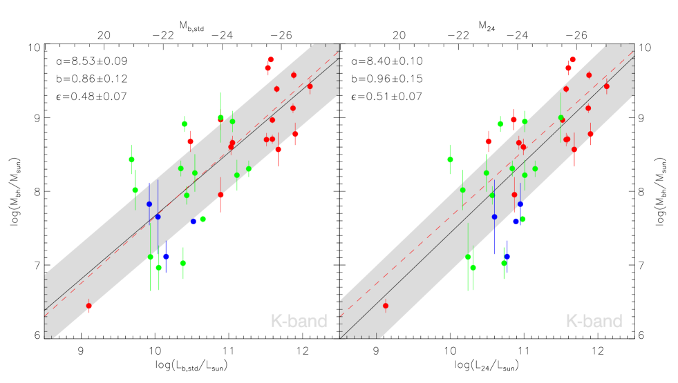
Figure 1.— Correlation between $M_{\bullet}$ and “standard” bulge ($L_{\mathrm{b,std}}$ left panel) and non-parametric isophotal ($L_{\mathrm{24}}$, right panel) luminosity. The filled circles correspond to elliptical (red), S0 (green) and spiral (blue) galaxies. Vertical solid bars indicate the $1\sigma$-uncertainties in $M_{\bullet}$. The black solid lines are the corresponding best-fit linear relations of the form $\log M_{\bullet}=a+b(\log L-11)$. The shaded area has a width of $2\epsilon_{\bullet}$ in the direction of $M_{\bullet}$. As expected, the best-fit slope $b$ is steeper for total luminosities. Crucially, the intrinsic scatter $\epsilon$ of both relations is the same. The red dashed lines are the relations fitted to the sample of elliptical galaxies only (see §3.1 and Table 3).

Comparing how $M_{\bullet}$ correlates with $L_{\mathrm{bul}}$ and $L_{\mathrm{tot}}$ in the $K$-band, we find three significant results:

1. bulge and total luminosities lead to similarly tight correlations with comparable intrinsic scatter;

2. the log-slope of the $M_{\bullet}-L_{\mathrm{bul}}$ relation is significantly less than unity, while the $M_{\bullet}-L_{\mathrm{tot}}$ relation is consistent with being linear; and

3. the characterization of the $M_{\bullet}-L_{\mathrm{tot}}$ relation is robust against the choice of method used in deriving $L_{\mathrm{tot}}$. This is not the case for the $M_{\bullet}-L_{\mathrm{bul}}$ relation.

These results hold regardless of the method used to derive the luminosity (standard/improved models or curve-of-growth analysis). Points (i) is highlighted in Figure 1 using $L_{\mathrm{b,std}}$ and $L_{\mathrm{24}}$, as these represent the simplest available estimates of bulge and total luminosity, respectively. Figure 2 illustrates point (iii), i.e. the dependency of the $M_{\bullet}-L_{\mathrm{bul}}$ relation on the details of the photometric decomposition, which causes large (and not easily quantifiable) uncertainties in the bulge photometry. Finally, confirming (i) and demonstrating result (ii), Figure 3 displays our adopted (preferred) $M_{\bullet}-L_{\mathrm{sph}}$ and $M_{\bullet}-L_{\mathrm{t,imp}}$ relationships based from our improved decompositions.

The intrinsic scatter does not seem to depend on which choice of luminosity is adopted in defining the relations. In particular, the scatter found using bulge luminosities derived from the “standard” model, $\epsilon_{\mathrm{b,std}}=0.48^{+0.10}_{-0.04}$, is virtually identical to the one obtained when using bulge luminosities from the “improved” models, whether they are the minimum (i.e. bulge alone), maximum (i.e. bulge plus additional components except the disk and spiral arms), or ”spheroidal” (bulge plus envelope) estimates (see §2.2). This is somewhat surprising, given that the improved models generally do a significantly better job than standard models at reproducing the structure seen in many of our sample galaxies (see Paper-I).

If total magnitudes are used, likewise all choices of luminosity lead to $\epsilon_{\mathrm{tot}}\approx 0.5$, again consistent with $\epsilon_{\mathrm{b,std}}$. In other words, no matter whether bulge or total magnitudes are used, and regardless of the specifics of the decomposition or photometric analysis, all $\epsilon$ agree at the 68%-confidence level. The same applies when one considers $\epsilon_{\bot}$, the scatter perpendicular to the ridge line (see Table 9). Both $\epsilon_{\bullet}$ and $\epsilon_{\bot}$ decrease when the fit is restricted to elliptical galaxies, but the difference is not significant beyond the $1\sigma$-confidence level.

While the scatter does not seem to be sensitive to the details of the photometric analysis, the characterization of the relation, in particular its slope, does, but only when bulge luminosities are used. When using total luminosity, all $M_{\bullet}-L_{\mathrm{tot}}$ relations agree closely in slope, $b_{\mathrm{tot}}$, irrespective of the method used to obtain $L_{\mathrm{tot}}$. The slopes of the $M_{\bullet}-L_{\mathrm{bul}}$ relations obtained from the improved models, $b_{\mathrm{b,min}}$ and $b_{\mathrm{sph}}$, are smaller than $b_{\mathrm{tot}}$ at the $1\sigma$-confidence level. This is to be expected: while the high mass end is dominated by elliptical (i.e. pure bulge) galaxies, bulges comprise only a fraction of the total luminosity in the (on average less luminous) lenticular and spiral galaxies. $b_{\mathrm{bul}}$ increases when maximum bulge magnitudes or standard decompositions are used, such that $b_{\mathrm{b,max}}$ and $b_{\mathrm{b,std}}$ are consistent with $b_{\mathrm{tot}}$ and $b^{\mathrm{(ell)}}$.

Using improved decompositions (Figure 3), the slope of the $M_{\bullet}-L_{\mathrm{tot}}$ relation remains virtually unchanged whether all galaxies, or only ellipticals are fitted. Consequently, the slope of the $M_{\bullet}-L_{\mathrm{bul}}$ relation ($L_{\mathrm{bul}}=L_{\mathrm{sph}}$), when fitted to the entire sample, is also systematically smaller (at the $\sim 1\sigma$ confidence level) than the slope fitted to the sample of ellipticals only, $b^{\mathrm{(ell)}}$. Yet, $b^{\mathrm{(ell)}}$ should be treated with caution, since it is very sensitive to a specific galaxy, NGC221 (M32), the only elliptical in our sample with $L\lesssim 10^{11}\,L_{\odot}$ and $M_{\bullet}\lesssim 10^{8}\,M_{\odot}$. Therefore, we view the evidence that the slope of the $M_{\bullet}-L_{\mathrm{bul}}$ relation depends on Hubble type as tentative at best.

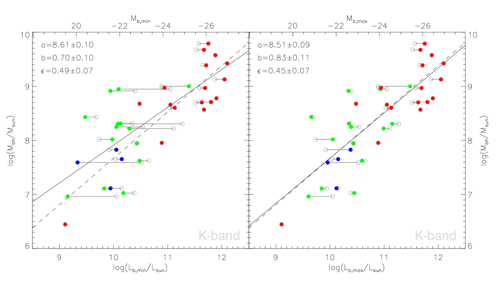
Figure 2.— Correlations of $M_{\bullet}$ with improved models’ minimal ($L_{\mathrm{b,min}}$, left panel) and maximal ($L_{\mathrm{b,max}}$, right panel) bulge luminosities. Filled circles, error bars and black solid lines are as defined in Figure 1. Overplotted in gray are the standard bulge values (open circles), while the dashed line is the corresponding $M_{\bullet}-L_{\mathrm{b,std}}$-relation. Error bars in $M_{\bullet}$ have been omitted for clarity, but are the same as in Fig. 1. Note that, somewhat unexpectedly, the $M_{\bullet}-L_{\mathrm{b,max}}$-relation is consistent with the $M_{\bullet}-L_{\mathrm{b,std}}$ relation. The figure also illustrates the changes in bulge luminosity as a consequence of applying a detailed decomposition. Notably, some $L_{\mathrm{b,min}}$ are larger than $L_{\mathrm{b,std}}$, while some $L_{\mathrm{b,max}}$ are smaller than $L_{\mathrm{b,std}}$. One also sees the effect of cores in elliptical galaxies (red circles), which are masked when obtaining $L_{\mathrm{b,min}}$ and $L_{\mathrm{b,max}}$.

3.2. The adopted scaling relations

Our recommendation is to use $M_{\bullet}-L_{\mathrm{bul}}$ scaling relations based on “improved model” fits to the $K$-band images. The rationale for introducing galaxy image models that improve on the “standard” bulge(+disk) configuration are described in Paper-I. In short, they are warranted by considerable and characteristic mismatches between data and standard models, with residuals usually revealing bars, galactic nuclei (AGN or clusters), inner disks and spiral arms. Such components are often easily identified by visually inspecting the science image. They are known to be morphologically and kinematically distinct from the spheroidal (“hot”) stellar component and should therefore be excluded when characterizing the properties of the latter. Such considerations do not apply to elliptical galaxies, although we note that masking the cores in core-Sérsic galaxies (e.g. Ferrarese et al., 2006) improves the luminosity estimate, eliminating the bias induced by the Sérsic profile’s mismatch in the central region.

As for which estimate of the bulge luminosity to use, our preference is for $L_{\mathrm{sph}}$, the luminosity of the bulge component plus, when present, an additional spheroidal envelope, for the following reasons. $L_{\mathrm{b,max}}$ does not measure the luminosity of the bulge/spheroidal component, but of all components except the disk and spiral arms. It therefore marks an upper limit for $L_{\mathrm{bul}}$ and was introduced primarily to compare results from standard and improved models. $L_{\mathrm{b,max}}$ would be the “proper” luminosity only if one assumed that the extra components (such as bars and stellar nuclei) are not separate entities but are instead part of the bulge. By contrast, $L_{\mathrm{b,min}}$ is the luminosity of the central component with Sérsic index $n>1$ and higher axis ratio than the disk(s), and therefore corresponds to the commonly adopted photometric definition of “bulge”. As described in Paper-I, for five of our galaxies this definition probably does not describe the spheroidal (“hot”) stellar component entirely. Instead, an “envelope” component is required for suitable image modeling and should be added to $L_{\mathrm{b,min}}$ in order to measure the luminosity of the spheroid, $L_{\mathrm{sph}}$ (we note that the physical nature of such envelope is not clear – it might simply be part of the bulge, or even an artifact introduced by the choice of parametrization for the bulge and the disk, see the discussion in Paper-I). Therefore, interpreting the term “bulge” in the sense of “spheroid”, we adopt the correlation of $M_{\bullet}$ with $L_{\mathrm{sph}}$, rather than $L_{\mathrm{b,min}}$, as the best available characterization of $M_{\bullet}-L_{\mathrm{bul}}$.

When using total luminosity, we also prefer values derived from improved models, for the same reasons given above, although we note that correlations with total luminosities from standard models and aperture photometry lead to virtually identical correlation parameters. The $K$-band $M_{\bullet}-L_{\mathrm{sph}}$ and $M_{\bullet}-L_{\mathrm{t,imp}}$-relations are highlighted in Tables 2, 3 and A.4, and plotted in Figure 3.

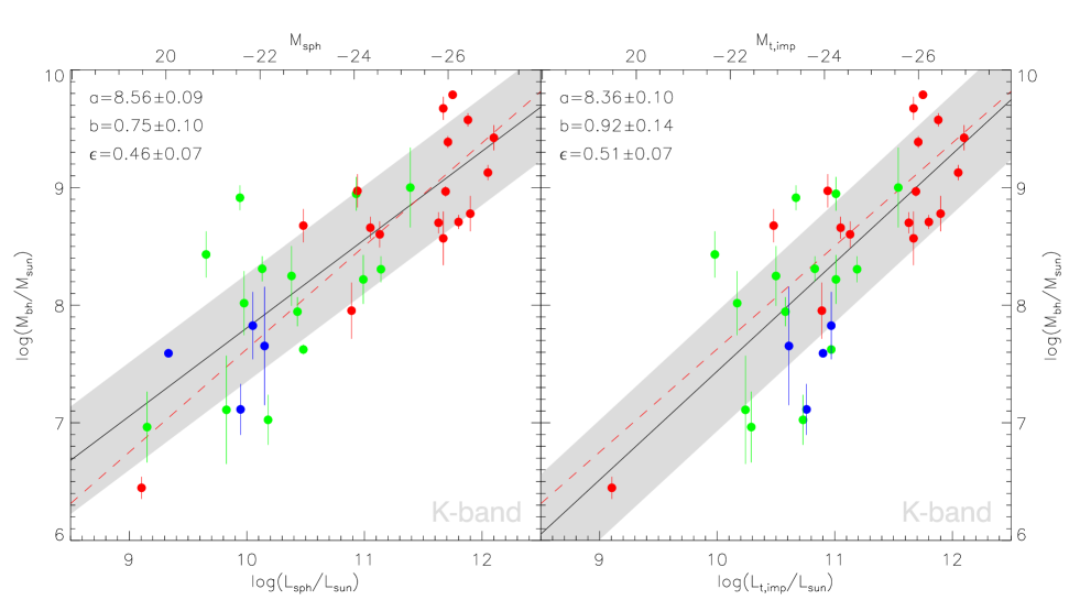
Figure 3.— Our adopted correlations of $M_{\bullet}$ with bulge/spheroid ($L_{\mathrm{sph}}$, left panel) and total ($L_{\mathrm{t,imp}}$, right panel) luminosity. Filled colored circles, error bars and lines are defined as in Figure 1. The respective intrinsic scatter is indicated by the shaded area, which has a width of $2\epsilon_{\bullet}$ in the direction of $M_{\bullet}$. Note the similar scatter of the two relations, as well as the similarity between the slopes of $M_{\bullet}-L_{\mathrm{t,imp}}$ and the fit to ellipticals only, $M_{\bullet}-L_{\mathrm{imp}}^{\mathrm{(ell)}}$ (red dashed line in both panels).

3.3. Comparison with previous studies

Table 5Comparison with previous studies

In Table 3.3, we compare our results (bottom line) with those from previous studies that investigated the $K$-band $M_{\bullet}-L_{\mathrm{bul}}$ scaling relation (lines 1-8). We also include in the comparison the relation of Sani et al. (2011) [S11 hereafter], which was derived at $3.6\mu\mathrm{m}$.

Our zero-point ($a=8.56\pm 0.09$) is consistent with the value measured by V12, but is higher than that of MH03 and, in particular, Graham (2007) [G07 hereafter], who re-fitted the data from MH03 after revising a number of $M_{\bullet}$ and distance values, and removing five galaxies from MH03’s sample of reliable $M_{\bullet}$ measurements. The results of MH03 and G07 were both based on 2MASS data (G07 relied on the 2D fits of MH03), which is inferior, both in spatial resolution and depth, to our data or the UKIDSS data used by V12. In Paper-I, we show that using data with low S/N or spatial resolution typically leads to overestimate the bulge luminosities, and speculate that this may explain the lower zero-point resulting from 2MASS data.

Our log-slope, $b_{\mathrm{sph}}=0.75\pm 0.10$, is shallower than found in all previous studies. The difference is above the $1\sigma$-level, and again the smallest difference is found with respect to the V12 estimate. The comparison suggests a general trend towards shallower slope with increasing data quality and decomposition complexity. G07 obtains a shallower slope than MH03, presumably in part a result of separating the disk from the bulge in three galaxies to which MH03 applied a single Sérsic profile. In contrast to MH03 and G07, the resolution and depth of the data allowed S11 and V12 to also model nuclei and bars, and they find a (slightly) shallower slope than G07. V12 also accounted for cores, and their result yields $b<1$ at the $1\sigma$-confidence level. Our slope is shallower still, possibly due to further improved bulge photometry, which typically reduces the luminosity estimate at the lower-mass end (predominantly late Hubble type) and increases it for some of the ellipticals.

We note that the choice of fitting method also plays a role, as expected (e.g., Novak et al., 2006): When fitting the same data ($L_{K}$ and $M_{\bullet}$) as used by MH03 (their Table 1) with our likelihood method (lines 2 and 4 of Table 3.3), the resulting slopes are shallower than the relation reported by MH03 (bisector estimator of Akritas & Bershady, 1996, lines 1 and 3), although they are still significantly steeper than the relations derived in this paper.

As for the scatter, we again are in agreement with the result V12, deriving a larger $\epsilon$ than either MH03 (for their ”group 1” sample) or G07, despite using improved data and decompositions. The scatter derived by S11 using $3.6\,\mu\mathrm{m}$ data also agrees more closely with ours, although it is important to keep in mind that both S11 and V12 use samples and sample selection criteria that are different from one another and from our study. S11 exclude pseudobulges identified based on the bulge’s Sérsic index, which may be highly uncertain and subject to the modeling complexity (see Paper-I). V12 exclude barred galaxies, M87 (due to concerns about the background subtraction) and an outlier, NGC4342. Irrespective of the suitability of the applied criteria to identify pseudobulges / barred galaxies, and the astrophysical justification to exclude such objects from the analysis, these sample restrictions are expected to decrease the scatter, since by construction they do not apply to elliptical galaxies, and (presumably) only rarely to early-type lenticulars. That is, they tend to bias the sample towards early-type and luminous galaxies, for which numerous studies (including ours) find a slightly decreased scatter. Indeed, V12 find a marginally higher scatter ($0.52^{+0.10}_{-0.06}$ instead of $0.40^{+0.09}_{-0.06}$) when analyzing their full sample of reliable $M_{\bullet}$ (line 5 in Table 3.3), higher than the scatter of our adopted $M_{\bullet}-L_{\mathrm{sph}}$ relation ($0.42^{+0.08}_{-0.04}$).

To investigate how the choice of decomposition affects the slope, normalization, and scatter of the relation, we extract a sample in common between ours and MH03’s, and derive scaling relations for this sample using both our data and MH03’s (lines 9-12 in Table 3.3). Using MH03’s black hole masses and luminosities, but restricting the sample to the common objects (from 37 to 28 galaxies, compare lines 2 and 9) leaves the slope $b$ unchanged, but increases the normalization $a$ and decreases the scatter $\epsilon$ at the 1$\sigma$ level (compare line 9 to line 2 in table 3.3). We then replace the $M_{\bullet}$ that MH03 used with our updated values (line 10), and find little effect on $b$ and $\epsilon$, but a significantly increased zero-point. If we use the same $M_{\bullet}$ as MH03, but replace the MH03 luminosities with our improved $L_{\mathrm{sph}}$ (line 11), the zero point also increases, but not quite as much. At the same time, $b$ and $\epsilon$ decrease by $0.11$ and $0.04\,\mathrm{dex}$, comparable to the change we observed when replacing standard bulge luminosities ($L_{\mathrm{b,std}}$) with $L_{\mathrm{sph}}$ while fitting our (full) sample. Using both improved $L_{\mathrm{sph}}$ and updated $M_{\bullet}$ (line 12, compared to line 9) combines the above effects (increased $a$, decreased $b$, slightly decreased $\epsilon$) and leads to a best-fit relation that is in close agreement with our adopted relation (our full sample, line 13). Therefore, the above analysis confirms that accounting for components beyond the bulge and the disk (as done in our study but not in MH03) is the dominant driver towards a shallower slope, while the updated $M_{\bullet}$ estimates are the main (but not sole) cause for the higher zero-point of our relation relative to that of MH03. Meanwhile, the intrinsic scatter appears to be primarily effected by sample selection and decreases only slightly when using improved bulge luminosity estimates.

4. DISCUSSION

4.1. The theorist’s perspective

Our analysis suggests that $M_{\bullet}$ correlates as tightly with $L_{\mathrm{tot}}$ as it does with $L_{\mathrm{bul}}$. This is evidenced by the fact that the intrinsic scatter (whether it is measured along the $M_{\bullet}$ axis or orthogonal to the relation) for the two relations is comparable: for instance, along the $M_{\bullet}$ axis, $\epsilon_{\mathrm{bul}}=0.46^{+0.09}_{-0.04}$ while $\epsilon_{\mathrm{tot}}=0.51^{+0.10}_{-0.04}$ (lines 4 and 7 of Table 3). This result challenges the view that SMBHs do not scale as tightly (or at all) with the total galaxy luminosity, as first argued by Kormendy & Gebhardt (2001) based on $B-$band data from a non-identified source. The use of $B-$band luminosity, however, is not-ideal to address this issue, at least if it is assumed that mass, rather than luminosity, might be the primary driver for the relations. Subsequent studies have, therefore, correctly focused on luminosities derived at longer wavelengths. Beifiori et al. (2012), using $i-$band data, state that “bulge luminosity is a better tracer of the mass of the SMBHs than total light of the galaxy”. However, this claim seems to be contradicted by their Table 5, which shows that the intrinsic scatter in the relation using bulge magnitudes ($0.58\pm 0.11$ for their sample ”B”) is, at face value, larger than the scatter in the relation using total magnitudes ($0.52\pm 0.11$). The total scatter of both relations is consistent in all samples used by Beifiori et al. (2012), and similarly when luminosities are replaced by the respective stellar or dynamical mass.

The connection between $M_{\bullet}$ and total stellar mass, $M_{\star,\mathrm{tot}}$ (and implicitly its surrogate, $L_{\mathrm{tot}}$), has been the subject of studies investigating BH scaling relations for active galaxies and their evolution with redshift (e.g. Kim et al., 2008; Merloni et al., 2010; Bennert et al., 2011; Cisternas et al., 2011), and some have suggested that it might represent a comparable or even tighter correlation than $M_{\bullet}-M_{\mathrm{bul}}$ (Peng, 2007; Jahnke et al., 2009; Bennert et al., 2010). Our result provides a local baseline for these studies, with the caveat that it is based on quiescent galaxies and different $M_{\bullet}$ measurement methods. It further seems to support the idea that SMBH growth may be linked with the overall potential of the host (as in Ferrarese, 2002; Volonteri et al., 2011), as traced by its total NIR luminosity (stellar mass). This is also in line with the evidence that, at fixed radiative efficiency, the integrated accretion history of SMBHs, as traced by active galactic nuclei, parallels the full star formation history of SMBH host galaxies (e.g., Shankar et al., 2009). An $M_{\bullet}-M_{\star,\mathrm{tot}}$ relation with scatter similar to that of $M_{\bullet}-M_{\star,\mathrm{bul}}$ is also predicted by the merger-driven models of Jahnke & Macciò (2011). We note however that, if repeated sequences of galaxy mergers have characterized the growth of spheroids and disks, and have been strictly accompanied by mergers of their central SMBHs, the ensuing relations should become tighter for elliptical (and more massive) galaxies, while we observe only a modest decrease. However, firm conclusions on this point must await larger samples of both early and late type galaxies, spanning a wider mass range than the present sample.

Our results for the correlation slope and offset also impact our current understanding of the connection between SMBH and host galaxy. The slope we obtain for (the logarithm of) the $M_{\bullet}-L_{\mathrm{bul}}$ relation, $b_{\mathrm{bul}}=0.75\pm 0.10$, excludes a direct proportionality between $M_{\bullet}$ and bulge stellar mass, $M_{\star,\mathrm{bul}}$, with high confidence. Assuming that the $K$-band stellar mass-to-light ratio, $M_{\star}/L_{K}$, is on average positively correlated with $L_{K}$, the log-slope of the $M_{\bullet}-M_{\star,\mathrm{bul}}$ relation is even lower than $b_{\mathrm{bul}}$, which is already $<1$ with $\gtrsim 99\%$ confidence according to our study. Combining our $M_{\bullet}-L_{\mathrm{bul}}$ relation with, for example, $\log M_{\star}\propto(1.12\pm 0.02)\times\log L_{K}$ (Zhu et al., 2010), a simple estimate yields $\log M_{\bullet}\propto(0.67\pm 0.11)\log M_{\star,\mathrm{bul}}$. That is, the $M_{\bullet}/M_{\star,\mathrm{bul}}$-ratio decreases with host bulge/spheroid mass. This is in agreement with Sani et al. (2011), who found $b_{\star,\mathrm{bul}}=0.79\pm 0.09$, but contrasts with the results of Häring & Rix (2004), who measure bulge masses directly from dynamical modeling and find a log-slope significantly greater than unity. Using the same $L_{K}\rightarrow M_{\star}$ conversion as above, we find that the $M_{\bullet}-M_{\star,\mathrm{tot}}$ relation also has a log-slope below unity, albeit with lower significance: $b_{\star,\mathrm{tot}}\approx 0.82\pm 0.15$. This seems to imply that SMBHs build up their mass at a lower relative rate than the stars (bulge), at least in the range considered here ($M_{\star}\gtrsim 10^{9}\,M_{\odot}$), or that the BH seeds were relatively smaller in the presently most massive galaxies.

4.2. The observer’s perspective

Which quantity is a more efficient and reliable $M_{\bullet}$ indicator? According to the present work, $L_{\mathrm{tot}}$ should be preferred to $L_{\mathrm{bul}}$, for very pragmatic reasons. The detailed decompositions and careful case-by-case analysis needed to separate the bulge light is all but unfeasible in most cases in which one wishes to estimate $M_{\bullet}$, especially for large sample of galaxies, or galaxies at higher redshifts. For such programs, anything beyond an automated decomposition into bulge(+disk) is unrealistic. However, the $\epsilon_{\bullet}$ expected when $M_{\bullet}$ is measured using this “standard” decomposition is virtually identical to the scatter in the $M_{\bullet}-L_{\mathrm{tot}}$ relation, which negates the advantage of performing a decomposition in the first place. In fact, even if a more detailed decompositions were possible, the predictive power of the measured $L_{\mathrm{sph}}$ would improve only slightly over that offered by $L_{\mathrm{b,std}}$ ($\epsilon_{\mathrm{sph}}=0.46$ instead of $\epsilon_{\mathrm{b,std}}=0.48$, compared to $0.51\,\mathrm{dex}$ scatter in $M_{\bullet}-L_{\mathrm{tot}}$). Moreover, the slope of the relations involving $L_{\mathrm{bul}}$ depends on the details of the decomposition, which by itself is dictated by the quality of the data. This is likely to introduce biases in the results. An additional argument against the use of the $M_{\bullet}-L_{\mathrm{bul}}$ relation to estimate SMBH masses is the possible dependence of its parameters on the mix of morphological types (ellipticals versus all galaxies). If such dependence is confirmed, studies of SMBH demographics based on the $M_{\bullet}-L_{\mathrm{bul}}$ relation may suffer from enhanced systematic error, since the local sample of $M_{\bullet}$ is not representative of the actual distribution of Hubble types in the universe.

By contrast, the scaling relation with $L_{\mathrm{tot}}$ appears to be less dependent on Hubble type, is more robust with respect to the employed photometric/decomposition method (see Paper-I), and less dependent on the available image quality (depth, resolution). Furthermore, $L_{\mathrm{tot}}$ can be measured much more efficiently: for example, it can be obtained non-parametrically using a curve-of-growth approach ($L_{\mathrm{24}}$), at least if, as in our study, the background can be estimated reliably and potential interlopers / nearby objects can be masked. In many cases, non-parametric estimates of total luminosity may be more accurate than parametric measurement based on profile fits (e.g. in galaxies with bright AGNs, embedded disks, strong bars or spiral arms).

Apart from reliability and practical considerations, both our $M_{\bullet}-L_{\mathrm{tot}}$ and updated $M_{\bullet}-L_{\mathrm{bul}}$ relations have direct consequences on estimating the (local) SMBH mass function (Shankar et al., in prep.). As reported, for example, by Tundo et al. (2007) and Lauer et al. (2007), combining the luminosity function of bulges with the $M_{\bullet}-L_{\mathrm{bul}}$ relation predicts a significantly larger SMBH mass density than is obtained by combining the velocity dispersion function with the $M_{\bullet}-\sigma_{\star}$ relation, especially at high SMBH masses. Both the lower slope $(b)_{\mathrm{bul}}$ of our updated relation, and use of the $M_{\bullet}-L_{\mathrm{tot}}$ relation (which has a slope comparable to the one previously measured for $M_{\bullet}-L_{\mathrm{bul}}$), may reduce the discrepancy in this regime.

4.3. Systematic uncertainties and caveats

As mentioned in §3.1 and §4.2, the slope of the $M_{\bullet}-L_{\mathrm{bul}}$ relation tends to be biased too high unless a detailed galaxy decomposition is performed. We stress that this bias does not affect only spiral galaxies. Spiral arms are detected only in 4 of our 35 targets, but in spite of this, we still find a significantly different slope by using $L_{\mathrm{b,std}}$ instead of $L_{\mathrm{sph}}$ or $L_{\mathrm{b,min}}$. It is difficult to assess whether or to what degree our decompositions included all relevant components, and thus whether a bias in slope remains. It also must be kept in mind that the surface brightness profiles of bright early type galaxies deviate from a Sérsic law in the innermost few arcseconds; forcing a 2D-Sérsic profile fit without masking the core in these galaxies, affects the slope of both relations (with $L_{\mathrm{bul}}$ and $L_{\mathrm{tot}}$), although not to as large a degree as the details of the decomposition for galaxies with multiple morphological components (cf. $b_{\mathrm{t,imp}}$ with $b_{\mathrm{t,std}}$ in Table 3). Overall, the slope of the relation between $M_{\bullet}$ and total (or isophotal) magnitudes is less affected by systematic errors than the slope of the relation involving bulge (or spheroid) magnitudes.

In addition, even when a detailed photometric decomposition is available, it is not always straightforward to decide which components should be included in the “bulge” luminosity. A specific example are the “envelopes” fitted in the majority of lenticular galaxies. In §3.2 and Paper-I we argued that envelopes should be included in the spheroidal luminosity, and therefore $L_{\mathrm{bul}}=L_{\mathrm{sph}}$ instead of $L_{\mathrm{bul}}=L_{\mathrm{b,min}}$. However, this choice can be debated. The envelope might represent a thick disk in some cases, especially when its axis ratio is intermediate between the bulge and disk. It might even be a spurious component introduced by our requirements that the profiles of bulge and disk must each be represented by a single component with Sérsic and exponential law, respectively. Not counting the envelope as part the bulge leads to lower bulge luminosities preferentially for galaxies at the fainter half of the sample, and therefore lowers the slope of the $M_{\bullet}-L_{\mathrm{bul}}$ relation (lines 2 and 4 of Table 3).

The above considerations also lead us to emphasize that all of our bulge measurements rely on the universal application of the Sérsic profile. In bulge dominated galaxies, this assumption may be tested, and the Sérsic parameters may be derived reliably. However, in many galaxies, the bulge is not the dominant component. In this case, not only the assumption that the profile follows a Sérsic law must be regarded with caution due to the significant overlap with the disk (and additional components if present), but the best fit parameters are often degenerate between components: for this very reason, for instance, bulge+disk decompositions are almost always performed under the assumption that the disks are exponential, since this lifts some of the degeneracy. The end result is that bulge magnitudes are likely affected by potentially serious, and not easily quantifiable random and systematic errors.

We now turn our attention to the intrinsic scatter of the $M_{\bullet}-L_{\mathrm{bul}}$ relation. Given the uncertainties associated with the bulge luminosities, it is fair to ask whether the errors on the latter could have been underestimated: if this is the case, then one might expect the intrinsic scatter in the $M_{\bullet}-L_{\mathrm{bul}}$ relation to be lower than reported in this paper. In fact, the effect is negligible. First, going from a bulge+disk to improved decompositions lowers the scatter by only $0.02\,\mathrm{dex}$, and further improvements from an even more complex photometric analysis are most likely minimal. Furthermore, adopting a coarse estimate of the error on the luminosities lowers the intrinsic scatter by only $0.01\,\mathrm{dex}$ (see Appendix A.4).

Changes in the sample or revised $M_{\bullet}$ are likely to have a larger impact on the relation than further improvements in the photometry. In particular, all of our results depend on the accuracy of the available $M_{\bullet}$ and their uncertainties. Systematic errors on $M_{\bullet}$ may originate from neglecting radial variations of the stellar mass-to-light ratio (see discussion in Gültekin et al., 2009), from an incomplete orbit library used in the dynamical model (Shen & Gebhardt, 2010; Schulze & Gebhardt, 2011), or from the assumption of axisymmetry in the case of triaxial galaxies (van den Bosch & de Zeeuw, 2010). In the case of $M_{\bullet}$ measurements based on gas dynamics, systematic errors might arise from neglecting turbulence, non-gravitational forces, or asymmetries in the gas distribution. Currently available measurements of $M_{\bullet}$ differ in the modeling technique and the statistical treatment of the data: homogeneous modeling of the data, including comprehensive statistical analysis of the uncertainties, is needed to further refine the $M_{\bullet}-L$ scaling relations.

4.4. Pseudobulges

Whether or not SMBHs in “pseudo-”bulges follow the same scaling relations as those defined by “classical” bulges has received significant attention in the literature (Nowak et al., 2010; Kormendy et al., 2011; Graham, 2012; Benítez et al., 2013). Pseudobulges by definition do not occur in elliptical galaxies, and given the current mix of galaxies with secure measurement of $M_{\bullet}$, they are found preferentially at the low-mass end of SMBH scaling relations. If SMBHs in pseudo-bulges do not behave as those in classical bulges, including them would necessarily lead to relations with a biased slope, normalization and scatter.

Pseudobulges are identified based on morphology: they have low Sérsic index ($n<2$), and are associated with distinct morphological features, including nuclear bars, spiral structures, dust, and flattening similar to the disk (Kormendy et al., 2011). As discussed in Paper-I, however, identifying pseudobulges based on these criteria is fraught with uncertainty. Based on our photometry, 4 out of 35 galaxies have a bulge best described by $n<2$, although this is critically dependent on the details of the decomposition. In particular, if a standard bulge+disk decomposition were to be performed, none of these four galaxies would be described by an $n<2$ bulge, while three different galaxies would, making the classification based on morphological structure alone problematic. Furthermore, in studies of BH demographics the population of galaxies with pseudobulges would need to be identified in an automated manner based on bulge+disk decomposition, the usefulness of which, as mentioned above, is questionable.

In the context of SMBH-galaxy co-evolution models, it is unclear whether and how pseudobulges follow a separate relation than the one defined by classical bulges. This is not surprising, considering the range of sample and sub-sample selection as well as data quality and image analysis methods, which we have shown in this work to impact the derived structural parameters of (pseudo-)bulges and hence the identification of pseudobulges to begin with. We also caution that pseudobulges may co-exist with classical bulges (see e.g. Nowak et al., 2010), a result that seems to be confirmed by our work: an inner disk component (which many might call a “pseudobulge”) is present in 6 of 18 galaxies with a (classical) bulge and large-scale exponential disk. We conclude that until we have clearly defined and consistently measurable pseudobulge criteria that are shown to select a population with a physically distinct origin and/or evolution, fitting SMBH scaling relation to galaxy subsamples based on the presence of a pseudobulge is not warranted.

5. Summary and conclusions

We have revisited the $M_{\bullet}-L_{\mathrm{bul}}$ relation using a sample of 35 nearby galaxies of all Hubble types, for which we have obtained new, deep $K-$band photometry using WIRCam at CFHT. Our analysis benefits from a homogenized database of black hole mass estimates, as well as from the depth and spatial resolution of the near-infrared data, which significantly exceed those of the 2MASS or UKIDSS images used in previous investigations. A detailed morphological decomposition was performed for each galaxy using galfit3, leading to the identification of multiple components (nuclei, bars, small-scale disks and envelopes, in addition to the canonical bulge and large-scale disk) in a significant fraction of objects (Paper-I).

We find that the zero-point and (logarithmic) slope of the $M_{\bullet}-L_{\mathrm{bul}}$ relation differ significantly from those published in Marconi & Hunt (2003) and Graham (2007) (both based on 2MASS data), but are consistent with the values measured in the recent study by Vika et al. (2012) (based on UKIDSS data). In particular, we find at the 99% confidence level that SMBH masses increase more slowly than the $K$-band bulge luminosity. If we assume that $M_{\star}/L_{K}$ is constant or increases with galaxy luminosity, this implies that the correlation between black hole mass and bulge mass, $M_{\bullet}-M_{\star,\mathrm{bul}}$, also has a slope below unity: the most massive galaxies seem to have proportionally lower black hole masses per given stellar (bulge) mass.

We find a maximum-likelihood scatter in the relation of $0.48\,\mathrm{dex}$ (in log $M_{\bullet}$) for a straightforward bulge(+disk) estimate of $L_{\mathrm{bul}}$, marginally decreasing to $0.46\,\mathrm{dex}$ if more sophisticated approaches to extract the bulge luminosity are used. This scatter is larger than reported by MH03 ($0.3\,\mathrm{dex}$), in spite of the superior photometric data and analysis, and the improved $M_{\bullet}$ adopted in our work. However, our estimate of the scatter is again consistent with the $K$-band analysis of Vika et al. (2012), as well as with recent results in the optical (Gültekin et al., 2009) and at $3.6\,\mu\mathrm{m}$ (Sani et al., 2011). We stress that our results are based on a sample that is unbiased with respect to the morphological classification of the host galaxy: our only criterium for inclusion of a galaxy is the availability of a precise measurement of the black hole mass. By contrast, the studies mentioned above have often culled the sample by removing outliers or specific morphological classes (most notably “pseudobulges”), which likely lowers the scatter in the relation. Preference for our approach originates, among others, in the envisaged use of the relation for SMBH demographic studies.

We have also investigated the relation between Supermassive Black Hole masses and total galaxy luminosity, $M_{\bullet}-L_{\mathrm{tot}}$, finding that within the uncertainty, $M_{\bullet}$ appears to be linearly proportional to $L_{\mathrm{tot}}$ (log-slope is unity). The scatter of the $M_{\bullet}-L_{\mathrm{tot}}$ relation is consistent with that of the $M_{\bullet}-L_{\mathrm{bul}}$ relation, regardless of the details of the photometric decomposition. This result is at variance with previous studies, and might imply that total, rather than bulge, luminosity (mass) is the fundamental driver in the co-evolution of galaxies and black holes. This notwithstanding, we find that while the characterization of the $M_{\bullet}-L_{\mathrm{bul}}$ relation depends on the details of the photometric analysis, the $M_{\bullet}-L_{\mathrm{tot}}$ relation does not, i.e. it can be characterized more robustly. Combined with the uncertainties and pitfalls inherent to a parametric decomposition of a galaxies into separate morphological components (the results of which depend on the quality – depth and spatial resolution – of the data), we suggest that the $M_{\bullet}-L_{\mathrm{tot}}$ relation should be preferred in studies of SMBH demographics, and should be adopted as a constraint for theoretical investigations of SMBH-galaxy co-evolution.

Acknowledgments

RL thanks Arjen van der Wel and Remco van den Bosch for helpful comments. FS acknowledges support from a Marie Curie grant. This research has made use of the NASA/IPAC Extragalactic Database (NED) which is operated by the Jet Propulsion Laboratory, California Institute of Technology, under contract with the National Aeronautics and Space Administration.

Appendix A Fitting method

A.1. Choice of fit method

We initially fit our scaling relations with the modified FITEXY routine (see Tremaine et al., 2002, T02 hereafter). FITEXY (Press et al., 1992) is a least-squares minimization algorithm that accounts for Gaussian uncertainties in both coordinates and gives estimates of the uncertainties in the derived linear relation parameters $(a,b)$. We use the implementation available in the IDL Astronomy User’s Library. The routine was modified to account for the intrinsic scatter $\epsilon$ by adding it in quadrature to the data’s y-errors, and finding its ”true” value by varying $\epsilon$ until $\chi_{\nu}^{2}=1$.

Broadly following Gültekin et al. (2009) [G09 hereafter], we also fit all relations via the maximum-likelihood method, for the following reasons:

• The modified FITEXY algorithm does not provide a confidence interval for $\epsilon$. Although this can be estimated by applying Monte-Carlo resampling (which we did using $n=10000$ samples), the bootstrap estimate may be biased (see next point).

• For each bootstrap sample, FITEXY produces values for $\epsilon$ that are systematically smaller (by $\sim 5-10\%$ on average) than the value obtained by fitting the full sample, possibly because the sample size is too small to produce robust results by bootstrapping. Based on this, one might also question the validity of the bootstrapped confidence limits on $\epsilon$, as well as the appropriateness of the model (Hogg et al., 2010).

• $\epsilon$ is not a parameter of the model underlying the modified FITEXY optimization, but is chosen a priori to give a particular value of $\chi^{2}$. We are therefore concerned that this way of accounting for $\epsilon$ may bias the results.

The normalization and slope of the relation, $(a,b)$, as well as their uncertainties, derived from the likelihood-method agree closely with those derived from FITEXY (see Table A.4), which corroborates the finding of G09. Yet, we prefer and adopt the maximum-likelihood method for our quoted results (Table 3), because it

• assumes a generative model which explicitly and naturally includes the intrinsic scatter as one of the model parameters,

• easily accommodates for modifications or generalizations, such as non-Gaussian or correlated data uncertainties, and

• provides complete statistical information in form of the full (3-dimensional) posterior probability distribution, and consequently also straightforward uncertainty estimates of all parameters, including correlation.

A.2. Maximum-likelihood method

Computation of the likelihood proceeds in a way similar to the method presented in G09, and partially draws from concepts outlined in Bailer-Jones (2012).

The likelihood function, $\mathcal{L}(\{x\},\{y\}\,|\,\mathcal{M}_{\theta})$, gives the probability of the measured $N$ data points, $\{x\}=\{x_{i}\}_{i=1}^{N}$ and $\{y\}=\{y_{i}\}_{i=1}^{N}$, under the assumption that the model $\mathcal{M}$ parametrized by $\theta$ generated the data. In our case, $(x,y)=\left(\log(L/10^{11}\,L_{\odot}),\log(M_{\bullet}/\,M_{\odot})\right)$, and $\mathcal{M}=\mathcal{M}_{ab\epsilon}$ is a linear relation between $x$ and $y$, with offset $a$ and slope $b$. The third parameter, $\epsilon$, characterizes the intrinsic scatter, which we assume to follow a Gaussian with standard deviation $\epsilon$ in the $y$-direction. Then, using the the notation

$$G_{\sigma}(x)=\frac{1}{\sigma\sqrt{2\pi}}e^{-x^{2}/2\sigma^{2}}~{},$$ (A1)

our model is the probability distribution of $y$ given $x$ (and the model parameters):

$$\mathcal{M}_{ab\epsilon}(y\,|\,x)=G_{\epsilon}(y-a-bx)~{}.$$ (A2)

This model is not the only possibility to characterize a linear relation with Gaussian intrinsic scatter: $\epsilon$ could as well be assumed to reside in the $x$-coordinate (luminosity). The resulting fit would differ, as discussed in Novak et al. (2006). Our choice concurs with most recent studies of the $M_{\bullet}-L_{\mathrm{bul}}$ relation, and corresponds to the physical interpretation that the galaxy property ($x=\log L$) determines the black hole mass ($y$) via some partially stochastic process. Exploration of the inverse relation, as well as models equivalent to orthogonal least-squares and bisector fits, is beyond the scope of this paper.

Due to measurement uncertainty, which was so far implicit, every datum $(x_{i},y_{i})$ represents a probability distribution, $P_{i}(x_{i},y_{i}\,|\,x^{\prime},y^{\prime})$, where $(x^{\prime},y^{\prime})$ are the true (unknown) values that resulted in the measurements $x_{i}$ and $y_{i}$ . In order to obtain the likelihood $\ell_{i}$ of $(x_{i},y_{i})$ given the model (A2), we therefore need to integrate over all possible true values:

$$\ell_{i}=\int\mathcal{M}_{ab\epsilon}(y^{\prime}\,|\,x^{\prime})\,P(x^{\prime})P_{i}(x_{i},y_{i}\,|\,x^{\prime},y^{\prime})\,\mathrm{d}x^{\prime}\mathrm{d}y^{\prime}~{},$$ (A3)

where $P(x^{\prime})$, the probability distribution of (true) $x$-values, has been included such that $\mathcal{M}(y|x)\cdot P(x)$ is a bivariate distribution in $(x,y)$ (see below). If the individual data points and errors are independent, the likelihood of all data is the product of the individual likelihoods:

$$\mathcal{L}=\mathcal{L}(\{x\},\{y\}\,|\,a,b,\epsilon)=\prod_{i=1}^{N}\ell_{i}~{}.$$ (A4)

Assuming that the measurement uncertainties are described by a 2-dimensional Gaussian,

$$P_{i}(x,y)=\frac{1}{2\pi\sigma_{x,i}\sigma_{y,i}\sqrt{1-\rho_{i}^{2}}}\exp\left[-\frac{x^{\prime 2}+y^{\prime 2}-2\rho_{i}x^{\prime}y^{\prime}}{2(1-\rho_{i}^{2})}\right]$$

$$\text{with}\quad x^{\prime}=\frac{x-x_{i}}{\sigma_{x,i}}\,,~{}y^{\prime}=\frac{y-y_{i}}{\sigma_{y,i}}\quad\text{and}\quad\rho=\frac{\sigma_{xy,i}^{2}}{\sigma_{x,i}\sigma_{y,i}}\,,$$

where $\sigma_{x,i}^{2}$ and $\sigma_{y,i}^{2}$ are variances of the measurements $x_{i}$ and $y_{i}$, and $\sigma_{xy,i}^{2}=\mathrm{Cov}(x_{i},y_{i})$ their covariance. Finally, we specify $P(x)\propto\Theta(x_{u}-x)\Theta(x-x_{l})$ to be constant between some upper and lower limit, $x_{u}$ and $x_{l}$. This choice mimics the implicit assumption usually made in a regression analysis, where any value of $x$ is allowed with equal probability. If the limits extend well beyond the $x$-uncertainties of the data, integral (A3) can be approximated as

$$\ell_{i}\approx c\cdot\int\mathcal{M}_{ab\epsilon}(y^{\prime}\,|\,x^{\prime})\,P_{i}(x_{i},y_{i}\,|\,x^{\prime},y^{\prime})\,\mathrm{d}x^{\prime}\mathrm{d}y^{\prime}$$ (A6)

and the constant $c$ may be omitted without loss of generality. Inserting (LABEL:eqn:2dGauss) and (A2) into (A6), the integral is a convolution of two Gaussians, which produces another Gaussian as the result:

$$\ell_{i} = G_{\sigma_{i}}(y_{i}-a-bx_{i})~{},$$

$$\text{where}\quad\sigma_{i}^{2} = b^{2}\sigma_{x}^{2}-2b\sigma_{xy}^{2}+\sigma_{y}^{2}+\epsilon^{2}~{}.$$

If additionally one assumes no uncertainty in the $x_{i}$, integrating (A3) over $x^{\prime}$ (with $P(x^{\prime})$ as defined above) is trivial, the approximation (A6) is not needed, and (LABEL:eqn:like_abe_2dGauss) reduces to

$$\sigma_{i}^{2}=\sigma_{y}^{2}+\epsilon^{2}~{}.$$ (A8)

This is the likelihood used for our adopted results, and the same as used by G09. We retain (A6) and (LABEL:eqn:like_abe_2dGauss) in order to explore the influence of distance and (apparent) magnitude uncertainties in §A.4.

The fit is then performed by maximizing $\mathcal{L}$, or minimizing $-\ln\mathcal{L}$, under variation of the parameters $(a,b,\epsilon)$. Since $\mathcal{L}$ and $\ln\mathcal{L}$ are nonlinear in $(a,b,\epsilon)$, this requires numeric optimization, which we carry out by means of the Downhill-Simplex-Method (routine AMOEBA from the standard IDL library). The result are the best-fit parameters $(a_{0},b_{0},\epsilon_{0})$ given in Tables 3, 3.3 and A.4.

A.3. Confidence intervals

We obtain the parameters’ confidence intervals by computing their respective probability distributions, $P_{a}(a)$, $P_{b}(b)$ and $P_{\epsilon}(\epsilon)$. These are each projections of the three-dimensional posterior probability $P(a,b,\epsilon\,|\,\{x\},\{y\})$ which, in turn, is related to the likelihood $\mathcal{L}$ via Bayes’ theorem,

$$P(a,b,\epsilon\,|\,\{x\},\{y\})=c\cdot\mathcal{L}(\{x\},\{y\}\,|\,a,b,\epsilon)\cdot P(a,b,\epsilon)~{},$$ (A9)

where $P(a,b,\epsilon)$ is the prior information and $c$ the normalization constant. The prior is chosen to be a uniform distribution in $(a,b,\ln\epsilon)$. Since the projected likelihood functions are well approximated by a normal ($a$ and $b$) or log-normal ($\epsilon$) distribution, we elect to limit the support of the prior to the intervals $[a_{0}-4\sigma_{a},a_{0}+4\sigma_{a}]$, $[b_{0}-4\sigma_{b},b_{0}+4\sigma_{b}]$ and $[\epsilon_{0}e^{\sigma_{\lambda}^{2}-4\sigma_{\lambda}},\epsilon_{0}e^{\sigma_{\lambda}^{2}+4\sigma_{\lambda}}]$, where $(\sigma_{a},\sigma_{b},\sigma_{\lambda})$ are the standard deviations of $a$, $b$ and $\lambda\equiv\ln\epsilon$ as estimated from bootstrapping the best-fit values. Within these limits, we include $\approx 99.99\%$ of the (projected) probability in our calculation, without covering large regions of parameter space. We use the Kolmogorov-Smirnov test to quantify the agreement with the assumed distributions, and report the K-S-distances to be of the order of $~{}0.005$ ($a$ and $b$, compared to a Gaussian), and $~{}0.01$ ($\epsilon$, compared to a lognormal distribution) for all fitted data sets.

We then derive the confidence limits from the resulting cumulative distributions. We quote the central 68.3% confidence interval, i.e. the location of the 15.9- and 84.1-precentiles relative to the respective best-fit value. For $a$ and $b$ with their normal distributions, this is the “$1\sigma$”-interval. For the (near-)lognormal distribution followed by $\epsilon$, this type of interval definition is more convenient than other common choices, such as the symmetric or the shortest interval. The parameters $(\lambda_{0},\sigma_{\lambda})$ of the lognormal distribution,

$$P_{\epsilon}(\epsilon)=\frac{1}{\sigma_{\lambda}\sqrt{2\pi}}\frac{1}{\epsilon}\exp\left(-\frac{\ln\epsilon-\lambda_{0}}{2\sigma_{\lambda}}\right)$$

may be directly computed from the (asymmetric) interval limits, $[\epsilon_{1},\epsilon_{2}]=[\epsilon_{0}-(\Delta\epsilon)_{-},\epsilon_{0}+(\Delta\epsilon)_{+}]$, as given in column 7 of Table (3), via

$$\lambda_{0}=\frac{1}{2}\ln(\epsilon_{1}\epsilon_{2})~{},~{}\sigma_{\lambda}=\frac{1}{2}\ln(\frac{\epsilon_{2}}{\epsilon_{1}})~{}.$$

Therefore, the given limits suffice to completely specify the underlying (log-normal) distribution of $\epsilon$, which is useful for example when deriving the SMBH mass function.

We note that the $\epsilon$-coordinate of the 3D-posterior maximum is smaller than that of $P_{\epsilon}$’s maximum (which in turn is smaller than the median and mean). The reason is that $\epsilon$ is positively correlated with $|a-a_{0}|$ and $|b-b_{0}|$, as it should, considering that $\epsilon$ “absorbs“ the increased degree of model-data mismatch when $a$ and $b$ differ from the optimum.

A.4. Treatment of error in the data

Table 6Fitting methods and data errors

In order to fit equation (1), we assume Gaussian uncertainties in $\tilde{M_{\bullet}}=\log M_{\bullet}$ with standard error

$$\sigma_{\bullet}=\frac{1}{2}\left[\log(M_{\bullet}+\Delta{M_{\bullet}}_{,+})-\log(M_{\bullet}-\Delta{M_{\bullet}}_{,-})\right]~{},$$ (A10)

where $M_{\bullet}$ is the best-fit value, and $\Delta{M_{\bullet}}_{+/-}$ are the limits of the published $1\sigma$-confidence interval, relative to $M_{\bullet}$. That is, we symmetrize the confidence interval, while the published interval is typically asymmetric in $\log M_{\bullet}$.

To justify this symmetrization, consider that $\chi^{2}(M_{\bullet})$, from which the uncertainties are typically derived, is usually not symmetric around the location of its minimum. Even if the given interval is symmetric, it may result from choosing the interval center as the best-fit value (e.g., Schulze & Gebhardt, 2011). In other words, the implied probability distribution of $M_{\bullet}$ is neither Gaussian nor symmetric to begin with, and its characterization provided in the literature ($M_{\bullet}$ and $\Delta M_{\bullet}$) is already reduced to 2 (or 3) numbers. Moreover, the limits derived from $\chi^{2}(M_{\bullet})$ (e.g. $\Delta\chi^{2}=1$-countours) generally represent the intended confidence level (e.g. 68%) only approximately, due to non-linearity of the model (see Press et al., 1992). Our symmetrization therefore represents only a small approximation given the already made assumptions and the available information on $M_{\bullet}$.

In Paper-I, we concluded that within the adopted method of image decomposition, uncertainties on the derived apparent magnitudes (bulge magnitudes in particular) cannot be assessed in a sound and reproducible manner, so that assuming no uncertainties at all might be the best option. We show now that even if some educated guess of the uncertainties is made, the effect on the fit results is comparatively small. For example, assuming normally distributed errors, and setting all $\Delta m_{\mathrm{tot}}=0.1\,\mathrm{mag}$, which corresponds roughly to the differences between several methods of measuring $m_{\mathrm{tot}}$ (see Paper-I, Figure 1 and Table 4), the best-fit intrinsic scatter $\epsilon_{0}$ in the $M_{\bullet}-L_{\mathrm{tot}}$ relation decreases by $\approx 0.001$, that is $\approx 2\%$ of the $1\sigma$-uncertainty (compare lines 6 and 10 in Table A.4). Likewise, $a$ and $b$ are practically unchanged. Uncertainties in bulge magnitudes, $\Delta m_{\mathrm{sph}}$, should be larger than $\Delta m_{\mathrm{tot}}$, although not as large as the average difference between $L_{\mathrm{b,std}}$ and $L_{\mathrm{sph}}$. We therefore explore the fit results from choosing $\Delta m_{\mathrm{sph}}=0.5\,\mathrm{mag}$ for NGC1300, NGC3245, NGC3998 and NGC4258 (stronger residuals or larger uncertainty about the number of components) and $\Delta m_{\mathrm{sph}}=0.2\,\mathrm{mag}$ for all other galaxies with a disk. These uncertainties roughly correspond to the standard deviations implied if the $L_{\mathrm{b,max}}$ and $L_{\mathrm{b,min}}$ are assumed as limits of a uniform distribution, and should therefore constitute a conservative (although not necessarily realistic) error estimate. Using these, the relation parameters change by $\approx 20\%$ of the $1\sigma$-uncertainties (line 5 in Table A.4). Therefore, omitting the errors on the magnitudes does not significantly affect the accuracy our adopted results.

Finally, we can account for uncertainty in the distance measurement: $\sigma_{d}=0.4\Delta(m-M)$ (see col. 4 in Table 2.1), which we assume to be normally distributed. On average, our error on the distance modulus is $\approx 0.2\,\mathrm{mag}$, which translates to an uncertainty in $\tilde{M_{\bullet}}$ and $\tilde{L}$ of $\approx 0.08\,\mathrm{dex}$. This is about half of the typical error in $\tilde{M_{\bullet}}$. Since both $\tilde{M_{\bullet}}$ and $\tilde{L}$ are proportional to the distance modulus, $\sigma_{d}$ introduces covariance between $\tilde{M_{\bullet}}$ and $\tilde{L}$. If we set the magnitude errors to zero as discussed above, the elements of the data covariance matrix are $\sigma_{x}^{2}=\sigma_{d}^{2}$, $\sigma_{y}^{2}=\sigma_{\bullet}^{2}+\sigma_{d}^{2}$ and $\sigma_{xy}^{2}=\sigma_{d}^{2}$ (cf. eqn. LABEL:eqn:2dGauss). Then, the likelihood of the $i$-th measurement $(x_{i},y_{i})$ (equation LABEL:eqn:like_abe_2dGauss) is a Gaussian with variance

$$\sigma_{i}^{2}=(1-b)^{2}\sigma_{d,i}^{2}+\sigma_{\bullet,i}^{2}+\epsilon^{2}~{}.$$

This implies that for our relations, which have a slope $b\approx 1$, the influence of $\sigma_{d}$ will be small. For example, assuming $\sigma_{d,i}=\sigma_{\bullet,i}/2$, $\epsilon=0.4\approx 2\sigma_{\bullet,i}$ and a slope as low as $b=0.7$, the contribution of $\sigma_{d}$ to the above variance is $\approx 1\%$. The contribution of $\sigma_{d}$ would further decrease if magnitude errors were nonzero. It vanishes altogether if $b=1$, since then the errors due to distance are “parallel to” the relation. In Table A.4, we present the relation parameters derived from including distance uncertainties (lines 4 and 9): they are very similar to our adopted relations (lines 1 and 6), as expected.

Appendix B Significance of parameter differences

In Tables 7-9, we present the differences between our parameter estimates for selected $M_{\bullet}-L_{\{\cdot\}}$ relations as resulting from our WIRCam imaging. In these tables, the row and column headers label the kind of luminosity measurement being correlated with $M_{\bullet}$, listed in order of ascending parameter mean (which may differ slightly from the best-fit value), as given in brackets below the columns headers. Each pairwise difference is expressed as a fraction of the standard deviation of the respective difference distribution (lower-left portion of each table). In the top-right portion of each table, we supplement the corresponding confidence level (assuming a Gaussian distribution). The relations’ $\epsilon_{\bullet}$ approximately follow a log-normal distribution; hence $\log\epsilon_{\bullet}$ and their differences are normally distributed and used to determine the standard deviation. $\epsilon_{\bot}$, the intrinsic scatter orthogonal to the correlation ridge line, is not a coordinate of the parameter grid but related to $\log\epsilon_{\bullet}$ and the slope $b$ as $\epsilon_{\bot}=\epsilon_{\bullet}(1+b^{2})^{-1/2}$. We calculated its mean and standard deviation from bootstrap resampling. In each table, we highlight the comparison between our adopted relations ($M_{\bullet}-L_{\mathrm{sph}}$ and $M_{\bullet}-L_{\mathrm{t,imp}}$) in boldface. The tables illustrate our main result: that the correlation of $M_{\bullet}$ with bulge luminosity is as tight as the correlation with total luminosity at the 68%-confidence level, even when improved decompositions ($L_{\mathrm{sph}}$) are applied instead of bulge/disk decompositions ($L_{\mathrm{b,std}}$).

Table 7Relation slope

	$L_{\mathrm{b,min}}$	$L_{\mathrm{sph}}$	$L_{\mathrm{b,std}}$	$L_{\mathrm{imp}}^{(ell)}$	$L_{\mathrm{t,imp}}$
$\langle b\rangle$	(0.699)	(0.751)	(0.857)	(0.876)	(0.923)
$L_{\mathrm{b,min}}$	–	28.4%	67.6%	66.2%	79.5%
$L_{\mathrm{sph}}$	0.364	–	49.7%	50.5%	67.4%
$L_{\mathrm{b,std}}$	0.986	0.669	–	7.8%	27.3%
$L_{\mathrm{imp}}^{(ell)}$	0.958	0.683	0.097	–	17.7%
$L_{\mathrm{t,imp}}$	1.268	0.983	0.350	0.223	–

Table 8Intrinsic relation scatter

	$L_{\mathrm{imp}}^{(ell)}$	$L_{\mathrm{sph}}$	$L_{\mathrm{b,std}}$	$L_{\mathrm{b,min}}$	$L_{\mathrm{t,imp}}$
$\langle\epsilon_{\bullet}\rangle$	(0.432)	(0.477)	(0.502)	(0.509)	(0.530)
$L_{\mathrm{imp}}^{(ell)}$	–	32.3%	47.3%	51.2%	61.3%
$L_{\mathrm{sph}}$	0.417	–	20.8%	26.5%	41.5%
$L_{\mathrm{b,std}}$	0.632	0.263	–	6.0%	22.3%
$L_{\mathrm{b,min}}$	0.694	0.339	0.075	–	16.5%
$L_{\mathrm{t,imp}}$	0.864	0.546	0.283	0.208	–

Table 9Orthogonal intrinsic scatter

	$L_{\mathrm{imp}}^{(ell)}$	$L_{\mathrm{sph}}$	$L_{\mathrm{b,std}}$	$L_{\mathrm{t,imp}}$	$L_{\mathrm{b,min}}$
$\langle\epsilon_{\bot}\rangle$	(0.280)	(0.346)	(0.350)	(0.358)	(0.380)
$L_{\mathrm{imp}}^{(ell)}$	–	68.9%	74.1%	78.7%	87.1%
$L_{\mathrm{sph}}$	1.014	–	4.3%	14.7%	37.0%
$L_{\mathrm{b,std}}$	1.130	0.054	–	11.1%	34.8%
$L_{\mathrm{t,imp}}$	1.246	0.186	0.139	–	24.4%
$L_{\mathrm{b,min}}$	1.518	0.481	0.451	0.311	–

References

- Akritas & Bershady (1996) Akritas, M. G., & Bershady, M. A. 1996, ApJ, 470, 706
- Atkinson et al. (2005) Atkinson, J. W., Collett, J. L., Marconi, A., et al. 2005, MNRAS, 359, 504
- Bacon et al. (2001) Bacon, R., Emsellem, E., Combes, F., et al. 2001, A&A, 371, 409
- Bailer-Jones (2012) Bailer-Jones, C. A. L. 2012, A&A, 546, A89
- Barth et al. (2001) Barth, A. J., Sarzi, M., Rix, H.-W., et al. 2001, ApJ, 555, 685
- Beifiori et al. (2012) Beifiori, A., Courteau, S., Corsini, E. M., & Zhu, Y. 2012, MNRAS, 419, 2497
- Benítez et al. (2013) Benítez, E., Méndez-Abreu, J., Fuentes-Carrera, I., et al. 2013, ApJ, 763, 136
- Bennert et al. (2011) Bennert, V. N., Auger, M. W., Treu, T., Woo, J.-H., & Malkan, M. A. 2011, ApJ, 742, 107
- Bennert et al. (2010) Bennert, V. N., Treu, T., Woo, J.-H., et al. 2010, ApJ, 708, 1507
- Blakeslee et al. (2009) Blakeslee, J. P., Jordán, A., Mei, S., et al. 2009, ApJ, 694, 556
- Bower et al. (2001) Bower, G. A., Green, R. F., Bender, R., et al. 2001, ApJ, 550, 75
- Capetti et al. (2005) Capetti, A., Marconi, A., Macchetto, D., & Axon, D. 2005, A&A, 431, 465
- Cappellari et al. (2002) Cappellari, M., Verolme, E. K., van der Marel, R. P., et al. 2002, ApJ, 578, 787
- Cattaneo et al. (2006) Cattaneo, A., Dekel, A., Devriendt, J., Guiderdoni, B., & Blaizot, J. 2006, MNRAS, 370, 1651
- Cisternas et al. (2011) Cisternas, M., Jahnke, K., Bongiorno, A., et al. 2011, ApJ, 741, L11
- Cretton & van den Bosch (1999) Cretton, N., & van den Bosch, F. C. 1999, ApJ, 514, 704
- Croton et al. (2006) Croton, D. J., Springel, V., White, S. D. M., et al. 2006, MNRAS, 365, 11
- Dalla Bontà et al. (2009) Dalla Bontà, E., Ferrarese, L., Corsini, E. M., et al. 2009, ApJ, 690, 537
- Davies et al. (2006) Davies, R. I., Thomas, J., Genzel, R., et al. 2006, ApJ, 646, 754
- Emsellem et al. (1999) Emsellem, E., Dejonghe, H., & Bacon, R. 1999, MNRAS, 303, 495
- Fanidakis et al. (2012) Fanidakis, N., Baugh, C. M., Benson, A. J., et al. 2012, MNRAS, 419, 2797
- Ferrarese (2002) Ferrarese, L. 2002, ApJ, 578, 90
- Ferrarese & Ford (2005) Ferrarese, L., & Ford, H. 2005, Space Sci. Rev., 116, 523
- Ferrarese & Ford (1999) Ferrarese, L., & Ford, H. C. 1999, ApJ, 515, 583
- Ferrarese et al. (1996) Ferrarese, L., Ford, H. C., & Jaffe, W. 1996, ApJ, 470, 444
- Ferrarese et al. (2006) Ferrarese, L., Côté, P., Jordán, A., et al. 2006, ApJS, 164, 334
- Freedman et al. (2001) Freedman, W. L., Madore, B. F., Gibson, B. K., et al. 2001, ApJ, 553, 47
- Gebhardt et al. (2011) Gebhardt, K., Adams, J., Richstone, D., et al. 2011, ApJ, 729, 119
- Gebhardt et al. (2007) Gebhardt, K., Lauer, T. R., Pinkney, J., et al. 2007, ApJ, 671, 1321
- Graham (2007) Graham, A. W. 2007, MNRAS, 379, 711
- Graham (2012) —. 2012, ApJ, 746, 113
- Granato et al. (2004) Granato, G. L., De Zotti, G., Silva, L., Bressan, A., & Danese, L. 2004, ApJ, 600, 580
- Greenhill et al. (1996) Greenhill, L. J., Gwinn, C. R., Antonucci, R., & Barvainis, R. 1996, ApJ, 472, L21
- Greenhill et al. (2003) Greenhill, L. J., Kondratko, P. T., Lovell, J. E. J., et al. 2003, ApJ, 582, L11
- Gültekin et al. (2009) Gültekin, K., Richstone, D. O., Gebhardt, K., et al. 2009, ApJ, 698, 198
- Häring & Rix (2004) Häring, N., & Rix, H.-W. 2004, ApJ, 604, L89
- Herrnstein et al. (2005) Herrnstein, J. R., Moran, J. M., Greenhill, L. J., & Trotter, A. S. 2005, ApJ, 629, 719
- Herrnstein et al. (1999) Herrnstein, J. R., Moran, J. M., Greenhill, L. J., et al. 1999, Nature, 400, 539
- Hogg et al. (2010) Hogg, D. W., Bovy, J., & Lang, D. 2010, ArXiv e-prints, arXiv:1008.4686
- Hopkins et al. (2006) Hopkins, P. F., Hernquist, L., Cox, T. J., et al. 2006, ApJS, 163, 1
- Jahnke & Macciò (2011) Jahnke, K., & Macciò, A. V. 2011, ApJ, 734, 92
- Jahnke et al. (2009) Jahnke, K., Bongiorno, A., Brusa, M., et al. 2009, ApJ, 706, L215
- Jensen et al. (2003) Jensen, J. B., Tonry, J. L., Barris, B. J., et al. 2003, ApJ, 583, 712
- Kim et al. (2008) Kim, M., Ho, L. C., Peng, C. Y., et al. 2008, ApJ, 687, 767
- Kormendy (1988) Kormendy, J. 1988, ApJ, 335, 40
- Kormendy et al. (2011) Kormendy, J., Bender, R., & Cornell, M. E. 2011, Nature, 469, 374
- Kormendy & Gebhardt (2001) Kormendy, J., & Gebhardt, K. 2001, in American Institute of Physics Conference Series, Vol. 586, 20th Texas Symposium on relativistic astrophysics, ed. J. C. Wheeler & H. Martel, 363–381
- Kormendy & Ho (2013) Kormendy, J., & Ho, L. C. 2013, ARA&A, 51, 511
- Kormendy et al. (1997) Kormendy, J., Bender, R., Magorrian, J., et al. 1997, ApJ, 482, L139
- Lauer et al. (2007) Lauer, T. R., Faber, S. M., Richstone, D., et al. 2007, ApJ, 662, 808
- Lusso & Ciotti (2011) Lusso, E., & Ciotti, L. 2011, A&A, 525, A115
- Marconi & Hunt (2003) Marconi, A., & Hunt, L. K. 2003, ApJ, 589, L21
- McGill et al. (2008) McGill, K. L., Woo, J.-H., Treu, T., & Malkan, M. A. 2008, ApJ, 673, 703
- Mei et al. (2007) Mei, S., Blakeslee, J. P., Côté, P., et al. 2007, ApJ, 655, 144
- Merloni et al. (2010) Merloni, A., Bongiorno, A., Bolzonella, M., et al. 2010, ApJ, 708, 137
- Mould et al. (2000) Mould, J. R., Huchra, J. P., Freedman, W. L., et al. 2000, ApJ, 529, 786
- Novak et al. (2006) Novak, G. S., Faber, S. M., & Dekel, A. 2006, ApJ, 637, 96
- Nowak et al. (2010) Nowak, N., Thomas, J., Erwin, P., et al. 2010, MNRAS, 403, 646
- Onken et al. (2004) Onken, C. A., Ferrarese, L., Merritt, D., et al. 2004, ApJ, 615, 645
- Peng (2007) Peng, C. Y. 2007, ApJ, 671, 1098
- Peng et al. (2010) Peng, C. Y., Ho, L. C., Impey, C. D., & Rix, H.-W. 2010, AJ, 139, 2097
- Press et al. (1992) Press, W. H., Teukolsky, S. A., Vetterling, W. T., & Flannery, B. P. 1992, Numerical recipes in FORTRAN. The art of scientific computing
- Sani et al. (2011) Sani, E., Marconi, A., Hunt, L. K., & Risaliti, G. 2011, MNRAS, 413, 1479
- Sarzi et al. (2001) Sarzi, M., Rix, H.-W., Shields, J. C., et al. 2001, ApJ, 550, 65
- Schulze & Gebhardt (2011) Schulze, A., & Gebhardt, K. 2011, ApJ, 729, 21
- Sérsic (1963) Sérsic, J. L. 1963, Boletin de la Asociacion Argentina de Astronomia La Plata Argentina, 6, 41
- Shankar et al. (2006) Shankar, F., Lapi, A., Salucci, P., De Zotti, G., & Danese, L. 2006, ApJ, 643, 14
- Shankar et al. (2012) Shankar, F., Marulli, F., Mathur, S., Bernardi, M., & Bournaud, F. 2012, A&A, 540, A23
- Shankar et al. (2009) Shankar, F., Weinberg, D. H., & Miralda-Escudé, J. 2009, ApJ, 690, 20
- Shen & Gebhardt (2010) Shen, J., & Gebhardt, K. 2010, ApJ, 711, 484
- Silk & Rees (1998) Silk, J., & Rees, M. J. 1998, A&A, 331, L1
- Tadhunter et al. (2003) Tadhunter, C., Marconi, A., Axon, D., et al. 2003, MNRAS, 342, 861
- Tonry et al. (2001) Tonry, J. L., Dressler, A., Blakeslee, J. P., et al. 2001, ApJ, 546, 681
- Tremaine et al. (2002) Tremaine, S., Gebhardt, K., Bender, R., et al. 2002, ApJ, 574, 740
- Tundo et al. (2007) Tundo, E., Bernardi, M., Hyde, J. B., Sheth, R. K., & Pizzella, A. 2007, ApJ, 663, 53
- van den Bosch & de Zeeuw (2010) van den Bosch, R. C. E., & de Zeeuw, P. T. 2010, MNRAS, 401, 1770
- van der Marel & van den Bosch (1998) van der Marel, R. P., & van den Bosch, F. C. 1998, AJ, 116, 2220
- Verolme et al. (2002) Verolme, E. K., Cappellari, M., Copin, Y., et al. 2002, MNRAS, 335, 517
- Vika et al. (2012) Vika, M., Driver, S. P., Cameron, E., Kelvin, L., & Robotham, A. 2012, MNRAS, 419, 2264
- Volonteri et al. (2011) Volonteri, M., Natarajan, P., & Gültekin, K. 2011, ApJ, 737, 50
- Walsh et al. (2013) Walsh, J. L., Barth, A. J., Ho, L. C., & Sarzi, M. 2013, ApJ, 770, 86
- Walsh et al. (2010) Walsh, J. L., Barth, A. J., & Sarzi, M. 2010, ApJ, 721, 762
- Walsh et al. (2012) Walsh, J. L., van den Bosch, R. C. E., Barth, A. J., & Sarzi, M. 2012, ApJ, 753, 79
- Zhu et al. (2010) Zhu, Y.-N., Wu, H., Li, H.-N., & Cao, C. 2010, Research in Astronomy and Astrophysics, 10, 329