The GISMO 2-millimeter Deep Field in GOODS-N

Abstract

We present deep continuum observations using the GISMO camera at a wavelength of 2 mm centered on the Hubble Deep Field (HDF) in the GOODS-N field. These are the first deep field observations ever obtained at this wavelength. The $1\sigma$ sensitivity in the innermost $\sim 4^{\prime}$ of the $7^{\prime}$ diameter map is $\sim 135$ $\mu$Jy/beam, a factor of three higher in flux/beam sensitivity than the deepest available SCUBA 850 $\micron$ observations, and almost a factor of four higher in flux / beam sensitivity than the combined MAMBO/AzTEC 1.2 mm observations of this region. Our source extraction algorithm identifies 12 sources directly, and another 3 through correlation with known sources at 1.2 mm and 850 $\micron$. Five of the directly detected GISMO sources have counterparts in the MAMBO/AzTEC catalog, and four of those also have SCUBA counterparts. HDF850.1, one of the first blank-field detected submillimeter galaxies, is now detected at 2 mm. The median redshift of all sources with counterparts of known redshifts is $\tilde{z}=2.91\pm 0.94$. Statistically, the detections are most likely real for 5 of the seven 2 mm sources without shorter wavelength counterparts, while the probability for none of them being real is negligible.

1. Introduction

Submillimeter and millimeter observations have revealed the existence of a population of previously unknown high-redshift dust-enshrouded starburst galaxies. Virtually all their stellar UV and optical radiation is absorbed and reradiated by the dust at infrared (IR) wavelengths. They are among the most luminous galaxies in the universe, and their relative contribution to the galaxy number counts and co-moving luminosity density increases with redshift (e.g. 2012ApJ...747L..31S).

The most massive galaxies are predicted to be at the center of galaxy clusters that reside in the most massive dark matter halos. Surveys that map their distribution with redshift will therefore reveal the epochs of cluster formation in the early universe. For example, follow up observations of two submillimeter galaxies at optical and near-IR wavelengths have shown that they are members of protoclusters that formed at $z\approx 5$ (AzTEC-3: 2011Natur.470..233C, HDF850.1: 2012Natur.486..233W). A survey of dusty starbursts is also essential for determining the obscured cosmic star formation rate at high redshift, and for understanding the formation and evolution of dust in these objects.

The advantage of using (sub)millimeter wavelength observations to search for these objects stems from the fact that starburst galaxies have typical dust temperatures of 35 K, so that their IR spectrum peaks at $\sim 90$ $\mu$m. Submm–mm observations therefore trace the Rayleigh-Jeans part of their spectrum, and benefit from the fact that the decrease in flux from high redshift objects is largely offset by the negative K-correction.

Figure 1 depicts the flux of a typical dusty submillimeter galaxy versus redshift (solid lines). This starburst galaxy is characterized by an IR luminosity of $10^{12}$ L${}_{\odot}$  and a dust mass of $10^{8}$ M${}_{\odot}$. The dust was assumed to have a $\kappa(\lambda)\propto\lambda^{-\beta}$ mass absorption coefficient with a spectral index of $\beta=1.5$, and a temperature of 35 K. An interesting effect at high redshifts is the fact that dust heating by the cosmic microwave background (CMB) becomes comparable to the heating by ambient starlight. When accounting for both sources of heating, the actual dust temperature can be expressed as $T_{d}=(T_{0}^{4+\beta}+T_{CMB}^{4+\beta})^{1/(4+\beta)}$, where $T_{CMB}=2.73(1+z)$ is the CMB temperature at redshift $z$, and $T_{0}$ is the dust temperature when heated by starlight alone. GISMO (the the Goddard IRAM 2 Millimeter Observer) observations are a differential measurement of the flux from a galaxy against the CMB. The observed galaxy spectrum in such measurement is thus given by:

$$F_{\nu}(\lambda)=4\pi M_{d}\ \kappa(\lambda)\,\left[B_{\nu}(\lambda,T_{d})-B_{\nu}(\lambda,T_{CMB}\right]$$ (1)

which cannot be characterized by a single blackbody with a simple $\lambda^{-\beta}$ emissivity law. The dotted lines in the figure show the fluxes that would be measured if the CMB radiation were not present.

The figure shows that the 2 mm fluxes tend to be lower than those at the shorter wavelengths. However, the rising 2 mm flux with redshift provides the strongest bias towards the detection of high redshift galaxies. Furthermore, the atmospheric transmission is higher, and the atmospheric background noise is lower at 2 mm than at shorter wavelengths.

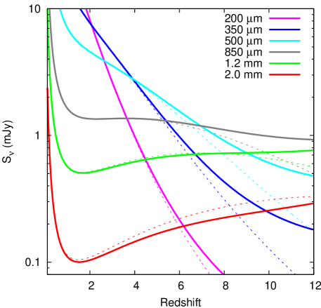
Figure 1.— Redshift-dependent flux density, measured against the CMB, of a galaxy with fixed dust mass $M_{\mbox{d}}=10^{8}M_{\odot}$, dust emissivity index of $\beta$=1.5, i.e. with a FIR luminosity of $L\sim 10^{12}L_{\odot}$, shown for a variety of wavelengths, based on the multi-temperature empirical dust models of Kovács et al. 2010). To radiate the same luminosity against an increasingly warmer CMB in earlier epochs, the cold dust temperature ($T_{0}$=35 K) must rise as $T_{d}^{4+\beta_{\rm eff}}=T_{\rm CMB}^{4+\beta_{\rm eff}}+T_{0}^{4+\beta_{\rm eff}}$ (the effective dust emissivity, $\beta_{\rm eff}$, is defined in Kovács et al. 2010). For comparison, the dashed lines show the same if the CMB heating is ignored. Note, that the observed flux density at 2 mm wavelengths increases monotonically and steeply as a function of redshift for $z>$1.

We have developed the GISMO instrument that utilizes a near background-limited detector to fully exploit the advantages of the 2 millimeter window. Here we report the first deep survey conducted with GISMO centered on the Hubble Deep Field North (HDF-N). The Hubble Deep Field North (HDF-N) is one of the best studied regions in the sky. Its sky coverage is one HST WFPC2 pointing, i.e. $\sim 2.5^{\prime}\times 2.5^{\prime}$, which is less than the $2^{\prime}\times 4^{\prime}$ instantaneous field of view of the GISMO array. The HDF is located in the greater GOODS-N region, which has also been studied in exquisite detail over the last decade at many wavelengths, X-rays: Bra08, UV: 2006AJ....132..853T, Optical: 2004ApJ...600L..93G, optical spectroscopy: 2004AJ....127.3137C, Near-Infrared: 2006NewAR..50..127Y, Mid-Infrared: 2006MNRAS.371.1891R, Far-Infrared:2003MNRAS.344..385B, 2006ApJ...647L...9F, 2008MNRAS.391.1227P, Radio: 2010ApJS..188..178M. In the (sub-)millimeter regime, the HDF and GOODS-N have been studied by the (sub-)millimeter cameras SCUBA, MAMBO, and AzTEC in the past (1998Natur.394..241H, 2005MNRAS.358..149P; 2008MNRAS.389.1489G, 2011MNRAS.410.2749P. The currently available data of the full HDF at 1 mm reach $1-\sigma$ sensitivities of 0.5 mJy/beam (MAMBO observations combined with AzTEC observations, (2011MNRAS.410.2749P), the SCUBA “super”–map (2005MNRAS.358..149P) reaches a peak depth of 0.4 mJy beam${}^{-1}$ at $850~{}\mu$m, however the sensitivity varies significantly over the observed area in the field.

The paper is organized as follows: We first describe the instrument and its characteristics in §2. In §3 we describe observations and the data reduction. In §4 we describe the source extraction and its results, and present simulations used to characterize the data and to evaluate the completeness and reliability of the extracted sources. §5 presents the 2 mm number counts and the analysis of the properties of select individual sources.

2. The GISMO 2 mm Camera

Continuum observations in the 2 mm atmospheric window have not been astronomically explored from the ground to the same degree as has been done at shorter wavelengths (1 mm or less), except for Sunyaev-Zel’dovich (S-Z) observations with dedicated 6 to 10 m class telescopes (2011ApJS..194...41S, 2011PASP..123..568C, 2006NewAR..50..960D). The reason for this is predominantly of technical nature, in particular the very demanding requirements on the noise performance of a background-limited camera operating in this low opacity atmospheric window. In order to provide background-limited observations in the 2 mm window at a good mountain site such as the the IRAM 30 m telescope on Pico Veleta, the required sensitivity, expressed in Noise Equivalent Power (NEP), for the detectors is $\sim 5\times 10^{-17}$ W $\sqrt{\mbox{s}}$ (2006SPIE.6275E..44S), a requirement that is met by our “high” temperature ($T_{c}$ = 450 mK) Transition Edge Sensor (TES) detectors. Consequently we have proposed and built a 2 millimeter wavelength bolometer camera, the Goddard-IRAM Superconducting 2 Millimeter Observer (GISMO, 2008SPIE.7020E...3S) for astronomical observations at the IRAM 30 m telescope on Pico Veleta, Spain (1987A&A...175..319B). GISMO uses a compact optical design (2008SPIE.7020E..66S) and uses an $8\times 16$ array of close-packed, high sensitivity TES bolometers with a pixel size of $2\times 2$ mm${}^{2}$ (2008SPIE.7020E..56B), which was built in the Detector Development Laboratory at NASA/GSFC (2008JLTP..151..266A). The array architecture is based on the Backshort Under Grid (BUG) design (2006SPIE.6275E...9A). GISMO’s bandpass is centered on 150 GHz and has a fractional bandwidth of 20%. The superconducting bolometers are read out by SQUID time domain multiplexers from NIST/Boulder (2002AIPC..605..301I). This design is scalable to kilopixel size arrays for future ground-based, suborbital and space-based X-ray and far-infrared through millimeter cameras (e.g. 2012SPIE.8452E..0TS).

3. Observations & Reduction

The GISMO Deep Field (GDF) observations of the HDF-N were obtained between April 13 and 18, 2011, and on April 11, 12 and 23, 2012. The total integration time was $t\sim 39$ hours, however 2/3 of those observations were obtained with GISMO’s lower sensitivity during the Spring 2011 run (see section 3.4). The FWHM of GISMO’s beam is $17.5"$.

3.1. Data Reduction

The data were reduced, using CRUSH (2008SPIE.7020E..45K), which is the standard reduction software for the GISMO camera. CRUSH is open-source and available in the public domain. The data reduction tool of CRUSH consists of a highly configurable pipeline, which uses a series of statistical estimators in an iterated scheme to separate the astronomical signals from the bright and variable atmospheric background and various correlated instrumental noise signals. It determines proper noise weights for each sample in the time series, removes glitches, identifies bad pixels and other unusable data, and determines the relevant relative gains. It also applies appropriate filters for $1/f$-type noise, and other non-white detector noise profiles. For the detection of point sources, the resulting ”deep”-mode maps are spatially filtered above $50^{\prime\prime}$ FWHM to remove spatially-variant atmospheric residuals. The fluxes in each 10-minute scan are corrected for the line-of-sight atmospheric opacities, based on the IRAM radiometer measurements. Point-source fluxes are also corrected scan-wise for the flux-filtering effect of each and every pipeline step, and for the large-scale structure filtering of the final map. As a result, comparison to point-like calibrator sources (e.g. planets and quasars) is straightforward, even if different reduction options are used for these and the science targets.

3.2. Calibration

Mars, Uranus, and Neptune were observed for primary flux calibration. Of those, measurements of Mars cover the widest range of weather conditions. Using the atmospheric transmission model of the Caltech Submillimeter Observatory and the IRAM 30 m Telescope 225 GHz radiometer readings, we obtain excellent calibration in effectively all weather conditions: a 7% rms blind calibration up to $\tau_{\rm 225GHz}\sim 1$ is obtained. Note that any model uncertainties due to the different elevation of Mauna Kea, the site of the CSO, and Pico Veleta, will be very small and therefore irrelevant for the accuracy of derived calibration factors. Figure 2 shows the histogram of the 2 mm line-of-sight opacities for all data.

Figure 2.— Histogram of the 2-mm line of sight opacities for the GDF observations

3.3. Pointing & Astrometric Accuracy

During the GISMO observing runs in 2011 and 2012, we obtained a large number of pointing measurements over the entire sky, from which we derived appropriate pointing models according to 1996A&AS..115..379G. Our pointing models yield $<$3” rms accuracy in both Az and El directions on all pointing measurements obtained during the two observing runs (424 and 392 individual pointing observations for the 2011 and 2012 observing runs, respectively). Additionally, we frequently checked pointing on nearby quasars during GDF observations. Triggered by a reduction flag, CRUSH will automatically incorporate the measured differential offsets with respect to the pointing model, to further improve pointing accuracy, and to remove most systematic pointing errors in the pointing model, or due to structural deformations of the telescope. The resulting residual pointing errors are expected to be independent and random between independent pointing sessions. Thus, a representative lower bound to the final astrometric accuracy is given by the instantaneous pointing rms ($<$4.2”) divided by the square root of the number of independent pointing sessions spanning the observations. In our case, approximately 30 independent pointing sessions bracket the GDF observations. Therefore, the astrometric accuracy of our map (notwithstanding the inherent positional uncertainties of any detections) could be as low as 0.8” rms, or somewhat higher in the presence of systematics errors, which are not eliminated by the use of nearby pointing measurements.

3.4. Instrument Performance

The noise equivalent flux density (NEFD) of measurements during the 2011 run was typically 15-17 mJy$\sqrt{\mbox{s}}$, under most weather conditions. The obtained sensitivity at that time was mainly limited by a neutral density filter with 40% transmission. This filter was needed, since there was a significant amount of THz light scattered into the GISMO beam by the low pass filters, which were positioned very close to the entrance window of the dewar. In early 2012 we mounted a 77 K baffle dewar in front of the GISMO optical entrance window, which reduces the stray light significantly and eliminates the need for a neutral density filter in the instrument (2012SPIE.8452E..3IS). As a result of this, the NEFD obtained during the 2012 observing run was typically 10 mJy$\sqrt{\mbox{s}}$.

3.5. Noise properties of the beam-smoothed map

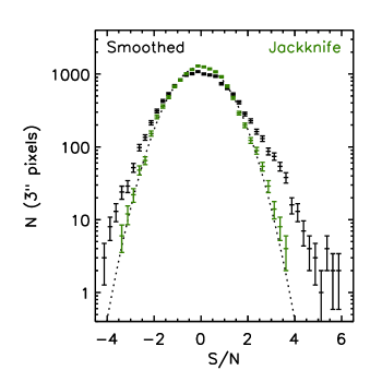
Figure 3.— Signal to noise histogram for the smoothed and filtered GDF data (black), which was used for the source extraction, and shown in Fig. LABEL:GDF, and for a corresponding time-based random jackknife realization (green). The dotted line shows the expected Gaussian noise distribution, based on the radiometric down-integration of the detector timestream noise, with $\sigma=1.00$. The close agreement of the jackknifed noise distribution and the Gaussian expectation indicates that our measurement noise is both closely Gaussian in nature, and radiometric. At the same time, the histogram of the regular (non-jackknifed) map exhibits distinct deviations from the Gaussian noise. A symmetric widening is caused by additional noise from unresolved sources (i.e. confusion noise) on top of the radiometric measurement noise, while resolved emission sources cause the asymmetric excess on the positive half of the distribution.

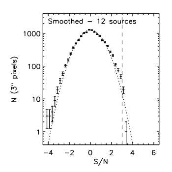
Figure 4.— Signal to noise histogram of the smoothed and filtered GDF data (Fig. LABEL:GDF), after the 12 blindly identified sources are removed and flagged. The vertical dashed line marks the source extraction threshold, resulting in an abrupt truncation of the histogram above the detection threshold. The dotted line shows the expected Gaussian noise distribution from the jackknifed map with $\sigma=1.00$. The post-extraction residuals are more closely Gaussian, as expected, albeit still hinting at the presence of further (fainter) resolved and unresolved sources in the field, which manifest as an asymmetric and a symmetric excess, respectively.

To estimate the noise we randomly multiply each of the individual 10 minute scans by +1 or -1, a method known as “jackknifing”. This eliminates any stationary noise (including sources, and foreground) but retains random noise, including that from the atmosphere. The histogram of the S/N for the jackknifed, beam-smoothed, and filtered GISMO map is shown in Figure 3. The distribution is well fit by a Gaussian with $\sigma=1.00$. The S/N histogram for the regular (not jackknifed) smoothed and filtered map (also Fig. 3) shows distinct excess deviations from the Gaussian distribution on both extremes of the distribution. When we subtract the 12 detected sources (see section 4.3) from the image, the S/N histogram does approach the expected noise distribution as shown in Figure 4. The subtraction of sources (both real and false) causes this histogram to be truncated at the $2.99\sigma$ detection limit. Below this limit both the positive and negative sides of the histogram are more closely Gaussian because the effective smoothed and filtered PSF used for the subtraction has both positive and negative features (main beam and surrounding filter bowl). There is, however, a slight ($\sim 5\%$) symmetric excess remaining in the post-extraction residuals, relative to the jackknifed map. This excess would be consistent with the presence of confusion noise in our map. We cannot, however, quantify the corresponding level of 2-mm confusion noise with any precision because the the noise estimation errors are relatively large given the low number of beams in the field.

4. Source Extraction & Simulations

4.1. Extraction – Method and reliability

The Gaussian nature of noise in our map (section 3.5) is a notable feature of the GISMO data and allows us to provide the strongest possible statistical characterization of our source candidates relying exclusively on formal Gaussian statistics. Because we do not detect any deviation from Gaussian noise, nor see any signs of non-radiometric down-integration in the jackknifed maps, we need not worry about potential troublesome statistical biases that could otherwise result from non-Gaussian, or correlated, noise features.

We extract sources from the beam-smoothed filtered map, which were produced by CRUSH. Beam-smoothing is mathematically equivalent to maximum-likelihood PSF amplitude fitting at every map position (Kovacs-thesis). I.e., the PSF-smoothed map value and its noise directly provide the amplitude and uncertainty of a fitted PSF at each map position. The effective filtered PSF for GISMO maps reduced in ’deep’ mode in CRUSH is accurately modeled as a combination of a 17.5” FWHM Gaussian main beam combined with a negative 50” FWHM Gaussian bowl such that the combined PSF yield zero integral (signifying that we have no DC sensitivity due to the sky-noise removal, and other filtering during the reduction). The 50” FWHM effective PSF bowl is the direct result of explicit large-scale-structure (LSS) filtering during the reduction with a 50” FWHM Gaussian profile. We checked the Gaussian main beam assumption on quasars (detected at high signal-to-noise $>$1000), and confirmed that $>$98% of the integrated flux inside a $R$=50” circular aperture is recovered in the 17.5” FWHM beam-smoothed peak during night-time observations (i.e. for all of our data). We also checked that the filtered PSF accurately recovers the quasar fluxes, when these were LSS filtered the same as our deep field map, and found no further degradation of photometric accuracy associated with the LSS filtering. Therefore, we are very confident that we have sufficient understanding of the effective PSF in our map, and that the systematic errors of the extracted points source fluxes are kept below 2%.

The source extraction code we used is part of the CRUSH software package, and is the same source extraction tool that was used and described in 2009ApJ...707.1201W. It implements an iterated false-detection rate algorithm. Apart from peak position and flux, the algorithm calculates an estimated confidence and an expected cumulative false detection rate for each extracted source. We caution that the confidence levels and false-detection rates are guiding values only, which represent our best statistical estimate without prior knowledge of the 2-mm source counts. A more accurate characterization of confidence levels and/or cumulative false-detection rates would require accurate prior information of the true counts of the 2-mm source population.

4.1.1 Overview of the CRUSH source extraction tool.

Here, we offer a concise summary of the approach implemented by CRUSH ’detect’ tool, which we used for the source extraction.

The expected false detection rate, i.e. the expected number of pure noise peaks mistakenly identified as a source, is given by $N_{f}(\Sigma)=NQ(\Sigma)$, where $N$ is the number of independent Gaussian variables in the map, and $Q(\Sigma)=1-P(\Sigma)$ is the complement cumulative Gaussian probability, i.e. the probability of measuring a deviation larger than a chosen significance, $\Sigma$. A smoothed and filtered map with extraction area $A$ contains

$$N\approx\frac{4.5A}{1.13~{}(\Delta_{\rm smooth}^{2})}\left(1-\frac{\Delta_{\rm smooth}^{2}}{\Delta_{\rm filter}^{2}}\right)$$ (2)

independent variables in terms of the FWHM widths of the Gaussian smoothing ($\Delta_{\rm smooth}$=$\Delta_{\rm beam}$) and the applied large-scale filtering of the map ($\Delta_{\rm filter}$=50”). The right-hand-side term in the formula accounts for the lost degrees of freedom due to the explicit spatial filtering of our map. The approximately 4.5 parameters per smoothing beam were determined empirically based on the occurrence of significant noise peaks in simulated noise maps. The formula was verified to yield close to the expected number of false detections in simulated noise maps with varying areas and filtering properties, and with $N_{f}$ targeted between 0 to 1000. Thus, the above expression will accurately predict the actual false detection rate, as a function of detection threshold, as long as the map noise is known precisely. For our map, with $\sim$321 GISMO beams, a 2.99 $\sigma$ cut yields $N_{f}(2.99)\approx 2$ expected false detections.

Due to the presence of many resolved but undetected sources in the map (asymmetric confusion), our noise estimates are bound to be slightly overestimated (even with the median-noise based estimate used). To our best knowledge, all statistical estimates of map noise, which are based on the observed map itself, will result in overstated noise estimates in the presence of asymmetric confusion (resolved sources below detection). Neither the jackknifed noise, nor radiometric noise, can help offer better estimates, as the extraction noise should include the effect of symmetric confusion (unresolved faint sources) beyond what these can offer. As a result of an inevitably biased noise estimation process, the corresponding false detection rate estimates are slightly above actual, and represent a useful conservative upper bound. This is confirmed by the simulations, presented in section LABEL:sec:sims, which found that if the 2 mm source counts were those of, e.g., 2011A&A...529A...4B or 2011ApJ...742...24L, then the actual false detection rate would be 1.34 or 0.55, respectively, vs. the expected 2. However, as we stated earlier, we cannot unbias our noise estimates, or quantify the true false detection rate, without prior knowledge of the true 2-mm source counts, which are not well-constrained at present. Instead, our estimates offer strong upper bounds for the unknown actual false-detection rates.

Each source identified above the significance cut is removed from the map with the smoothed and filtered point-spread function before the extraction proceeds. Subtraction with the filtered PSF allows the detection of further nearby peaks, which may have been previously suppressed by the negative filter bowl surrounding the previous detections. The circular area ($r^{2}$=$\Delta_{\rm beam}^{2}+\Delta_{\rm smooth}^{2}$) containing the main beam of the detected source is flagged after the extraction, since it no longer contains meaningful information after the removal of the source from within. To ensure that our catalog is based on the most accurate measure of the map noise and zero levels, CRUSH estimates the zero level using the mode of the map flux distribution, and estimates the noise from the median observed deviation median$(x^{2})\approx 0.454937\sigma^{2}$). Both measures are relatively robust and reasonably unbiased by the presence of relatively bright sources, or localized features, in the map.

For each source candidate, CRUSH estimates a detection confidence based on the expected false detection rate $N_{f}$. According to Poisson statistics, the detection confidence $C$ of a single peak is the probability that no such peak occurs randomly, i.e. $P_{0}(N_{f})=e^{-N_{f}}$. This is then further refined to include information from other sources already detected in the map. Thus, if $n$ true sources with apparent significance above $\Sigma$ are known a priori to exist in the map, than any given peak at significance $\Sigma$ may be one of $n$ sources, or one of the $N_{f}$ expected false detections, hence the probability of false detection for each of $n+N_{f}$ peaks is reduced by a factor of $N_{f}/(n+N_{f})$. (In other words, we should expect only $N_{f}$ false detections (noise peaks) for every $n$ actual sources detectable above a given threshold.) CRUSH uses the number of sources $N(>\Sigma)$ that were already extracted above significance $\Sigma$ minus the expected false detection rate $N_{f}(\Sigma)$ as a self-consistent proxy for $n$, which is a reasonable assumption when prior knowledge of the actual underlying counts is not readily available (as in our case). As such, the individual confidence levels of consecutive detections are estimated as

$$C(\Sigma)=1-\frac{N_{f}(\Sigma)}{N(>\Sigma)}\left(1-e^{-N_{f}(\Sigma)}\right).$$ (3)

4.2. Deboosting

Deboosting is a statistical correction to the observed flux densities, when source counts fall steeply with increasing brightness (e.g. 2010ApJ...718..513C and references therein). Thus, in a statistical ensemble of sources, the same observed flux arises more often from one of many fainter sources than from the few brighter ones, relative to the measured value. We assume a measurement with Gaussian noise (validated by the closely Gaussian jackknife noise distribution) and a 2 mm source count model scaled from observationally constrained 850$\mu$m counts (e.g. 2006MNRAS.372.1621C, 2009ApJ...707.1201W) assuming $T_{d}/(1+z)\gtrsim$ 10 K (2006ApJ...650..592K) and dust emissivity index ($\beta$) of 1.5 (2010ApJ...717...29K). We also deboosted our data using the physical number-count models of 2011ApJ...742...24L and 2011A&A...529A...4B, see section LABEL:sec:counts.

For deboosting we followed a Bayesian recipe, such as described in 2005MNRAS.357.1022C; 2006MNRAS.372.1621C:

$$p(S_{i}|S_{o},\sigma)\propto p(S_{i})~{}p(S_{o},\sigma|S_{i})$$ (4)

expressing the probability of intrinsic source flux $S_{i}$ in terms of the observed flux $S_{o}$ and its measurement uncertainty $\sigma$.

However, we made some important modifications to the recipe to account for the possibility that the observed flux arises from multiple overlapping galaxies, and we account for confusion. Accordingly, we replace the single isolated source assumption $p(S_{i})\propto\frac{dN}{dS}(S_{i})$ of 2005MNRAS.357.1022C; 2006MNRAS.372.1621C, with the compound probability that one or more (up to $m$) resolved sources in the beam contribute to an aggregated intrinsic flux $S_{i}$:

$$p(S_{i})=\int_{0}^{S_{i}}dS_{1}~{}...\int_{0}^{S_{m-1}}dS_{m}~{}\pi(S_{1})~{}...~{}\pi(S_{m})~{}\delta\left(S_{i}-\sum_{k=1}^{m}S_{k}\right).$$ (5)

Inside the integrals is the product of the individual component probability densities $\pi(S_{k})$, which correspond to $S_{i}$ arising from a specific combination of ($S_{1}~{}...~{}S_{m}$) individual components. The delta function ensures that the component fluxes considered add up to the total intrinsic flux $S_{i}$ when integrated. Each nested integral for $S(k)$ is performed up to the previous flux $S_{k-1}$, indicating that each successive component $S_{k}$ is no brighter than the previous one $S_{k-1}$, and ensuring that each particular combination of fluxes is counted one time only. Once the fluxes in the outer integrals sum up to $S_{i}$, the remaining inner integrals can be skipped (in numerical implementations) corresponding to fewer than $m$ actual contributors (or to keep to a more formal notation we can add the delta function at zero, i.e. $\delta(S_{k})$, to the definition of $\pi(S_{k})$ below to achieve exactly without omitting the any inner integrals). When overlaps are ignored ($m$=1), Eq. 5 reduces to $p(S_{i})=\pi(S_{i})$ naturally (no integration required).

The differential source counts $\frac{dN}{dS}(S_{k})$ determine the probability that there is at least one intrinsic source with brightness $S_{k}$ in the beam, resolved or unresolved. The distinction between resolved and unresolved sources is important: unresolved sources cause a symmetric widening of the map noise distribution (confusion noise) compared to the experimental noise (e.g. radiometric down-integration as measured by a jackknife); resolved sources, on the other hand, detected or not, will manifest as an excess of flux on the positive side of the observed flux (or S/N) distribution. Deboosting naturally needs to consider resolved sources only.

If one distributes $N$ sources randomly in some large area $A$ (for simplicity’s sake let’s consider the same area to which the counts are normalized, whether deg${}^{2}$ or sr) with $N_{b}=A/2\pi\sigma_{b}^{2}$ ($N_{b}$$\gg$1) independent beams (FWHM$\approx$2.35 $\sigma_{b}$), then the chance that none of these sources fall into a given beam (our detection beam) is:

$$q(N)=\left(1-\frac{1}{N_{b}}\right)^{N}\approx e^{-N/N_{b}}$$ (6)

Therefore, at a given flux density $S_{k}$ the probability density of a source with brightness $S_{k}$ being resolved (i.e. unblended with brighter ones) is

$$\pi_{+}(S_{k})\approx\frac{1}{N_{b}}~{}\frac{dN}{dS}(S_{k})~{}e^{-N(>S_{k})/N_{b}},$$ (7)

in terms of the integrated number counts $N$($>$$S$), and the corresponding differential counts $\frac{dN}{dS}$. Here, $\pi_{+}(S_{k})$ measures the probability density that at least one resolved source with flux $S_{k}$ falls inside the detection beam, and does not exclude the possibility of further fainter components within the same beam (hence the plus sign as the subscript). Using $\pi_{+}(S_{k})$, however, we can easily express the probability density $\pi(S_{k})$ for exactly one component with $S_{k}$ in a given beam, by simply subtracting the integrated probability that there is at least one other fainter object in that same beam with the first one:

$$\pi(S_{k})=\pi_{+}(S_{k})\left(1-\int_{0}^{S_{k}}\pi_{+}(S)~{}dS\right).$$ (8)

For the highest order $m$ under consideration, we may truncate by setting $\pi(S_{m})\approx\pi_{+}(S_{m})$. The approximation is valid as long as $m$ is chosen to be large enough such that resolved overlaps with further components (the right-hand integral term) are negligible.

For the particular case of the GISMO 2 mm sources, we considered up to 3 overlapping components ($m$=3) contributing to the observed fluxes. We verified that this was sufficient, as we noticed no measurable degree of incremental change in the deboosted values (and profiles) between $m$=2 and $m$=3. We chose $m$=3 to be on the safe side. At the same time allowing for at least 2 overlapping components instead of just a single isolated source ($m$=1) did have a significant impact on the deboosting results, justifying our modified approach.

Since our source extraction algorithm determines the map zero level as the mode (not the mean) of the distribution, the extracted source fluxes are easily measured against the unresolved background. And, because our deboosting method is based on resolved sources only, it also means that no additional zero-level adjustment is necessary. As a result, the distribution naturally does not extend to negative fluxes, as is demonstrated by the posterior probability distributions of the extracted GISMO sources shown in the appendix.

4.3. Extraction – Results

Table 1GDF 2mm Sources

ID	RA	DEC	$S$	S/N	confidence	$N_{f}$
	[J2000]	[J2000]	[mJy]		[%]
GDF-2000.1	12:36:33.98	62:14:08.0	0.79$\pm$0.14	5.53	100	0.000
GDF-2000.2	12:37:05.95	62:11:47.2	0.67$\pm$0.16	4.18	99	0.021
GDF-2000.3	12:37:12.17	62:13:20.4	0.78$\pm$0.19	4.10	99	0.029
GDF-2000.4	12:36:29.54	62:13:11.7	0.53$\pm$0.15	3.51	87	0.330
GDF-2000.5	12:36:51.40	62:15:39.1	0.61$\pm$0.18	3.37	87	0.541
GDF-2000.6	12:36:52.06	62:12:26.4	0.42$\pm$0.13	3.33	89	0.627
GDF-2000.7	12:36:57.09	62:13:29.7	0.40$\pm$0.12	3.24	89	0.875
GDF-2000.8	12:37:10.12	62:13:35.5	0.54$\pm$0.17	3.22	89	0.918
GDF-2000.9	12:36:36.54	62:11:13.5	0.51$\pm$0.16	3.17	84	1.117
GDF-2000.10	12:36:25.16	62:14:10.5	0.87$\pm$0.29	3.06	84	1.630
GDF-2000.11	12:36:45.88	62:14:42.2	0.43$\pm$0.14	3.04	84	1.735
GDF-2000.12	12:36:56.17	62:10:19.1	0.54$\pm$0.19	3.02	84	1.828

Note. — $N_{f}$ is the expected cumulative false detection rate as defined in Section 4.1. The maps are beam-smoothed (by 17.5” FWHM) to an effective $24.7^{\prime\prime}$ FWHM image resolution for point source extraction

Table 2Deboosted 2mm Flux Densities Assuming Different Source Counts or Models

ID	deboosted $S^{\prime}$ [mJy]
	Lapi et al.	Coppin et al.	Bethermin et al.
GDF-2000.1	0.75 $\pm$ 0.16	0.69 $\pm$ 0.14	0.71 $\pm$ 0.16
GDF-2000.2	0.56 $\pm$ 0.21	0.53 $\pm$ 0.18	0.51 $\pm$ 0.20
GDF-2000.3	0.63 $\pm$ 0.25	0.59 $\pm$ 0.22	0.56 $\pm$ 0.25
GDF-2000.4	0.39 $\pm$ 0.20	0.37 $\pm$ 0.18	0.35 $\pm$ 0.19
GDF-2000.5	0.40 $\pm$ 0.24	0.38 $\pm$ 0.21	0.34 $\pm$ 0.23
GDF-2000.6	0.31 $\pm$ 0.16	0.29 $\pm$ 0.15	0.28 $\pm$ 0.16
GDF-2000.7	0.29 $\pm$ 0.15	0.27 $\pm$ 0.14	0.26 $\pm$ 0.15
GDF-2000.8	0.35 $\pm$ 0.22	0.33 $\pm$ 0.20	0.30 $\pm$ 0.20
GDF-2000.9	0.33 $\pm$ 0.20	0.31 $\pm$ 0.19	0.28 $\pm$ 0.19
GDF-2000.10	0.40 $\pm$ 0.33	0.37 $\pm$ 0.30	0.30 $\pm$ 0.29
GDF-2000.11	0.28 $\pm$ 0.17	0.26 $\pm$ 0.16	0.25 $\pm$ 0.17
GDF-2000.12	0.33 $\pm$ 0.23	0.31 $\pm$ 0.21	0.24 $\pm$ 0.20

Note. — Derived by extrapolation of the 2006MNRAS.372.1621C SHADES number counts to 2 mm counts, or from the 2011ApJ...742...24L or 2011A&A...529A...4B models.

Table 3GDF 2 mm Sources with (sub-)mm counterparts

ID	$z$	ID	$S$($850\mu$m)	$S^{\prime}$($850\mu$m)	ID	$S$(1.2 mm)	$S^{\prime}$(1.2 mm)	$\delta r$
			[mJy]	[mJy]		[mJy]	[mJy]	[${}^{\prime\prime}$]
GDF-2000.1	4.042	GN 850.10	11.3$\pm$1.6	8.6$\pm$4.8	AzGN03	5.2$\pm$0.6	4.7$\pm$1.7	6.0
GDF-2000.3	1.992	GN 850.39	7.4$\pm$2.0	3.8$\pm$2.8	AzGN07A${}^{*}$	blend${}^{*}$	$\cdots$	9.8
					GN1200.3	3.9$\pm$0.6	3.3$\pm$1.3
GDF-2000.6	5.183	GN 850.14	5.9$\pm$0.3	5.9$\pm$0.3	AzGN14	2.9$\pm$0.6	2.2$\pm$1.0	1.6
GDF-2000.8	1.97		$<6$	$\cdots$	AzGN07B${}^{*}$	blend${}^{*}$	$\cdots$	13.8
GDF-2000.11	2.30	GN 850.12	8.6$\pm$1.4	6.4$\pm$3.6	AzGN08	3.0$\pm$0.6	2.4$\pm$1.1	6.6

Note. — MAMBO/AzTEC 1.2 mm data are from 2008MNRAS.389.1489G and 2008MNRAS.391.1227P, SCUBA $850\mu$m data from 2003MNRAS.344..385B, 2005MNRAS.358..149P, and 2008MNRAS.389.1489G. $z$ is the measured redshift. The deboosted flux values $S^{\prime}$ are based on the SHADES counts, using the same equations used for calculating the 2 mm data counts in order to be consistent with the deboosting of the 2 mm fluxes shown in Table 2.

${}^{*}$ Both, GDF-2000.3 and GDF-2000.8, are associated with AzGN07, which implies that this 1.2 mm source is a blend of two sources.

Table 4low S/N GDF 2mm Sources – identified through (sub-)mm counterparts

ID	RA	DEC	$S$(2mm)	$z$	ID	$\lambda$	$S$	$S^{\prime}$	$\delta r$
	[J2000]	[J2000]	[mJy]				[mJy]	[mJy]	[${}^{\prime\prime}$]
GDF-2000.13	12:37:12.01	62:12:14.0	0.52$\pm$0.20	2.91	GN 850.21	850 $\mu$m	5.7$\pm$1.2	3.8$\pm$2.3	8.1
				2.91	GN 1200.29	1200 mm	2.6$\pm$0.6	1.9$\pm$0.9	0.0
GDF-2000.14	12:36:27.40	62:12:13.8	0.50$\pm$0.19	4.69	AzGN10	1200 mm	2.6$\pm$0.6	1.9$\pm$0.9	4.9
GDF-2000.15	12:36:45.00	62:11:47.1	0.36$\pm$0.15	$\cdots$	GN 850.28	850 $\mu$m	1.7$\pm$0.4	0.6$\pm$0.6	1.8

Note. — $z$ is the measured redshift. Deboosted flux values $S^{\prime}$ were calculated directly (850$\mu$m) from or extrapolated (1.2 mm) from the SHADES number counts.

Table 5Deboosted 2mm Flux Densities Assuming Different Source Counts or Models

ID	deboosted $S^{\prime}$ [mJy]
	Coppin et al.	Lapi et al.	Bethermin et al.
GDF-2000.13	0.26 $\pm$ 0.21	0.24 $\pm$ 0.20	0.21 $\pm$ 0.19
GDF-2000.14	0.25 $\pm$ 0.20	0.23 $\pm$ 0.19	0.20 $\pm$ 0.18
GDF-2000.15	0.21 $\pm$ 0.15	0.17 $\pm$ 0.14	0.17 $\pm$ 0.14

Note. — Derived by extrapolation of the 2006MNRAS.372.1621C SHADES number counts to 2 mm counts, and from the 2011ApJ...742...24L or 2011A&A...529A...4B models.

Table 6GDF 2mm Sources – derived parameters

ID	$|\hat{\chi}^{2}|$	$T_{c}$	$\log M_{d}$	$\log L$	$q_{L}$	$q_{IR}$	$\tau_{\rm peak}$
		[K]	[$M_{\odot}$]	[$L_{\odot}$]
GDF 2000.1	0.70	51.2 $\pm$ 2.0	8.53 $\pm$ 0.07	13.52 $\pm$ 0.06	2.83$\pm$0.21	3.08 $\pm$ 0.21	1.28
GDF 2000.3	1.08	40.8 $\pm$ 0.7	8.59 $\pm$ 0.14	13.10 $\pm$ 0.03	2.68 $\pm$ 0.10	2.91 $\pm$ 0.10	1.08

Note. — All quantities were fitted using the measured redshifts (Table 2), temperature-distribution model ($dM_{d}/dT\propto T^{-7.2}$) with $\beta=1.5$ and assuming a 2 kpc emission diameter. The dust masses assume $\kappa(850\mu$m)=0.15 m${}^{2}$ kg${}^{-1}$. Uncertainties are 1 $\sigma$ total errors of the fits to data, which do not include the uncertainties in the redshift values. The following quantities are shown in the table: $|\hat{\chi}^{2}|$ residual scatter around the fit, $T_{c}$ temperature of the dominant cold component, $M_{d}$ dust mass, $L$ integrated IR luminosity, $q_{L}$ radio–(F)IR correlation constant as defined in 2010ApJ...717...29K, $q_{\rm IR}$ radio–(F)IR correlation constant as defined in 2010MNRAS.402..245I, and $\tau_{\rm peak}$ optical depth around the IR emission peak.