Non perturbative effects of primordial curvature perturbations on the apparent value of a cosmological constant

Abstract

We study effects on the luminosity distance of a local inhomogeneity seeded by primordial curvature perturbations of the type predicted by the inflationary scenario and constrained by the cosmic microwave background radiation. We find that a local underdensity originated from a one, two or three standard deviations peaks of the primordial curvature perturbations field can induce corrections to the value of a cosmological constant of the order of $0.6\%,1\%,1.5\%$ respectively. These effects cannot be neglected in the precision cosmology era in which we are entering. Our results can be considered an upper bound for the effect of the monopole component of the local non linear structure which can arise from primordial curvature perturbations and requires a fully non perturbative relativistic treatment.

I Introduction

Before the invention of the inflationary scenario of the early Universe, the standard cosmological model was based on the assumption of global large scale homogeneity and isotropy (often dubbed ”the Cosmological principle”) which reflects itself in the observed approximate isotropy of the Hubble flow and the temperature of the cosmic microwave background (CMB) radiation. With the inflationary scenario, there is no more need in such assumption since viable realizations of this scenario predict the large-scale space-time metric to be approximately homogeneous and isotropic up to very large (but still finite) scales fantastically exceeding the present Hubble radius. In addition, these viable inflationary models predict a specific structure of small inhomogeneous metric perturbations of the scalar and tensor types inside the observed part of Universe (inside the last scattering surface if speaking about photons). These perturbations are supposed to be the seeds of the CMB angular temperature anisotropy and polarization. Also, from the scalar perturbations, galaxies and their clusters, as well as other compact objects and the large-scale structure of the spatial distribution of galaxies in the Universe, have been formed at later time due to gravitational instability. Due to the quantum (in fact, quantum-gravitational) origin of these small primordial perturbations in the inflationary scenario, they can be very well described as classical stochastic quantities with the almost Gaussian statistics. Because of this stochasticity, the Cosmological principle is not exact even at observable scales less than the Hubble radius, some deviations from it are certainly expected, though of a specific type and sufficiently small probability, e.g. near large extrema of perturbations. However, cosmic variance Marra:2013rba ; Li:2008yj ; Shi:1997aa ; Wang:1997tp ; 2013A&A ; Ben-Dayan:2014swa makes such a possibility viable and worth investigation. It should be emphasized that the effects we study in this letter correspond to highly non linear structures which cannot be studied using a perturbative approach, since the relativistic correction can be dominant Bolejko:2012uj , and for this reason they can differ from previous estimations of the effects of cosmic variance which were based on perturbative relativistic or Newtonian approximations.

That is why we study the effects of late time local inhomogeneities corresponding to large peaks of the primordial scalar (curvature) perturbations on the apparent values of parameters of the standard cosmological model, mainly on the value of a cosmological constant. We model a present day local inhomogeneity around such a large peak by the Lemaitre-Tolman-Bondi (LTB) solution with the initial condition compatible with inflation, i.e. with the homogeneous initial curvature singularity. The spherical symmetry of the metric is justified by the known property of large peaks of a Gaussian random field Bardeen:1985tr to be approximately spherically symmetric, and we consider the case in which an observer is located at the center of the peak. In this way we are able to relate the local inhomogeneity to the primordial curvature perturbation spectrum constrained by CMB anisotropy observations. Previous studies have shown how ignoring the presence of such a local inhomogeneity could lead to the wrong conclusion of the presence of evolving dark energy Romano:2010nc , while in fact dark energy is simply a cosmological constant. Similar approach was used in Valkenburg:2011ty and Marra:2012pj . Here we consider the effects on the supernovae Ia luminosity distance, and quantify the effect on the estimation of the apparent value of the cosmological constant. Other attempts to study the effects of inhomogeneities on cosmological observables consisted in implementing some averaging procedure Romano:2006yc ; Romano:2009xw ; Fanizza:2013doa ; BenDayan:2013gc ; Buchert:2001sa ; Buchert:2002ht or to consider inhomogeneities as alternative to dark energy GarciaBellido:2008yq ; February:2009pv ; Uzan:2008qp ; Clarkson:2007bc ; Zuntz:2011yb ; Ishibashi:2005sj ; Bolejko:2011ys ; Romano:2009xw ; Romano:2007zz ; Romano:2012yq ; Romano:2009qx ; Zibin:2011ma ; Bull:2011wi ; Balcerzak:2012bv .

Following the definition of apparent value of the cosmological constant given in Romano:2011mx we find that the effects of a local overdensity are not very important, while a local underdensity can lead to a correction of the apparent value of the cosmological constant up to a order of $1.5\%$, which cannot be ignored in high precision cosmology. While our approach here is based on making a theoretical connection between the local Universe today and early Universe physics, there have been some recent direct observational evidences Keenan:2013mfa which we may actually live inside a local inhomogeneity, which could have arisen from a primordial curvature perturbation peak of the type we study here, as predicted by Bardeen:1985tr . Other possible evidences of being located inside a local inhomogeneity come from the apparent tension between the estimation of cosmological parameters from local observations and the Planck satellite results Verde:2013wza ; Ade:2013zuv .

II Primordial curvature perturbations and late time inhomogeneities

The metric after inflation on scales much larger than the Hubble scale can be written as

$$ds^{2}=-dt^{2}+a_{F}^{2}(t)e^{2\zeta({\bf r})}(dr^{2}+r^{2}d\Omega^{2})\,$$ (1)

where $r=|{\bf r}|$, and $\zeta({\bf r})$ may be interpreted as a local, space-dependent number of $e$-folds $N$ from a hypersurface of uniform spatial scalar curvature (called the flat hypersurface) during inflation (up to a constant absorbable into $a_{F}$). This relation is the basis of the so-called $\delta N$ formalism, first used in Starobinsky:1982ee in the case of a single field inflation, and then extended to multiple field inflation in Starobinsky:1986fxa ; Sasaki:1995aw . Here we neglect tensor perturbations (primordial gravitational waves) since, first, their power is suppressed by at least one order of the small inflationary slow-roll parameter $\varepsilon$ compared to scalar (curvature) perturbations and, second, they are not subjected to gravitational instability and their amplitude decreases $\propto a_{F}^{-1}$ inside the Hubble radius. Near large peaks of primordial perturbations, we approximate $\zeta=\zeta(r)$. Such points certainly exist somewhere in space.

The Lemaitre-Tolman-Bondi (LTB) solution is a pressureless spherically symmetric solution of Einstein’s field equations given by Lemaitre:1933qe ; Tolman:1934za ; Bondi:1947av

$$ds^{2}=-dt^{2}+\frac{\left(R,_{r}\right)^{2}dr^{2}}{1+2\,E(r)}+R^{2}d\Omega^{2}\,,$$ (2)

where $R$ is a function of the time coordinate $t$ and the radial coordinate $r$, $E(r)$ is an arbitrary function of $r$, and $R_{,r}=\partial_{r}R(t,r)$. The Einstein’s equations with a cosmological constant give

$$\left({\frac{\dot{R}}{R}}\right)^{2} = \frac{2E(r)}{R^{2}}+\frac{2M(r)}{R^{3}}+\frac{\Lambda}{3}\,,$$ (3)

$$\rho(t,r) = \frac{2M,_{r}}{R^{2}R,_{r}}\,,$$ (4)

where $M(r)$ is an arbitrary function of $r$, $\dot{R}=\partial_{t}R(t,r)$ and $c=8\pi G=1$ and is assumed in the rest of the paper. We will also adopt, without loss of generality, the coordinate system in which $M(r)\propto r^{3}$, and fix the geometry of the solution by using a function $k(r)$ according to $2E(r)=-k(r)r^{2}$.

As shown in Romano:2010nc it is possible to choose an appropriate time when we can match the LTB metric and the metric after inflation given in eq.(1). The result is a relation between the primordial curvature perturbation and the function $k(r)$ :

$$k(r)=-\frac{1}{r^{2}}[(1+r\zeta^{\prime})^{2}-1]\,,$$ (5)

which in the linear regime $r\zeta^{\prime}\ll 1$ reduces to

$$k(r)=-2\frac{\zeta^{\prime}(r)}{r}\,.$$ (6)

The approximation of the spherical symmetry is justified by the known property of a Gaussian random field Bardeen:1985tr according to which large peaks of a stochastic function tend to have a spherical shape. In the rest of the paper we will make the additional assumption to be located at the center of such a spherically symmetric inhomogeneity. This is supported by other evidences of isotropy such as the cosmic microwave background (CMB) radiation, implying that if any local inhomogeneity around us is actually present, this should be highly spherically symmetric. In this sense the effects we will consider are associated to the monopole component of the local structure surrounding us, assuming this was seeded by a few $\sigma$ peak of the metric perturbation $\zeta$. Such perturbation still corresponds to a small additional density contrast if its size is sufficiently large. The assumption of being located at the center of such a peak allows us to set an upper bound on the magnitude of the effects on the estimation of cosmological parameters, in particular on the value of the cosmological constant.

Figure 1: In the top $k(r)$ is plotted for $A=2\times(5\times 10^{-5})$ (top) and $A=-2\times(5\times 10^{-5})$ (bottom), and $\zeta(r)$ in the bottom for $A=2\times(5\times 10^{-5})$ (top) and $A=-2\times(5\times 10^{-5})$ (bottom). Different lines correspond to different values of $\sigma$, expressed in units of $H_{0}^{-1}$.

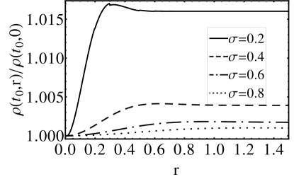
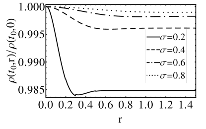
Figure 2: The energy density ratio $\rho(t_{0},r)/\rho(t_{0},0)$ at the time observation $t_{0}$ is plotted as function of the radial coordinate for $A=-2\times(5\times 10^{-5})$ on the left and $A=2\times(5\times 10^{-5})$ on the right. As can be seen positive primordial curvature perturbations, correspond to a central overdensity, and negative primordial curvature perturbations correspond to a central underdensity. Another important feature is that larger values of $\sigma$ correspond to smaller levels of inhomogeneity. The radial coordinate $r$ and $\sigma$ are expressed in units of $H_{0}^{-1}$.

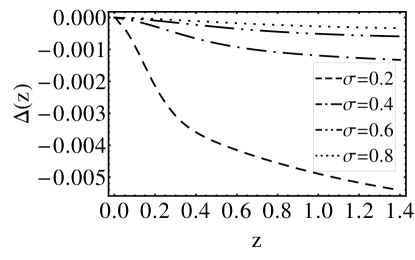
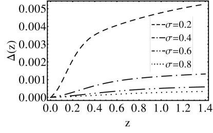
Figure 3: The relative difference $\Delta(z)=(D_{L}^{\Lambda CDM}(z)-D_{L}^{\Lambda LTB}(z))/D_{L}^{\Lambda CDM}(z)$ of the luminosity distance between the $\Lambda LTB$ case and $\Lambda CDM$ is plotted for different values of $\sigma$, where the latter is in units of $H_{0}^{-1}$. The left figure corresponds to $A=-2\times(5\times 10^{-5})$ and the right to $A=2\times(5\times 10^{-5})$. A local underdensity, corresponding to $A<0$, is associated to a larger luminosity distance respect to the homogeneous case, while local overdensities give a smaller distance. $\sigma$ is expressed in units of $H_{0}^{-1}$.

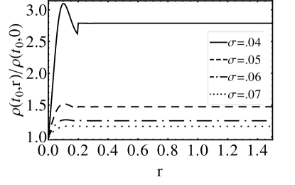
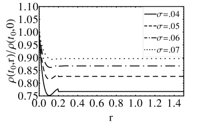
Figure 4: The energy density ratio $\rho(t_{0},r)/\rho(t_{0},0)$ at the time observation $t_{0}$ is plotted as function of the radial coordinate for $A=-2\times(5\times 10^{-5})$ on the left and $A=2\times(5\times 10^{-5})$ on the right. As can be seen small values of $\sigma$ correspond to very large levels of inhomogeneity, making them incompatible with observations. The radial coordinate $r$ and $\sigma$ are expressed in units of $H_{0}^{-1}$.

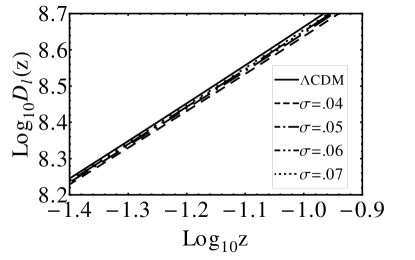
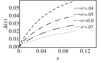
Figure 5: On the top the luminosity distance is plotted for different values of $\sigma$ in units of $H_{0}^{-1}$. On the bottom the relative difference $\Delta(z)=(D_{L}^{\Lambda CDM}(z)-D_{L}^{\Lambda LTB}(z))/D_{L}^{\Lambda CDM}(z)$ of the luminosity distance between the LTB case and $\Lambda CDM$ is plotted for different values of $\sigma$, in units of $H_{0}^{-1}$. The left figures corresponds to $A=-2\times(5\times 10^{-5})$ and the right to $A=2\times(5\times 10^{-5})$. These figures correspond to small values of $\sigma$, showing how the corresponding effective $H_{0}$ for $\sigma<0.04$, estimated as a low redshift slope of the luminosity distance, is not compatible with the observed value.

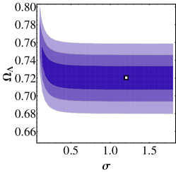
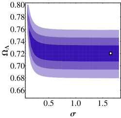
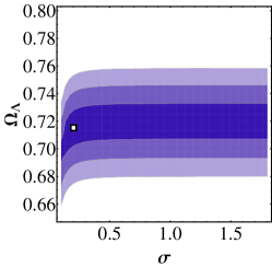
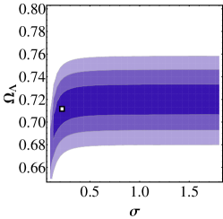
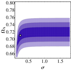
Figure 6: The contour plots for the luminosity distance $\chi^{2}$ are shown for the parameters $\Omega_{\Lambda}$ and $\sigma$, expressed in units of $H_{0}^{-1}$. For the top figures $A=1\times 5\times 10^{-5}$ , $A=2\times 5\times 10^{-5}$ and $A=3\times 5\times 10^{-5}$, from left to right respectively. For the bottom figures $A=-1\times 5\times 10^{-5}$, $A=-2\times 5\times 10^{-5}$ and $A=-3\times 5\times 10^{-5}$, from left to right respectively.

III Effects on the estimation of the apparent value of the cosmological constant from supernova Ia luminosity distance

Our goal is to assess what could be the effect on the estimation of the value of the cosmological constant due to a local inhomogeneity seeded by a fluctuation of the primordial curvature perturbation. In particular we will focus on the effects on the supernovae Ia luminosity distance observations. In our analysis we will use the Union $2.1$ compilation data set Suzuki:2011hu .

Given the assumption of the central location of the observer, we need to solve the radial null geodesics Celerier:1999hp

$${dr\over dz} = {\sqrt{1+2E(r(z))}\over{(1+z)\dot{R^{\prime}}[T(r(z)),r(z)]}}\,,$$ (7)

$${dt\over dz} = -\,{R^{\prime}[T(r(z),r(z))]\over{(1+z)\dot{R^{\prime}}[T(r(z)),r(z)]}}\,,$$ (8)

and then substitute in the formula for the luminosity distance in a LTB space

$$D_{L}(z) = (1+z)^{2}R(t(z),r(z))\,.$$ (10)

We will model the primordial curvature perturbations with a Gaussian profile:

$$\zeta(r)=Ae^{-(\frac{r}{\sigma})^{2}}\,,$$ (11)

and fit data with the corresponding LTB solution given by eq.(5). The initial conditions for the geodesic equations are obtained from the Einstein’s equations at the center, and the age of the Universe used as initial condition for the time geodesics and reported in the last column of Table I is obtained by integrating with respect to the scale factor from the big-bang till today. The parameter $\sigma$ is associated to the scale of the inhomogeneity, while $A$ is related to its amplitude. From observational constraints from the CMB anisotropy spectrum we know that the standard deviation of the primordial curvature perturbation $\zeta(r)$ should be about $5\times 10^{-5}$, so we will consider peaks with $A$ equal to some multiples of this value. The relation between $k(r)$ and $\zeta(r)$ is shown in Fig. 1, for different values of $A$ and $\sigma$. The present density contrast corresponding to peaks of the primordial curvature perturbations with different values of $A$ and $\sigma$ is shown in Fig. 2, while the effects on the luminosity distance are shown in Fig. 3.As can be seen small values of $\sigma$ are associated to larger $k(r)$, which also correspond to greater observational effects. For this reason very small values of $\sigma$ are observationally excluded, since they would correspond to very high density contrasts today, and they would also be incompatible with local measurements of the Hubble parameter as shown in Fig. 5-4. The results of the data fitting are shown in the contour plots for the parameters ${\sigma,\Omega_{\Lambda}}$ in Fig. 6. As can be seen in Fig. 2 positive values of $A$ correspond to central overdensity, and negative values to underdensities. The effects on the luminosity distance are shown for both positive and negative curvature perturbations peaks in Fig 3. For negative peaks we have an increase of the luminosity distance with respect to a $\Lambda CDM$ with the same value of $\Omega_{\Lambda}$, while for positive peaks the effect is the opposite.

As it can be seen from the luminosity distance plots, values of $\sigma$ lower than 0.1 introduce a large effect on the value of $H_{0}$, making this area of the parameter space incompatible with observational data of the Hubble parameter, but this does not affect our conclusions, since we find that the best fit parameters correspond to $\sigma>0.2$.

$A/(5\times 10^{-5})$	$\sigma$	$\Omega_{\Lambda}$	$\chi^{2}_{min}$	$t_{0}$
3	1.64	0.7204	562.242	0.983023
2	1.212	0.7204	562.242	0.982992
1	0.864	0.7204	562.242	0.982995
0		0.72	562.242	0.982778
-1	0.209	0.7155	562.217	0.981357
-2	0.228	0.7124	562.202	0.980357
-3	0.232	0.709	562.190	0.979288

Table 1: The table shows the values of $\sigma$, expressed in units of $H_{0}^{-1}$, and $\Omega_{\Lambda}$ minimizing the $\chi^{2}$ for different values of the amplitude A, where the latter is expressed in integer multiples of the $5\times 10^{-5}$, the value of the standard deviation of the primordial curvature perturbations implied by CMB observations. Positive values of A do not improve appreciably the value of $\chi^{2}$, neither affect greatly the best fit values for $\Omega_{\Lambda}$, while negative values improve the $\chi^{2}$ and also affect considerably the best fit value for $\Omega_{\Lambda}$. The row corresponding to $A=0$ gives the best fit values for a flat $\Lambda CDM$ model, and is reported as a reference for the magnitude of the effects of the local inhomogeneity. The last column corresponds to the age of the Universe in units of $H_{0}^{-1}$, showing how the effect on this is smaller than on the cosmological constant.

From the table I we can see that the effects on the estimation of the value of the cosmological constant can be of the order of $\approx 1.5\%$, which cannot be ignored, since they are of the order of magnitude of other sources of systematic errors.

IV Conclusions

We have studied the effects of late time inhomogeneities seeded by primordial curvature perturbations on the luminosity distance of supernovae Ia, and consequently on the estimation of the apparent value of a cosmological constant. Our analysis shows that these effects cannot be ignored in the high precision cosmology era in which we are entering and should be properly taken into account. Fitting data under the a priori assumption of exact background homogeneity could overestimate the value of the cosmological constant by up to $1.5\%$. The same kind of conclusions can apply to other cosmological parameters whose estimation can be affected by local structure and suggests the importance of including into any cosmological data analysis a realistic model of the local Universe which goes beyond the perturbative approach. In this paper we have considered the monopole contribution to these effects and we have related them to primordial curvature perturbations of the type predicted by the inflationary scenario.

- (1) V. Marra, L. Amendola, I. Sawicki, and W. Valkenburg, Phys.Rev.Lett. 110, 241305 (2013), arXiv:1303.3121.
- (2) N. Li, M. Seikel, and D. J. Schwarz, Fortsch.Phys. 56, 465 (2008), arXiv:0801.3420.
- (3) X.-D. Shi and M. S. Turner, Astrophys.J. 493, 519 (1998), arXiv:astro-ph/9707101.
- (4) Y. Wang, D. N. Spergel, and E. L. Turner, Astrophys.J. 498, 1 (1998), arXiv:astro-ph/9708014.
- (5) B. Kalus, D. J. Schwarz, M. Seikel, and A. Wiegand, Astronomy & Astrophysics 553, A56 (2013), arXiv:1212.3691.
- (6) I. Ben-Dayan, R. Durrer, G. Marozzi, and D. J. Schwarz, (2014), arXiv:1401.7973.
- (7) K. Bolejko et al., Phys.Rev.Lett. 110, 021302 (2013), arXiv:1209.3142.
- (8) J. M. Bardeen, J. Bond, N. Kaiser, and A. Szalay, Astrophys.J. 304, 15 (1986).
- (9) A. E. Romano, M. Sasaki, and A. A. Starobinsky, Eur.Phys.J. C72, 2242 (2012), arXiv:1006.4735.
- (10) W. Valkenburg, JCAP 1201, 047 (2012), arXiv:1106.6042.
- (11) V. Marra, M. Paakkonen, and W. Valkenburg, Mon.Not.Roy.Astron.Soc. 431, 1891 (2013), arXiv:1203.2180.
- (12) A. E. Romano, Phys.Rev. D75, 043509 (2007), arXiv:astro-ph/0612002.
- (13) A. E. Romano and M. Sasaki, Gen.Rel.Grav. 44, 353 (2012), arXiv:0905.3342.
- (14) G. Fanizza, M. Gasperini, G. Marozzi, and G. Veneziano, JCAP 1311, 019 (2013), arXiv:1308.4935.
- (15) I. Ben-Dayan, M. Gasperini, G. Marozzi, F. Nugier, and G. Veneziano, JCAP 1306, 002 (2013), arXiv:1302.0740.
- (16) T. Buchert, Gen.Rel.Grav. 33, 1381 (2001), arXiv:gr-qc/0102049.
- (17) T. Buchert and M. Carfora, Class.Quant.Grav. 19, 6109 (2002), arXiv:gr-qc/0210037.
- (18) J. Garcia-Bellido and T. Haugboelle, JCAP 0909, 028 (2009), arXiv:0810.4939.
- (19) S. February, J. Larena, M. Smith, and C. Clarkson, Mon.Not.Roy.Astron.Soc. 405, 2231 (2010), arXiv:0909.1479.
- (20) J.-P. Uzan, C. Clarkson, and G. F. Ellis, Phys.Rev.Lett. 100, 191303 (2008), arXiv:0801.0068.
- (21) C. Clarkson, M. Cortes, and B. A. Bassett, JCAP 0708, 011 (2007), arXiv:astro-ph/0702670.
- (22) J. Zuntz, J. P. Zibin, C. Zunckel, and J. Zwart, (2011), arXiv:1103.6262.
- (23) A. Ishibashi and R. M. Wald, Class.Quant.Grav. 23, 235 (2006), arXiv:gr-qc/0509108.
- (24) K. Bolejko, C. Hellaby, and A. H. Alfedeel, JCAP 1109, 011 (2011), arXiv:1102.3370.
- (25) A. E. Romano, Phys.Rev. D76, 103525 (2007), arXiv:astro-ph/0702229.
- (26) A. E. Romano, Gen.Rel.Grav. 45, 1515 (2013), arXiv:1206.6164.
- (27) A. E. Romano, JCAP 1001, 004 (2010), arXiv:0911.2927.
- (28) J. P. Zibin, Phys.Rev. D84, 123508 (2011), arXiv:1108.3068.
- (29) P. Bull, T. Clifton, and P. G. Ferreira, Phys.Rev. D85, 024002 (2012), arXiv:1108.2222.
- (30) A. Balcerzak and M. P. Dabrowski, Phys.Rev. D87, 063506 (2013), arXiv:1210.6331.
- (31) A. E. Romano and P. Chen, JCAP 1110, 016 (2011), arXiv:1104.0730.
- (32) R. C. Keenan, A. J. Barger, and L. L. Cowie, Astrophys.J. 775, 62 (2013), arXiv:1304.2884.
- (33) L. Verde, P. Protopapas, and R. Jimenez, Phys.Dark Univ. 2, 166 (2013), arXiv:1306.6766.
- (34) Planck Collaboration, P. Ade et al., (2013), arXiv:1303.5076.
- (35) A. A. Starobinsky, Phys.Lett. B117, 175 (1982).
- (36) A. A. Starobinsky, JETP Lett. 42, 152 (1985).
- (37) M. Sasaki and E. D. Stewart, Prog.Theor.Phys. 95, 71 (1996), arXiv:astro-ph/9507001.
- (38) G. Lemaitre, Gen.Rel.Grav. 29, 641 (1997).
- (39) R. C. Tolman, Proc.Nat.Acad.Sci. 20, 169 (1934).
- (40) H. Bondi, Mon. Not. Roy. Astron. Soc. 107, 410 (1947).
- (41) N. Suzuki et al., Astrophys.J. 746, 85 (2012), arXiv:1105.3470.
- (42) M.-N. Celerier, Astron.Astrophys. 353, 63 (2000), arXiv:astro-ph/9907206.