Speeding up the first-passage for subdiffusion by introducing a finite potential barrier

Abstract

We show that for a subdiffusive continuous time random walk with scale-free waiting time distribution the first-passage dynamics on a finite interval can be optimised by introduction of a piecewise linear potential barrier. Analytical results for the survival probability and first-passage density based on the fractional Fokker-Planck equation are shown to agree well with Monte Carlo simulations results. As an application we discus an improved design for efficient translocation of gradient copolymers compared to homopolymer translocation in a quasi-equilibrium approximation.

1 Introduction

The first passage of a stochastic process across a certain, pre-set value renders vital information on the underlying dynamics [1]. Thus, it quantifies how long it takes a share to cross a given price threshold in the stock exchange. One of the famed historical versions of such a first passage problem is the Pascal-Huygens gambler’s ruin, i.e., the number of rounds of a game it takes until the first gambler goes broke. For a particle diffusing in space, one is normally interested in the time it takes the particle to reach a given position after its initial release at some other position. Here we pursue the question of how we can optimise the first passage of a particle from point O to X, when the values of the potential $U(x)$ is different at these two points. It was previously shown that for a Brownian particle the mean first passage time can be significantly reduced in a piecewise linear potential when the particle first has to cross a large potential barrier located close to its starting point and in exchange experiences a drift towards the target for the remaining part of its trajectory [2].

Can similar effects be observed when instead of a Brownian particle we consider a particle in a strongly disordered environment? To answer this question we study a particle that performs anomalous diffusion [3]

$$\langle x^{2}(t)\rangle\simeq K_{\alpha}t^{\alpha}$$ (1)

with anomalous diffusion exponent $0<\alpha<1$ and the generalised diffusion coefficient $K_{\alpha}$ of physical dimension $[K_{\alpha}]=\mathrm{cm}^{2}/\mathrm{sec}^{\alpha}$. Microscopically, we assume that the particle follows a Scher-Montroll continuous time random walk (CTRW), in which successive jumps of the particle are separated by independent, random waiting times $\tau$ with power-law distribution,

$$\psi(\tau)\sim\frac{1}{\tau^{\star}}\left(\frac{\tau^{\star}}{\tau}\right)^{1+\alpha},$$ (2)

where $\tau^{\star}$ is a scaling factor of physical dimension of time, such that no characteristic time scale $\langle\tau\rangle$ exists [4, 5, 6]. Realisations of CTRW subdiffusion were observed in a variety of systems including charge carrier diffusion in amorphous semiconductors [5], the motion of submicron particles in living biological cells [7], the dynamics of tracer beads in an actin mesh [8], or the motion of functionalised colloidal particles along a complementary, functionalised surface [9].

As we show here based on analytical calculations and numerical analyses the introduction of a piecewise linear potential indeed renders the first passage behaviour of subdiffusive processes more efficient. This is demonstrated in terms of the density of first passage times and the associated survival probability, as well as a recently defined efficiency parameter. We discuss potential applications of our findings to the translocation of polymers through narrow channels.

2 Model and Analytical Results

We assume that the particle starts at point O and diffuses until it reaches the point X located at $x_{X}=1$ in normalised units. On its way it passes through a piecewise linear potential with a change of slope at point A at $x_{\mathrm{A}}$ (see Fig. 1). We denote the values of potential at these points as $U_{\mathrm{O}}$, $U_{\mathrm{A}}$, and $U_{\mathrm{X}}=0$. Thus, by help of thermal fluctuations the particle first crosses the potential maximum at point A before being advected towards the target X for the rest of the way. At the starting point O a reflecting boundary condition is assumed, while at the target we implement an absorbing boundary to account for the first passage problem [1].

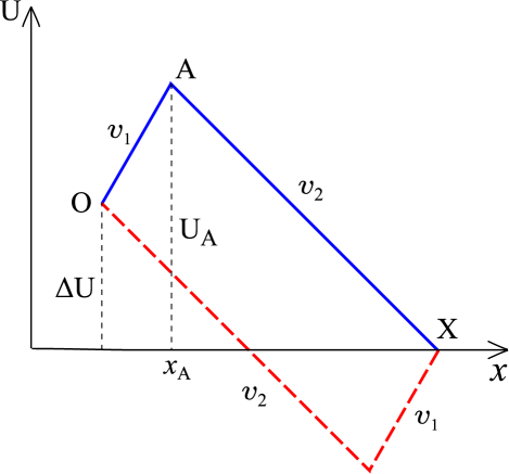
Figure 1: Sketch of a piecewise linear potential between the initial particle position in point O and the target point X. Initially the particle needs to cross the potential barrier culminating in A fuelled by thermal fluctuations, before a constant downward slope pushes the particle towards X. The same result is obtained by first sliding down and then crossing the barrier (red dashed lines).

The basis for the analytical description of this subdiffusion problem with given distribution (2) of waiting times $\tau$ in the long-time limit $t\gg\tau^{\star}$ is given by the fractional Fokker-Planck equation [3] which we here write in the integral form

$$P(x,t)-P(x,0)=\,_{0}D^{-\alpha}_{t}\left(\frac{\partial}{\partial x}\frac{U^{\prime}(x)}{m\eta_{\alpha}}+K_{\alpha}\frac{\partial^{2}}{\partial x^{2}}\right)P(x,t)$$ (3)

where $P(x,0)$ is the initial condition, $U^{\prime}(x)$ is the derivative of the external potential, $m$ is the particle mass, and $\eta_{\alpha}$ the friction experienced by the particle. The Riemann-Liouville fractional integral is defined in terms of

$${}_{0}D^{-\alpha}_{t}P(x,t)=\frac{1}{\Gamma(\alpha)}\int_{0}^{t}\frac{P(x,t^{\prime})}{(t-t^{\prime})^{1-\alpha}}dt^{\prime},$$ (4)

representing a Laplace convolution. In the Brownian limit $\alpha=1$, Eq. (3) reduces to the regular Fokker-Planck equation.

For segments with a linear potential in our piecewise linear form $U=m\eta_{\alpha}v_{i}$ the fractional Fokker-Planck equation reduces to

$$P_{i}(x,t)-P_{i}(x,0)=\,_{0}D^{-\alpha}_{t}\left(-v_{i}\frac{\partial P_{i}(x,t)}{\partial x}+K_{\alpha}\frac{\partial^{2}P_{i}(x,t)}{\partial x^{2}}\right),$$ (5)

where $i=1,2$ corresponds to the two different slopes of the piecewise linear potential. In our choice of $U$ the $v_{i}$ correspond to drift velocities, as the dimension of $\eta_{\alpha}$ is that of $[\eta_{\alpha}]=\mathrm{sec}^{\alpha-2}$ [3]. The solution of this equation with a reflective boundary condition at one end and an absorbing boundary at the other can be found by methods similar to the Brownian case, compare Ref. [1]. If both boundary and initial conditions are set as vanishing probability at $x_{X}=1$, $P(1,t)=0$, for the absorbing boundary, the flux condition at the origin $x_{\mathrm{O}}=0$ of the form $j(0,t)=\frac{\partial P(0,t)}{\partial x}-vP(0,t)=\delta(t)$, and the initial condition $P(x,0)=0$ [1], then

$$P_{i}(x,t)=\,_{0}D^{-\alpha}_{t}\left(K_{\alpha}\frac{\partial^{2}P_{i}(x,t)}{\partial x^{2}}-v_{i}\frac{\partial P_{i}(x,t)}{\partial x}\right).$$ (6)

Applying the Laplace transform

$$P(x,s)=\int_{0}^{\infty}P(x,t)e^{-st}dt$$ (7)

to Eq. (6), we find the ordinary differential equation

$$s^{\alpha}P_{i}(x,s)=\left(K_{\alpha}\frac{\partial^{2}P_{i}(s,t)}{\partial x^{2}}-v_{i}\frac{\partial P(s,t)}{\partial x}\right).$$ (8)

The solution of this equation has the form $P(x,t)=A_{i}e^{\alpha_{i}x}+B_{i}e^{\beta_{i}x}$ with the exponents

$$\alpha_{1,2} = \left(v_{1,2}+\sqrt{v_{1,2}^{2}+4K_{\alpha}s^{\alpha}}\right)/2K_{\alpha},$$

$$\beta_{1,2} = \left(v_{1,2}-\sqrt{v_{1,2}^{2}+4K_{\alpha}s^{\alpha}}\right)/2K_{\alpha}.$$ (9)

The coefficients $A_{1,2}$ and $B_{1,2}$ are determined by the boundary conditions $P(1,t)=0$ and $j(0,t)=\delta(t)$ as well as by the continuity of flux and distribution $P$ at $x=x_{\mathrm{A}}$. This produces the following system of linear equations,

$$A_{1}v_{1}+B_{1}v_{1}-K_{\alpha}\alpha_{1}A_{1}-K_{\alpha}\beta_{1}B_{1}=1$$

$$A_{2}e^{-\alpha_{2}}+B_{2}e^{-\beta_{2}}=0$$

$$A_{1}e^{-\alpha_{1}x_{\mathrm{A}}}+B_{1}e^{-\beta_{1}x_{\mathrm{A}}}=A_{2}e^{-\alpha_{2}x_{\mathrm{A}}}+B_{2}e^{-\beta_{2}x_{\mathrm{A}}}$$

$$A_{1}v_{1}e^{-\alpha_{1}x_{\mathrm{A}}}+B_{1}v_{1}e^{-\beta_{1}x_{\mathrm{A}}}-K_{\alpha}\alpha_{1}A_{1}e^{-\alpha_{1}x_{\mathrm{A}}}-K_{\alpha}\beta_{1}B_{1}e^{-\beta_{1}x_{\mathrm{A}}}$$

$$\hskip 22.76228pt=A_{2}v_{2}e^{-\alpha_{2}x_{\mathrm{A}}}+B_{2}v_{2}e^{-\beta_{2}x_{\mathrm{A}}}-K_{\alpha}\alpha_{2}A_{2}e^{-\alpha_{2}x_{\mathrm{A}}}-K_{\alpha}\beta_{2}B_{2}e^{-\beta_{2}x_{\mathrm{A}}}.$$ (10)

Due to the divergence of the characteristic waiting time $\langle\tau\rangle$ for CTRW subdiffusion processes, even in confined geometries no mean first passage time exists [10, 11]. Below we will therefore analyse the average time for the 50% or 90% probability that the particle has arrived in X. Analytically, the relevant quantity for this type of process is the probability density of first arrival, $\wp_{\alpha}(t)$, or the cumulative survival probability, $\mathscr{S}_{\alpha}(t)=\int_{0}^{1}P(x,t)dx$. Both quantities are related through $\wp_{\alpha}(t)=-d\mathscr{S}_{\alpha}(t)/dt$ [1]. In our case of the absorbing boundary condition at X we obtain the first passage density in terms of the flux at $x=\mathrm{X}$ ($=1$ in our units). In Laplace space,

$$\wp_{\alpha}(s)=j(1,s)=-K_{\alpha}\alpha_{2}A_{2}e^{-\alpha_{2}x_{\mathrm{A}}}-K_{\alpha}\beta_{2}B_{2}e^{-\beta_{2}x_{\mathrm{A}}}$$ (11)

in terms of the exponents and coefficients defined in Eqs. (9) and (10).

We note that for CTRW subdiffusion any process described by the fractional Fokker-Planck equation (5) can be related to its Brownian counterpart simply by the method of subordination, i.e., a transformation of the number of steps to the process time. For the first passage process this subordination corresponds to the Laplace space rescaling [3]

$$\wp_{\alpha}(s)=\wp_{1}\left(s^{\alpha}\frac{\eta_{\alpha}}{\eta_{1}}\right),$$ (12)

where the factor $\eta_{\alpha}/\eta_{1}$ takes care of the dimensionality: $[\eta_{\alpha}/\eta_{1}]=\mathrm{sec}^{\alpha}$.

From the above expressions in Laplace space we now perform a numerical Laplace inversion [12] and compare the obtained results to simulations of the CTRW process in the external, piecewise linear potential $U$.

3 Numerical analysis and Monte Carlo simulations

Figure 2: Mean first passage time for the 50% (left) and 90% (right) probability of particles having arrived to X, as function of the potential amplitudes $U_{\mathrm{A}}$. The green curves (top curve on the left, bottom curve on the right) correspond to the analytical result for normal diffusion ($\alpha=1$), see Ref. [2]. The red (centre) curves and triangles represent the numerical Laplace inversion of Eq. (11) and simulations results for $\alpha=0.75$, respectively. The blue curves and squares stand for $\alpha=0.5$. Lattice size for the CTRW was $N=1001$ and $x_{\mathrm{A}}=0.1\mbox{ cm}$. Each symbol represents $10^{5}$ simulation runs.

The Monte Carlo simulations of the CTRW process were performed on a lattice with $N=1001$ points and the waiting times in between successive jumps were drawn from a waiting time with asymptotic power-law decay, $\psi(t)\simeq t^{-1-\alpha}$ with $0<\alpha<1$, for details see Ref. [13]. In the chosen units the length of the interval $\overline{\mathrm{OX}}$ is $1\mbox{ cm}$, and thus the lattice constant is $\Delta x=\overline{\mathrm{OX}}/N$. For comparison with the simulations we make use of the explicit derivation of the FFPE [3, 14], such that in the limit $\tau^{\star}\to 0$ and $\Delta x\to 0$ we have

$$K_{\alpha}\approx\frac{1}{2N^{2}\tau^{\alpha}},$$

$$|v_{1}|\approx\frac{U_{\mathrm{A}}}{2x_{\mathrm{A}}N^{2}k_{B}T_{M}\tau^{\alpha}},$$

$$|v_{2}|\approx\frac{U_{\mathrm{A}}}{2(1-x_{\mathrm{A}})N^{2}k_{B}T_{M}\tau^{\alpha}},$$ (13)

where $k_{B}$ is the Boltzmann factor and $T$ the (Monte-Carlo simulations) temperature. For simplicity we use $K_{\alpha}=1\,\mathrm{cm}^{2}/\mathrm{sec}^{\alpha}$.

Results are shown in Fig. 2 for the 50% and 90% probability of particle absorption at the target point X. For each case we show results for the cases $\alpha=1/2$ and $\alpha=3/4$, as well as include the analytical result for the Brownian case from Ref. [2]. In these simulations the potential maximum was placed at $x_{\mathrm{A}}=0.1\mbox{ cm}$. Moreover, the potential at the starting and end points was chosen as zero: $U_{\mathrm{O}}=U_{\mathrm{X}}=0$. The lines for the subdiffusive cases were obtained from numerical Laplace inversion of Eq. (11) and subsequent integration such that the plotted times $t_{50}$ and $t_{90}$ are implicitly defined through the integral $\int_{0}^{t_{50}}\wp_{\alpha}(t)dt=0.5$, and analogously $=0.9$ for $t_{90}$. The symbols are obtained from the Monte Carlo simulations.

Fig. 2 shows some remarkable properties. Thus, for the case of the 90% probability the Brownian case exhibits the shortest absorption times, and the subdiffusive cases with $\alpha=3/4$ and $\alpha=1/2$ become increasingly slower. This result would be naively expected. However, for the 50% probability the behaviour is exactly opposite, i.e., the 50% first passage is fastest for the most pronounced subdiffusion. This effect is due to the fact that one-sided stable distributions, to which our waiting time distribution $\psi(t)$ belongs, have long power-law tails, but are also more concentrated around the origin at $t=0$. Thus, if we cut off extremely long waiting times governed by the long tail of $\psi(t)$ (particles that do not arrive up to $t_{50}$), we actually observe that the resulting process becomes faster for decreasing $\alpha$. At 90% probability this trend is inverted, as the statistics include sufficiently many long(er) waiting times.

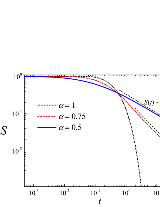
Figure 3: Survival probability as function of time $t$ for the Brownian case and stable exponents $\alpha=0.5$ and $\alpha=0.75$. While for $\alpha=1$ the decay of $\mathscr{S}_{\alpha}(t)$ is exponential, for the subdiffusive cases a power-law behaviour is observed as $t\to\infty$. Before the crossover at $t\approx 1$ the decay of the subdiffusive particles is faster than the Brownian particle. Parameters: $U_{\mathrm{A}}=2k_{B}T$ and $x_{\mathrm{A}}=0.1\mbox{ cm}$.

The second important observation is that the minima of all first passage time curves in Fig. 2 are located at $U_{\mathrm{A}}\approx 2.2k_{B}T$ for all $\alpha$ as well as for 50% and 90% probability. Thus, if a certain value $U_{\mathrm{A}}$ optimises the first passage behaviour for a Brownian particle, it also optimises the corresponding subdiffusive dynamics.

These findings are corroborated by the functional behaviour of the survival probability $\mathscr{S}(t)$, as shown in Fig. 3. At smaller times, corresponding to a smaller percentage of the probability of first passage, indeed the decay is faster for more pronounced subdiffusion and slowest for normal diffusion. Approximately at unit time $t=1$ a crossover is observed, and for longer times we find the naively expected behaviour: Brownian motion effects the fastest decay while the subdiffusive motion is slower. At long times $t\rightarrow\infty$ the survival probability for the subdiffusive cases exhibits the power law $\mathscr{S}_{\alpha}(t)\sim t^{-\alpha}$, compare Refs. [3, 10, 11]. This follows directly from the subordinated exponential decay of Brownian motion also shown in Fig. 3.

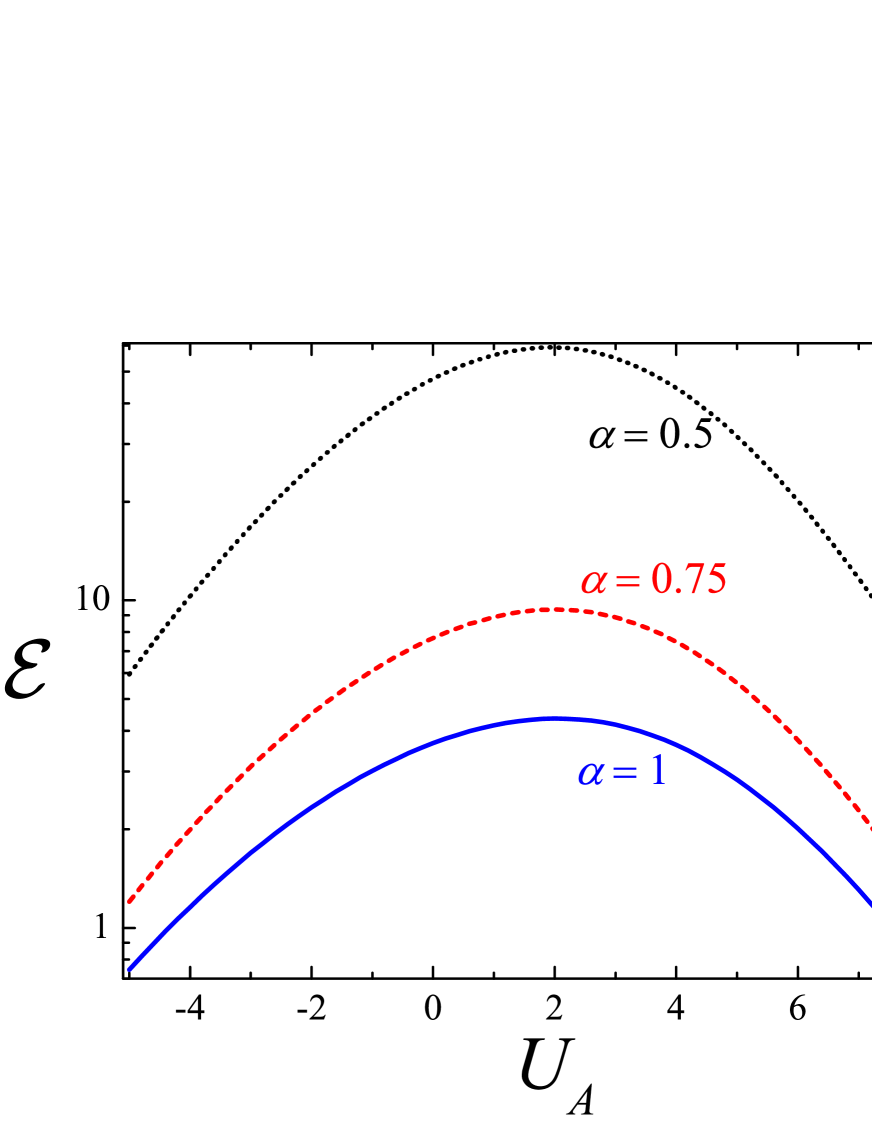
Figure 4: Dependence of the efficiency $\mathcal{E}$ on the value $U_{\mathrm{A}}$ of the potential at the maximum point A, for different positions of point A, $x_{\mathrm{A}}=0.1\mbox{ cm}$ (left, asymmetric potential) and $x_{\mathrm{A}}=0.5$ cm (right, symmetric potential).

Yet another way to characterise the first passage behaviour is to evaluate the average rate $\left<1/t\right>$, which was introduced for superdiffusive search as a non-diverging measure of optimisation [15, 16]. This quantity can be computed conveniently numerically via the relation

$$\mathcal{E}=\left\langle\frac{1}{t}\right\rangle=\int_{0}^{\infty}\wp_{\alpha}(s)ds$$ (14)

from the Laplace space result of the first passage density $\wp_{\alpha}(t)$. The functional form of this quantity shows another remarkable property: even in the absence of a potential the efficiency $\mathcal{E}$ increases with decreasing stable exponent $\alpha$. Namely, using the known result for normal Brownian diffusion [1], from subordination we find that for $U(x)=0$

$$\wp_{\alpha}(s)=2\frac{\sinh\left(L\sqrt{s^{\alpha}/D}\right)}{\sinh\left(2L\sqrt{s^{\alpha}/D}\right)}=\frac{1}{\cosh\left(L\sqrt{s^{\alpha}/D}\right)}$$ (15)

Therefore,

$$\mathcal{E}=\int_{0}^{\infty}\cosh\left(L\sqrt{s^{\alpha}/D}\right)ds\sim C+\int_{0}^{\infty}e^{-Ls^{\alpha/2}/\sqrt{D}}ds,$$ (16)

where $C$ is a constant. In the limit $\alpha\rightarrow 0$ this expression reduces to

$$\mathcal{E}\approx\Gamma\left(\frac{2}{\alpha}\right),$$ (17)

which proves the fact that the average rate increases with the decrease of the stable exponent $\alpha$. In the case of the piecewise linear potential this behaviour is indeed preserved, as shown in Fig. 4. The figure also demonstrates that the maxima of the efficiency are consistent with the minima of the 50% and 90% probability first passage times, $t_{50}$ and $t_{90}$ shown in Fig. 2. Note that even in the case of a symmetric potential shown on the right of Fig. 4 the first passage dynamics profits from the existence of the energy landscape: after crossing the peak the diffusion back towards the starting point O is suppressed.

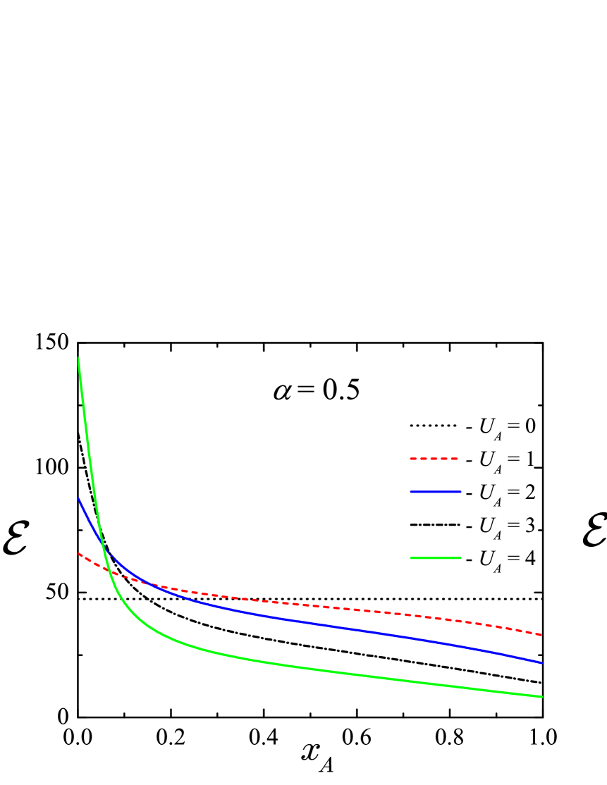
Figure 5: Efficiency $\mathcal{E}$ as function of the position $x_{\mathrm{A}}$ of the potential maximum with fixed value $U_{\mathrm{A}}$. Note the crossover at small values of $x_{\mathrm{A}}$. A higher potential peak $U_{\mathrm{A}}$ facilitates the first passage as long as the peak location $x_{\mathrm{A}}$ remains close to the starting point O. The dotted line indicates the efficiency value in absence of an external potential, i.e., $U_{\mathrm{A}}=0$.

The dependence of the efficiency $\mathcal{E}$ on the position $x_{\mathrm{A}}$ of the potential maximum is displayed in Fig. 5, for different $U_{\mathrm{A}}$ values of the potential (as indicated in the panels). Consistently for all $\alpha$ the efficiency increases with growing value $U_{\mathrm{A}}$ when $x_{\mathrm{A}}$ shifts towards the starting point O: the particle requires a larger thermal fluctuation to cross the initial peak $U_{\mathrm{A}}$, but then experiences a higher, constant drift velocity towards its target X. At growing values for $x_{\mathrm{A}}$ we observe a crossover, and then a higher peak value $U_{\mathrm{A}}$ effects lower efficiency.

What would happen if we let the particles age before sending them on their journey from O to X? Ageing is a characteristic property of subdiffusive CTRW particles: the process is highly non-stationary, and physical observables strongly depend on the ageing time $t_{a}$ elapsing between system initiation and start of the measurement [17]. Due to the scale-free form of the waiting time distribution with diverging mean waiting time $\langle t\rangle$, longer and longer waiting times occur on average, such that effectively the particle is constantly slowing down. Physically, in the picture of a random energy landscape this effect corresponds to the situation that the particle discovers deeper and deeper traps on its path. After passing the ageing period, the first step of the particle then corresponds to the forward waiting time [17, 18]

$$\psi_{t_{a}}(t_{1})=\frac{\sin(\pi\alpha)}{\pi}\frac{t_{a}^{\alpha}}{t_{1}^{\alpha}(t_{1}+t_{a})}$$ (18)

For the parameters $U_{\mathrm{A}}=3$ and $x_{\mathrm{A}}=0.1$ we show the dependence of the efficiency $\mathcal{E}$ on the ageing time $t_{a}$ of the process for the subdiffusive cases with $\alpha=1/2$ and $\alpha=3/4$. Indeed, the continued slow-down of the motion due to increase of the typical waiting times leads to a pronounced decrease of $\mathcal{E}$ of the power-law form

$$\mathcal{E}(t_{a})\simeq t_{a}^{\alpha-1},$$ (19)

corresponding to the product of the first passage density without ageing ($t_{a}=0$) and the probability density of the forward waiting time [17]. This behaviour is indeed nicely observed in our simulations, as demonstrated in Fig. 6.

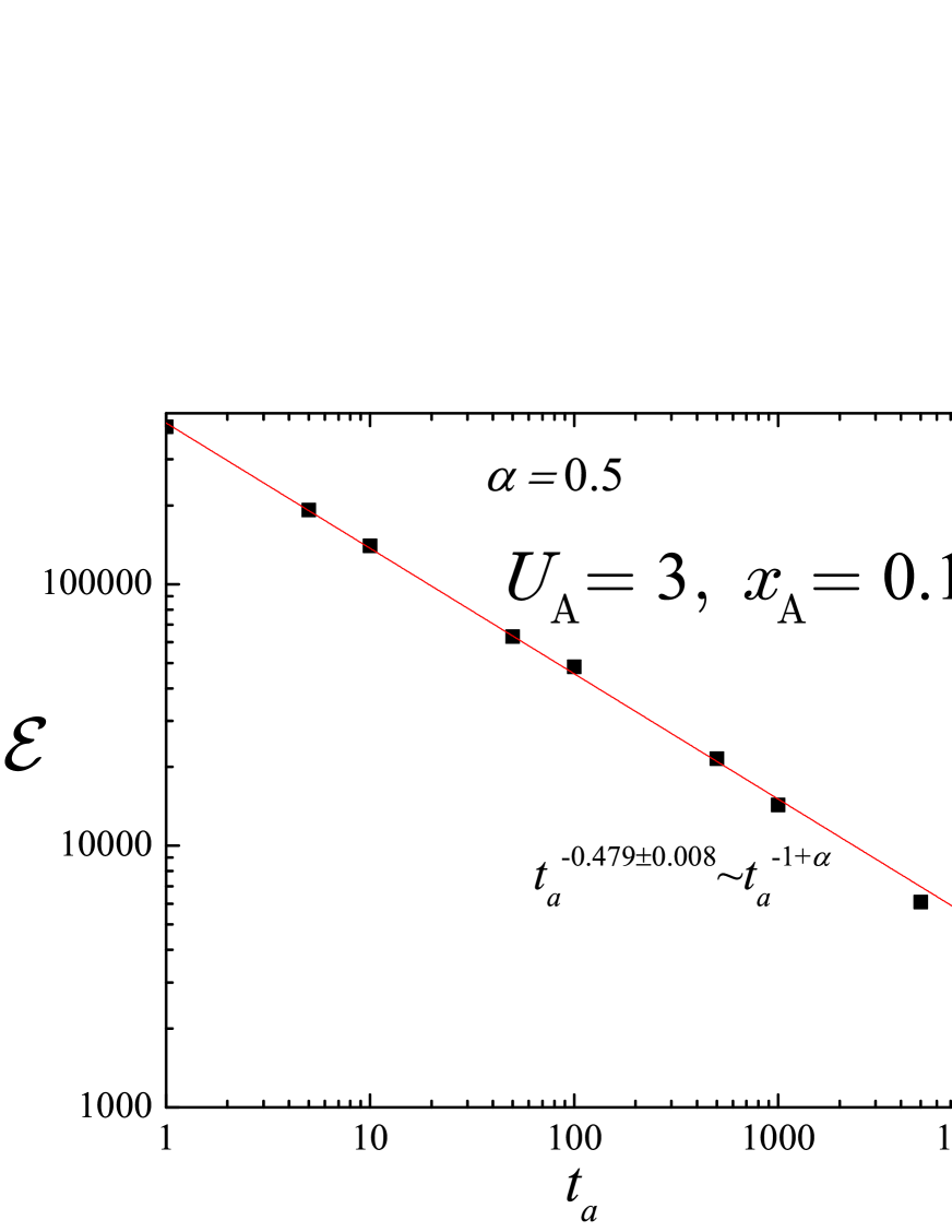
Figure 6: Dependence of the search efficiency $\mathcal{E}$ on the ageing time $t_{a}$ elapsing between initiation of the process and start of our observation of the particle at $x_{\mathrm{O}}$, for $\alpha=0.5$ (left) and $\alpha=0.75$ (right). We observe that $\mathcal{E}(t_{a})\simeq t_{a}^{\alpha-1}$, as predicted by Eq. (19). Parameters: $U_{\mathrm{A}}=3$ and $x_{\mathrm{A}}=0.1$.

4 Discussion and Conclusions

The study of the mean first passage behaviour in finite, flat potential landscapes has experienced remarkable progress during the last few years [19]. In particular, the distinction of compact versus non-compact exploration strategies led to the concept of “geometry-controlled kinetics” [20]. Moreover, the trajectory-to-trajectory variation of first passage times have been studied on finite domains of various shapes recently [21]. Much less is known about the first passage in potential landscapes.

Previously we found that for normal Brownian diffusion the first passage in a finite interval can be sped up significantly by introducing a potential landscape [2]. For the case of a piecewise linear potential, the role of the potential is intuitively clear: after crossing an initial potential barrier, the particle continuously slides down towards the target. When the position of the barrier successively approaches the point of release and the barrier height increases, the mean first passage time decreases [2].

Here we studied the behaviour in such a piecewise linear potential for the case of a subdiffusing particle whose dynamics is governed by a long-tailed waiting time distribution with a diverging characteristic waiting time. From analysis of the probability percentage of the first passage, the survival probability, and the efficiency parameter we found a number of remarkable properties. Namely, as in the Brownian case the introduction of the barrier indeed leads to a more efficient (i.e., faster) first passage behaviour for a given value $\alpha$ of the anomalous diffusion exponent. At short times, somewhat surprisingly the more subdiffusive particle performs better than the Brownian particle, while at longer times the less subdiffusive particle wins out. The optimal height of the potential barrier is thereby conserved for varying $\alpha$. Moreover, the efficiency increases dramatically when the position of the potential maximum is shifted towards the particle origin O. Finally, the ageing of the particle leads to a power-law decay of the efficiency as function of the ageing time.

As in the Brownian case [2] a faster first passage of particles through the interval $\overline{\mathrm{OX}}$ in the presence of the potential barrier does not contradict the corresponding result of the (fractional) Kramers escape [22]. The distribution of escape times for CTRW subdiffusion becomes [22]

$$\wp^{K}_{\alpha}(t)=E_{\alpha}\left(-r_{K}^{(\alpha)}t^{\alpha}\right)$$ (20)

where $E_{\alpha}$ is the Mittag-Leffler function

$$E_{\alpha}(-z)=\sum_{n=0}^{\infty}(-z)^{n}/\Gamma(1+\alpha n)$$ (21)

with $E_{\alpha}(-z)\sim 1/z$ at $z\to\infty$. The (fractional) rate coefficient $r_{K}^{(\alpha)}$ is given by

$$r_{K}^{(\alpha)}=\frac{\sqrt{U^{\prime\prime}(x_{\mathrm{min}})U^{\prime\prime}(x_{\mathrm{max}})}}{2\pi m\eta_{\alpha}}\exp\left(-\frac{\Delta U}{k_{B}T}\right).$$ (22)

Thus shifting the maximum at $x_{\mathrm{A}}$ towards point O leads to an increase of the curvatures at the maximum and minimum positions in Eq. (22), and hence speeds up the rate in the same way as observed in Ref. [2], if $U_{\mathrm{A}}$ is kept constant.

Let us briefly discuss a technologically relevant, physical application of the above results. Namely, we consider the passage of a polymer chain through a narrow channel, the so-called translocation process [23]. Indeed, in terms of the translocation co-ordinate $m$ (the number of monomers crossing the exit of the channel) the translocation becomes subdiffusive, see, for instance, Refs. [24, 25]. The fractional Fokker-Planck equation was proposed to model this subdiffusive behaviour, and shown to capture the first passage behaviour of the translocating polymer chain in comparison to simulations [26]. More recently, it has become clear that the translocation of a polymer through a narrow channel without interactions between channel wall and polymer chain is stochastically described by fractional Langevin equation motion driven by long-ranged Gaussian noise [27]. However, the long-time translocation dynamics of a polymer may still be governed by the fractional Fokker-Planck equation if the motion of the chain is successively immobilised with power-law distributed waiting times due to monomer-channel interactions or extra-channel inhibitors.

The translocation time of a polymer through a channel consists of three distinct contributions [28]: (i) the time needed for the free polymer chain on the cis side of the channel to diffuse to the channel entrance, (ii) the time for one of the chain ends to thread into the channel entrance, and (iii) the passage of the chain through the channel across the entropic potential describing the reduction of the polymer’s accessible degrees of freedom due to the imposed constraints plus some external driving potential. With the translocation co-ordinate $m$ for a polymer with $N$ monomers, this gives rise to the free energy landscape [29]

$$\mathcal{F}(m)=-k_{B}T\left(N\ln\mu+\left(\gamma_{1}-1\right)\ln\left[(N-m)m\right]\right),$$ (23)

where $\mu$ is the (non-universal) lattice connectivity (e.g., $\mu=6$ on a cubic lattice) and $\gamma_{1}$ is the topological critical exponent for a self-avoiding chain attached to a wall, $\gamma_{1}=0.680$ for a self-avoiding chain in three dimensions. For translocation processes only the second term of the free energy function (23) depends on the translocation co-ordinate $m$ and thus matters to our analysis. The entropic free energy barrier in Eq. (23) clearly slows down the translocation of the chain. In the mathematical description in the pseudo-equilibrium approximation [28, 29, 30], we are only interested in the very translocation dynamics of the chain, and we therefore impose a reflecting boundary condition at $x=0$, in order to prevent the chain from escaping the channel.

Figure 7: Potential landscape for translocation of a gradient copolymer in the quasi-equilibrium approximation. The black line depicts the entropic contribution of the polymer chain. The red line is the piecewise linear potential, which characterises the interactions, see text. The blue curve is the sum of these contributions which represents the actual potential for the translocation process.

What happens when instead of a homogeneous polymer chain we consider a gradient or tapered copolymer with a a sequence of monomers of different types with different monomer-channel interactions? Gradient copolymers show a quite special behaviour with respect to their thermodymamic properties, contrasting other copolymer sequences [31, 32, 33, 34]. The effects of interactions between translocating chain and channel were indeed studied previously for the passage of heteropolymers Refs. [35]. To demonstrate the possibility of modifying the translocation time statistics for such inhomogeneous polymer chains we imagine a polymer sequence, that gives rise to a piecewise linear potential of the shape studied above. Combining this with the translocation free energy (23), we obtain the landscape portrayed in Fig. 7.

Simulations of this modified translocation process produce the 50% and 90% probabilities for translocation across the combined free energy landscape shown in Fig. 8. Evidently the piecewise linear potential can lower the translocation time. As above, the position of the optimum (at around $U_{\mathrm{A}}\approx 1.5k_{B}T$, different from the value without the entropic potential) is independent of the exponent $\alpha$ and whether we consider the 50% or 90% case. Notably, while the overall translocation times are higher in the 90% case, the effect of the potential is strongest for $\alpha=1/2$.

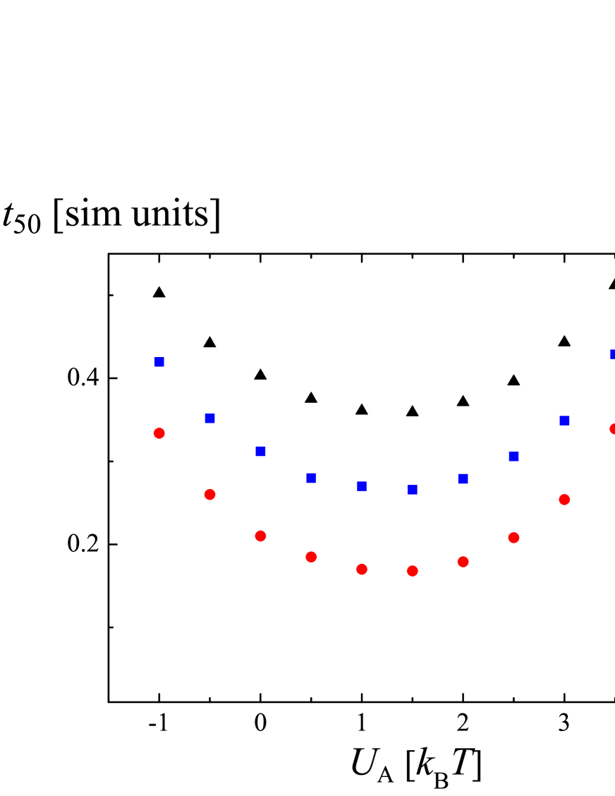
Figure 8: Simulated translocation times with 50% and 90% translocation probability for the combined free energy landscape of Fig. 7 for a chain with $N=1001$ monomers. The maximum of the piecewise linear potential component is at $x_{\mathrm{A}}=100$. Black triangles show the simulations results for $\alpha=0.5$, blue squares for $\alpha=0.75$, and red circles for the Brownian case. $10^{5}$ simulation runs were performed to obtain the data points.

Thus the sequence of the copolymer may have a significant influence on the translocation times. This statement itself was already confirmed by Monte-Carlo simulations Ref. [36], in which the authors found a distinct variation of up to 3 orders of magnitude in translocation times for different sequences but same composition. However, they did not report the effect of decreased translocation times in comparison with the homopolymer by adding slower translocating segments. We mention that an essential part of this brief discussion relies on the quasi-equilibrium approximation, necessary to apply a free energy picture [24], which was shown to be inapplicable in many cases of translocation [24, 37]. However, we assume that these effects on polymer translocation times will remain relevant for non-equilibrium situations, as well. It is feasible that parts of biopolymer sequences may have gradient or tapered parts which assist translocation. These specific interaction potentials may also originate from combination of complex pore structure and copolymer sequence as in Refs. [35]. Further studies of this problem are expected to shed new light on the biophysics of translocation processes.

References

References

- [1] S. Redner, A Guide to First-Passage Processes (Cambridge University Press, Cambridge, UK, 2001).
- [2] V.V. Palyulin and R. Metzler, J. Stat. Mech., L03001 (2012).
- [3] R. Metzler and J. Klafter, Phys. Rep. 339, 1 (2000); J. Phys. A 37, R161 (2004).
- [4] E. W. Montroll and G. H. Weiss, J. Math. Phys. 6, 167 (1965).
- [5] H. Scher and E. W. Montroll, Phys. Rev. B 12, 2455 (1975).
- [6] J. Klafter and I. M. Sokolov, First Steps in Random Walks (Cambridge University Press, Cambridge UK, 2012).
-
[7]
S. M. A. Tabei, S. Burov, H. Y. Kim, A. Kuznetsov, T. Huynh, J.
Jureller, L. H. Philipson, A. R. Dinner, and N. F. Scherer, Proc. Natl. Acad.
Sci. USA 110, 4911 (2013).
J.-H. Jeon, V. Tejedor, S. Burov, E. Barkai, C. Selhuber-Unkel, K. Berg-Sørensen, L. Oddershede, and R. Metzler, Phys. Rev. Lett. 106, 048103 (2011). - [8] Y. Wong, M. L. Gardel, D. R. Reichman, E. R. Weeks, M. T. Valentine, A. R. Bausch, and D. A. Weitz, Phys. Rev. Lett. 92, 178101 (2004).
- [9] Q. Xu, L. Feng, R. Sha, N. C. Seeman, and P. M. Chaikin, Phys. Rev. Lett. 106, 228102 (2011).
- [10] R. Metzler and J. Klafter, Physica A 278, 107 (2000).
- [11] S.B. Yuste, K. Lindenberg, Phys. Rev. E, 69, 033101 (2004).
- [12] For numerical Laplace inversion the additional package by P. P. Valkó and J. Abate was used in Mathematica: http://library.wolfram.com/infocenter/Demos/4738/; P.P. Valkó and J. Abate, Comput. Math. Appl., 48, 629 (2004).
- [13] J. M. Chambers, C. L. Mallows, B. W. Stuck, Journal of the American Statistical Association, 71, 340 (1976).
- [14] R. Metzler, E. Barkai, and J. Klafter, Europhys. Lett.
- [15] V.V. Palyulin, A.V. Chechkin and R. Metzler, arXiv:1306.1181
- [16] V.V. Palyulin, A.V. Chechkin and R. Metzler, in preparation.
-
[17]
J.-P. Bouchaud, J. Phys. I (Paris) 2, 1705 (1992).
C. Godrèche and J. M. Luck, J. Stat. Phys. 104, 489 (2001).
E. Barkai, Phys. Rev. Lett. 90 104101 (2003).
E. Barkai, Y.-C. Cheng, J. Chem. Phys. 118 6167 (2003).
J. Schulz, E. Barkai, and R. Metzler, Phys. Rev. Lett. 110, 020602 (2013); E-print arXiv:1310.1058. - [18] T. Koren, M. A. Lomholt, A. V. Chechkin, J. Klafter, and R. Metzler, Phys. Rev. Lett. 99, 160602 (2007).
- [19] S. Condamin, O. Bénichou, V. Tejedor, R. Voituriez, and J. Klafter, Nature 450, 77 (2007).
- [20] O. Bénichou, C. Chevalier, J. Klafter, B. Meyer, and R. Voituriez, Nature Chem. 2, 472 (2010).
-
[21]
C. Mejía-Monasterio, G. Oshanin, and G. Scher, J. Stat. Phys.
2011, P06022.
T. G. Mattos, C. Mejía-Monasterio, R. Metzler, and G. Oshanin, Phys. Rev. E 86, 031143 (2012). - [22] R. Metzler, and J. Klafter, Chem. Phys. Lett. 321 238 (2000).
- [23] A. Meller, J. Phys. Cond. Mat. 15, R581 (2003).
-
[24]
J. Chuang, Y. Kantor, and M. Kardar, Phys. Rev. E,
65 011802 (2001).
Y. Kantor, and M. Kardar, Phys. Rev. E, 69 021806 (2004). - [25] K. Luo, T. Ala-Nissilä, S.-Ch. Ying, and R. Metzler, Europhys. Lett. 88, 68006 (2009).
-
[26]
J. L. A. Dubbeldam, A. Milchev, V. G. Rostiashvili, and T. A.
Vilgis, Phys. Rev. E,76 010801(R) (2007).
J. L. A. Dubbeldam, A. Milchev, V. G. Rostiashvili, and T. A. Vilgis, EPL, 79 18002 (2007).
R. Metzler and J. Klafter, Biophys. J. 85, 2776 (2003). - [27] D. Panja, G. T. Barkema, and A. B. Kolomeisky, J. Phys. Cond. Mat. 25m 413101 (2013).
- [28] M. Muthukumar, J. Chem. Phys., 132, 195101 (2010).
- [29] M. Muthukumar, J. Chem. Phys., 111, 10371 (1999).
- [30] R. Metzler and K. Luo, Euro. Phys. J. ST 189, 119 (2010).
- [31] U. Beginn, Colloid. Polym. Sci., 286 1465 (2010).
- [32] K. U. Claussen, T. Scheibel, H.-W. Schmidt, and R. Giesa, Macromol. Mater. Eng., 297 938 (2012).
- [33] V. V. Palyulin and I. I. Potemkin, J. Chem. Phys., 127 124903 (2007)
- [34] S. Okabe, K. Seno, S. Kanaoka, S. Aoshima, and M. Shibayama, Macromolecules 39 1592 (2006).
-
[35]
J.A. Cohen, A. Chandhuri and R. Golestanian, Phys. Rev. X,
2, 021002 (2012).
R. H. Abdolvahab, R. Metzler, and M. R. Ejtehadi, J. Chem. Phys. 135, 245102 (2011).
K. Luo, T. Ala-Nissila, S.-C. Ying and A. Bhattacharya, J. Chem. Phys. 126, 145101 (2007). - [36] M.G. Gauthier and G.W. Slater, J. Chem. Phys., 128 175103 (2008).
- [37] T. Sakaue, Phys. Rev. E, 76, 021803 (2007).