Two multilayered plate models with transverse shear warping functions issued from three dimensional elasticity equations

Abstract

A multilayered plate theory which uses transverse shear warping functions is presented. Two methods to obtain the transverse shear warping functions from three-dimensional elasticity equations are proposed. The warping functions are issued from the variations of transverse shear stresses computed at specific points of a simply supported plate. The first method considers an exact 3D solution of the problem. The second method uses the solution provided by the model itself: the transverse shear stresses are computed integrating equilibrium equations. Hence, an iterative process is applied, the model is updated with the new warping functions, and so on. Once the sets of warping functions are obtained, the stiffness and mass matrices of the models are computed. These two models are compared to other models and to analytical solutions for the bending of simply supported plates. Four different laminates and a sandwich plate are considered. Their length-to-thickness ratios vary from 2 to 100. An additional analytical solution that simulates the behavior of laminates under the plane stress hypothesis – shared by all the considered models – is computed. Both presented models give results very close to this exact solution, for all laminates and all length-to-thickness ratios.

1 Introduction

In many human-built structures, plates and shells are present. These particular structures are distinguished from others because a dimension – the transverse dimension – is much smaller than the others. Hence, although it is always possible, their representation through a three-dimensional domain is not the best way to study them. To understand and predict their mechanical behavior, plate models have been developed. These models permit to study plates and shells through a two-dimensional domain while allowing at least membrane and bending deformations. What happens in the third direction is not ignored, it is precisely the purpose of the plate model to integrate the transverse behavior into its equations. The better this behavior is described, the more accurate the model will be. History of plate models probably begins with works of Kirchhoff, Love, and Rayleigh [1, 2, 3] leading to the Love-Kirchhoff model in which no shear deformation is allowed. Because of the limitation of this model to thin plates, authors like Reissner, Hencky, Bolle, Uflyand, and Mindlin[4, 5, 6, 7, 8] have proposed to integrate the shear phenomenon into their formulation. In particular, Reissner made the assumption that shear stresses have a parabolic distribution and consider the normal stress in his model which is derived from a complementary energy. On the other hand, Hencky and Mindlin considered a linear variation of the displacements $\displaystyle u$ and $\displaystyle v$ and no transverse strain. Mindlin and Reisnner theories are often associated but it is incorrect as demonstrated in reference [9]. The Love-Kirchhoff and the Hencky–Mindlin models were first proposed for homogeneous plates but their pendent for laminated structures have been later presented and are called the Classical Laminated Plate Theory (CLPT) and the First-order Shear Deformation laminated plate Theory (FoSDT). The last one has been improved by the use of shear correction factors [10, 11, 12]. The need to improve this accuracy has been motivated by the study of thick plates and laminated plates. In both cases, the early plate models fail to give accurate results. It is even worse if some layers have low mechanical properties compared to others, which is the case for sandwich structures or when viscoelastic layers are used to improve the damping. To overcome these difficulties, specific models have been proposed. However, a universal model that can manage plates of various length-to-thickness ratios, with any lamination scheme and various materials including functionally graded materials, with good accuracy for the static, dynamic, and damped dynamic behaviors is still a challenge.

Dealing with multilayered plates has given rise to another class of theories, called the Layer-Wise (LW) models, in which the number of unknowns depends on the number of layers, by opposition to the Equivalent Single Layer (ESL) family of models in which the number of unknowns is independent of the number of layers. Obviously, LW models are expected to be more accurate than ESL models but they are less easy to implement for complex structures and require more computational resources than ESL models. This has motivated researchers to propose ESL models in which the transverse shear is taken into account in a more precise way than for the first models. With the help of the classification given by Carrera [13] among other review papers, we can distinguish different approaches that have given interesting ESL models:

• Higher-order (and also non-polynomial) shear deformation theories: the Vlasov–Levinson–Reddy [14, 15, 16] theory, also called Third order Shear Deformation Theory (ToSDT), among other third order theories, proposes a kinematic field with a third-order polynomial dependence on $\displaystyle z$, motivated by the respect of the nullity of transverse shear at top and bottom faces of the plate. Higher order (order greater than 3) theories have been proposed. Non-polynomial functions have also been used to take into account the shear phenomenon: for example, Touratier in reference [17], uses a $\displaystyle f(z)=h/\pi\sin(\pi z/h)$ function, Soldatos [18] uses a $\displaystyle f(z)=z\cosh(1/2)-h\sinh(z/h)$ function, and Thai & al. [19] uses a $\displaystyle f(z)=h\arctan(2z/h)-z$ function to integrate the transverse shear in the kinematic field. Note that, for the study of laminated plates, these models do not integrate information about the lamination sequence in their kinematic field, and do not verify the transverse stress continuity at interfaces.

• Interlaminar continuous ESL models: some a priori LW models reduce to ESL models with the help of assumptions between the fields in each layer. Zig-Zag (ZZ) models enter in this category. Pioneering works of Lekhnitskii [20] and Ambartsumyan [21] have been classified as such by Carrera [13] who also shows that other authors have integrated the multilayer structure in their model [22, 23, 24] in a very similar manner. The main idea of ZZ models is to let in-plane displacements vary with $\displaystyle z$ according to the superposition of a zig-zag law to a global law – cubic for example. With these models, shear stresses can satisfy both continuity at interfaces and null (or prescribed) values at top and bottom faces of the plate. An enhancement of the second model presented in reference [23] for general lamination sequences is proposed in references [25, 26]. Models of references [26, 24] are used for comparison in this study, they are presented at section 5.2. Other works can be cited. For example, Pai [12] presents a method to determine four warping functions of cubic order in each layer, and also a generic method to compute shear correction factors. In ref. [27], the author proposes a warping function for beam problems which is a linear ZZ function superimposed to an overall sine function. In ref. [28], the authors develop an enhancement of the model given in ref. [24] for general lamination sequences. Note that references [26, 24, 12, 28] propose models with four WF, which is necessary for the study of general lamination sequences.

• Direct approaches and micropolar plate theories: based on the works of the Cosserat brothers [29] on generalized continuum mechanics and on deformable lines and surfaces. The micropolar theory of elasticity, which considers (microscopic) continuous rotations and couples in addition to the classical displacements and forces, has been applied to rods and shells by Ericksen [30]. Later, it has been used in numerous works, including plate models, as it can be seen in the review paper [31].

• Sandwich theories: sandwich panels have been early considered apart from laminated composite because of their particular structure. They are made of two face layers (themselves made of one or several layers) and a core layer. The thickness of the faces is small compared to the thickness of the core (typically 10 times less) and Young modulus of the faces is high compared to Young modulus of the core (typically more than 1000 times higher). For these reasons, specific models have been proposed, for example by Reissner [32], followed by many others, as it can be seen in the review papers [33, 34].

Additional references can be found in recent reviews on the subject [35, 34, 36].

When theories are issued from assumptions on displacement or stress fields, there is no guarantee for these theories to be consistent. This means that, with respect to the required order of the considered theory, some terms of the three/dimensional strain energy may appear with an erroneous coefficient, or may even be omitted. The consistency of plate theories has been discussed by many authors, one can for example refer to recent works [37, 38]. Precise rules for the consistency are formulated for homogeneous materials, but it seems difficult to extrapolate them for inhomogeneous materials like laminates and sandwiches, especially when advanced kinematic and/or static assumptions are made. Although this subject is not treated in this study, it can be a significant aspect as it is mentioned in the conclusion.

In this work, the kinematic assumptions are similar of those taken in Ref. [28] but they differ because the choice of the functions describing the transverse behavior is not made a priori. These functions, called warping functions (WF) are the core of the model. The model has been entirely formulated in [26] and it has been shown that, according to specific choices of the WF, it can also represent most of the classical models (CLPT, FoSDT, ToSDT) and others, as it will appear in the following. However, and it is precisely the subject of this article, it is possible to choose and adapt the WF in a completely free manner.

This article presents two different ways of obtaining new sets of WF issued from three dimensional elasticity laws. The first way consists in building the WF from three-dimensional solutions. Three-dimensional solutions for the bending of laminates have been first obtained by Pagano and by Srinivas & al. [39, 40] for cross-ply laminates, by Noor & Burton [41] for antisymmetric angle-ply laminates, and have been recently obtained for general lamination schemes [42]. These solutions are achieved for particular boundary conditions and load, which can be seen as the principal limitation of their use in the present model. The second way is to derive the WF from the equilibrium equations. This leads to an iterative model: starting with “classical” WF, for example Reddy’s formula, WF are issued from the equilibrium equations and then integrated to the model, and so on until no significant changes are detected.

2 Considered plate theory

In this section, we recall the main components of the theory presented in Ref. [26]. It is a plate theory based on the use of transverse shear WF. It allows the simulation of multilayer laminates made of orthotropic plies using different sets of transverse shear WF. The purpose of this paper is to propose enhanced WF issued from 3D elasticity equations (see section 3), but several plate models (among ESL and ZZ models) issued from the literature can also be formulated in terms of transverse shear WF, as it was shown in Ref. [26]. This is of practical interest when comparing results issued from different models, because these models can be implemented in a similar manner.

2.1 Laminate definition and index convention

The laminate, of height $\displaystyle h$, is composed of $\displaystyle N$ layers. All the quantities will be related to those of the middle plane which is placed at $\displaystyle z=0$; they are marked with the superscript $\displaystyle 0$. In the following, Greek subscripts take values $\displaystyle 1$ or $\displaystyle 2$ and Latin subscripts take values $\displaystyle 1$, $\displaystyle 2$ or $\displaystyle 3$. The Einstein’s summation convention is used for subscripts only. The comma used as a subscript index means the partial derivative with respect to the following index(ices).

2.2 Displacement field

The kinematic assumptions of the present theory are:

$$\left\{\begin{array}[]{lll}u_{\alpha}(x,y,z)&=&u_{\alpha}^{0}(x,y)-zw^{0}_{,\alpha}(x,y)+\varphi_{\alpha\beta}(z)\gamma^{0}_{\beta 3}(x,y)\\ u_{3}(x,y,z)&=&w^{0}(x,y)\end{array}\right.$$ (1)

where $\displaystyle u_{\alpha}^{0}(x,y)$, $\displaystyle w^{0}(x,y)$ and $\displaystyle\gamma^{0}_{\alpha 3}(x,y)$, are respectively the in-plane displacements, the deflection and the engineering transverse shear strains evaluated at the middle plane. The $\displaystyle\varphi_{\alpha\beta}(z)$ are the four WF. The associated strain field is derived from equation (1):

$$\displaystyle\varepsilon_{\alpha\beta}(x,y,z) \displaystyle=\varepsilon_{\alpha\beta}^{0}(x,y)-zw^{0}_{,\alpha\beta}(x,y)+\frac{1}{2}\left(\varphi_{\alpha\gamma}(z)\gamma^{0}_{\gamma 3,\beta}(x,y)+\varphi_{\beta\gamma}(z)\gamma^{0}_{\gamma 3,\alpha}(x,y)\right)$$ (2a)

$$\displaystyle\varepsilon_{\alpha 3}(x,y,z) \displaystyle=\frac{1}{2}\varphi^{\prime}_{\alpha\beta}(z)\gamma^{0}_{\beta 3}(x,y)$$ (2b)

$$\displaystyle\varepsilon_{33}(x,y,z) \displaystyle=0\phantom{\frac{1}{2}}$$ (2c)

which, with the use of Hooke’s law, leads to the following stress field:

$$\displaystyle\sigma_{\alpha\beta}(x,y,z) \displaystyle=Q_{\alpha\beta\gamma\delta}(z)\left(\varepsilon_{\gamma\delta}^{0}(x,y)-zw^{0}_{,\gamma\delta}(x,y)+\varphi_{\gamma\mu}(z)\gamma^{0}_{\mu 3,\delta}(x,y)\right)$$ (3a)

$$\displaystyle\sigma_{\alpha 3}(x,y,z) \displaystyle=C_{\alpha 3\beta 3}(z)\varphi^{\prime}_{\beta\mu}(z)\gamma^{0}_{\mu 3}(x,y)$$ (3b)

$$\displaystyle\sigma_{33}(x,y,z) \displaystyle=0$$ (3c)

where $\displaystyle Q_{\alpha\beta\gamma\delta}(z)$ are the generalized plane stress stiffnesses and $\displaystyle C_{\alpha 3\beta 3}(z)$ are the components of Hooke’s tensor corresponding to the transverse shear stiffnesses.

2.3 Static laminate behavior

The model requires introduction of generalized forces:

$$\displaystyle\big{\{}N_{\alpha\beta},M_{\alpha\beta},P_{\gamma\beta}\big{\}} \displaystyle=\int^{h/2}_{-h/2}\big{\{}1,z,\varphi_{\alpha\gamma}(z)\big{\}}\sigma_{\alpha\beta}(z)\text{d}z$$ (4a)

$$\displaystyle Q_{\beta} \displaystyle=\int^{h/2}_{-h/2}\varphi^{\prime}_{\alpha\beta}(z)\sigma_{\alpha 3}(z)\text{d}z$$ (4b)

They are then set, by type, into vectors:

$$\mathbf{N}=\begin{Bmatrix}N_{11}\\ N_{22}\\ N_{12}\end{Bmatrix},\ \mathbf{M}=\begin{Bmatrix}M_{11}\\ M_{22}\\ M_{12}\end{Bmatrix},\ \mathbf{P}=\begin{Bmatrix}P_{11}\\ P_{22}\\ P_{12}\\ P_{21}\end{Bmatrix},\ \mathbf{Q}=\begin{Bmatrix}Q_{1}\\ Q_{2}\end{Bmatrix}$$ (5)

and the same is done for the corresponding generalized strains:

$$\boldsymbol{\epsilon}=\begin{Bmatrix}\epsilon^{0}_{11}\\ \epsilon^{0}_{22}\\ 2\epsilon^{0}_{12}\end{Bmatrix},\ \boldsymbol{\kappa}=\begin{Bmatrix}-w^{0}_{,11}\\ -w^{0}_{,22}\\ -2w^{0}_{,12}\end{Bmatrix},\ \mathbf{\Gamma}=\begin{Bmatrix}\gamma^{0}_{13,1}\\ \gamma^{0}_{23,2}\\ \gamma^{0}_{13,2}\\ \gamma^{0}_{23,1}\end{Bmatrix},\ \boldsymbol{\gamma}=\begin{Bmatrix}\gamma^{0}_{13}\\ \gamma^{0}_{23}\end{Bmatrix}$$ (6)

Generalized forces are linked with the generalized strains by the $\displaystyle 10\times 10$ and $\displaystyle 2\times 2$ following stiffness matrices:

$$\begin{Bmatrix}\mathbf{N}\\ \mathbf{M}\\ \mathbf{P}\end{Bmatrix}=\begin{bmatrix}\mathbf{A}&\mathbf{B}&\mathbf{E}\\ \mathbf{B}&\mathbf{D}&\mathbf{F}\\ \mathbf{E^{T}}&\mathbf{F^{T}}&\mathbf{G}\end{bmatrix}\begin{Bmatrix}\boldsymbol{\epsilon}\\ \boldsymbol{\kappa}\\ \boldsymbol{\Gamma}\end{Bmatrix}\quad\begin{Bmatrix}\mathbf{Q}\end{Bmatrix}=\begin{bmatrix}\mathbf{H}\end{bmatrix}\begin{Bmatrix}\boldsymbol{\gamma}\end{Bmatrix}$$ (7)

with the following definitions:

$$\displaystyle\{A_{\alpha\beta\gamma\delta},B_{\alpha\beta\gamma\delta},D_{\alpha\beta\gamma\delta},E_{\alpha\beta\mu\delta},F_{\alpha\beta\mu\delta},G_{\nu\beta\mu\delta}\}= \displaystyle\int^{h/2}_{-h/2}Q_{\alpha\beta\gamma\delta}(z)\{1,z,z^{2},\varphi_{\gamma\mu}(z),z\varphi_{\gamma\mu}(z),$$ (8a)

$$\displaystyle\varphi_{\alpha\nu}(z)\varphi_{\gamma\mu}(z)\}\text{d}z$$

$$\displaystyle H_{\alpha 3\beta 3}= \displaystyle\int^{h/2}_{-h/2}\varphi^{\prime}_{\gamma\alpha}(z)C_{\gamma 3\delta 3}(z)\varphi^{\prime}_{\delta\beta}(z)\text{d}z$$ (8b)

2.4 Laminate equations of motion

Weighted integration of equilibrium equations leads to

$$\displaystyle N_{\alpha\beta,\beta}=R\ddot{u}^{0}_{\alpha}-S\ddot{w}^{0}_{,\alpha}+U_{\alpha\beta}\ddot{\gamma}^{0}_{\beta 3}$$ (9a)

$$\displaystyle M_{\alpha\beta,\beta\alpha}+q=R\ddot{w}^{0}+S\ddot{u}^{0}_{\alpha,\alpha}-T\ddot{w}^{0}_{,\alpha\alpha}+V_{\alpha\beta}\ddot{\gamma}^{0}_{\beta 3,\alpha}$$ (9b)

$$\displaystyle P_{\alpha\beta,\beta}-Q_{\alpha}=U_{\beta\alpha}\ddot{u}^{0}_{\beta}-V_{\beta\alpha}\ddot{w}^{0}_{,\beta}+W_{\alpha\beta}\ddot{\gamma}^{0}_{\beta 3}$$ (9c)

where $\displaystyle q=[\sigma_{33}(z)]^{h/2}_{-h/2}$ is the value of the transverse loading (no tangential forces are applied on the top and bottom of the plate), and:

$$\big{\{}R,S,T,U_{\alpha\beta},V_{\alpha\beta},W_{\alpha\beta}\big{\}}=\int^{h/2}_{-h/2}\rho(z)\big{\{}1,z,z^{2},\varphi_{\alpha\beta}(z),\varphi_{\alpha\beta}(z)z,\varphi_{\mu\alpha}(z)\varphi_{\mu\beta}(z)\big{\}}\text{d}z$$ (10)

3 Warping functions issued from transverse shear stress analysis

We introduce two different ways to obtain WF from transverse shear stress analysis: a first set of WF is issued from an analytical solution and a second set is issued from an iterative process using the integration of equilibrium equations. First, we shall examine a way to link the WF to the transverse shear stresses.

3.1 From transverse shear stresses to WF

Considering equation (3b), we see that the $\displaystyle\varphi^{\prime}_{\alpha\beta}$ are directly linked to the $\displaystyle\sigma_{\alpha 3}$. Introducing the transverse shear stresses $\displaystyle\sigma^{0}_{\delta 3}(x,y)$ at $\displaystyle z=0$ into this equation leads to

$$\sigma_{\alpha 3}(x,y,z)=4C_{\alpha 3\beta 3}(z)\varphi^{\prime}_{\beta\gamma}(z)S_{\gamma 3\delta 3}(0)\sigma^{0}_{\delta 3}(x,y)$$ (11)

where $\displaystyle S_{\gamma 3\delta 3}$ are components of the compliance tensor.

This can be written

$$\sigma_{\alpha 3}(x,y,z)=\Psi^{\prime}_{\alpha\beta}(z)\sigma^{0}_{\beta 3}(x,y)$$ (12)

where:

$$\Psi^{\prime}_{\alpha\beta}(z)=4C_{\alpha 3\delta 3}(z)\varphi^{\prime}_{\delta\gamma}(z)S_{\gamma 3\beta 3}(0)$$ (13)

The $\displaystyle\Psi^{\prime}_{\alpha\beta}(z)$ cannot be directly issued from equation (12) because there are four functions to determine from the variations of two transverse shear stresses, leading to infinitely many solutions. The main idea is to consider a simply supported plate subjected to a double-sine load, and to issue the four functions $\displaystyle\Psi^{\prime}_{\alpha\beta}(z)$ from the variations of the transverse shear stresses at two separate points of the plate. Since the deformation of the plate is of the form (19), the transverse shear stresses at the reference plane are of the form:

$$\displaystyle\sigma^{0}_{13}(x,y) \displaystyle=s_{13}\cos(\xi x)\sin(\eta y)+\overline{s}_{13}\sin(\xi x)\cos(\eta y)$$ (14a)

$$\displaystyle\sigma^{0}_{23}(x,y) \displaystyle=s_{23}\sin(\xi x)\cos(\eta y)+\overline{s}_{23}\cos(\xi x)\sin(\eta y)$$ (14b)

These shear stresses are evaluated at points $\displaystyle A(a/2,0)$ and $\displaystyle B(0,b/2)$:

• $\displaystyle x=a/2$ and $\displaystyle y=0$ implies $\displaystyle\sigma^{0}_{13}(A)=\overline{s}_{13}$ and $\displaystyle\sigma^{0}_{23}(A)=s_{23}$,

• $\displaystyle x=0$ and $\displaystyle y=b/2$ implies $\displaystyle\sigma^{0}_{13}(B)=s_{13}$ and $\displaystyle\sigma^{0}_{23}(B)=\overline{s}_{23}$.

Setting these local values into formula (12) leads to the following system:

$$\left[\begin{matrix}s_{13}&0&\overline{s}_{23}&0\\ 0&s_{23}&0&\overline{s}_{13}\\ \overline{s}_{13}&0&s_{23}&0\\ 0&\overline{s}_{23}&0&s_{13}\\ \end{matrix}\right]\left\{\begin{matrix}\Psi^{\prime}_{11}\\ \Psi^{\prime}_{22}\\ \Psi^{\prime}_{12}\\ \Psi^{\prime}_{21}\end{matrix}\right\}=\left\{\begin{matrix}\sigma_{13}^{0}(B)\\ \sigma_{23}^{0}(A)\\ \sigma_{13}^{0}(A)\\ \sigma_{23}^{0}(B)\end{matrix}\right\}$$ (15)

The $\displaystyle\Psi^{\prime}_{\alpha\beta}(z)$ are obtained from the resolution of this system; $\displaystyle\varphi^{\prime}_{\alpha\beta}(z)$ are then obtained using the reciprocal of equation (13):

$$\varphi^{\prime}_{\alpha\beta}(z)=4S_{\alpha 3\delta 3}(z)\Psi^{\prime}_{\delta\gamma}(z)C_{\gamma 3\beta 3}(0)$$ (16)

Then, integrating the $\displaystyle\varphi^{\prime}_{\alpha\beta}(z)$ so that $\displaystyle\varphi_{\alpha\beta}(0)=0$ gives the four WF $\displaystyle\varphi_{\alpha\beta}(z)$.

3.2 WF issued from exact 3D solutions

Exact 3D solutions of simply supported plates subjected to a double-sine load are known for cross-ply and antisymmetric angle-ply laminates since the works of Pagano [39] and Noor [41]. Further works have shown that they can be obtained by several ways. Solution for general lamination have been proposed recently in Ref. [42]. The corresponding plate problem is solved with the appropriate method, and the transverse shear stresses are computed at points A and B. Then, the procedure described in the previous section is applied.

3.3 WF issued from iterative equilibrium equation integration

Since transverse shear stresses can be obtained from the equilibrium equations, it is also possible to get the warping functions following an iterative process. The process, described in the algorithm 1, starts with any known WF, says Reddy’s $\displaystyle z-4/3(z^{3}/h^{2})$ formula for example, and, at each iteration, the model is updated with WF issued from the transverse stresses of the previous iteration. The procedure is also based on the simply supported plate bending problem with a double-sine loading. Let us establish the needed formulas, starting from the equilibrium conditions within a solid, without body forces:

$$\displaystyle\sigma_{\alpha\beta,\beta}+\sigma_{\alpha 3,3}=\rho\ddot{u}_{\alpha}$$ (17a)

$$\displaystyle\sigma_{\alpha 3,\alpha}+\sigma_{33,3}=\rho\ddot{u}_{3}$$ (17b)

The transverse shear stresses, for the static case, are therefore computed using:

$$\displaystyle\sigma_{\alpha 3}(z) \displaystyle=-\int_{-h/2}^{z}\sigma_{\alpha\beta,\beta}(z)\text{d}z$$

$$\displaystyle=-\int_{-h/2}^{z}Q_{\alpha\beta\gamma\delta}(z)\left(u_{\gamma,\delta\beta}^{0}(x,y)-zw^{0}_{,\gamma\delta\beta}(x,y)+\varphi_{\gamma\mu}(z)\gamma^{0}_{\mu 3,\delta\beta}(x,y)\right)\text{d}z$$ (18)

Then, the spatial derivatives of the generalized displacements are eliminated accounting to the specific nature of the chosen functions in formulas (19).

Set i=0, $\displaystyle w_{0}=0$;

Take Reddy’s formula as WF;

repeat

       i=i+1;

       Compute stiffness matrices;

       Solve the displacements with Navier’s method;

       Assign the deflection to $\displaystyle w_{i}$;

       Compute transverse shear stresses using equation (3.3);

       Compute new WF using the procedure of section 3.1;

      

until $\displaystyle\left|\frac{w_{i}-w_{i-1}}{w_{i}}\right|>\epsilon$;

Algorithm 1 Obtaining warping functions from equilibrium equations

3.4 Discussion

The two ways to obtain WF from transverse shear stresses described in the above sections are based on the study of a simply supported plate subjected to a double-sine load. As one shall see in the following, the two methods give very similar results. This proves that the model, which is strongly implicated in the iterative process, is able to fit the transverse shear stresses of the 3D solution with good agreement. Of course, there is no guarantee at this time that these WF will be the best candidates if another plate problem is studied, with different boundary conditions and/or different loading. It is precisely the reason why the iterative process is interesting because it might be adapted to a local strategy.

4 Solving method by a Navier-like procedure

A Navier-like procedure is implemented to solve both static and dynamic problems for a simply supported plate. For the static case, in order to respect the simply supported boundary condition for laminates which are not of cross-ply nor anti-symmetrical angle-ply types, a specific loading is applied. This is done with the help of a Lagrange multiplier, as explained below. The dynamic study is restricted to the search of the natural frequencies.

The Fourier series is limited to one term, hence the generalized displacement field is

$$\left\{\begin{array}[]{c}u_{1}\\ u_{2}\\ w\\ \gamma_{13}\\ \gamma_{23}\end{array}\right\}=\left\{\begin{array}[]{clllll}u^{mn}_{1}&\cos(\xi x)&\sin(\eta y)&+\overline{u}^{mn}_{1}&\sin(\xi x)&\cos(\eta y)\\ u^{mn}_{2}&\sin(\xi x)&\cos(\eta y)&+\overline{u}^{mn}_{2}&\cos(\xi x)&\sin(\eta y)\\ w^{mn}&\sin(\xi x)&\sin(\eta y)&+\overline{w}^{mn}&\cos(\xi x)&\cos(\eta y)\\ \gamma^{mn}_{13}&\cos(\xi x)&\sin(\eta y)&+\overline{\gamma}^{mn}_{13}&\sin(\xi x)&\cos(\eta y)\\ \gamma^{mn}_{23}&\sin(\xi x)&\cos(\eta y)&+\overline{\gamma}^{mn}_{23}&\cos(\xi x)&\sin(\eta y)\\ \end{array}\right\}$$ (19)

with

$$\xi=\frac{m\pi}{a}\text{ and }\eta=\frac{n\pi}{b}$$

where $\displaystyle a$ and $\displaystyle b$ are the length of the sides of the plate, $\displaystyle m$ and $\displaystyle n$ are wavenumbers, set to $\displaystyle 1$ for static analysis or to arbitrary values for the dynamic study of the corresponding mode. Then for a given $\displaystyle m$ and $\displaystyle n$, the motion equations of section 2.4 give a stiffness and a mass matrix, respectively $\displaystyle[\mathbf{K}]$ and $\displaystyle[\mathbf{M}]$, related to the vector $\displaystyle\{\mathbf{U}\}=\{u_{1}^{mn},u_{2}^{mn}\dots\overline{\gamma}^{mn}_{23}\}$. The static case is treated by solving the linear system $\displaystyle[\mathbf{K}]\{\mathbf{U}\}=\{\mathbf{F}\}$, where $\displaystyle\{\mathbf{F}\}$ is a force vector containing $\displaystyle q^{mn}$ for its third component (generally set to one). Solving the dynamic case consists in searching the generalized eigenvalues for matrices $\displaystyle[\mathbf{K}]$ and $\displaystyle[\mathbf{M}]$. For cross-ply and antisymmetric angle ply, $\displaystyle w$ respects the simply supported conditions, i. e. $\displaystyle\overline{w}_{mn}=0$. For the general laminates, the deflection under a double-sine loading gives a $\displaystyle\overline{w}_{mn}\neq 0$. Since we choose to keep simply supported boundary conditions, $\displaystyle\overline{w}_{mn}$ may be set to zero if a bi-cosine term is added to the loading. The amplitude of the bi-cosine term $\displaystyle\overline{q}^{mn}$ is obtained using a Lagrange multiplier. The stiffness matrix is then of size $\displaystyle 11\times 11$.

$$\left[\begin{array}[]{c|c}\mathbf{K}&\mathbf{C}\\ \vskip 6.0pt plus 2.0pt minus 2.0pt\cr\hline\cr\vskip 6.0pt plus 2.0pt minus 2.0pt\cr\mathbf{C}^{T}&0\end{array}\right]\left\{\begin{array}[]{c}\mathbf{U}\\ \vskip 6.0pt plus 2.0pt minus 2.0pt\cr\hline\cr\vskip 6.0pt plus 2.0pt minus 2.0pt\cr\overline{q}_{mn}\end{array}\right\}=\left\{\begin{array}[]{c}\mathbf{F}\\ \vskip 6.0pt plus 2.0pt minus 2.0pt\cr\hline\cr\vskip 6.0pt plus 2.0pt minus 2.0pt\cr 0\end{array}\right\}$$ (20)

with $\displaystyle\{\mathbf{C}\}$ being a vector with a one on it’s eighth component. For general laminates, this augmented system remains regular but no longer positive definite, hence the solving procedure must be chosen adequately. This is not detrimental because the system is of very small size. For the dynamic case, the matrix $\displaystyle[\mathbf{M}]$ is augmented with a line and a column of zeros so it becomes a $\displaystyle 11\times 11$ matrix. Detailed formulation of matrices $\displaystyle[\mathbf{K}]$ and $\displaystyle[\mathbf{M}]$ are given in A.1. Note that it is also possible to keep the loading of the form $\displaystyle q(x,y)=q^{mn}\sin(\xi x)\sin(\eta y)$, then the simply supported boundary condition is no longer respected for general laminates.

5 Reference models

The model using WF issued from transverse shear stresses of analytical solutions, presented in section 3.2, will be denoted 3D-WF. The model using WF obtained by the iterative process, presented in section 3.3, will be denoted Ite-WF. The results obtained with 3D-WF and Ite-WF models are compared to those obtained with different models issued from the literature and with exact analytical solutions. These reference models are presented below.

5.1 Exact analytical solutions

5.1.1 The Exa solution

Each studied case is solved by a state-space algorithm described in reference [42]. The algorithm is a generalization for general lamination sequences of existing algorithms for cross-ply and antisymmetric angle-ply lamination sequences. In the reference [42], the algorithm has been tested: exact solutions of previous works have been reproduced, and for general lamination sequences, the solution has been confronted with success to an accurate finite element computation. In this work, the algorithm is used to obtain deflections, stresses and natural frequencies taken as reference for comparisons, but it is also used to create a set of WF for the 3D-WF model, as explained in section 3. The corresponding solution is denoted Exa in the following text and in tables. For all the studied configurations, the loading is divided into two equal parts which are applied to the top and bottom faces.

5.1.2 The Exa² solution

All models involved in this study consider the generalized plane stress assumption which leads to the use of the reduced stiffnesses $\displaystyle Q_{\alpha\beta\gamma\delta}=C_{\alpha\beta\gamma\delta}-C_{\alpha\beta 33}C_{33\gamma\delta}/C_{3333}$. Further, these models do not consider the normal strain $\displaystyle\varepsilon_{33}$ in their formulation. It is well known that these assumptions are correct when the length-to-thickness ratio is high and when layers are made of similar materials. This hypothesis is no longer valid for low length-to-thickness ratio (say 2 and 4) and when materials with very different behavior are used, which is typical of sandwiches. Hence, it is not possible to draw a conclusion from a comparison of models with an analytical solution they cannot approximate. For this reason, another exact solution is computed for a virtual laminate which has modified stiffness values in order to, firstly, fit the generalized plane stress assumption and secondly, force $\displaystyle\varepsilon_{33}\approx 0$. It is done by setting $\displaystyle E_{3}=10^{10}E_{2}$ and $\displaystyle\nu_{13}=\nu_{23}=0$ for each material. This is equivalent to the replacement of the $\displaystyle C_{\alpha\beta\gamma\delta}$ by the $\displaystyle Q_{\alpha\beta\gamma\delta}$ and forces $\displaystyle\varepsilon_{33}$ to take very small values. This exact solution, designated by the Exa² symbol, is computed with the same algorithm than the Exa solution. For this case too, the loading is divided into two equal parts which are applied to the top and bottom faces.

5.2 Other models

Some more or less classical models have been chosen for comparison matters. They offer the advantage to be easily simulated by the present model when appropriate sets of WF are selected:

• First-order Shear Deformation Theory (denoted FoSDT in tables and figures): Often called Mindlin plate theory, it can be formulated setting in the generic model the following warping functions,

  $$\varphi_{\alpha\beta}(z)=\delta^{K}_{\alpha\beta}z$$ (21)

  where $\displaystyle\delta^{K}_{\alpha\beta}$ is Kronecker’s delta. Note that this theory is generally used with shear correction factors, often the $\displaystyle 5/6$ factor which corresponds to an homogeneous plate. As there are several ways to compute these correction factors in the general case, we chose in this study not to use them. This is of course a serious penalty for this model.

• Third-order Shear Deformation Theory (denoted ToSDT): often called Reddy’s third order theory, verifies that transverse shear stresses are null at the top and bottom faces of the plate. It is simulated using the following warping functions:

  $$\varphi_{\alpha\beta}(z)=\delta^{K}_{\alpha\beta}\left(z-\frac{4}{3}\frac{z^{3}}{h^{2}}\right)$$ (22)

• First-order Zig-Zag model with 4 WF (denoted FoZZ-4): This model verifies the continuity of transverse shear stresses at the layers’ interfaces. It was first presented by Sun & Whitney [23] for cross-ply laminates and generalized for general lamination sequences by Woodcock [25]. It is possible to formulate this model with the following WF as shown in [26]:

  $$\varphi_{\alpha\beta}(z)=4C_{\gamma 3\beta 3}(0)\int_{-h/2}^{z}S_{\alpha 3\gamma 3}(\zeta)\text{d}\zeta$$ (23)

• Third-order Zig-Zag model with 4 WF: (denoted ToZZ-4): This formulation, presented by Cho [24, 44] consists in superimposing a cubic displacement field, which permits the transverse shear stresses to be null at the top and bottom faces of the laminate, to a zig-zag displacement field issued from the continuity of the transverse shear stresses at layer interfaces. The corresponding WF, which are polynomials of third order in $\displaystyle z$, are not detailed. Indeed, as their computation involves the resolution of a system of equations, it is difficult to give here an explicit form. Note also that for coupled laminates, an extension of this model [28] has been proposed. This extension has not been implemented in this study, it could have given different results for the studied $\displaystyle[-15/15]$ case (which is the only coupled laminate considered in this study).

As these models can be implemented by means of WF, the solving process described in section 4 can be applied to all models.

6 Numerical results

This section proposes the study of five configurations including four laminates and a sandwich plate. Only two materials are involved: an orthotropic composite material used in all laminates and an honeycomb-type material used for the core of the sandwich panel. All the material properties are given in table 1.

	$\displaystyle E_{1}$	$\displaystyle E_{2}$	$\displaystyle E_{3}$	$\displaystyle G_{23}$	$\displaystyle G_{13}$	$\displaystyle G_{12}$	$\displaystyle\nu_{23}$	$\displaystyle\nu_{13}$	$\displaystyle\nu_{12}$	$\displaystyle\rho$
Composite ply (p)	$\displaystyle 25E^{p}_{2}$	$\displaystyle 10^{6}$	$\displaystyle E^{p}_{2}$	$\displaystyle 0.2E^{p}_{2}$	$\displaystyle 0.5E^{p}_{2}$	$\displaystyle 0.5E^{p}_{2}$	$\displaystyle 0.25$	$\displaystyle 0.25$	$\displaystyle 0.25$	$\displaystyle 1500$
Core material (c)	$\displaystyle E^{c}_{2}$	$\displaystyle 4\times 10^{4}$	$\displaystyle 12.5E^{c}_{2}$	$\displaystyle 1.5E^{c}_{2}$	$\displaystyle 1.5E^{c}_{2}$	$\displaystyle 1.5E^{c}_{2}$	$\displaystyle 0.25$	$\displaystyle 0.25$	$\displaystyle 0.25$	$\displaystyle 100$

Table 1: Material properties

Three nondimensionalized quantities are considered and compared to those issued from analytical solutions:

• Deflections $\displaystyle w$ are nondimensionalized using equation

  $$w^{*}=100\frac{E_{2}^{\text{ref}}h^{3}}{(-q)a^{4}}w$$ (24)

• First natural frequencies are nondimensionalized using equation

  $$\omega^{*}=\frac{a^{2}}{h}\sqrt{\frac{\rho^{\text{ref}}}{E_{2}^{\text{ref}}}}\omega$$ (25)

• Shear stresses are nondimensionalized using equation

  $$\sigma_{\alpha 3}^{*}=10\frac{h}{(-q)a}\sigma_{\alpha 3}$$ (26)

where $\displaystyle E_{2}^{\text{ref}}$ and $\displaystyle\rho^{\text{ref}}$ are taken as values of the core material for the sandwich and as values of the composite ply for laminates.

6.1 Rectangular $\displaystyle[0/90/0]$ cross-ply composite plate

This plate is made of three composite plies of equal thickness, with a $\displaystyle[0/90/0]$ stacking sequence and $\displaystyle b=3a$. Results are presented in table 6.1. Note that Reddy’s model (ToSDT) – with relatively simple WF – gives quite good results for this laminate. Cho’s model (ToZZ-4) – with more sophisticated WF – gives better values than the previous, except for the $\displaystyle a/h=2$ length-to-thickness ratio. Results also show that the two proposed models, 3D-WF and Ite-WF, give a very satisfying accuracy for all length-to-thickness ratios. Compared to other models with reference to the exact solution, values for the deflection are among the best results, values for the transverse stresses at points A and B, and for the first natural frequency, are the best. However, we can note a weakness for the prediction of $\displaystyle\sigma_{23}(A)$, which is probably due to a sandwich-like behavior of this laminate according to the $\displaystyle y$ direction. The FoZZ-4 model, which is accurate with sandwiches, tends to confirm this point. Both proposed models, even though warping functions are generated with two very different methods, give almost identical results. Compared to the Exa² plane stress exact solution, 3D-WF and Ite-WF models give the best results. The model Ite-WF gives, for this problem, the same result as the exact solution. This point will be discussed later on section 6.6.

Figure 1 shows the corresponding WF for $\displaystyle a/h=4$, for all plate models except the FoSDT one. Figure 2 presents the variations of the transverse shear stresses obtained by integration of the equilibrium equations for all models, compared to the exact solution, in the $\displaystyle a/h=4$ case.

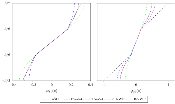
Figure 1: Transverse shear WF of the rectangular $\displaystyle[0/90/0]$ composite plate with $\displaystyle a/h=4$ for each model.

Figure 2: Nondimensionalized transverse shear stresses of the rectangular $\displaystyle[0/90/0]$ composite plate with $\displaystyle a/h=4$ for each model.

a/h

Model

$\displaystyle w^{*}$

%

%

$\displaystyle\sigma_{13}(B)$

%

%

$\displaystyle\sigma_{23}(A)$

%

%

$\displaystyle\omega^{*}$

%

%

2 FoSDT $\displaystyle 6.6164$ $\displaystyle-18.98$ $\displaystyle-21.69$ $\displaystyle 4.2978$ $\displaystyle+67.17$ $\displaystyle+64.28$ $\displaystyle 0.54919$ $\displaystyle-17.76$ $\displaystyle-13.75$ $\displaystyle 3.8633$ $\displaystyle+12.97$ $\displaystyle+13.01$ ToSDT $\displaystyle 7.8944$ $\displaystyle-3.32$ $\displaystyle-6.56$ $\displaystyle 2.4649$ $\displaystyle-4.12$ $\displaystyle-5.78$ $\displaystyle 0.59477$ $\displaystyle-10.93$ $\displaystyle-6.59$ $\displaystyle 3.5335$ $\displaystyle+3.33$ $\displaystyle+3.36$ FoZZ-4 $\displaystyle 7.8130$ $\displaystyle-4.32$ $\displaystyle-7.52$ $\displaystyle 2.0026$ $\displaystyle-22.11$ $\displaystyle-23.45$ $\displaystyle 0.66040$ $\displaystyle-1.11$ $\displaystyle+3.72$ $\displaystyle 3.5485$ $\displaystyle+3.76$ $\displaystyle+3.80$ ToZZ-4 $\displaystyle 6.4960$ $\displaystyle-20.45$ $\displaystyle-23.11$ $\displaystyle 1.4032$ $\displaystyle-45.42$ $\displaystyle-46.36$ $\displaystyle 0.47682$ $\displaystyle-28.60$ $\displaystyle-25.11$ $\displaystyle 3.8845$ $\displaystyle+13.59$ $\displaystyle+13.63$ 3D-WF $\displaystyle 8.4451$ $\displaystyle+3.42$ $\displaystyle-0.04$ $\displaystyle 2.6931$ $\displaystyle+4.76$ $\displaystyle+2.94$ $\displaystyle 0.64111$ $\displaystyle-3.99$ $\displaystyle+0.69$ $\displaystyle 3.4196$ $\displaystyle-0.00$ $\displaystyle+0.03$ Ite-WF $\displaystyle 8.4487$ $\displaystyle+3.46$ $\displaystyle-0.00$ $\displaystyle 2.6163$ $\displaystyle+1.76$ $\displaystyle+0.00$ $\displaystyle 0.63670$ $\displaystyle-4.65$ $\displaystyle+0.00$ $\displaystyle 3.4186$ $\displaystyle-0.03$ $\displaystyle+0.00$ Exa² $\displaystyle 8.4488$ ref. $\displaystyle 2.6162$ ref. $\displaystyle 0.63670$ ref. $\displaystyle 3.4185$ ref. Exa $\displaystyle 8.1659$ ref. $\displaystyle 2.5709$ ref. $\displaystyle 0.66779$ ref. $\displaystyle 3.4197$ ref. 4 FoSDT $\displaystyle 2.0547$ $\displaystyle-27.17$ $\displaystyle-27.80$ $\displaystyle 4.3625$ $\displaystyle+24.26$ $\displaystyle+24.05$ $\displaystyle 0.25631$ $\displaystyle-23.18$ $\displaystyle-18.89$ $\displaystyle 6.9503$ $\displaystyle+17.60$ $\displaystyle+17.64$ ToSDT $\displaystyle 2.6411$ $\displaystyle-6.38$ $\displaystyle-7.20$ $\displaystyle 3.8253$ $\displaystyle+8.96$ $\displaystyle+8.78$ $\displaystyle 0.30414$ $\displaystyle-8.84$ $\displaystyle-3.75$ $\displaystyle 6.1331$ $\displaystyle+3.77$ $\displaystyle+3.80$ FoZZ-4 $\displaystyle 2.7172$ $\displaystyle-3.68$ $\displaystyle-4.52$ $\displaystyle 3.6580$ $\displaystyle+4.19$ $\displaystyle+4.02$ $\displaystyle 0.31797$ $\displaystyle-4.70$ $\displaystyle+0.62$ $\displaystyle 6.0461$ $\displaystyle+2.30$ $\displaystyle+2.33$ ToZZ-4 $\displaystyle 2.7331$ $\displaystyle-3.12$ $\displaystyle-3.96$ $\displaystyle 3.2669$ $\displaystyle-6.95$ $\displaystyle-7.10$ $\displaystyle 0.30071$ $\displaystyle-9.87$ $\displaystyle-4.84$ $\displaystyle 6.0265$ $\displaystyle+1.97$ $\displaystyle+2.00$ 3D-WF $\displaystyle 2.8459$ $\displaystyle+0.88$ $\displaystyle-0.00$ $\displaystyle 3.5182$ $\displaystyle+0.21$ $\displaystyle+0.04$ $\displaystyle 0.31616$ $\displaystyle-5.24$ $\displaystyle+0.05$ $\displaystyle 5.9084$ $\displaystyle-0.03$ $\displaystyle+0.00$ Ite-WF $\displaystyle 2.8459$ $\displaystyle+0.88$ $\displaystyle-0.00$ $\displaystyle 3.5167$ $\displaystyle+0.17$ $\displaystyle+0.00$ $\displaystyle 0.31600$ $\displaystyle-5.29$ $\displaystyle+0.00$ $\displaystyle 5.9084$ $\displaystyle-0.03$ $\displaystyle+0.00$ Exa² $\displaystyle 2.8459$ ref. $\displaystyle 3.5167$ ref. $\displaystyle 0.31600$ ref. $\displaystyle 5.9083$ ref. Exa $\displaystyle 2.8211$ ref. $\displaystyle 3.5108$ ref. $\displaystyle 0.33365$ ref. $\displaystyle 5.9100$ ref. 10 FoSDT $\displaystyle 0.75314$ $\displaystyle-18.04$ $\displaystyle-18.19$ $\displaystyle 4.3895$ $\displaystyle+4.48$ $\displaystyle+4.48$ $\displaystyle 0.13418$ $\displaystyle-11.94$ $\displaystyle-9.77$ $\displaystyle 11.497$ $\displaystyle+10.47$ $\displaystyle+10.49$ ToSDT $\displaystyle 0.86219$ $\displaystyle-6.17$ $\displaystyle-6.34$ $\displaystyle 4.2988$ $\displaystyle+2.32$ $\displaystyle+2.32$ $\displaystyle 0.14468$ $\displaystyle-5.05$ $\displaystyle-2.71$ $\displaystyle 10.750$ $\displaystyle+3.29$ $\displaystyle+3.31$ FoZZ-4 $\displaystyle 0.88102$ $\displaystyle-4.12$ $\displaystyle-4.30$ $\displaystyle 4.2687$ $\displaystyle+1.60$ $\displaystyle+1.61$ $\displaystyle 0.14659$ $\displaystyle-3.80$ $\displaystyle-1.42$ $\displaystyle 10.635$ $\displaystyle+2.19$ $\displaystyle+2.21$ ToZZ-4 $\displaystyle 0.91831$ $\displaystyle-0.07$ $\displaystyle-0.25$ $\displaystyle 4.1841$ $\displaystyle-0.41$ $\displaystyle-0.41$ $\displaystyle 0.14813$ $\displaystyle-2.79$ $\displaystyle-0.39$ $\displaystyle 10.418$ $\displaystyle+0.10$ $\displaystyle+0.12$ 3D-WF $\displaystyle 0.92059$ $\displaystyle+0.18$ $\displaystyle-0.00$ $\displaystyle 4.2011$ $\displaystyle-0.01$ $\displaystyle-0.00$ $\displaystyle 0.14871$ $\displaystyle-2.41$ $\displaystyle+0.00$ $\displaystyle 10.405$ $\displaystyle-0.02$ $\displaystyle+0.00$ Ite-WF $\displaystyle 0.92059$ $\displaystyle+0.18$ $\displaystyle-0.00$ $\displaystyle 4.2012$ $\displaystyle-0.00$ $\displaystyle+0.00$ $\displaystyle 0.14871$ $\displaystyle-2.41$ $\displaystyle+0.00$ $\displaystyle 10.405$ $\displaystyle-0.02$ $\displaystyle+0.00$ Exa² $\displaystyle 0.92059$ ref. $\displaystyle 4.2012$ ref. $\displaystyle 0.14870$ ref. $\displaystyle 10.405$ ref. Exa $\displaystyle 0.91891$ ref. $\displaystyle 4.2014$ ref. $\displaystyle 0.15237$ ref. $\displaystyle 10.408$ ref. 100 FoSDT $\displaystyle 0.50588$ $\displaystyle-0.35$ $\displaystyle-0.35$ $\displaystyle 4.3952$ $\displaystyle+0.05$ $\displaystyle+0.05$ $\displaystyle 0.10816$ $\displaystyle-0.18$ $\displaystyle-0.15$ $\displaystyle 14.059$ $\displaystyle+0.18$ $\displaystyle+0.18$ ToSDT $\displaystyle 0.50700$ $\displaystyle-0.13$ $\displaystyle-0.13$ $\displaystyle 4.3943$ $\displaystyle+0.03$ $\displaystyle+0.03$ $\displaystyle 0.10827$ $\displaystyle-0.08$ $\displaystyle-0.04$ $\displaystyle 14.043$ $\displaystyle+0.07$ $\displaystyle+0.07$ FoZZ-4 $\displaystyle 0.50721$ $\displaystyle-0.09$ $\displaystyle-0.09$ $\displaystyle 4.3940$ $\displaystyle+0.02$ $\displaystyle+0.02$ $\displaystyle 0.10829$ $\displaystyle-0.06$ $\displaystyle-0.03$ $\displaystyle 14.041$ $\displaystyle+0.05$ $\displaystyle+0.05$ ToZZ-4 $\displaystyle 0.50766$ $\displaystyle+0.00$ $\displaystyle-0.00$ $\displaystyle 4.3931$ $\displaystyle-0.00$ $\displaystyle-0.00$ $\displaystyle 0.10832$ $\displaystyle-0.04$ $\displaystyle-0.00$ $\displaystyle 14.034$ $\displaystyle+0.00$ $\displaystyle+0.00$ 3D-WF $\displaystyle 0.50767$ $\displaystyle+0.00$ $\displaystyle-0.00$ $\displaystyle 4.3932$ $\displaystyle-0.00$ $\displaystyle+0.00$ $\displaystyle 0.10832$ $\displaystyle-0.04$ $\displaystyle+0.00$ $\displaystyle 14.034$ $\displaystyle-0.00$ $\displaystyle+0.00$ Ite-WF $\displaystyle 0.50767$ $\displaystyle+0.00$ $\displaystyle-0.00$ $\displaystyle 4.3932$ $\displaystyle-0.00$ $\displaystyle+0.00$ $\displaystyle 0.10832$ $\displaystyle-0.04$ $\displaystyle+0.00$ $\displaystyle 14.034$ $\displaystyle-0.00$ $\displaystyle+0.00$ Exa² $\displaystyle 0.50767$ ref. $\displaystyle 4.3932$ ref. $\displaystyle 0.10832$ ref. $\displaystyle 14.034$ ref. Exa $\displaystyle 0.50766$ ref. $\displaystyle 4.3932$ ref. $\displaystyle 0.10836$ ref. $\displaystyle 14.034$ ref.

Table 2: Comparison between the different models for the rectangular $\displaystyle[0/90/0]$ composite plate with a varying length-to-thickness ratio.

6.2 Square $\displaystyle[0/c/0]$ sandwich plate

In order to study the behavior of a structure exhibiting a high variation of stiffness through the thickness, we propose to study a square sandwich plate with ply thicknesses $\displaystyle h_{1}=h_{3}=0.1h$ and $\displaystyle h_{2}=0.8h$. The face sheets are made of one ply of unidirectional composite and the core is constituted of a honeycomb-type material. Material properties are presented in table 1. Results presented in table 6.2 show that, this time, Reddy’s model (ToSDT) is not as accurate as in the previous case, although Cho’s model (ToZZ-4) obtains better values. This is due to the particular nature of sandwich materials which gives typically zig-zag variations for displacements through the thickness and then typically zig-zag WF. Cho’s model (ToZZ-4) is able to fit this kind of variation although Reddy’s (ToSDT) model is not. The Sun & Withney model (FoZZ-4) has also been proved to be very efficient for sandwiches, which can be verified in this table. Note that the two proposed models, 3D-WF and Ite-WF, globally give the best results. Comparison with the Exa² model is discussed in section 6.6.

Figure 3 shows the corresponding WF for $\displaystyle a/h=4$, for all plate models except the FoSDT one. Figure 4 presents the variations of the transverse shear stresses obtained by integration of the equilibrium equations for all models, compared to the exact solution, in the $\displaystyle a/h=4$ case.

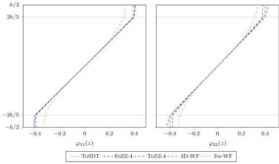
Figure 3: Transverse shear WF of the $\displaystyle[0/c/0]$ sandwich plate with $\displaystyle a/h=4$ for each model.

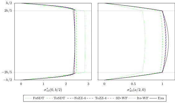
Figure 4: Nondimensionalized transverse shear stresses of the $\displaystyle[0/c/0]$ sandwich plate with $\displaystyle a/h=4$ for each model.

Table 3: Comparison between the different models for the square $\displaystyle[0/c/0]$ sandwich plate with a varying length-to-thickness ratio.

FoSDT $\displaystyle 0.50904$ $\displaystyle-44.74$ $\displaystyle-44.07$ $\displaystyle 2.5177$ $\displaystyle+31.01$ $\displaystyle+35.10$ $\displaystyle 1.0476$ $\displaystyle-30.40$ $\displaystyle-24.36$ $\displaystyle 6.9339$ $\displaystyle+29.88$ $\displaystyle+31.57$ ToSDT $\displaystyle 0.85344$ $\displaystyle-7.34$ $\displaystyle-6.23$ $\displaystyle 1.9150$ $\displaystyle-0.35$ $\displaystyle+2.76$ $\displaystyle 1.3300$ $\displaystyle-11.65$ $\displaystyle-3.97$ $\displaystyle 5.4307$ $\displaystyle+1.72$ $\displaystyle+3.04$ FoZZ-4 $\displaystyle 0.90224$ $\displaystyle-2.05$ $\displaystyle-0.86$ $\displaystyle 1.8459$ $\displaystyle-3.95$ $\displaystyle-0.95$ $\displaystyle 1.3963$ $\displaystyle-7.24$ $\displaystyle+0.82$ $\displaystyle 5.2900$ $\displaystyle-0.92$ $\displaystyle+0.37$ ToZZ-4 $\displaystyle 0.88896$ $\displaystyle-3.49$ $\displaystyle-2.32$ $\displaystyle 1.8320$ $\displaystyle-4.67$ $\displaystyle-1.70$ $\displaystyle 1.3570$ $\displaystyle-9.85$ $\displaystyle-2.02$ $\displaystyle 5.3281$ $\displaystyle-0.20$ $\displaystyle+1.10$ 3D-WF $\displaystyle 0.90894$ $\displaystyle-1.32$ $\displaystyle-0.13$ $\displaystyle 1.8562$ $\displaystyle-3.41$ $\displaystyle-0.40$ $\displaystyle 1.3795$ $\displaystyle-8.36$ $\displaystyle-0.40$ $\displaystyle 5.2730$ $\displaystyle-1.23$ $\displaystyle+0.05$ Ite-WF $\displaystyle 0.91010$ $\displaystyle-1.19$ $\displaystyle-0.00$ $\displaystyle 1.8636$ $\displaystyle-3.02$ $\displaystyle+0.00$ $\displaystyle 1.3850$ $\displaystyle-7.99$ $\displaystyle+0.00$ $\displaystyle 5.2703$ $\displaystyle-1.28$ $\displaystyle+0.00$ Exa² $\displaystyle 0.91010$ ref. $\displaystyle 1.8636$ ref. $\displaystyle 1.3850$ ref. $\displaystyle 5.2702$ ref. Exa $\displaystyle 0.92108$ ref. $\displaystyle 1.9217$ ref. $\displaystyle 1.5053$ ref. $\displaystyle 5.3389$ ref. 4 FoSDT $\displaystyle 0.16645$ $\displaystyle-45.57$ $\displaystyle-45.67$ $\displaystyle 2.8525$ $\displaystyle+18.99$ $\displaystyle+19.09$ $\displaystyle 0.69992$ $\displaystyle-36.72$ $\displaystyle-34.02$ $\displaystyle 12.233$ $\displaystyle+33.77$ $\displaystyle+34.67$ ToSDT $\displaystyle 0.28349$ $\displaystyle-7.30$ $\displaystyle-7.47$ $\displaystyle 2.4657$ $\displaystyle+2.85$ $\displaystyle+2.94$ $\displaystyle 1.0011$ $\displaystyle-9.49$ $\displaystyle-5.63$ $\displaystyle 9.4350$ $\displaystyle+3.17$ $\displaystyle+3.86$ FoZZ-4 $\displaystyle 0.30453$ $\displaystyle-0.42$ $\displaystyle-0.60$ $\displaystyle 2.3971$ $\displaystyle-0.01$ $\displaystyle+0.08$ $\displaystyle 1.0651$ $\displaystyle-3.70$ $\displaystyle+0.41$ $\displaystyle 9.1084$ $\displaystyle-0.40$ $\displaystyle+0.27$ ToZZ-4 $\displaystyle 0.30416$ $\displaystyle-0.54$ $\displaystyle-0.72$ $\displaystyle 2.3897$ $\displaystyle-0.32$ $\displaystyle-0.23$ $\displaystyle 1.0560$ $\displaystyle-4.52$ $\displaystyle-0.45$ $\displaystyle 9.1152$ $\displaystyle-0.33$ $\displaystyle+0.34$ 3D-WF $\displaystyle 0.30636$ $\displaystyle+0.18$ $\displaystyle-0.01$ $\displaystyle 2.3947$ $\displaystyle-0.11$ $\displaystyle-0.02$ $\displaystyle 1.0603$ $\displaystyle-4.13$ $\displaystyle-0.04$ $\displaystyle 9.0843$ $\displaystyle-0.67$ $\displaystyle+0.00$ Ite-WF $\displaystyle 0.30638$ $\displaystyle+0.19$ $\displaystyle-0.00$ $\displaystyle 2.3952$ $\displaystyle-0.09$ $\displaystyle+0.00$ $\displaystyle 1.0607$ $\displaystyle-4.09$ $\displaystyle+0.00$ $\displaystyle 9.0840$ $\displaystyle-0.67$ $\displaystyle+0.00$ Exa² $\displaystyle 0.30638$ ref. $\displaystyle 2.3952$ ref. $\displaystyle 1.0607$ ref. $\displaystyle 9.0840$ ref. Exa $\displaystyle 0.30581$ ref. $\displaystyle 2.3973$ ref. $\displaystyle 1.1060$ ref. $\displaystyle 9.1452$ ref. 10 FoSDT $\displaystyle 0.057970$ $\displaystyle-34.15$ $\displaystyle-34.25$ $\displaystyle 3.1506$ $\displaystyle+5.10$ $\displaystyle+5.00$ $\displaystyle 0.39042$ $\displaystyle-26.89$ $\displaystyle-25.45$ $\displaystyle 21.096$ $\displaystyle+22.82$ $\displaystyle+23.06$ ToSDT $\displaystyle 0.082517$ $\displaystyle-6.27$ $\displaystyle-6.41$ $\displaystyle 3.0293$ $\displaystyle+1.05$ $\displaystyle+0.96$ $\displaystyle 0.49783$ $\displaystyle-6.77$ $\displaystyle-4.95$ $\displaystyle 17.716$ $\displaystyle+3.14$ $\displaystyle+3.35$ FoZZ-4 $\displaystyle 0.087730$ $\displaystyle-0.34$ $\displaystyle-0.50$ $\displaystyle 3.0029$ $\displaystyle+0.17$ $\displaystyle+0.08$ $\displaystyle 0.52287$ $\displaystyle-2.08$ $\displaystyle-0.16$ $\displaystyle 17.185$ $\displaystyle+0.05$ $\displaystyle+0.25$ ToZZ-4 $\displaystyle 0.087908$ $\displaystyle-0.14$ $\displaystyle-0.30$ $\displaystyle 3.0001$ $\displaystyle+0.08$ $\displaystyle-0.01$ $\displaystyle 0.52265$ $\displaystyle-2.12$ $\displaystyle-0.20$ $\displaystyle 17.168$ $\displaystyle-0.05$ $\displaystyle+0.15$ 3D-WF $\displaystyle 0.088171$ $\displaystyle+0.16$ $\displaystyle-0.00$ $\displaystyle 3.0005$ $\displaystyle+0.09$ $\displaystyle-0.00$ $\displaystyle 0.52371$ $\displaystyle-1.93$ $\displaystyle-0.00$ $\displaystyle 17.143$ $\displaystyle-0.20$ $\displaystyle+0.00$ Ite-WF $\displaystyle 0.088172$ $\displaystyle+0.16$ $\displaystyle-0.00$ $\displaystyle 3.0005$ $\displaystyle+0.09$ $\displaystyle+0.00$ $\displaystyle 0.52373$ $\displaystyle-1.92$ $\displaystyle-0.00$ $\displaystyle 17.143$ $\displaystyle-0.20$ $\displaystyle+0.00$ Exa² $\displaystyle 0.088172$ ref. $\displaystyle 3.0005$ ref. $\displaystyle 0.52373$ ref. $\displaystyle 17.143$ ref. Exa $\displaystyle 0.088033$ ref. $\displaystyle 2.9978$ ref. $\displaystyle 0.53399$ ref. $\displaystyle 17.177$ ref. 100 FoSDT $\displaystyle 0.035362$ $\displaystyle-0.93$ $\displaystyle-0.94$ $\displaystyle 3.2418$ $\displaystyle+0.06$ $\displaystyle+0.06$ $\displaystyle 0.29572$ $\displaystyle-0.60$ $\displaystyle-0.56$ $\displaystyle 27.275$ $\displaystyle+0.47$ $\displaystyle+0.47$ ToSDT $\displaystyle 0.035631$ $\displaystyle-0.18$ $\displaystyle-0.18$ $\displaystyle 3.2404$ $\displaystyle+0.01$ $\displaystyle+0.01$ $\displaystyle 0.29705$ $\displaystyle-0.15$ $\displaystyle-0.12$ $\displaystyle 27.172$ $\displaystyle+0.09$ $\displaystyle+0.09$ FoZZ-4 $\displaystyle 0.035691$ $\displaystyle-0.01$ $\displaystyle-0.01$ $\displaystyle 3.2400$ $\displaystyle+0.00$ $\displaystyle+0.00$ $\displaystyle 0.29738$ $\displaystyle-0.05$ $\displaystyle-0.01$ $\displaystyle 27.149$ $\displaystyle+0.00$ $\displaystyle+0.01$ ToZZ-4 $\displaystyle 0.035694$ $\displaystyle-0.00$ $\displaystyle-0.01$ $\displaystyle 3.2400$ $\displaystyle+0.00$ $\displaystyle+0.00$ $\displaystyle 0.29738$ $\displaystyle-0.04$ $\displaystyle-0.00$ $\displaystyle 27.148$ $\displaystyle+0.00$ $\displaystyle+0.00$ 3D-WF $\displaystyle 0.035697$ $\displaystyle+0.00$ $\displaystyle-0.00$ $\displaystyle 3.2400$ $\displaystyle+0.00$ $\displaystyle+0.00$ $\displaystyle 0.29740$ $\displaystyle-0.04$ $\displaystyle-0.00$ $\displaystyle 27.147$ $\displaystyle-0.00$ $\displaystyle-0.00$ Ite-WF $\displaystyle 0.035697$ $\displaystyle+0.00$ $\displaystyle-0.00$ $\displaystyle 3.2400$ $\displaystyle+0.00$ $\displaystyle+0.00$ $\displaystyle 0.29740$ $\displaystyle-0.04$ $\displaystyle-0.00$ $\displaystyle 27.147$ $\displaystyle-0.00$ $\displaystyle-0.00$ Exa² $\displaystyle 0.035697$ ref. $\displaystyle 3.2400$ ref. $\displaystyle 0.29740$ ref. $\displaystyle 27.147$ ref. Exa $\displaystyle 0.035695$ ref. $\displaystyle 3.2399$ ref. $\displaystyle 0.29751$ ref. $\displaystyle 27.148$ ref.

6.3 Square $\displaystyle[-15/15]$ antisymmetric angle-ply composite plate

As the two previous cases enter in the cross-ply family, let us now consider an antisymmetric angle-ply square plate with two layers of equal thickness and a $\displaystyle[-15/15]$ stacking sequence. Transverse stresses $\displaystyle\sigma_{23}(0,b/2,z)$ and $\displaystyle\sigma_{13}(a/2,0,z)$ are no longer null for this laminate but $\displaystyle\sigma_{23}(B)$ and $\displaystyle\sigma_{13}(A)$ are. Hence, these stresses have been computed respectively at points $\displaystyle D(0,b/2,h/4)$ and $\displaystyle C(a/2,0,h/4)$ in order to make comparisons between all models. Results are presented in table 6.1. The tendency of predictions is almost the same than for the $\displaystyle[0/90/0]$ case but it can be noticed that poor values are obtained for the stresses at points D and C. These values are influenced by the way the model is able to couple the $\displaystyle x$ and $\displaystyle y$ direction in the kinematic field, i.e. the presence of non null $\displaystyle\varphi_{12}(z)$ and $\displaystyle\varphi_{21}(z)$ functions. This is only the case for the FoZZ-4, ToZZ-4, 3D-WF and Ite-WF models. However, Cho’s model (ToZZ-4) does not give very good values for the lowest length-to-thickness values, but it was also the case for the $\displaystyle[0/90/0]$ laminate. That suggests that the problem may be due to other causes; this point is discussed later. The two proposed models, 3D-WF and Ite-WF, globally give the best results. However, quite poor estimations of transverse shear stresses are obtained at points C and D in the $\displaystyle a/h=2$ case. Comparison with the Exa² model is let to the section 6.6.

Figure 5 shows the corresponding WF for $\displaystyle a/h=4$, for all plate models except the FoSDT one. Figure 6 presents the variations of the transverse shear stresses obtained by integration of the equilibrium equations for all models, compared to the exact solution, in the $\displaystyle a/h=4$ case.

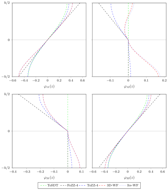
Figure 5: Transverse shear WF of the $\displaystyle[-15/15]$ antisymmetric angle-ply composite plate with $\displaystyle a/h=4$ for each model.

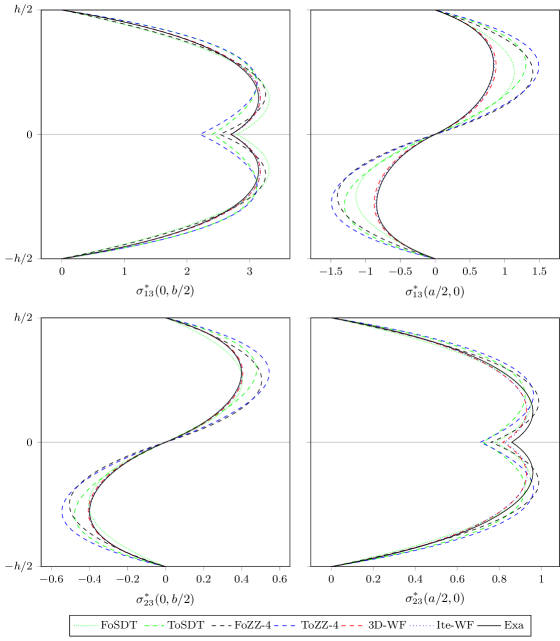
Figure 6: Nondimensionalized transverse shear stresses of the $\displaystyle[-15/15]$ antisymmetric angle-ply composite plate with $\displaystyle a/h=4$ for each model.

6.4 Square $\displaystyle[0]$ single ply composite plate

This square composite plate is made of a single ply oriented at $\displaystyle 0^{\circ}$. For this single layer case, the FoSDT model (without shear correction factors) and the FoZZ-4 exactly coincides. It is also the case for Reddy’s and Cho’s models (ToSDT and ToZZ-4). Note that the $\displaystyle x$ and $\displaystyle y$ directions are not equivalent for the considered laminate, but for Cho’s model in this case, $\displaystyle\varphi_{11}(z)=\varphi_{22}(z)$. This is not true for 3D-WF and Ite-WF models which exhibits different $\displaystyle\varphi_{11}(z)$ and $\displaystyle\varphi_{22}(z)$ functions due to the different longitudinal/shear modulus ratios in each direction. Note also that, even if it has not been presented in this paper, the WF for these two models depend on the length-to-thickness ratio. The proposed models, 3D-WF and Ite-WF, give poorer values for the deflection than those of the ToSDT model. However, the stresses and the fundamental frequency are best predicted. As we shall see later in section 6.6, the plane stress hypothesis is no longer valid for such low length-to-thickness ratios, that is the reason why the Exa² solution has been introduced.

Figure 7 shows the corresponding WF for $\displaystyle a/h=4$, for all plate models except the FoSDT one. Figure 8 presents the variations of the transverse shear stresses obtained by integration of the equilibrium equations for all models, compared to the exact solution, in the $\displaystyle a/h=4$ case.

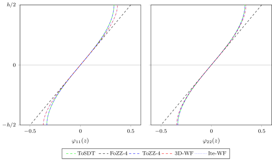
Figure 7: Transverse shear WF of the $\displaystyle[0]$ single ply composite plate with $\displaystyle a/h=4$ for each model.

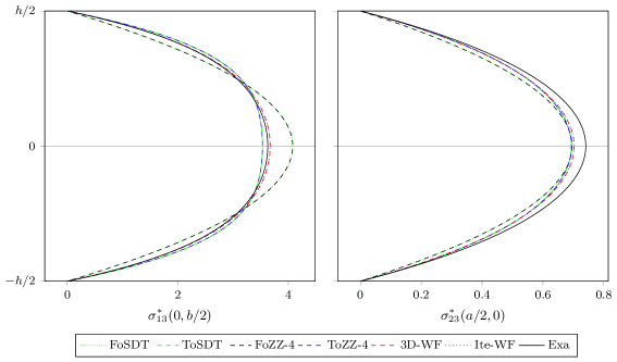
Figure 8: Nondimensionalized transverse shear stresses of the $\displaystyle[0]$ single ply composite plate with $\displaystyle a/h=4$ for each model.

Table 4: Comparison between the different models for the square $\displaystyle[0]$ single ply composite plate with a varying length-to-thickness ratio.

FoSDT $\displaystyle 4.3108$ $\displaystyle-3.63$ $\displaystyle-9.94$ $\displaystyle 3.7502$ $\displaystyle+31.36$ $\displaystyle+24.72$ $\displaystyle 1.0244$ $\displaystyle+2.65$ $\displaystyle+8.26$ $\displaystyle 4.7281$ $\displaystyle+4.85$ $\displaystyle+5.05$ ToSDT $\displaystyle 4.5262$ $\displaystyle+1.19$ $\displaystyle-5.44$ $\displaystyle 2.0291$ $\displaystyle-28.93$ $\displaystyle-32.52$ $\displaystyle 0.85739$ $\displaystyle-14.09$ $\displaystyle-9.39$ $\displaystyle 4.6223$ $\displaystyle+2.50$ $\displaystyle+2.70$ FoZZ-4 $\displaystyle 4.3108$ $\displaystyle-3.63$ $\displaystyle-9.94$ $\displaystyle 3.7502$ $\displaystyle+31.36$ $\displaystyle+24.72$ $\displaystyle 1.0244$ $\displaystyle+2.65$ $\displaystyle+8.26$ $\displaystyle 4.7281$ $\displaystyle+4.85$ $\displaystyle+5.05$ ToZZ-4 $\displaystyle 4.5262$ $\displaystyle+1.19$ $\displaystyle-5.44$ $\displaystyle 2.0291$ $\displaystyle-28.93$ $\displaystyle-32.52$ $\displaystyle 0.85739$ $\displaystyle-14.09$ $\displaystyle-9.39$ $\displaystyle 4.6223$ $\displaystyle+2.50$ $\displaystyle+2.70$ 3D-WF $\displaystyle 4.7804$ $\displaystyle+6.87$ $\displaystyle-0.13$ $\displaystyle 3.1758$ $\displaystyle+11.24$ $\displaystyle+5.62$ $\displaystyle 0.95157$ $\displaystyle-4.65$ $\displaystyle+0.56$ $\displaystyle 4.5040$ $\displaystyle-0.12$ $\displaystyle+0.07$ Ite-WF $\displaystyle 4.7861$ $\displaystyle+7.00$ $\displaystyle-0.01$ $\displaystyle 3.0077$ $\displaystyle+5.35$ $\displaystyle+0.03$ $\displaystyle 0.94628$ $\displaystyle-5.18$ $\displaystyle+0.00$ $\displaystyle 4.5009$ $\displaystyle-0.19$ $\displaystyle+0.00$ Exa² $\displaystyle 4.7864$ ref. $\displaystyle 3.0069$ ref. $\displaystyle 0.94624$ ref. $\displaystyle 4.5007$ ref. Exa $\displaystyle 4.4730$ ref. $\displaystyle 2.8549$ ref. $\displaystyle 0.99796$ ref. $\displaystyle 4.5093$ ref. 4 FoSDT $\displaystyle 1.4643$ $\displaystyle-8.42$ $\displaystyle-10.16$ $\displaystyle 4.0792$ $\displaystyle+12.44$ $\displaystyle+11.18$ $\displaystyle 0.69540$ $\displaystyle-6.14$ $\displaystyle-0.98$ $\displaystyle 8.1438$ $\displaystyle+5.17$ $\displaystyle+5.34$ ToSDT $\displaystyle 1.6206$ $\displaystyle+1.35$ $\displaystyle-0.57$ $\displaystyle 3.5324$ $\displaystyle-2.63$ $\displaystyle-3.72$ $\displaystyle 0.69382$ $\displaystyle-6.35$ $\displaystyle-1.21$ $\displaystyle 7.7522$ $\displaystyle+0.11$ $\displaystyle+0.28$ FoZZ-4 $\displaystyle 1.4643$ $\displaystyle-8.42$ $\displaystyle-10.16$ $\displaystyle 4.0792$ $\displaystyle+12.44$ $\displaystyle+11.18$ $\displaystyle 0.69540$ $\displaystyle-6.14$ $\displaystyle-0.98$ $\displaystyle 8.1438$ $\displaystyle+5.17$ $\displaystyle+5.34$ ToZZ-4 $\displaystyle 1.6206$ $\displaystyle+1.35$ $\displaystyle-0.57$ $\displaystyle 3.5324$ $\displaystyle-2.63$ $\displaystyle-3.72$ $\displaystyle 0.69382$ $\displaystyle-6.35$ $\displaystyle-1.21$ $\displaystyle 7.7522$ $\displaystyle+0.11$ $\displaystyle+0.28$ 3D-WF $\displaystyle 1.6298$ $\displaystyle+1.93$ $\displaystyle-0.00$ $\displaystyle 3.6718$ $\displaystyle+1.21$ $\displaystyle+0.08$ $\displaystyle 0.70227$ $\displaystyle-5.21$ $\displaystyle-0.00$ $\displaystyle 7.7311$ $\displaystyle-0.16$ $\displaystyle+0.00$ Ite-WF $\displaystyle 1.6298$ $\displaystyle+1.93$ $\displaystyle-0.00$ $\displaystyle 3.6693$ $\displaystyle+1.14$ $\displaystyle+0.01$ $\displaystyle 0.70231$ $\displaystyle-5.21$ $\displaystyle+0.00$ $\displaystyle 7.7311$ $\displaystyle-0.16$ $\displaystyle+0.00$ Exa² $\displaystyle 1.6299$ ref. $\displaystyle 3.6690$ ref. $\displaystyle 0.70231$ ref. $\displaystyle 7.7310$ ref. Exa $\displaystyle 1.5989$ ref. $\displaystyle 3.6280$ ref. $\displaystyle 0.74089$ ref. $\displaystyle 7.7436$ ref. 10 FoSDT $\displaystyle 0.60418$ $\displaystyle-4.82$ $\displaystyle-5.17$ $\displaystyle 4.3281$ $\displaystyle+2.50$ $\displaystyle+2.32$ $\displaystyle 0.44658$ $\displaystyle-3.85$ $\displaystyle-1.85$ $\displaystyle 12.795$ $\displaystyle+2.59$ $\displaystyle+2.66$ ToSDT $\displaystyle 0.63709$ $\displaystyle+0.37$ $\displaystyle-0.01$ $\displaystyle 4.2249$ $\displaystyle+0.06$ $\displaystyle-0.12$ $\displaystyle 0.45479$ $\displaystyle-2.08$ $\displaystyle-0.05$ $\displaystyle 12.464$ $\displaystyle-0.06$ $\displaystyle+0.00$ FoZZ-4 $\displaystyle 0.60418$ $\displaystyle-4.82$ $\displaystyle-5.17$ $\displaystyle 4.3281$ $\displaystyle+2.50$ $\displaystyle+2.32$ $\displaystyle 0.44658$ $\displaystyle-3.85$ $\displaystyle-1.85$ $\displaystyle 12.795$ $\displaystyle+2.59$ $\displaystyle+2.66$ ToZZ-4 $\displaystyle 0.63709$ $\displaystyle+0.37$ $\displaystyle-0.01$ $\displaystyle 4.2249$ $\displaystyle+0.06$ $\displaystyle-0.12$ $\displaystyle 0.45479$ $\displaystyle-2.08$ $\displaystyle-0.05$ $\displaystyle 12.464$ $\displaystyle-0.06$ $\displaystyle+0.00$ 3D-WF $\displaystyle 0.63714$ $\displaystyle+0.37$ $\displaystyle-0.00$ $\displaystyle 4.2300$ $\displaystyle+0.18$ $\displaystyle-0.00$ $\displaystyle 0.45499$ $\displaystyle-2.03$ $\displaystyle-0.00$ $\displaystyle 12.463$ $\displaystyle-0.06$ $\displaystyle+0.00$ Ite-WF $\displaystyle 0.63714$ $\displaystyle+0.37$ $\displaystyle-0.00$ $\displaystyle 4.2301$ $\displaystyle+0.18$ $\displaystyle+0.00$ $\displaystyle 0.45500$ $\displaystyle-2.03$ $\displaystyle-0.00$ $\displaystyle 12.463$ $\displaystyle-0.06$ $\displaystyle+0.00$ Exa² $\displaystyle 0.63715$ ref. $\displaystyle 4.2300$ ref. $\displaystyle 0.45500$ ref. $\displaystyle 12.463$ ref. Exa $\displaystyle 0.63477$ ref. $\displaystyle 4.2223$ ref. $\displaystyle 0.46444$ ref. $\displaystyle 12.471$ ref. 100 FoSDT $\displaystyle 0.43300$ $\displaystyle-0.08$ $\displaystyle-0.08$ $\displaystyle 4.3973$ $\displaystyle+0.03$ $\displaystyle+0.02$ $\displaystyle 0.37735$ $\displaystyle-0.06$ $\displaystyle-0.03$ $\displaystyle 15.196$ $\displaystyle+0.04$ $\displaystyle+0.04$ ToSDT $\displaystyle 0.43335$ $\displaystyle+0.00$ $\displaystyle-0.00$ $\displaystyle 4.3962$ $\displaystyle+0.00$ $\displaystyle-0.00$ $\displaystyle 0.37746$ $\displaystyle-0.03$ $\displaystyle-0.00$ $\displaystyle 15.190$ $\displaystyle-0.00$ $\displaystyle-0.00$ FoZZ-4 $\displaystyle 0.43300$ $\displaystyle-0.08$ $\displaystyle-0.08$ $\displaystyle 4.3973$ $\displaystyle+0.03$ $\displaystyle+0.02$ $\displaystyle 0.37735$ $\displaystyle-0.06$ $\displaystyle-0.03$ $\displaystyle 15.196$ $\displaystyle+0.04$ $\displaystyle+0.04$ ToZZ-4 $\displaystyle 0.43335$ $\displaystyle+0.00$ $\displaystyle-0.00$ $\displaystyle 4.3962$ $\displaystyle+0.00$ $\displaystyle-0.00$ $\displaystyle 0.37746$ $\displaystyle-0.03$ $\displaystyle-0.00$ $\displaystyle 15.190$ $\displaystyle-0.00$ $\displaystyle-0.00$ 3D-WF $\displaystyle 0.43335$ $\displaystyle+0.00$ $\displaystyle-0.00$ $\displaystyle 4.3962$ $\displaystyle+0.00$ $\displaystyle+0.00$ $\displaystyle 0.37746$ $\displaystyle-0.03$ $\displaystyle-0.00$ $\displaystyle 15.190$ $\displaystyle-0.00$ $\displaystyle+0.00$ Ite-WF $\displaystyle 0.43335$ $\displaystyle+0.00$ $\displaystyle-0.00$ $\displaystyle 4.3962$ $\displaystyle+0.00$ $\displaystyle+0.00$ $\displaystyle 0.37746$ $\displaystyle-0.03$ $\displaystyle-0.00$ $\displaystyle 15.190$ $\displaystyle-0.00$ $\displaystyle+0.00$ Exa² $\displaystyle 0.43335$ ref. $\displaystyle 4.3962$ ref. $\displaystyle 0.37746$ ref. $\displaystyle 15.190$ ref. Exa $\displaystyle 0.43333$ ref. $\displaystyle 4.3961$ ref. $\displaystyle 0.37756$ ref. $\displaystyle 15.190$ ref.

6.5 Square $\displaystyle[0/30/0]$ composite plate

Let us now consider a symmetric angle-ply square plate with three layer of equal thickness and a $\displaystyle[0/30/0]$ stacking sequence. This configuration is chosen since it doesn’t involve any simplification in the linear system (20), i. e. the $\displaystyle[\mathbf{K}]$ matrix doesn’t have any null coefficient. Although this laminate does not represent the more general case (because of its symmetry) it involves an additional $\displaystyle\overline{q}^{mn}\cos(\xi x)\cos(\eta y)$ term in the loading to fulfill the simply supported condition. In other words, it is the only laminate considered in this study which requires a (non-null) Lagrange multiplier in the solving process presented in section 4. Results presented in table 6.1 show the same tendency than for the $\displaystyle[0]$ laminate, which in fact is not so different. Present models, 3D-WF and Ite-WF, give globally better stresses and fundamental frequency, and a poorer deflection, compared to ToSDT or ToZZ-4 model when the Exa solution is taken as reference.

Figure 9 shows the corresponding WF for $\displaystyle a/h=4$, for all plate models except the FoSDT one. Figure 10 presents the variations of the transverse shear stresses obtained by integration of the equilibrium equations for all models, compared to the exact solution, in the $\displaystyle a/h=4$ case.

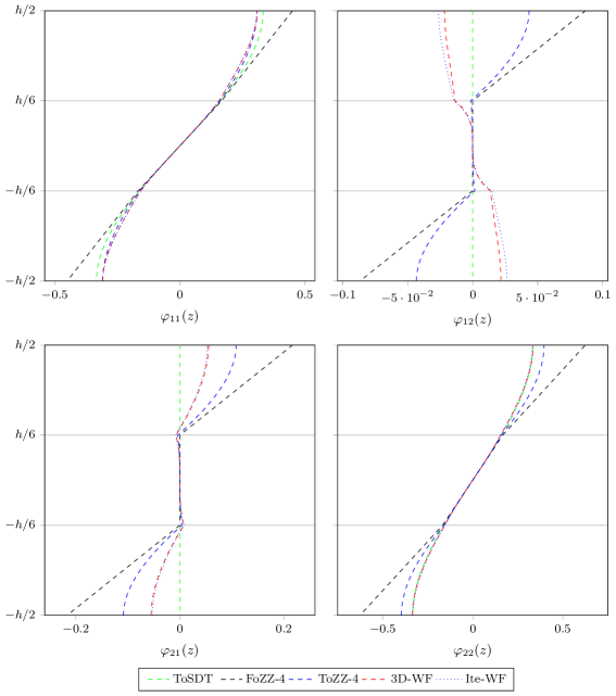
Figure 9: Transverse shear WF of the $\displaystyle[0/30/0]$ composite plate with $\displaystyle a/h=4$ for each model.

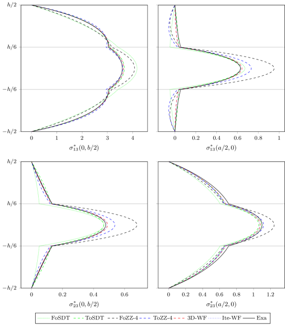
Figure 10: Nondimensionalized transverse shear stresses of the $\displaystyle[0/30/0]$ composite plate with $\displaystyle a/h=4$ for each model.

6.6 Discussion

The five studied cases have been chosen in order to represent a wide range of the laminates diversity. In addition to particular comments done for each case, general results may be issued from these studies. We first compare all models with the Exa analytical solution. The Mindlin model (FoSDT), without the help of appropriate shear correction factors, gives relatively poor values, except for thin plates. For moderately thick plates, Reddy’s model (ToSDT) is very accurate, except for the sandwich case because the high modulus ratio between layers is not properly managed by the model. On the contrary, the Sun & Whitney zig-zag linear model (FoZZ-4) can manage it but fails for classical laminates, especially the single ply. Cho’s model (ToZZ-4) which a priori takes both advantage of a cubic variation coupled to a zig-zag variation of displacements sometimes gives poor values, especially for thick or very-thick plates. These poor estimations are probably due to the fact that the WF of the ToZZ-4 model are too constrained by their formulation: as the cubic term is unique for all the layers, the WF sometimes adopt shapes that are not pertinent. In addition, its WF do not depend on the length-to-thickness ratio. Both proposed models, 3D-WF and Ite-WF, give globally better results in all studied cases than other models. However, some values of the deflection are no so good compared to simpler models. These unexpected results have led to an examination of what was going wrong, and finally to the proposal of the Exa² solution, presented in section 5.1.2. The nature and purpose of this Exa² solution, and the way to obtain it, are there explained.

The comparison for all models can now be done taking the Exa² exact solution as reference. It clearly shows that both proposed 3D-WF and Ite-WF models surpass all other models, giving values for deflection and transverse stresses very close to those of the exact solution, for all studied cases, and for all length to-thickness ratios. The Ite-WF model gives the best results. Of course these spectacular results have to be replaced in the special context of this study. Plate problems solved in this study are simply supported problems with double-sine loading. The WF used for the 3D-WF and Ite-WF model are obtained considering this special bending problem. Results show that the generic model is able to manage all lamination schemes if appropriate WF are provided, but there is no guarantee that the WF obtained for this special bending configuration will work as well as for other configurations. The model with these WF may be a good candidate for other configurations, compared to simpler models, but other WF could perhaps be considered. Further studies need to be done in order to validate –or adapt– the WF to other configurations.

For fundamental frequencies, for both 3D-WF and Ite-WF models, the WF of the static case have been used. This means that the analytical solution used to obtain the WF for the 3D-WF model is obtained with $\displaystyle\omega=0$. This $\displaystyle\omega=0$ condition is also used when the successive equilibrium equations are integrated for the Ite-WF model. Although it is possible, without any additional effort, to set in those processes $\displaystyle\omega$ to the appropriate value (given for example by the Exa solution), it has not be done. This seems to have little effect on the WF for frequency values near the fundamental frequency. This can be seen on their shapes (not presented here) and is corroborated by the satisfactory results for fundamental frequencies given in tables. However, one may think that for higher frequencies the WF need to be modified. Hence further studies have to be done with emphasis for the dynamic behavior.

7 Conclusion

In this paper, a multilayered equivalent-single-layer plate theory based on warping functions (WF) has been presented. Two ways to generate the WF from three dimensional elasticity equations are described. The first one, leading to the 3D-WF model, derives directly the WF from a 3D exact solution, called Exa. The second one, leading to the Ite-WF model, is an iterative process involving successive integrations of the equilibrium equations. Both processes use the same core procedure which issues the WF from the variations of transverse shear stresses. Needed variations of the shear stresses are computed at the middle of the edges of the plate, for a simply supported bending problem with a double-sine loading.

These two models are compared to other models and to the exact solution for five lamination sequences. Considered laminated plates are: a $\displaystyle[0/90/0]$ cross-ply rectangular plate, a square $\displaystyle[0/c/0]$ sandwich plate, a square $\displaystyle[0]$ single layer plate, a square $\displaystyle[-15/15]$ antisymmetric angle-ply plate, and a square plate with a more general $\displaystyle[0/30/0]$ lamination sequence. Models for comparison include Mindlin (FoSDT), Reddy (ToSDT), Sun & Whitney–Woodcock (FoZZ-4), and Kim-Cho (ToZZ-4) models. They have been formulated in terms of WF, so the solution procedure is unique. The problem which is solved for comparison is the simply supported plate with a double-sine loading, for which exact solutions are known. The comparisons are made on deflections, stresses, and fundamental frequencies for length-to-thickness ratios varying from $\displaystyle 2$ to $\displaystyle 100$. The Mindlin (FoSDT) and Reddy (ToSDT) models are not material-dependent, in other words, their WF are unique. In addition, $\displaystyle\varphi_{11}(z)=\varphi_{22}(z)$ and they never have non-null $\displaystyle\varphi_{12}(z)$ or $\displaystyle\varphi_{21}(z)$ WF. All other considered models have WF which depend on material properties and on the lamination sequence, hence have $\displaystyle 4$ different WF for general lamination sequences. In addition, the WF of the 3D-WF and Ite-WF models depend on the length-to-thickness ratio.

Results show that for classical laminates – with moderate modulus ratio between layers – Reddy’s model (ToSDT), which has cubic WF, is a good choice for thin and moderately thick plates, but is not so accurate for sandwich structures. On the contrary, the Sun & Whitney–Woodcock model (FoZZ-4), which has 4 linear zig-zag WF, is a good choice for the sandwich structure but is not accurate enough for classical laminates. Kim-Cho’s model (ToZZ-4), which combines advantages from the two previous models, has 4 cubic zig-zag WF. Its results are then better than those of the previous models when we look at all the classes of laminates. However, Kim-Cho’s model sometimes gives poor results for low length-to-thickness values, probably because the WF are too constrained by their formulation. Comparisons also show that the two presented models, 3D-WF and Ite-WF, give globally better results than other tested models for all considered lamination sequences.

For the thick plates ($\displaystyle a/h\leq 4$), none of the models can be considered as accurate, even if the 3D-WF and Ite-WF models give better values on stresses and fundamental frequencies than other models. As all presented models consider the generalized plane stress hypothesis, an exact plane-stress solution called Exa² has been computed for all considered laminates, in order to make further comparisons. This has been done using the same 3D solution procedure after replacing stiffnesses of all materials with corresponding plane stress stiffnesses. Comparison with the Exa² reference clearly shows that the 3D-WF and Ite-WF models give better results than other models. It can be seen that the Ite-WF model gives nearly exact values of deflection, stresses and fundamental frequencies, for all laminates and for all length-to-thickness ratio values.

These last results show clearly that the comparison of considered models with the Exa exact solution for low length-to-thickness values have no sense because these models do not take into account the transverse deformation and use the generalized plane stress hypothesis. This fact has to be related to the notion of consistency as mentioned in the introduction. From another point of view, all these models try –with more or less success– to simulate another solution which is here denoted Exa². Hence, comparison of considered models with the Exa solution will led to erroneous conclusions on the ability of these models to integrate the transverse shear behavior. As a result, the transverse deformation must be considered if thick plates have to be studied with equivalent-single-layer theories. It might also be the case for laminates which have high stiffness ratios between layers, and for dynamic studies when the wavelength shortens.

Results also show that the generation of WF from an analytical solution or from the integration of equilibrium equations is a relatively easy way to have a very accurate universal model, at least for reasonable length-to-thickness ratios. Further studies must try to establish if the WF obtained by these methods are also pertinent for problems involving other boundary conditions, loading, or frequencies. If it is not the case, other ways to compute pertinent WF have to be investigated. FoSDT $\displaystyle 4.3448$ $\displaystyle-4.61$ $\displaystyle-10.46$ $\displaystyle 2.5852$ $\displaystyle+10.45$ $\displaystyle+9.02$ $\displaystyle 0.96150$ $\displaystyle-8.99$ $\displaystyle-4.02$ $\displaystyle 0.39006$ $\displaystyle+6.66$ $\displaystyle+2.00$ $\displaystyle 1.2538$ $\displaystyle+132.50$ $\displaystyle+103.37$ $\displaystyle 4.7206$ $\displaystyle+5.62$ $\displaystyle+5.70$ ToSDT $\displaystyle 4.3111$ $\displaystyle-5.35$ $\displaystyle-11.15$ $\displaystyle 1.2945$ $\displaystyle-44.70$ $\displaystyle-45.41$ $\displaystyle 0.66314$ $\displaystyle-37.23$ $\displaystyle-33.80$ $\displaystyle 0.61086$ $\displaystyle+67.03$ $\displaystyle+59.73$ $\displaystyle 1.7362$ $\displaystyle+221.94$ $\displaystyle+181.61$ $\displaystyle 4.7611$ $\displaystyle+6.52$ $\displaystyle+6.61$ FoZZ-4 $\displaystyle 3.8609$ $\displaystyle-15.24$ $\displaystyle-20.43$ $\displaystyle 1.5621$ $\displaystyle-33.26$ $\displaystyle-34.13$ $\displaystyle 0.82808$ $\displaystyle-21.62$ $\displaystyle-17.34$ $\displaystyle 0.77361$ $\displaystyle+111.53$ $\displaystyle+102.29$ $\displaystyle 2.3751$ $\displaystyle+340.42$ $\displaystyle+285.24$ $\displaystyle 4.9993$ $\displaystyle+11.85$ $\displaystyle+11.94$ ToZZ-4 $\displaystyle 3.9838$ $\displaystyle-12.54$ $\displaystyle-17.90$ $\displaystyle 0.68465$ $\displaystyle-70.75$ $\displaystyle-71.13$ $\displaystyle 0.58472$ $\displaystyle-44.65$ $\displaystyle-41.63$ $\displaystyle 0.85309$ $\displaystyle+133.26$ $\displaystyle+123.07$ $\displaystyle 2.4671$ $\displaystyle+357.48$ $\displaystyle+300.16$ $\displaystyle 4.9478$ $\displaystyle+10.70$ $\displaystyle+10.79$ 3D-WF $\displaystyle 4.8406$ $\displaystyle+6.28$ $\displaystyle-0.24$ $\displaystyle 2.3183$ $\displaystyle-0.96$ $\displaystyle-2.24$ $\displaystyle 0.93896$ $\displaystyle-11.12$ $\displaystyle-6.27$ $\displaystyle 0.41381$ $\displaystyle+13.15$ $\displaystyle+8.21$ $\displaystyle 0.85886$ $\displaystyle+59.26$ $\displaystyle+39.31$ $\displaystyle 4.4826$ $\displaystyle+0.29$ $\displaystyle+0.37$ Ite-WF $\displaystyle 4.8523$ $\displaystyle+6.53$ $\displaystyle-0.00$ $\displaystyle 2.3720$ $\displaystyle+1.34$ $\displaystyle+0.03$ $\displaystyle 1.0020$ $\displaystyle-5.15$ $\displaystyle+0.03$ $\displaystyle 0.38223$ $\displaystyle+4.51$ $\displaystyle-0.05$ $\displaystyle 0.61566$ $\displaystyle+14.16$ $\displaystyle-0.14$ $\displaystyle 4.4706$ $\displaystyle+0.03$ $\displaystyle+0.10$ Exa² $\displaystyle 4.8524$ ref. $\displaystyle 2.3713$ ref. $\displaystyle 1.0018$ ref. $\displaystyle 0.38243$ ref. $\displaystyle 0.61652$ ref. $\displaystyle 4.4660$ ref. Exa $\displaystyle 4.5548$ ref. $\displaystyle 2.3407$ ref. $\displaystyle 1.0565$ ref. $\displaystyle 0.36572$ ref. $\displaystyle 0.53928$ ref. $\displaystyle 4.4695$ ref. 4 FoSDT $\displaystyle 1.5762$ $\displaystyle-7.60$ $\displaystyle-9.49$ $\displaystyle 2.7968$ $\displaystyle+3.47$ $\displaystyle+3.29$ $\displaystyle 0.77953$ $\displaystyle-9.30$ $\displaystyle-5.53$ $\displaystyle 0.40374$ $\displaystyle+2.37$ $\displaystyle+1.35$ $\displaystyle 1.1382$ $\displaystyle+36.90$ $\displaystyle+34.50$ $\displaystyle 7.7953$ $\displaystyle+4.57$ $\displaystyle+4.88$ ToSDT $\displaystyle 1.6594$ $\displaystyle-2.73$ $\displaystyle-4.72$ $\displaystyle 2.4047$ $\displaystyle-11.04$ $\displaystyle-11.19$ $\displaystyle 0.72164$ $\displaystyle-16.03$ $\displaystyle-12.55$ $\displaystyle 0.46519$ $\displaystyle+17.96$ $\displaystyle+16.78$ $\displaystyle 1.2815$ $\displaystyle+54.14$ $\displaystyle+51.43$ $\displaystyle 7.6323$ $\displaystyle+2.38$ $\displaystyle+2.69$ FoZZ-4 $\displaystyle 1.5082$ $\displaystyle-11.59$ $\displaystyle-13.40$ $\displaystyle 2.5237$ $\displaystyle-6.63$ $\displaystyle-6.79$ $\displaystyle 0.76061$ $\displaystyle-11.50$ $\displaystyle-7.83$ $\displaystyle 0.50488$ $\displaystyle+28.02$ $\displaystyle+26.74$ $\displaystyle 1.4053$ $\displaystyle+69.03$ $\displaystyle+66.06$ $\displaystyle 7.9690$ $\displaystyle+6.90$ $\displaystyle+7.22$ ToZZ-4 $\displaystyle 1.6197$ $\displaystyle-5.05$ $\displaystyle-7.00$ $\displaystyle 2.2063$ $\displaystyle-18.38$ $\displaystyle-18.52$ $\displaystyle 0.70919$ $\displaystyle-17.48$ $\displaystyle-14.06$ $\displaystyle 0.53761$ $\displaystyle+36.32$ $\displaystyle+34.96$ $\displaystyle 1.4786$ $\displaystyle+77.85$ $\displaystyle+74.72$ $\displaystyle 7.7273$ $\displaystyle+3.66$ $\displaystyle+3.97$ 3D-WF $\displaystyle 1.7414$ $\displaystyle+2.08$ $\displaystyle-0.01$ $\displaystyle 2.6980$ $\displaystyle-0.19$ $\displaystyle-0.36$ $\displaystyle 0.81709$ $\displaystyle-4.93$ $\displaystyle-0.98$ $\displaystyle 0.40205$ $\displaystyle+1.95$ $\displaystyle+0.93$ $\displaystyle 0.86867$ $\displaystyle+4.48$ $\displaystyle+2.65$ $\displaystyle 7.4376$ $\displaystyle-0.23$ $\displaystyle+0.07$ Ite-WF $\displaystyle 1.7416$ $\displaystyle+2.09$ $\displaystyle-0.00$ $\displaystyle 2.7078$ $\displaystyle+0.17$ $\displaystyle+0.00$ $\displaystyle 0.82521$ $\displaystyle-3.98$ $\displaystyle+0.00$ $\displaystyle 0.39835$ $\displaystyle+1.01$ $\displaystyle-0.00$ $\displaystyle 0.84627$ $\displaystyle+1.79$ $\displaystyle-0.00$ $\displaystyle 7.4354$ $\displaystyle-0.26$ $\displaystyle+0.04$ Exa² $\displaystyle 1.7416$ ref. $\displaystyle 2.7077$ ref. $\displaystyle 0.82520$ ref. $\displaystyle 0.39836$ ref. $\displaystyle 0.84627$ ref. $\displaystyle 7.4324$ ref. Exa $\displaystyle 1.7059$ ref. $\displaystyle 2.7031$ ref. $\displaystyle 0.85945$ ref. $\displaystyle 0.39437$ ref. $\displaystyle 0.83139$ ref. $\displaystyle 7.4548$ ref. 10 FoSDT $\displaystyle 0.77629$ $\displaystyle-3.29$ $\displaystyle-3.77$ $\displaystyle 2.9520$ $\displaystyle+0.67$ $\displaystyle+0.62$ $\displaystyle 0.64607$ $\displaystyle-3.11$ $\displaystyle-1.97$ $\displaystyle 0.41376$ $\displaystyle+0.54$ $\displaystyle+0.38$ $\displaystyle 1.0534$ $\displaystyle+6.32$ $\displaystyle+6.18$ $\displaystyle 11.218$ $\displaystyle+1.74$ $\displaystyle+1.87$ ToSDT $\displaystyle 0.79522$ $\displaystyle-0.93$ $\displaystyle-1.42$ $\displaystyle 2.8811$ $\displaystyle-1.74$ $\displaystyle-1.79$ $\displaystyle 0.64072$ $\displaystyle-3.92$ $\displaystyle-2.79$ $\displaystyle 0.42393$ $\displaystyle+3.02$ $\displaystyle+2.85$ $\displaystyle 1.0791$ $\displaystyle+8.92$ $\displaystyle+8.77$ $\displaystyle 11.093$ $\displaystyle+0.60$ $\displaystyle+0.73$ FoZZ-4 $\displaystyle 0.76841$ $\displaystyle-4.27$ $\displaystyle-4.75$ $\displaystyle 2.9075$ $\displaystyle-0.84$ $\displaystyle-0.89$ $\displaystyle 0.64468$ $\displaystyle-3.32$ $\displaystyle-2.18$ $\displaystyle 0.43019$ $\displaystyle+4.54$ $\displaystyle+4.36$ $\displaystyle 1.0933$ $\displaystyle+10.34$ $\displaystyle+10.19$ $\displaystyle 11.275$ $\displaystyle+2.26$ $\displaystyle+2.39$ ToZZ-4 $\displaystyle 0.79198$ $\displaystyle-1.34$ $\displaystyle-1.82$ $\displaystyle 2.8463$ $\displaystyle-2.93$ $\displaystyle-2.98$ $\displaystyle 0.64029$ $\displaystyle-3.98$ $\displaystyle-2.85$ $\displaystyle 0.43619$ $\displaystyle+6.00$ $\displaystyle+5.82$ $\displaystyle 1.1098$ $\displaystyle+12.01$ $\displaystyle+11.86$ $\displaystyle 11.116$ $\displaystyle+0.81$ $\displaystyle+0.94$ 3D-WF $\displaystyle 0.80669$ $\displaystyle+0.49$ $\displaystyle-0.00$ $\displaystyle 2.9334$ $\displaystyle+0.04$ $\displaystyle-0.01$ $\displaystyle 0.65877$ $\displaystyle-1.21$ $\displaystyle-0.05$ $\displaystyle 0.41233$ $\displaystyle+0.20$ $\displaystyle+0.03$ $\displaystyle 0.99287$ $\displaystyle+0.21$ $\displaystyle+0.07$ $\displaystyle 11.012$ $\displaystyle-0.13$ $\displaystyle+0.00$ Ite-WF $\displaystyle 0.80669$ $\displaystyle+0.49$ $\displaystyle-0.00$ $\displaystyle 2.9337$ $\displaystyle+0.05$ $\displaystyle+0.00$ $\displaystyle 0.65908$ $\displaystyle-1.16$ $\displaystyle-0.00$ $\displaystyle 0.41220$ $\displaystyle+0.17$ $\displaystyle+0.00$ $\displaystyle 0.99215$ $\displaystyle+0.13$ $\displaystyle+0.00$ $\displaystyle 11.012$ $\displaystyle-0.13$ $\displaystyle+0.00$ Exa² $\displaystyle 0.80669$ ref. $\displaystyle 2.9337$ ref. $\displaystyle 0.65908$ ref. $\displaystyle 0.41220$ ref. $\displaystyle 0.99214$ ref. $\displaystyle 11.012$ ref. Exa $\displaystyle 0.80272$ ref. $\displaystyle 2.9323$ ref. $\displaystyle 0.66683$ ref. $\displaystyle 0.41152$ ref. $\displaystyle 0.99081$ ref. $\displaystyle 11.026$ ref. 100 FoSDT $\displaystyle 0.62204$ $\displaystyle-0.04$ $\displaystyle-0.05$ $\displaystyle 2.9945$ $\displaystyle+0.01$ $\displaystyle+0.01$ $\displaystyle 0.60954$ $\displaystyle-0.04$ $\displaystyle-0.02$ $\displaystyle 0.41651$ $\displaystyle+0.01$ $\displaystyle+0.00$ $\displaystyle 1.0302$ $\displaystyle+0.06$ $\displaystyle+0.06$ $\displaystyle 12.677$ $\displaystyle+0.02$ $\displaystyle+0.03$ ToSDT $\displaystyle 0.62224$ $\displaystyle-0.01$ $\displaystyle-0.02$ $\displaystyle 2.9937$ $\displaystyle-0.02$ $\displaystyle-0.02$ $\displaystyle 0.60950$ $\displaystyle-0.04$ $\displaystyle-0.03$ $\displaystyle 0.41661$ $\displaystyle+0.03$ $\displaystyle+0.03$ $\displaystyle 1.0305$ $\displaystyle+0.09$ $\displaystyle+0.09$ $\displaystyle 12.675$ $\displaystyle+0.01$ $\displaystyle+0.01$ FoZZ-4 $\displaystyle 0.62197$ $\displaystyle-0.06$ $\displaystyle-0.06$ $\displaystyle 2.9940$ $\displaystyle-0.01$ $\displaystyle-0.01$ $\displaystyle 0.60953$ $\displaystyle-0.04$ $\displaystyle-0.03$ $\displaystyle 0.41667$ $\displaystyle+0.05$ $\displaystyle+0.04$ $\displaystyle 1.0306$ $\displaystyle+0.10$ $\displaystyle+0.10$ $\displaystyle 12.678$ $\displaystyle+0.03$ $\displaystyle+0.03$ ToZZ-4 $\displaystyle 0.62222$ $\displaystyle-0.02$ $\displaystyle-0.02$ $\displaystyle 2.9934$ $\displaystyle-0.03$ $\displaystyle-0.03$ $\displaystyle 0.60950$ $\displaystyle-0.04$ $\displaystyle-0.03$ $\displaystyle 0.41673$ $\displaystyle+0.06$ $\displaystyle+0.06$ $\displaystyle 1.0308$ $\displaystyle+0.12$ $\displaystyle+0.12$ $\displaystyle 12.675$ $\displaystyle+0.01$ $\displaystyle+0.01$ 3D-WF $\displaystyle 0.62235$ $\displaystyle+0.01$ $\displaystyle-0.00$ $\displaystyle 2.9943$ $\displaystyle+0.00$ $\displaystyle+0.00$ $\displaystyle 0.60969$ $\displaystyle-0.01$ $\displaystyle-0.00$ $\displaystyle 0.41649$ $\displaystyle+0.00$ $\displaystyle+0.00$ $\displaystyle 1.0296$ $\displaystyle+0.00$ $\displaystyle+0.00$ $\displaystyle 12.674$ $\displaystyle-0.00$ $\displaystyle+0.00$ Ite-WF $\displaystyle 0.62235$ $\displaystyle+0.01$ $\displaystyle-0.00$ $\displaystyle 2.9943$ $\displaystyle+0.00$ $\displaystyle+0.00$ $\displaystyle 0.60969$ $\displaystyle-0.01$ $\displaystyle-0.00$ $\displaystyle 0.41649$ $\displaystyle+0.00$ $\displaystyle+0.00$ $\displaystyle 1.0296$ $\displaystyle+0.00$ $\displaystyle+0.00$ $\displaystyle 12.674$ $\displaystyle-0.00$ $\displaystyle+0.00$ Exa² $\displaystyle 0.62235$ ref. $\displaystyle 2.9943$ ref. $\displaystyle 0.60969$ ref. $\displaystyle 0.41649$ ref. $\displaystyle 1.0296$ ref. $\displaystyle 12.674$ ref. Exa $\displaystyle 0.62232$ ref. $\displaystyle 2.9942$ ref. $\displaystyle 0.60978$ ref. $\displaystyle 0.41648$ ref. $\displaystyle 1.0296$ ref. $\displaystyle 12.674$ ref. FoSDT $\displaystyle 4.3307$ $\displaystyle-7.30$ $\displaystyle-13.36$ $\displaystyle 3.9829$ $\displaystyle+46.15$ $\displaystyle+38.02$ $\displaystyle 1.5415$ $\displaystyle+15.29$ $\displaystyle+15.38$ $\displaystyle 0.61354$ $\displaystyle+16.99$ $\displaystyle+8.40$ $\displaystyle 0.87873$ $\displaystyle+32.75$ $\displaystyle+24.61$ $\displaystyle 4.7242$ $\displaystyle+7.21$ $\displaystyle+7.47$ ToSDT $\displaystyle 4.7450$ $\displaystyle+1.57$ $\displaystyle-5.07$ $\displaystyle 2.3244$ $\displaystyle-14.71$ $\displaystyle-19.45$ $\displaystyle 1.1334$ $\displaystyle-15.23$ $\displaystyle-15.16$ $\displaystyle 0.39166$ $\displaystyle-25.32$ $\displaystyle-30.80$ $\displaystyle 0.48255$ $\displaystyle-27.10$ $\displaystyle-31.57$ $\displaystyle 4.4994$ $\displaystyle+2.11$ $\displaystyle+2.35$ FoZZ-4 $\displaystyle 4.4049$ $\displaystyle-5.71$ $\displaystyle-11.87$ $\displaystyle 3.8213$ $\displaystyle+40.22$ $\displaystyle+32.42$ $\displaystyle 1.9621$ $\displaystyle+46.75$ $\displaystyle+46.87$ $\displaystyle 1.1894$ $\displaystyle+126.78$ $\displaystyle+110.13$ $\displaystyle 1.7529$ $\displaystyle+164.81$ $\displaystyle+148.57$ $\displaystyle 4.6683$ $\displaystyle+5.94$ $\displaystyle+6.19$ ToZZ-4 $\displaystyle 4.5986$ $\displaystyle-1.56$ $\displaystyle-8.00$ $\displaystyle 2.3230$ $\displaystyle-14.76$ $\displaystyle-19.50$ $\displaystyle 1.3101$ $\displaystyle-2.02$ $\displaystyle-1.94$ $\displaystyle 0.57580$ $\displaystyle+9.79$ $\displaystyle+1.73$ $\displaystyle 0.90351$ $\displaystyle+36.49$ $\displaystyle+28.12$ $\displaystyle 4.5753$ $\displaystyle+3.83$ $\displaystyle+4.08$ 3D-WF $\displaystyle 4.9868$ $\displaystyle+6.74$ $\displaystyle-0.23$ $\displaystyle 3.1129$ $\displaystyle+14.22$ $\displaystyle+7.87$ $\displaystyle 1.4246$ $\displaystyle+6.55$ $\displaystyle+6.64$ $\displaystyle 0.64957$ $\displaystyle+23.86$ $\displaystyle+14.76$ $\displaystyle 0.86657$ $\displaystyle+30.91$ $\displaystyle+22.89$ $\displaystyle 4.4067$ $\displaystyle+0.01$ $\displaystyle+0.24$ Ite-WF $\displaystyle 4.9982$ $\displaystyle+6.99$ $\displaystyle-0.00$ $\displaystyle 2.8858$ $\displaystyle+5.89$ $\displaystyle+0.00$ $\displaystyle 1.3360$ $\displaystyle-0.08$ $\displaystyle+0.00$ $\displaystyle 0.56602$ $\displaystyle+7.93$ $\displaystyle+0.00$ $\displaystyle 0.70518$ $\displaystyle+6.53$ $\displaystyle-0.00$ $\displaystyle 4.3977$ $\displaystyle-0.20$ $\displaystyle+0.04$ Exa² $\displaystyle 4.9983$ ref. $\displaystyle 2.8857$ ref. $\displaystyle 1.3360$ ref. $\displaystyle 0.56601$ ref. $\displaystyle 0.70519$ ref. $\displaystyle 4.3960$ ref. Exa $\displaystyle 4.6717$ ref. $\displaystyle 2.7253$ ref. $\displaystyle 1.3370$ ref. $\displaystyle 0.52445$ ref. $\displaystyle 0.66195$ ref. $\displaystyle 4.4064$ ref. 4 FoSDT $\displaystyle 1.4728$ $\displaystyle-13.63$ $\displaystyle-15.24$ $\displaystyle 4.1710$ $\displaystyle+16.24$ $\displaystyle+14.82$ $\displaystyle 1.0945$ $\displaystyle-0.61$ $\displaystyle+1.89$ $\displaystyle 0.46704$ $\displaystyle-2.34$ $\displaystyle-3.79$ $\displaystyle 0.67093$ $\displaystyle+6.79$ $\displaystyle+5.95$ $\displaystyle 8.1258$ $\displaystyle+8.40$ $\displaystyle+8.58$ ToSDT $\displaystyle 1.7025$ $\displaystyle-0.15$ $\displaystyle-2.02$ $\displaystyle 3.6717$ $\displaystyle+2.32$ $\displaystyle+1.07$ $\displaystyle 1.0624$ $\displaystyle-3.53$ $\displaystyle-1.11$ $\displaystyle 0.46523$ $\displaystyle-2.72$ $\displaystyle-4.16$ $\displaystyle 0.62730$ $\displaystyle-0.16$ $\displaystyle-0.94$ $\displaystyle 7.5603$ $\displaystyle+0.86$ $\displaystyle+1.03$ FoZZ-4 $\displaystyle 1.5616$ $\displaystyle-8.42$ $\displaystyle-10.13$ $\displaystyle 4.0752$ $\displaystyle+13.57$ $\displaystyle+12.18$ $\displaystyle 1.2440$ $\displaystyle+12.96$ $\displaystyle+15.80$ $\displaystyle 0.68005$ $\displaystyle+42.20$ $\displaystyle+40.09$ $\displaystyle 0.95180$ $\displaystyle+51.49$ $\displaystyle+50.31$ $\displaystyle 7.8819$ $\displaystyle+5.15$ $\displaystyle+5.32$ ToZZ-4 $\displaystyle 1.7138$ $\displaystyle+0.51$ $\displaystyle-1.37$ $\displaystyle 3.6017$ $\displaystyle+0.37$ $\displaystyle-0.85$ $\displaystyle 1.1193$ $\displaystyle+1.63$ $\displaystyle+4.19$ $\displaystyle 0.53754$ $\displaystyle+12.40$ $\displaystyle+10.74$ $\displaystyle 0.73172$ $\displaystyle+16.46$ $\displaystyle+15.55$ $\displaystyle 7.5351$ $\displaystyle+0.52$ $\displaystyle+0.69$ 3D-WF $\displaystyle 1.7376$ $\displaystyle+1.90$ $\displaystyle-0.00$ $\displaystyle 3.6411$ $\displaystyle+1.47$ $\displaystyle+0.23$ $\displaystyle 1.0788$ $\displaystyle-2.05$ $\displaystyle+0.42$ $\displaystyle 0.49005$ $\displaystyle+2.47$ $\displaystyle+0.95$ $\displaystyle 0.64235$ $\displaystyle+2.24$ $\displaystyle+1.44$ $\displaystyle 7.4846$ $\displaystyle-0.15$ $\displaystyle+0.01$ Ite-WF $\displaystyle 1.7376$ $\displaystyle+1.91$ $\displaystyle-0.00$ $\displaystyle 3.6327$ $\displaystyle+1.24$ $\displaystyle+0.00$ $\displaystyle 1.0743$ $\displaystyle-2.45$ $\displaystyle+0.00$ $\displaystyle 0.48544$ $\displaystyle+1.51$ $\displaystyle+0.00$ $\displaystyle 0.63325$ $\displaystyle+0.79$ $\displaystyle+0.00$ $\displaystyle 7.4841$ $\displaystyle-0.16$ $\displaystyle+0.01$ Exa² $\displaystyle 1.7376$ ref. $\displaystyle 3.6327$ ref. $\displaystyle 1.0743$ ref. $\displaystyle 0.48543$ ref. $\displaystyle 0.63324$ ref. $\displaystyle 7.4836$ ref. Exa $\displaystyle 1.7051$ ref. $\displaystyle 3.5883$ ref. $\displaystyle 1.1013$ ref. $\displaystyle 0.47822$ ref. $\displaystyle 0.62828$ ref. $\displaystyle 7.4961$ ref. 10 FoSDT $\displaystyle 0.59918$ $\displaystyle-8.29$ $\displaystyle-8.63$ $\displaystyle 4.3112$ $\displaystyle+3.04$ $\displaystyle+2.85$ $\displaystyle 0.74022$ $\displaystyle-2.55$ $\displaystyle-1.48$ $\displaystyle 0.32843$ $\displaystyle-4.09$ $\displaystyle-4.20$ $\displaystyle 0.51166$ $\displaystyle-0.21$ $\displaystyle-0.30$ $\displaystyle 12.850$ $\displaystyle+4.51$ $\displaystyle+4.58$ ToSDT $\displaystyle 0.64701$ $\displaystyle-0.97$ $\displaystyle-1.34$ $\displaystyle 4.2213$ $\displaystyle+0.89$ $\displaystyle+0.70$ $\displaystyle 0.75108$ $\displaystyle-1.12$ $\displaystyle-0.03$ $\displaystyle 0.34034$ $\displaystyle-0.62$ $\displaystyle-0.73$ $\displaystyle 0.51673$ $\displaystyle+0.78$ $\displaystyle+0.69$ $\displaystyle 12.370$ $\displaystyle+0.61$ $\displaystyle+0.67$ FoZZ-4 $\displaystyle 0.62084$ $\displaystyle-4.98$ $\displaystyle-5.33$ $\displaystyle 4.2884$ $\displaystyle+2.49$ $\displaystyle+2.30$ $\displaystyle 0.77032$ $\displaystyle+1.41$ $\displaystyle+2.53$ $\displaystyle 0.37135$ $\displaystyle+8.44$ $\displaystyle+8.32$ $\displaystyle 0.57195$ $\displaystyle+11.55$ $\displaystyle+11.45$ $\displaystyle 12.625$ $\displaystyle+2.68$ $\displaystyle+2.75$ ToZZ-4 $\displaystyle 0.65454$ $\displaystyle+0.18$ $\displaystyle-0.19$ $\displaystyle 4.1991$ $\displaystyle+0.36$ $\displaystyle+0.17$ $\displaystyle 0.76235$ $\displaystyle+0.36$ $\displaystyle+1.47$ $\displaystyle 0.35476$ $\displaystyle+3.59$ $\displaystyle+3.47$ $\displaystyle 0.53317$ $\displaystyle+3.98$ $\displaystyle+3.89$ $\displaystyle 12.299$ $\displaystyle+0.03$ $\displaystyle+0.10$ 3D-WF $\displaystyle 0.65579$ $\displaystyle+0.37$ $\displaystyle-0.00$ $\displaystyle 4.1920$ $\displaystyle+0.19$ $\displaystyle+0.00$ $\displaystyle 0.75140$ $\displaystyle-1.08$ $\displaystyle+0.01$ $\displaystyle 0.34297$ $\displaystyle+0.15$ $\displaystyle+0.04$ $\displaystyle 0.51344$ $\displaystyle+0.14$ $\displaystyle+0.05$ $\displaystyle 12.287$ $\displaystyle-0.06$ $\displaystyle+0.00$ Ite-WF $\displaystyle 0.65579$ $\displaystyle+0.37$ $\displaystyle-0.00$ $\displaystyle 4.1919$ $\displaystyle+0.19$ $\displaystyle+0.00$ $\displaystyle 0.75131$ $\displaystyle-1.09$ $\displaystyle+0.00$ $\displaystyle 0.34285$ $\displaystyle+0.12$ $\displaystyle+0.00$ $\displaystyle 0.51321$ $\displaystyle+0.09$ $\displaystyle+0.00$ $\displaystyle 12.287$ $\displaystyle-0.06$ $\displaystyle+0.00$ Exa² $\displaystyle 0.65579$ ref. $\displaystyle 4.1919$ ref. $\displaystyle 0.75131$ ref. $\displaystyle 0.34285$ ref. $\displaystyle 0.51320$ ref. $\displaystyle 12.287$ ref. Exa $\displaystyle 0.65337$ ref. $\displaystyle 4.1841$ ref. $\displaystyle 0.75958$ ref. $\displaystyle 0.34245$ ref. $\displaystyle 0.51275$ ref. $\displaystyle 12.295$ ref. 100 FoSDT $\displaystyle 0.42339$ $\displaystyle-0.14$ $\displaystyle-0.14$ $\displaystyle 4.3503$ $\displaystyle+0.03$ $\displaystyle+0.03$ $\displaystyle 0.63890$ $\displaystyle-0.04$ $\displaystyle-0.03$ $\displaystyle 0.28614$ $\displaystyle-0.07$ $\displaystyle-0.07$ $\displaystyle 0.47133$ $\displaystyle-0.01$ $\displaystyle-0.01$ $\displaystyle 15.367$ $\displaystyle+0.07$ $\displaystyle+0.07$ ToSDT $\displaystyle 0.42390$ $\displaystyle-0.02$ $\displaystyle-0.02$ $\displaystyle 4.3494$ $\displaystyle+0.01$ $\displaystyle+0.01$ $\displaystyle 0.63907$ $\displaystyle-0.02$ $\displaystyle-0.00$ $\displaystyle 0.28630$ $\displaystyle-0.01$ $\displaystyle-0.01$ $\displaystyle 0.47142$ $\displaystyle+0.01$ $\displaystyle+0.01$ $\displaystyle 15.358$ $\displaystyle+0.01$ $\displaystyle+0.01$ FoZZ-4 $\displaystyle 0.42363$ $\displaystyle-0.08$ $\displaystyle-0.09$ $\displaystyle 4.3501$ $\displaystyle+0.03$ $\displaystyle+0.02$ $\displaystyle 0.63922$ $\displaystyle+0.01$ $\displaystyle+0.02$ $\displaystyle 0.28660$ $\displaystyle+0.09$ $\displaystyle+0.09$ $\displaystyle 0.47203$ $\displaystyle+0.14$ $\displaystyle+0.14$ $\displaystyle 15.363$ $\displaystyle+0.04$ $\displaystyle+0.04$ ToZZ-4 $\displaystyle 0.42399$ $\displaystyle+0.00$ $\displaystyle-0.00$ $\displaystyle 4.3491$ $\displaystyle+0.00$ $\displaystyle+0.00$ $\displaystyle 0.63919$ $\displaystyle+0.00$ $\displaystyle+0.02$ $\displaystyle 0.28646$ $\displaystyle+0.04$ $\displaystyle+0.04$ $\displaystyle 0.47159$ $\displaystyle+0.05$ $\displaystyle+0.05$ $\displaystyle 15.356$ $\displaystyle+0.00$ $\displaystyle+0.00$ 3D-WF $\displaystyle 0.42400$ $\displaystyle+0.00$ $\displaystyle-0.00$ $\displaystyle 4.3490$ $\displaystyle+0.00$ $\displaystyle+0.00$ $\displaystyle 0.63907$ $\displaystyle-0.01$ $\displaystyle+0.00$ $\displaystyle 0.28633$ $\displaystyle+0.00$ $\displaystyle+0.00$ $\displaystyle 0.47137$ $\displaystyle+0.00$ $\displaystyle+0.00$ $\displaystyle 15.356$ $\displaystyle-0.00$ $\displaystyle+0.00$ Ite-WF $\displaystyle 0.42400$ $\displaystyle+0.00$ $\displaystyle-0.00$ $\displaystyle 4.3490$ $\displaystyle+0.00$ $\displaystyle+0.00$ $\displaystyle 0.63907$ $\displaystyle-0.01$ $\displaystyle+0.00$ $\displaystyle 0.28633$ $\displaystyle+0.00$ $\displaystyle+0.00$ $\displaystyle 0.47137$ $\displaystyle+0.00$ $\displaystyle+0.00$ $\displaystyle 15.356$ $\displaystyle-0.00$ $\displaystyle+0.00$ Exa² $\displaystyle 0.42400$ ref. $\displaystyle 4.3490$ ref. $\displaystyle 0.63907$ ref. $\displaystyle 0.28633$ ref. $\displaystyle 0.47137$ ref. $\displaystyle 15.356$ ref. Exa $\displaystyle 0.42398$ ref. $\displaystyle 4.3490$ ref. $\displaystyle 0.63917$ ref. $\displaystyle 0.28633$ ref. $\displaystyle 0.47136$ ref. $\displaystyle 15.356$ ref.

Appendix A Appendices

A.1 Detailed formulation of the stiffness and mass matrices

$$\displaystyle K=\left[\begin{array}[]{cc}K_{1}&K_{2}\\ K_{3}&K_{4}\end{array}\right]\qquad\text{and}\qquad M=\left[\begin{array}[]{cc}M_{1}&M_{2}\\ M_{3}&M_{4}\end{array}\right]\qquad\text{with}$$

$$\displaystyle K_{1}=\left[\begin{array}[]{ccccc}-A_{1212}\eta^{2}-A_{1111}\xi^{2}&-A_{1122}\xi\eta-A_{1212}\xi\eta&B_{1122}\xi\eta^{2}+2B_{1212}\xi\eta^{2}+B_{1111}{\xi}^{3}&-E_{1111}\xi^{2}-E_{1221}\eta^{2}&-E_{1112}\xi\eta-E_{1222}\xi\eta\\ -A_{1122}\xi\eta-A_{1212}\xi\eta&-A_{2222}\eta^{2}-A_{1212}\xi^{2}&B_{2222}{\eta}^{3}+B_{1122}\xi^{2}\eta+2B_{1212}\xi^{2}\eta&-E_{2211}\xi\eta-E_{1221}\xi\eta&-E_{1222}\xi^{2}-E_{2212}\eta^{2}\\ B_{1122}\xi\eta^{2}+2B_{1212}\xi\eta^{2}+B_{1111}{\xi}^{3}&B_{2222}{\eta}^{3}+B_{1122}\xi^{2}\eta+2B_{1212}\xi^{2}\eta&-D_{1111}{\xi}^{4}-4D_{1212}\xi^{2}\eta^{2}-D_{2222}{\eta}^{4}-2D_{1122}\xi^{2}\eta^{2}&2F_{1221}\xi\eta^{2}+F_{1111}{\xi}^{3}+F_{2211}\xi\eta^{2}&F_{1112}\xi^{2}\eta+2F_{1222}\xi^{2}\eta+F_{2212}{\eta}^{3}\\ -E_{1111}\xi^{2}-E_{1221}\eta^{2}&-E_{2211}\xi\eta-E_{1221}\xi\eta&2F_{1221}\xi\eta^{2}+F_{1111}{\xi}^{3}+F_{2211}\xi\eta^{2}&-G_{1111}\xi^{2}-G_{2121}\eta^{2}-H_{1212}&-G_{1112}\xi\eta-G_{2122}\xi\eta\\ -E_{1112}\xi\eta-E_{1222}\xi\eta&-E_{1222}\xi^{2}-E_{2212}\eta^{2}&F_{1112}\xi^{2}\eta+2F_{1222}\xi^{2}\eta+F_{2212}{\eta}^{3}&-G_{1112}\xi\eta-G_{2122}\xi\eta&-G_{2222}\xi^{2}-G_{1212}\eta^{2}-H_{2323}\end{array}\right]$$

$$\displaystyle K_{2}=\left[\begin{array}[]{ccccc}-2A_{1112}\xi\eta&-A_{2212}\eta^{2}-A_{1112}\xi^{2}&-B_{2212}{\eta}^{3}-3B_{1112}\xi^{2}\eta&-E_{1211}\xi\eta-E_{1121}\xi\eta&-E_{1122}\xi^{2}-E_{1212}\eta^{2}\\ -A_{2212}\eta^{2}-A_{1112}\xi^{2}&-2A_{2212}\xi\eta&-B_{1112}{\xi}^{3}-3B_{2212}\xi\eta^{2}&-E_{2221}\eta^{2}-E_{1211}\xi^{2}&-E_{1212}\xi\eta-E_{2222}\xi\eta\\ 3B_{1112}\xi^{2}\eta+B_{2212}{\eta}^{3}&3B_{2212}\xi\eta^{2}+B_{1112}{\xi}^{3}&4D_{1112}{\xi}^{3}\eta+4D_{2212}\xi{\eta}^{3}&F_{2221}{\eta}^{3}+2F_{1211}\xi^{2}\eta+F_{1121}\xi^{2}\eta&F_{1122}{\xi}^{3}+F_{2222}\xi\eta^{2}+2F_{1212}\xi\eta^{2}\\ -E_{1211}\xi\eta-E_{1121}\xi\eta&-E_{2221}\eta^{2}-E_{1211}\xi^{2}&-2F_{1211}\xi^{2}\eta-F_{2221}{\eta}^{3}-F_{1121}\xi^{2}\eta&-2G_{1121}\xi\eta&-G_{1221}\eta^{2}-H_{1213}-G_{1122}\xi^{2}\\ -E_{1122}\xi^{2}-E_{1212}\eta^{2}&-E_{1212}\xi\eta-E_{2222}\xi\eta&-2F_{1212}\xi\eta^{2}-F_{1122}{\xi}^{3}-F_{2222}\xi\eta^{2}&-G_{1221}\eta^{2}-H_{1213}-G_{1122}\xi^{2}&-2G_{1222}\xi\eta\end{array}\right]$$

$$\displaystyle K_{3}=\left[\begin{array}[]{ccccc}-2A_{1112}\xi\eta&-A_{2212}\eta^{2}-A_{1112}\xi^{2}&3B_{1112}\xi^{2}\eta+B_{2212}{\eta}^{3}&-E_{1211}\xi\eta-E_{1121}\xi\eta&-E_{1122}\xi^{2}-E_{1212}\eta^{2}\\ -A_{2212}\eta^{2}-A_{1112}\xi^{2}&-2A_{2212}\xi\eta&3B_{2212}\xi\eta^{2}+B_{1112}{\xi}^{3}&-E_{2221}\eta^{2}-E_{1211}\xi^{2}&-E_{1212}\xi\eta-E_{2222}\xi\eta\\ -B_{2212}{\eta}^{3}-3B_{1112}\xi^{2}\eta&-B_{1112}{\xi}^{3}-3B_{2212}\xi\eta^{2}&4D_{1112}{\xi}^{3}\eta+4D_{2212}\xi{\eta}^{3}&-2F_{1211}\xi^{2}\eta-F_{2221}{\eta}^{3}-F_{1121}\xi^{2}\eta&-2F_{1212}\xi\eta^{2}-F_{1122}{\xi}^{3}-F_{2222}\xi\eta^{2}\\ -E_{1211}\xi\eta-E_{1121}\xi\eta&-E_{2221}\eta^{2}-E_{1211}\xi^{2}&F_{2221}{\eta}^{3}+2F_{1211}\xi^{2}\eta+F_{1121}\xi^{2}\eta&-2G_{1121}\xi\eta&-G_{1221}\eta^{2}-H_{1213}-G_{1122}\xi^{2}\\ -E_{1122}\xi^{2}-E_{1212}\eta^{2}&-E_{1212}\xi\eta-E_{2222}\xi\eta&F_{1122}{\xi}^{3}+F_{2222}\xi\eta^{2}+2F_{1212}\xi\eta^{2}&-G_{1221}\eta^{2}-H_{1213}-G_{1122}\xi^{2}&-2G_{1222}\xi\eta\end{array}\right]$$

$$\displaystyle K_{4}=\left[\begin{array}[]{ccccc}-A_{1212}\eta^{2}-A_{1111}\xi^{2}&-A_{1122}\xi\eta-A_{1212}\xi\eta&-2B_{1212}\xi\eta^{2}-B_{1111}{\xi}^{3}-B_{1122}\xi\eta^{2}&-E_{1111}\xi^{2}-E_{1221}\eta^{2}&-E_{1112}\xi\eta-E_{1222}\xi\eta\\ -A_{1122}\xi\eta-A_{1212}\xi\eta&-A_{2222}\eta^{2}-A_{1212}\xi^{2}&-B_{1122}\xi^{2}\eta-B_{2222}{\eta}^{3}-2B_{1212}\xi^{2}\eta&-E_{2211}\xi\eta-E_{1221}\xi\eta&-E_{1222}\xi^{2}-E_{2212}\eta^{2}\\ -2B_{1212}\xi\eta^{2}-B_{1111}{\xi}^{3}-B_{1122}\xi\eta^{2}&-B_{1122}\xi^{2}\eta-B_{2222}{\eta}^{3}-2B_{1212}\xi^{2}\eta&-D_{1111}{\xi}^{4}-4D_{1212}\xi^{2}\eta^{2}-D_{2222}{\eta}^{4}-2D_{1122}\xi^{2}\eta^{2}&-F_{1111}{\xi}^{3}-F_{2211}\xi\eta^{2}-2F_{1221}\xi\eta^{2}&-F_{1112}\xi^{2}\eta-F_{2212}{\eta}^{3}-2F_{1222}\xi^{2}\eta\\ -E_{1111}\xi^{2}-E_{1221}\eta^{2}&-E_{2211}\xi\eta-E_{1221}\xi\eta&-F_{1111}{\xi}^{3}-F_{2211}\xi\eta^{2}-2F_{1221}\xi\eta^{2}&-G_{1111}\xi^{2}-G_{2121}\eta^{2}-H_{1212}&-G_{1112}\xi\eta-G_{2122}\xi\eta\\ -E_{1112}\xi\eta-E_{1222}\xi\eta&-E_{1222}\xi^{2}-E_{2212}\eta^{2}&-F_{1112}\xi^{2}\eta-F_{2212}{\eta}^{3}-2F_{1222}\xi^{2}\eta&-G_{1112}\xi\eta-G_{2122}\xi\eta&-G_{2222}\xi^{2}-G_{1212}\eta^{2}-H_{2323}\end{array}\right]$$

$$\displaystyle M_{1}=\left[\begin{array}[]{ccccc}R&0&-S\xi&U_{11}&0\\ 0&R&-S\eta&0&U_{22}\\ -S\xi&-S\eta&R+T\xi^{2}+T\eta^{2}&-V_{11}\xi&-V_{22}\eta\\ U_{11}&0&-V_{11}\xi&W_{11}&0\\ 0&U_{22}&-V_{22}\eta&0&W_{22}\end{array}\right]\qquad M_{2}=\left[\begin{array}[]{ccccc}0&0&0&0&U_{12}\\ 0&0&0&U_{21}&0\\ 0&0&0&-V_{21}\eta&-V_{12}\xi\\ 0&U_{21}&V_{21}\eta&0&W_{12}\\ U_{12}&0&V_{12}\xi&W_{21}&0\end{array}\right]$$

$$\displaystyle M_{3}=\left[\begin{array}[]{ccccc}0&0&0&0&U_{12}\\ 0&0&0&U_{21}&0\\ 0&0&0&V_{21}\eta&V_{12}\xi\\ 0&U_{21}&-V_{21}\eta&0&W_{12}\\ U_{12}&0&-V_{12}\xi&W_{21}&0\end{array}\right]\qquad M_{4}=\left[\begin{array}[]{ccccc}R&0&S\xi&U_{11}&0\\ 0&R&S\eta&0&U_{22}\\ S\xi&S\eta&R+T(\xi^{2}+\eta^{2})&V_{11}\xi&V_{22}\eta\\ U_{11}&0&V_{11}\xi&W_{11}&0\\ 0&U_{22}&V_{22}\eta&0&W_{22}\end{array}\right]$$

Table 5: Comparison between the different models for the square $\displaystyle[-15/15]$ composite plate with a varying length-to-thickness ratio.

Table 6: Comparison between the different models for the square $\displaystyle[0/30/0]$ composite plate with a varying length-to-thickness ratio.

References

• Kirchhoff [1850] Kirchhoff G. Über das gleichgewicht und die bewegung einer elastischen scheibe (in German). Journal für die reine und angewandte Mathematik 1850;40:51–88. URL: http://eudml.org/doc/147439.
• Love [1888] Love AEH. On the small free vibrations and deformations of elastic shells. Philosophical trans of the Royal Society (London) A 1888;179:491–546. doi:10.1098/rsta.1888.0016.
• Rayleigh [1944] Rayleigh JWS. The Theory of Sound (republication of the 1894 second edition) – vol. 1. Macmillan; 1944. ISBN 9780486602929.
• Reissner [1945] Reissner E. The effect of transverse shear deformation on the bending of elastic plates. Journal of Applied Mechanics 1945;12:69–77.
• Hencky [1947] Hencky H. Über die berücksichtigung der schubverzerrung in ebenen platten (in German). Ingenieur-Archiv 1947;16(1):72–6. doi:10.1007/BF00534518.
• Bolle [1947] Bolle L. Contribution au problème linéaire de flexion d’une plaque élastique (in French). Bulletin technique de la Suisse romande 1947;73(21–22):281–285 & 293. doi:10.5169/seals-55151.
• Uflyand [1948] Uflyand YS. The propagation of waves in the transverse vibrations of bars and plates (in Russian). Akad Nauk SSSR, Prikl Mat Mech 1948;12:287–300.
• Mindlin [1951] Mindlin RD. Influence of rotatory inertia and shear on flexural motions of isotropic, elastic plates. Journal of Applied Mechanics 1951;18:31–8.
• Wang et al. [2001] Wang CM, Lim GT, Reddy JN, Lee KH. Relationships between bending solutions of reissner and mindlin plate theories. Engineering Structures 2001;23(7):838–49. doi:10.1016/S0141-0296(00)00092-4.
• Whitney [1973] Whitney JM. Shear correction factors for orthotropic laminates under static load. Journal of Applied Mechanics 1973;40(1):302–4. doi:10.1115/1.3422950.
• Noor and Scott Burton [1989] Noor AK, Scott Burton W. Stress and free vibration analyses of multilayered composite plates. Composite Structures 1989;11(3):183–204. doi:10.1016/0263-8223(89)90058-5.
• Pai [1995] Pai PF. A new look at shear correction factors and warping functions of anisotropic laminates. International Journal of Solids and Structures 1995;32(16):2295–313. doi:10.1016/0020-7683(94)00258-X.
• Carrera [2002] Carrera E. Theories and finite elements for multilayered, anisotropic, composite plates and shells. Archives of Computational Methods in Engineering 2002;9:87–140. doi:10.1007/BF02736649.
• Vlasov [1957] Vlasov BF. Ob uravnieniakh izgiba plastinok (On equations of bending of plates). Doklady Akademii Nauk Azerbeijanskoi SSR 1957;3:955–9.
• Levinson [1980] Levinson M. An accurate, simple theory of the statics and dynamics of elastic plates. Mechanics Research Communications 1980;7(6):343–50. doi:10.1016/0093-6413(80)90049-X.
• Reddy [1984] Reddy JN. A simple higher-order theory for laminated composite plates. Journal of Applied Mechanics 1984;51(4):745–52. doi:10.1115/1.3167719.
• Touratier [1991] Touratier M. An efficient standard plate theory. International Journal of Engineering Science 1991;29(8):901–16. doi:10.1016/0020-7225(91)90165-Y.
• Soldatos [1992] Soldatos KP. A transverse shear deformation theory for homogeneous monoclinic plates. Acta Mechanica 1992;94(3-4):195–220. doi:10.1007/BF01176650.
• Thai et al. [2014] Thai CH, Ferreira A, Bordas S, Rabczuk T, Nguyen-Xuan H. Isogeometric analysis of laminated composite and sandwich plates using a new inverse trigonometric shear deformation theory. European Journal of Mechanics - A/Solids 2014;43:89–108. doi:10.1016/j.euromechsol.2013.09.001.
• Lekhnitskii [1935] Lekhnitskii SG. Strength calculation of composite beams. Vestn Inzh Tekh 1935;9.
• Ambartsumyan [1958] Ambartsumyan SA. On a general theory of bending of anisotropic plates. Investiia Akad Nauk SSSR Ot Tekh Nauk 1958;4.
• Whitney [1969] Whitney JM. The effect of transverse shear deformation on the bending of laminated plates. Journal of Composite Materials 1969;3(3):534–47. doi:10.1177/002199836900300316.
• Sun and Whitney [1973] Sun CT, Whitney JM. Theories for the dynamic response of laminated plates. AIAA Journal 1973;11:178–83. doi:10.2514/3.50448.
• Cho and Parmerter [1993] Cho M, Parmerter RR. Efficient higher order composite plate theory for general lamination configurations. AIAA Journal 1993;31:1299–306. doi:10.2514/3.11767.
• Woodcock [2008] Woodcock RL. Free vibration of advanced anisotropic multilayered composites with arbitrary boundary conditions. Journal of Sound and Vibration 2008;312(4–5):769–88. doi:10.1016/j.jsv.2007.11.015.
• Loredo and Castel [2013] Loredo A, Castel A. A multilayer anisotropic plate model with warping functions for the study of vibrations reformulated from Woodcock’s work. Journal of Sound and Vibration 2013;332(1):102–25. doi:10.1016/j.jsv.2012.07.033.
• Arya et al. [2002] Arya H, Shimpi R, Naik N. A zigzag model for laminated composite beams. Composite Structures 2002;56(1):21–4. doi:10.1016/S0263-8223(01)00178-7.
• Kim and Cho [2006] Kim JS, Cho M. Enhanced modeling of laminated and sandwich plates via strain energy transformation. Composites Science and Technology 2006;66(11–12):1575–87. doi:10.1016/j.compscitech.2005.11.018.
• Cosserat and Cosserat [1909] Cosserat E, Cosserat F. Théorie des corps déformables (in French). Paris: Herman et Fils; 1909. ISBN 9782705669201 2705669205.
• Ericksen and Truesdell [1957] Ericksen JL, Truesdell C. Exact theory of stress and strain in rods and shells. Archive for Rational Mechanics and Analysis 1957;1(1):295–323. doi:10.1007/BF00298012.
• Altenbach et al. [2010] Altenbach J, Altenbach H, Eremeyev VA. On generalized Cosserat-type theories of plates and shells: a short review and bibliography. Archive of Applied Mechanics 2010;80(1):73–92. doi:10.1007/s00419-009-0365-3.
• Reissner [1947] Reissner E. On bending of elastic plates. Quart Appl Math 1947;5:55–68.
• Noor et al. [1996] Noor AK, Bert CW, Burton WS. Computational models for sandwich panels and shells. Applied Mechanics Reviews 1996;49(3):155–99. doi:10.1115/1.3101923.
• Kreja [2011] Kreja I. A literature review on computational models for laminated composite and sandwich panels. Central European Journal of Engineering 2011;1(1):59–80. doi:10.2478/s13531-011-0005-x.
• Wanji and Zhen [2008] Wanji C, Zhen W. A selective review on recent development of displacement-based laminated plate theories. Recent Patents Mech Engng 2008;1(1):29–44. doi:10.2174/1874477X10801010029.
• Khandan et al. [2012] Khandan R, Noroozi S, Sewell P, Vinney J. The development of laminated composite plate theories: a review. Journal of Materials Science 2012;47(16):5901–10. doi:10.1007/s10853-012-6329-y.
• Schneider and Kienzler [2011] Schneider P, Kienzler R. A consistent second-order plate theory for monotropic material. PAMM 2011;11(1):273–4. doi:10.1002/pamm.201110128.
• Schneider et al. [2014] Schneider P, Kienzler R, Böhm M. Modeling of consistent second-order plate theories for anisotropic materials. ZAMM - Journal of Applied Mathematics and Mechanics / Zeitschrift für Angewandte Mathematik und Mechanik 2014;94(1-2):21–42. doi:10.1002/zamm.201100033.
• Pagano [1970] Pagano NJ. Exact solutions for rectangular bidirectional composites and sandwich plates. Journal of Composite Materials 1970;4:20–34.
• Srinivas et al. [1970] Srinivas S, Joga Rao C, Rao A. An exact analysis for vibration of simply-supported homogeneous and laminated thick rectangular plates. Journal of Sound and Vibration 1970;12(2):187–99. doi:10.1016/0022-460X(70)90089-1.
• Noor and Burton [1990] Noor AK, Burton WS. Three-dimensional solutions for antisymmetrically laminated anisotropic plates. Journal of Applied Mechanics 1990;57(1):182–8. doi:10.1115/1.2888300.
• Loredo [2014] Loredo A. Exact 3D solution for static and damped harmonic response of simply supported general laminates. Composite Structures 2014;108:625–34. doi:10.1016/j.compstruct.2013.09.059.
• Loredo [1989] Loredo A. Étude bibliographique sur les théories des plaques et implantation d’une formulation sur un élément fini (in French); 1989. Pre-doctoral research report.
• Kim and Cho [2007] Kim JS, Cho M. Enhanced first-order theory based on mixed formulation and transverse normal effect. International Journal of Solids and Structures 2007;44(3–4):1256–76. doi:10.1016/j.ijsolstr.2006.06.018.