Exponential-type Inequalities Involving Ratios of the Modified Bessel Function of the First Kind and their Applications

Abstract

The modified Bessel function of the first kind, $I_{\nu}(x)$, arises in numerous areas of study, such as physics, signal processing, probability, statistics, etc. As such, there has been much interest in recent years in deducing properties of functionals involving $I_{\nu}(x)$, in particular, of the ratio ${I_{\nu+1}(x)}/{I_{\nu}(x)}$, when $\nu,x\geq 0$. In this paper we establish sharp upper and lower bounds on $H(\nu,x)=\sum_{k=1}^{\infty}{I_{\nu+k}(x)}/{I_{\nu}(x)}$ for $\nu,x\geq 0$ that appears as the complementary cumulative hazard function for a Skellam$(\lambda,\lambda)$ probability distribution in the statistical analysis of networks. Our technique relies on bounding existing estimates of ${I_{\nu+1}(x)}/{I_{\nu}(x)}$ from above and below by quantities with nicer algebraic properties, namely exponentials, to better evaluate the sum, while optimizing their rates in the regime when $\nu+1\leq x$ in order to maintain their precision. We demonstrate the relevance of our results through applications, providing an improvement for the well-known asymptotic $\exp(-x)I_{\nu}(x)\sim{1}/{\sqrt{2\pi x}}$ as $x\rightarrow\infty$, upper and lower bounding $\mathbb{P}\left[W=\nu\right]$ for $W\sim Skellam(\lambda_{1},\lambda_{2})$, and deriving a novel concentration inequality on the $Skellam(\lambda,\lambda)$ probability distribution from above and below.

1 Introduction

The modified Bessel function of the first kind,

$$I_{\nu}(x)=\sum_{k=0}^{\infty}\frac{1}{k!\Gamma(k+\nu+1)}\left(\frac{x}{2}\right)^{2k+\nu},$$

arises in numerous applications. In elasticity [23], one is interested in ${I_{\nu+1}(x)}/{I_{\nu}(x)}$. In image-noise modeling [12], denoising photon-limited image data [26], sports data [15], and statistical testing [22], one is interested in $I_{\nu}(x)$ as it arises in the kernel of the probability mass function of a Skellam probability distribution. The functions $I_{0}(x)$ and $I_{1}(x)$ arise as rates in concentration inequalities in the behavior of sums of independent $\mathbb{R}^{N}$-valued, symmetric random vectors [14] [10]. Excellent summaries of applications of $I_{\nu}(x)$ in probability and statistics may be found in [21, 13]. For example, these functions are used in the determination of maximum likelihood and minimax estimators for the bounded mean in  [18, 19]. Furthermore, [27] gives applications of the modified Bessel function of the first kind to the so-called Bessel probability distribution, while [24] has applications of $I_{\nu}(x)$ in the generalized Marcum Q-function that arises in communication channels. Finally, [11] gives applications in finance.

With $I_{\nu}(x)$ regularly arising in new areas of application comes a corresponding need to continue to better understand its properties, both as a function of $\nu$ and of $x$. There is, of course, already much that has been established on this topic. For example, [17] first studied inequalities on generalized hypergeometric functions and was the first to give upper and lower bounds on $I_{\nu}(x)$ for $x>0$ and $\nu>-{1}/{2}$. Additionally, [2] was concerned with computation of $I_{\nu}(x)$, and provided a way to produce rapid evaluations of ratios $I_{\nu+1}(x)/I_{\nu}(x)$, and hence $I_{\nu}(x)$ itself, through recursion. Several other useful representations of $I_{\nu}(x)$ are also provided in [2]. More recently, various convexity properties of $I_{\nu}(x)$ have been studied in [20] and [7]. In the last decade, motivated by results in finite elasticity, [23] and [16] provide bounds on $I_{\nu}(x)/I_{\nu}(y)$ for $\nu>0$ and $0<x<y$, while [8] provides bounds on the quantity $\exp(-x)x^{-\nu}\left[I_{\nu}(x)+I_{\nu+1}(x)\right]$ arising in concentration of random vectors, as in [14, 10]. Motivated by applications in communication channels, [9] develops bounds on the generalized Marcum-Q function, and the same author in [5] develops estimates on the so-called Turan-type inequalities $I^{2}_{\nu}(x)-I_{\nu-1}(x)I_{\nu+1}(x)$. For an excellent review of modern results on $I_{\nu}(x)$ and its counterpart $K_{\nu}(x)$, the modified Bessel function of the second kind, we refer the reader to [6].

In our own ongoing work in the statistical analysis of networks, the function $I_{\nu}(x)$ has arisen as well, in a manner that – to the best of our knowledge – has yet to be encountered and addressed in the literature. Specifically, in seeking to establish the probability distribution of the discrepancy between (a) the true number of edges in a network graph, and (b) the number of edges in a ‘noisy’ version of that graph, one is faced with the task of analyzing the distribution of the difference of two sums of dependent binary random variables. Under a certain asymptotic regime, it is reasonable to expect that each sum converge to a certain Poisson random variable and, hence, their difference, to a so-called Skellam distribution. The latter is the name for the probability distribution characterized by the difference of two independent Poisson random variables and – notably – has a kernel defined in terms of $I_{\nu}(x)$ [22] for $x\geq 0$ and $\nu\in\mathbb{N}$. One way to study the limiting behavior of our difference of sums is through Stein’s method [4]. As part of such an analysis, however, non-asymptotic upper bounds are necessary on the quantity

$$H(\nu,x)=\sum_{k=1}^{\infty}\frac{I_{\nu+k}(x)}{I_{\nu}(x)}\enskip,$$ (1)

for $\nu\in\mathbb{N}$ that have a scaling of $\sqrt{x}$ for $\nu$ near 0. Unfortunately, using current bounds on $I_{\nu+1}(x)/I_{\nu}(x)$ to lower and upper bound the infinite sum in $H(\nu,x)$ in (1) for $\nu,x\geq 0$ necessitate the use of a geometric series-type argument, the resulting expressions of which both do not have this kind of behavior near $\nu=0$. In particular, we show that such an approach, for $\nu=0$, yields a lower bound that is order one and an upper bound that is order $x$ as $x\rightarrow\infty$. See (4) below.

The purpose of this paper is to derive bounds on $I_{\nu+1}(x)/I_{\nu}(x)$ which, when used to lower and upper bound the infinite sum arising in $H(\nu,x)$, lead to better estimates on $H(\nu,x)$ near $\nu=0$ compared to those obtained using current estimates, for $\nu,x\geq 0$ and $\mathbb{\nu}\in\mathbb{R}$. In particular, we show that it is possible to derive both upper and lower bounds on $H(\nu,x)$ that behave as $\sqrt{x}$ for $x$ large. When we restrict $\nu$ to $\mathbb{N}$, we can apply these results to obtain a concentration inequality for the Skellam distribution, to bound the probability mass function of the Skellam distribution, and to upper and lower bound $\exp(-x)I_{\nu}(x)$ for any $\nu,x\geq 0$, improving on the asymptotic $\exp(-x)I_{\nu}(x)\sim{1}/{\sqrt{2\pi x}}$ as $x\rightarrow\infty$ in [1], at least for $\nu\in\mathbb{N}$.

In our approach to analyzing the function $H(\nu,x)=\sum_{n=1}^{\infty}{I_{\nu+n}(x)}/{I_{\nu}(x)}$, we first write each term in the sum using the iterative product,

$$\frac{I_{\nu+n}(x)}{I_{\nu}(x)}=\prod_{k=0}^{n-1}\frac{I_{\nu+k+1}(x)}{I_{\nu+k}(x)}$$ (2)

and split the infinite sum (1) into two regimes: one where $[\nu]+2>x$ and the other when $[\nu]+2\leq x$, where $[\nu]$ denotes the floor function of $\nu$. In the former regime, the ”tail” of $H(\nu,x)$, we can use existing estimates on $I_{\nu+1}(x)/I_{\nu}(x)$ in a geometric series to lower and upper bound $H(\nu,x)$ in a way that preserves the scaling of $H(\nu,x)$ in $\nu$ and $x$. In the latter regime, lower and upper bounds on the function ${I_{\nu+1}(x)}/{I_{\nu}(x)}$ for $\nu\in\mathbb{R}$ and $\nu,x\geq 0$ are now required with algebraic properties suitable to better sum the the products (2) arising in $H(\nu,x)$ in a way that preserves the behavior of $H(\nu,x)$ near $\nu=0$ for large $x$.

To provide these bounds on $I_{\nu+1}(x)/I_{\nu}(x)$, we begin with those in [2], valid for $\nu,x\geq 0$, which can be expressed as

$$\sqrt{1+\left(\frac{\nu+1}{x}\right)^{2}}-\frac{\nu+1}{x}\leq\frac{I_{\nu+1}(x)}{I_{\nu}(x)}\leq\sqrt{1+\left(\frac{\nu+\frac{1}{2}}{x}\right)^{2}}-\frac{\nu+\frac{1}{2}}{x}\enskip,$$ (3)

and weaken them to those with nicer, exponential properties, using a general result on the best exponential approximation for the function $f(x)=\sqrt{1+x^{2}}-x$ for $x\in[0,1]$. When applied to $I_{\nu+1}(x)/I_{\nu}(x)$ for $\nu+1\leq x$, we obtain

$$\exp\left(-\frac{\nu+1}{x}\right)\leq\frac{I_{\nu+1}(x)}{I_{\nu}(x)}\leq\exp\left(-\alpha_{0}\frac{\nu+\frac{1}{2}}{x}\right).$$

See Proposition 1 and Corollary 1.

Using these bounds to lower and upper bound $H(\nu,x)$ described in the above fashion, we obtain

1. For any $\nu,x\geq 0$ (and in particular, for $[\nu]+2>[x]$),

   $$F(\nu+1,x)(1+F(\nu+2,x))\leq H(\nu,x)\leq\frac{F\left(\nu+\frac{1}{2},x\right)}{1-F\left(\nu+\frac{3}{2},x\right)}.$$ (4)

2. If $\nu,x\geq 0$ and $[\nu]+2\leq[x]$,

   $$\mathcal{L}(\nu,x)\leq H(\nu,x)\leq\mathcal{U}(\nu,x)$$ (5)

   where

   $$\mathcal{L}(\nu,x) =\frac{2xe^{-\frac{1}{x}\left(\nu+1\right)}}{\nu+\frac{3}{2}+\sqrt{\left(\nu+\frac{3}{2}\right)^{2}+4x}}-\frac{2xe^{-\frac{1}{2x}([x]-\nu-\nu_{f}+1)([x]+\nu-\nu_{f}+2)}}{[x]+\frac{3}{2}+\sqrt{\left([x]+\frac{3}{2}\right)^{2}+\frac{8x}{\pi}}}$$ (6)

   $$\hskip 144.54pt+e^{-\frac{([x]-[\nu]-1)([x]+\nu+\nu_{f})}{2x}}F([x]+\nu_{f},x)(1+F([x]+\nu_{f}+1,x))\enskip.$$

   and

   $$\mathcal{U}(\nu,x) =\frac{2x}{\alpha_{0}}\left[\frac{1}{\nu+\sqrt{\nu^{2}+\frac{8x}{\pi\alpha_{0}}}}-\frac{e^{-\frac{\alpha_{0}}{2x}(x^{2}-\nu^{2})}}{x+\sqrt{x^{2}+\frac{4x}{\alpha_{0}}}}\right]$$ (7)

   $$\hskip 72.26999pt+e^{-\frac{\alpha_{0}}{2x}([x]-[\nu]-1)([x]+\nu+\nu_{f}-1)}\frac{F\left([x]+\nu_{f}-\frac{1}{2},x\right)}{1-F\left([x]+\nu_{f}+\frac{1}{2},x\right)}\enskip.$$

where $\alpha_{0}=-\log(\sqrt{2}-1)$, $[x]$ denotes the floor function of $x$, $x=[x]+x_{f}$, and

$$F(\nu,x)=\frac{x}{\nu+\sqrt{\nu^{2}+x^{2}}}\enskip.$$

We note here that the bounds in (6) and (7) are similar to those occurring in (4), but now with exponentially decaying factors in $x$ plus an incurred error from $\sum_{n=1}^{[x]-[\nu]-1}\prod_{k=0}^{n-1}{I_{\nu+k+1}(x)}/{I_{\nu+k}(x)}$ which behaves like a partial sum of a Gaussian over the integers from $\nu$ to $[x]$. These contributions are lower and upper bounded by the first differences in both (6) and (7), and are responsible for our bounds behaving like $\sqrt{x}$ for $\nu$ near $0$ and $x$ large. Indeed, if one were to simply use (4) for all $\nu,x\geq 0$, then for $\nu=0$ and large $x$, the lower bound is order 1, while the upper bound is of order $x$.

The rest of this paper is organized as follows. We derive our bounds in Section 2, give applications in Section 3, and provide some discussion in Section 4. In Section 2.1, we first give the result on the best exponential approximation to the function $f(x)=\sqrt{1+x^{2}}-x$ for $x\in[0,1]$, in Proposition 1, and apply them to lower and upper bounding $I_{\nu+1}(x)/I_{\nu}(x)$ when $\nu+1\leq x$, obtaining Corollary 1. In Section 2.2, we then use these bounds to give the upper and lower bounds on $H(\nu,x)$ for $\nu,x\geq 0$. Combining these bounds with a normalizing condition from the Skellam distribution, we provide in Section 3.1 deterministic upper and lower bounds on $\exp(-x)I_{\nu}(x)$ for $\nu\in\mathbb{N}$ and apply them to obtain upper and lower bounds on $\mathbb{P}\left[W=\nu\right]$ for $W\sim Skellam(\lambda_{1},\lambda_{2})$. Finally, in Section 3.2, we apply the results on $H(\nu,x)$ to deriving a concentration inequality for the $Skellam(\lambda,\lambda)$.

2 Main Results: Bounds

2.1 Pointwise bounds on ${I_{\nu+1}(x)}/{I_{\nu}(x)}$

We begin with upper and lower bounds on the ratio ${I_{\nu+1}(x)}/{I_{\nu}(x)}$. First, we need the following Proposition.

Proposition 1

(Best Exponential Approximation)

For all $x\in[0,1]$,

$$\exp(-x)\leq\sqrt{1+x^{2}}-x\leq\exp(-\alpha_{0}x)\enskip,$$ (8)

where $\alpha_{0}=-\log(\sqrt{2}-1)\approx 0.8814.$ Moreover, these are the best possible arguments of the exponential, keeping constants of $1$.

Proof of Proposition 1:

We want to find the best constants $\alpha_{1},\alpha_{2}>0$ for which

$$\exp(-\alpha_{1}x)\leq\sqrt{1+x^{2}}-x\leq\exp(-\alpha_{2}x),\;\;\;x\in[0,1].$$

To this end, consider the function

$$f(x)=\left(\sqrt{1+x^{2}}-x\right)\exp(\alpha x)$$

for some $\alpha>0$. We want to find the maximum and minimum values of $f(x)$ on the interval $[0,1]$. First, note that

$$f(0)=1$$

and

$$f(1)=(\sqrt{2}-1)\exp(\alpha).$$

To check for critical points, we have

$$f^{\prime}(x) =\exp(\alpha x)\left[\alpha\left(\sqrt{1+x^{2}}-x\right)+\frac{x}{\sqrt{1+x^{2}}}-1\right]$$

$$=\frac{\exp(\alpha x)}{\sqrt{1+x^{2}}}\left[(\alpha+x+\alpha x^{2})-(1+\alpha x)\sqrt{1+x^{2}}\right]$$

$$=\frac{\exp(\alpha x)}{\sqrt{1+x^{2}}\left[(\alpha+x+\alpha x^{2})+(1+\alpha x)\sqrt{1+x^{2}}\right]}\left[(\alpha+x+\alpha x^{2})^{2}-(1+\alpha x)^{2}(1+x^{2})\right]$$

$$=0$$

Thus, we require

$$(\alpha+x+\alpha x^{2})^{2}=(1+\alpha x)^{2}(1+x^{2}).$$

Expanding both sides of this equation and after some algebra, we get

$$\alpha^{2}+\alpha^{2}x^{2}=1\Leftrightarrow x=x_{0}:=\pm\sqrt{\frac{1-\alpha^{2}}{\alpha^{2}}}.$$

Furthermore, this computation shows that this value is always a local minimum.

Case 1: $\alpha\geq 1$

In this case, there are no critical points, and the function $f(x)$ is monotone increasing on $(0,1)$. We find that the upper bound is $f(1)=(\sqrt{2}-1)\exp(\alpha)$ and the lower bound is $f(0)=1$, so that

$$\exp(-\alpha x)\leq\sqrt{1+x^{2}}-x\leq(\sqrt{2}-1)\exp(\alpha)\exp(-\alpha x).$$

The lower bound maximizes at the value $\alpha=1$.

Case 2: $\alpha\leq{1}/{\sqrt{2}}$:

In this regime, $\alpha={1}/{\sqrt{2}}$, $x_{0}\geq 1$, and now the function $f$ is monotone decreasing. Thus,

$$(\sqrt{2}-1)\exp(\alpha)\exp(-\alpha x)\leq\sqrt{1+x^{2}}-x\leq\exp(-\alpha x)$$

We can minimize the upper bound by taking $\alpha={1}/{\sqrt{2}}$.

Case 3: ${1}/{\sqrt{2}}\leq\alpha\leq 1$

$$f_{x_{0}}(\alpha)=(1-\sqrt{1-\alpha^{2}})\frac{\exp\left(\sqrt{1-\alpha^{2}}\right)}{\alpha}=\frac{\alpha}{1+\sqrt{1-\alpha^{2}}}\exp(\sqrt{1-\alpha^{2}}).$$

$$f_{x_{0}}^{\prime}(\alpha)=\frac{\exp\left(\sqrt{1-\alpha^{2}}\right)(1-\alpha^{2})}{(\sqrt{1-\alpha^{2}})(1+\sqrt{1-\alpha^{2}})}$$

Thus, we find that starting at $\alpha={1}/{\sqrt{2}}$ the critical point occurs at $x=1$, and monotonically moves to the left at which point it settles at $x=0$ at $\alpha=1$. While it does this, the value of the local minimum, $f(x_{0})$, increases monotonically, as does $f(1)$.

So, in all cases, $f(0)\geq f(x_{0})$ and $f(x_{0})\leq f(1)$. But, $f(0)\geq f(1)$ for ${1}/{\sqrt{2}}\leq\alpha\leq\alpha_{0}$ and then $f(0)\leq f(1)$ for $\alpha_{0}\leq\alpha\leq 1$ and equality only occurs at $\alpha=\alpha_{0}$. Since we are interested in constants of $1$, in the former case, ${1}/{\sqrt{2}}\leq\alpha\leq\alpha_{0}$ implies,

$$\sqrt{1+x^{2}}-x\leq\exp(-\alpha x).$$

We can minimize the upper bound by taking $\alpha=\alpha_{0}$.

Thus,

$$\exp(-x)\leq\sqrt{1+x^{2}}-x\leq\exp(-\alpha_{0}x)$$

where $\alpha_{0}=-\log(\sqrt{2}-1)\approx 0.8814.$

$\square$

Next, applying Proposition 1 to the ratio ${I_{\nu+1}(x)}/{I_{\nu}(x)}$, we have the following corollary,

Corollary 1

Let $\nu,x\geq 0$, and let $\alpha_{0}=-\log(\sqrt{2}-1)$. If $\nu+1\leq x$, then

$$\exp\left(-\frac{\nu+1}{x}\right)\leq\frac{I_{\nu+1}(x)}{I_{\nu}(x)}\leq\exp\left(-\alpha_{0}\frac{\nu+\frac{1}{2}}{x}\right).$$ (9)

Proof of Corollary 1: Note that by the bounds [2], for $\nu,x\geq 0$,

$$\frac{I_{\nu+1}(x)}{I_{\nu}(x)}\geq\sqrt{1+\left(\frac{\nu+1}{x}\right)^{2}}-\frac{\nu+1}{x}=\frac{x}{\nu+1+\sqrt{x^{2}+(\nu+1)^{2}}}\enskip,$$ (10)

$$\frac{I_{\nu+1}(x)}{I_{\nu}(x)}\leq\frac{x}{\nu+\frac{1}{2}+\sqrt{x^{2}+\left(\nu+\frac{1}{2}\right)^{2}}}=\sqrt{1+\left(\frac{\nu+\frac{1}{2}}{x}\right)^{2}}-\frac{\nu+\frac{1}{2}}{x}.$$

We note that we cannot use the more precise lower bound in [2],

$$\frac{I_{\nu+1}(x)}{I_{\nu}(x)}\geq\frac{x}{\nu+\frac{1}{2}+\sqrt{x^{2}+\left(\nu+\frac{3}{2}\right)^{2}}}$$

since we require the arguments in $\nu$ in the denominator to be the same.

When $\nu+1\leq x$, both $(\nu+{1}/{2})/{x},(\nu+1)/{x}\leq 1$ so that by Proposition 1,

$$\exp\left(-\frac{\nu+1}{x}\right)\leq\frac{I_{\nu+1}(x)}{I_{\nu}(x)}\leq\exp\left(-\alpha_{0}\frac{\nu+\frac{1}{2}}{x}\right).$$

$\square$

We illustrate these bounds on ${I_{\nu+1}(x)}/{I_{\nu}(x)}$ in Figure 1.

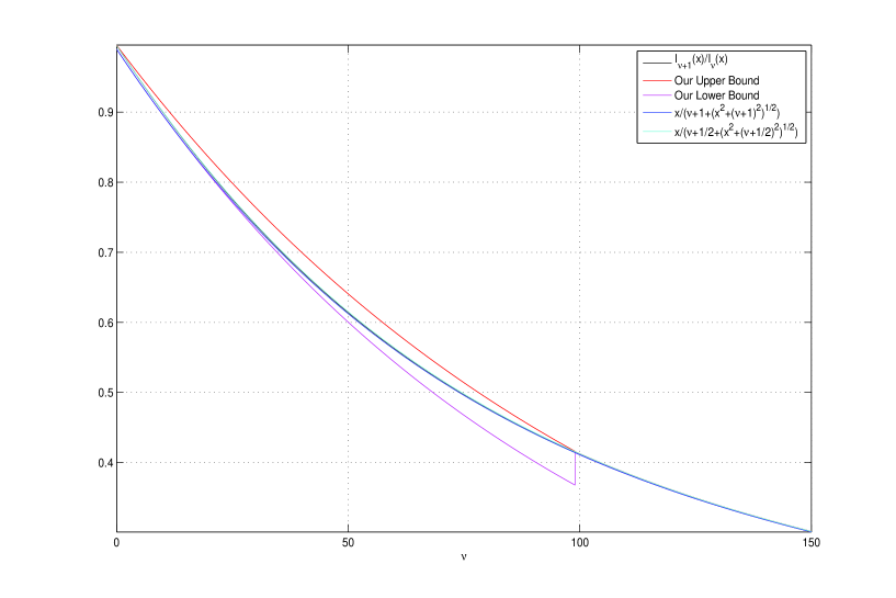
Figure 1: An illustration of the exponential-type bounds from Corollary 1 on ${I_{\nu+1}(x)}/{I_{\nu}(x)}$ for $x=100$, over the interval $[0,150]$ taken in steps of $0.015$. For $\nu+1\leq x$, we apply the bounds from Corollary 1, after which we use the lower and upper bounds ${x}/(\nu+1+\sqrt{x^{2}+(\nu+1)^{2}})$ and ${x}/(\nu+\frac{1}{2}+\sqrt{x^{2}+\left(\nu+\frac{1}{2}\right)^{2}})$, respectively. For comparison, we also plot these latter bounds for $\nu+1\leq x$, and note that due to how precise these bounds are for any $\nu$, the black, blue, and cyan curves nearly coincide.

2.2 Bounds on $H(\nu,x)$

The bounds in Section 2.1 on $I_{\nu+1}(x)/I_{\nu}(x)$ have extremely nice algebraic properties suitable for evaluation of products. This allows us to obtain explicit and interpretable bounds on $H(\nu,x)$.

Recall our program outlined in Section 1: for any $\nu,x\geq 0$,

$$H(\nu,x) =\begin{cases}\sum_{n=1}^{\infty}\prod_{k=0}^{n-1}\frac{I_{\nu+k+1}(x)}{I_{\nu+k}(x)}&[\nu]+2>[x]\\ \sum_{n=1}^{[x]-[\nu]-1}\prod_{k=0}^{n-1}\frac{I_{\nu+k+1}(x)}{I_{\nu+k}(x)}+\sum_{n=[x]-[\nu]}^{\infty}\prod_{k=0}^{[x]-[\nu]-2}\frac{I_{\nu+k+1}(x)}{I_{\nu+k}(x)}\prod_{k=[x]-[\nu]-1}^{n-1}\frac{I_{\nu+k+1}(x)}{I_{\nu+k}(x)}&[\nu]+2\leq[x]\enskip.\end{cases}$$

Using our bounds on $I_{\nu+1}(x)/I_{\nu}(x)$ in Corollary 1, the first term in the regime $[\nu]+2\leq[x]$ behaves like a sum of discrete Gaussians. The second term in the regime $[\nu]+2\leq[x]$ and the term in the regime $[\nu]+2>x$ are ”tail”-like quantities, and a simple geometric series-type argument using (10) suffices to capture the behavior of $H(\nu,x)$. In fact, such a geometric series-type argument holds for any $\nu\geq 0$, and we give the full result which will be useful for comparison.

Theorem 1

Let $\nu,x\geq 0$ and $H(\nu,x)$ be defined as in (1). Then, (4), (5), (6) and (7) hold.

Proof of Theorem 1:

1. We first prove (4). Note that

   $$H(\nu,x)=\frac{I_{\nu+1}(x)}{I_{\nu}(x)}(1+H(\nu+1,x))\enskip,$$

   which in view of (10) yields,

   $$F(\nu+1,x)(1+H(\nu+1,x))\leq H(\nu,x)\leq F\left(\nu+\frac{1}{2},x\right)(1+H(\nu+1,x))\enskip.$$ (11)

   Next, we have

   $$H(\nu+1,x) =\sum_{n=1}^{\infty}\prod_{k=1}^{n}\frac{I_{\nu+k+1}(x)}{I_{\nu+k}(x)}$$

   $$\leq\sum_{n=1}^{\infty}\prod_{k=1}^{n}\frac{x}{\nu+k+\frac{1}{2}+\sqrt{\left(\nu+k+\frac{1}{2}\right)^{2}+x^{2}}}$$

   $$\leq\sum_{n=1}^{\infty}\left(\frac{x}{\nu+\frac{3}{2}+\sqrt{\left(\nu+\frac{3}{2}\right)^{2}+x^{2}}}\right)^{n}$$

   $$=\sum_{n=1}^{\infty}F\left(\nu+\frac{3}{2},x\right)^{n}\enskip,$$

   so that

   $$1+H(\nu+1,x)\leq\sum_{n=0}^{\infty}F\left(\nu+\frac{3}{2},x\right)^{n}=\frac{1}{1-F\left(\nu+\frac{3}{2},x\right)}\enskip.$$

   Thus,

   $$H(\nu,x)\leq\frac{F\left(\nu+\frac{1}{2},x\right)}{1-F\left(\nu+\frac{3}{2},x\right)}$$

   yielding the upper bound in (4).

   For the lower bound, note that using (10),

   $$F(\nu+2,x)\leq\frac{I_{\nu+2}(x)}{I_{\nu+1}(x)}\leq H(\nu+1,x)\enskip,$$

   which in view of (11) implies

   $$F(\nu+1)(1+F(\nu+2,x))\leq H(\nu,x)\enskip.$$

   This completes the proof of (4).

2. Next, we prove (5), (6) and (7). Note that using an iterated product, we may write

   $$H(\nu,x)=\sum_{n=1}^{\infty}\frac{I_{\nu+n}(x)}{I_{\nu}(x)}=\sum_{n=1}^{\infty}\prod_{k=0}^{n-1}\frac{I_{\nu+k+1}(x)}{I_{\nu+k}(x)}$$

   so that for $[\nu]+2\leq[x]$,

   $$H(\nu,x) =\sum_{n=1}^{[x]-[\nu]-1}\prod_{k=0}^{n-1}\frac{I_{\nu+k+1}(x)}{I_{\nu+k}(x)}+\sum_{n=[x]-[\nu]}^{\infty}\prod_{k=0}^{[x]-[\nu]-2}\frac{I_{\nu+k+1}(x)}{I_{\nu+k}(x)}\prod_{k=[x]-[\nu]-1}^{n-1}\frac{I_{\nu+k+1}(x)}{I_{\nu+k}(x)}$$ (12)

   $$=\sum_{n=1}^{[x]-[\nu]-1}\prod_{k=0}^{n-1}\frac{I_{\nu+k+1}(x)}{I_{\nu+k}(x)}+\prod_{k=0}^{[x]-[\nu]-2}\frac{I_{\nu+k+1}(x)}{I_{\nu+k}(x)}\sum_{n=[x]-[\nu]}^{\infty}\prod_{k=[x]-[\nu]-1}^{n-1}\frac{I_{\nu+k+1}(x)}{I_{\nu+k}(x)}\enskip.$$

   First, we deal with the sum in the second term. Using similar arguments as above for the upper bound in the first part of the theorem, we can write

   $$\sum_{n=[x]-[\nu]}^{\infty}\prod_{k=[x]-[\nu]-1}^{n-1}\frac{I_{\nu+k+1}(x)}{I_{\nu+k}(x)}$$

   $$\leq\sum_{n=[x]-[\nu]}^{\infty}\prod_{k=[x]-[\nu]-1}^{n-1}\frac{x}{\nu+k+\frac{1}{2}+\sqrt{(\nu+k+\frac{1}{2})^{2}+x^{2}}}$$

   $$=F\left([x]+\nu_{f}-\frac{1}{2}\right)\cdot\left(1+\sum_{n=[x]-[\nu]}^{\infty}\prod_{k=[x]-[\nu]}^{n}\frac{x}{\nu+k+\frac{1}{2}+\sqrt{(\nu+k+\frac{1}{2})^{2}+x^{2}}}\right)$$

   $$\leq F\left([x]+\nu_{f}-\frac{1}{2}\right)\cdot\left(1+\sum_{n=[x]-[\nu]}^{\infty}\left(\frac{x}{[x]+\nu_{f}+\frac{1}{2}+\sqrt{([x]+\nu_{f}+\frac{1}{2})^{2}+x^{2}}}\right)^{n+1-([x]-[\nu])}\right)$$

   $$=\frac{F\left([x]+\nu_{f}-\frac{1}{2}\right)}{1-F\left([x]+\nu_{f}+\frac{1}{2},x\right)}\enskip.$$

   Similar arguments as in the lower bound for $[\nu]+2>[x]$ yield,

   $$\sum_{n=[x]-[\nu]}^{\infty}\prod_{k=[x]-[\nu]-1}^{n-1}\frac{I_{\nu+k+1}(x)}{I_{\nu+k}(x)}$$

   $$\geq\frac{I_{[x]+\nu_{f}}(x)}{I_{[x]+\nu_{f}-1}(x)}\left(1+\frac{I_{[x]+\nu_{f}+1}(x)}{I_{[x]+\nu_{f}}(x)}\right)$$

   $$\geq F([x]+\nu_{f},x)(1+F([x]+\nu_{f}+1,x))\enskip.$$

   Thus,

   $$H(\nu,x)\leq\sum_{n=1}^{[x]-[\nu]-1}\prod_{k=0}^{n-1}\frac{I_{\nu+k+1}(x)}{I_{\nu+k}(x)}+\prod_{k=0}^{[x]-[\nu]-2}\frac{I_{\nu+k+1}(x)}{I_{\nu+k}(x)}\frac{F\left([x]+\nu_{f}-\frac{1}{2}\right)}{1-F\left([x]+\nu_{f}+\frac{1}{2},x\right)}$$

   and

   $$H(\nu,x)\geq\sum_{n=1}^{[x]-[\nu]-1}\prod_{k=0}^{n-1}\frac{I_{\nu+k+1}(x)}{I_{\nu+k}(x)}+\prod_{k=0}^{[x]-[\nu]-2}\frac{I_{\nu+k+1}(x)}{I_{\nu+k}(x)}F([x]+\nu_{f},x)(1+F([x]+\nu_{f}+1,x))\enskip.$$

   Next, note that, each term in each of the products above have $\nu+k+1\leq x$, since the largest $k$ can be is $k=[x]-[\nu]-2$ and $\nu+([x]-[\nu]-2)+1=[x]+\nu_{f}-1\leq x$. Thus, we may apply Corollary 1 to obtain

   $$\prod_{k=0}^{[x]-[\nu]-2}\frac{I_{\nu+k+1}(x)}{I_{\nu+k}(x)} \leq\prod_{k=0}^{[x]-[\nu]-2}e^{-\alpha_{0}\frac{\nu+k+\frac{1}{2}}{x}}$$

   $$=\exp\left(-\frac{\alpha_{0}}{x}\left(\left(\nu+\frac{1}{2}\right)\left([x]-[\nu]-1\right)+\frac{\left([x]-[\nu]-1\right)\left([x]-[\nu]-2\right)}{2}\right)\right)$$

   $$=\exp\left(-\frac{\alpha_{0}}{2x}\left([x]-[\nu]-1\right)\left(2\nu+1+[x]-[\nu]-2\right)\right)$$

   $$=\exp\left(-\frac{\alpha_{0}}{2x}([x]-[\nu]-1)([x]+\nu+\nu_{f}-1)\right)\enskip.$$

   Likewise,

   $$\prod_{k=0}^{[x]-[\nu]-2}\frac{I_{\nu+k+1}(x)}{I_{\nu+k}(x)} \geq\prod_{k=0}^{[x]-[\nu]-2}e^{-\frac{\nu+k+1}{x}}=\exp\left(-\frac{([x]-[\nu]-1)([x]+\nu+\nu_{f})}{2x}\right)$$

   implying

   $$H(\nu,x)\leq\sum_{n=1}^{[x]-[\nu]-1}\prod_{k=0}^{n-1}\frac{I_{\nu+k+1}(x)}{I_{\nu+k}(x)}+e^{-\frac{\alpha_{0}}{2x}([x]-[\nu]-1)([x]+\nu+\nu_{f}-1)}\frac{F\left([x]+\nu_{f}-\frac{1}{2}\right)}{1-F\left([x]+\nu_{f}+\frac{1}{2},x\right)}$$

   and

   $$H(\nu,x)\geq\sum_{n=1}^{[x]-[\nu]-1}\prod_{k=0}^{n-1}\frac{I_{\nu+k+1}(x)}{I_{\nu+k}(x)}+e^{-\frac{([x]-[\nu]-1)([x]+\nu+\nu_{f})}{2x}}F([x]+\nu_{f},x)(1+F([x]+\nu_{f}+1,x))\enskip.$$

   Thus, it remains only to estimate the sum $\sum_{n=1}^{[x]-[\nu]-1}\prod_{k=0}^{n-1}{I_{\nu+k+1}(x)}/{I_{\nu+k}(x)}$. Using Corollary 1 again, we get

   $$\prod_{k=0}^{n-1}\frac{I_{\nu+k+1}(x)}{I_{\nu+k}(x)}\leq\prod_{k=0}^{n-1}e^{-\alpha_{0}\frac{\nu+k+\frac{1}{2}}{x}} =\exp\left(-\frac{\alpha_{0}}{2x}n(2\nu+n)\right)=\exp\left(-\frac{\alpha_{0}}{2x}[(n+\nu)^{2}-\nu^{2}]\right)\enskip.$$

   Applying the same technique used for the lower bound, we have

   $$e^{\frac{1}{2x}\left(\nu+\frac{1}{2}\right)^{2}}\sum_{n=1}^{[x]-[\nu]-1}e^{-\frac{1}{2x}\left(n+\nu+\frac{1}{2}\right)^{2}}\leq\sum_{n=1}^{[x]-[\nu]-1}\prod_{k=0}^{n-1}\frac{I_{\nu+k+1}(x)}{I_{\nu+k}(x)}\leq e^{\frac{\alpha_{0}\nu^{2}}{2x}}\sum_{n=1}^{[x]-[\nu]-1}e^{-\frac{\alpha_{0}}{2x}\left(n+\nu\right)^{2}}\enskip.$$ (13)

   Since both the upper and lower bounds are similar, we focus only on the upper bound. The lower bound can be treated similarly.

   $$\sum_{n=1}^{[x]-[\nu]-1}e^{-\frac{\alpha_{0}}{2x}\left(n+\nu\right)^{2}}$$

   $$=\sum_{k=[\nu]+1}^{[x]-1}e^{-\frac{\alpha_{0}}{2x}\left(k+\nu_{f}\right)^{2}}$$

   $$\leq\int_{[\nu]}^{[x]-1}e^{-\frac{\alpha_{0}}{2x}\left(y+\nu_{f}\right)^{2}}dy$$

   $$=\sqrt{\frac{2x}{\alpha_{0}}}\int_{\sqrt{\frac{\alpha_{0}}{2x}}\nu}^{\sqrt{\frac{\alpha_{0}}{2x}[x]-1+\nu_{f}}}e^{-u^{2}}du$$

   $$\leq\sqrt{\frac{2x}{\alpha_{0}}}\int_{\sqrt{\frac{\alpha_{0}}{2x}}\nu}^{\sqrt{\frac{\alpha_{0}}{2x}}x}e^{-u^{2}}du$$

   $$=\sqrt{\frac{2x}{\alpha_{0}}}\left[\int_{\sqrt{\frac{\alpha_{0}}{2x}}\nu}^{\infty}e^{-u^{2}}du-\int_{\sqrt{\frac{\alpha_{0}}{2x}}x}^{\infty}e^{-u^{2}}du\right]$$

   $$\leq\sqrt{\frac{2x}{\alpha_{0}}}\left[\frac{e^{-\frac{\alpha_{0}}{2x}\nu^{2}}}{\sqrt{\frac{\alpha_{0}}{2x}}\nu+\sqrt{\frac{\alpha_{0}}{2x}\nu^{2}+\frac{4}{\pi}}}-\frac{e^{-\frac{\alpha_{0}}{2x}x^{2}}}{\sqrt{\frac{\alpha_{0}}{2x}}x+\sqrt{\frac{\alpha_{0}}{2x}x^{2}+2}}\right]$$ (14)

   where after a $u$-substitution, we have used the inequality (see [1]),

   $$\frac{e^{-x^{2}}}{x+\sqrt{x^{2}+2}}\leq\int_{x}^{\infty}e^{-t^{2}}dt\leq\frac{e^{-x^{2}}}{x+\sqrt{x^{2}+\frac{4}{\pi}}}\;\;\;x\geq 0.$$

   From (13) and (14), we have

   $$H(\nu,x)\leq\sqrt{\frac{2x}{\alpha_{0}}}\left[\frac{1}{\sqrt{\frac{\alpha_{0}}{2x}}\nu+\sqrt{\frac{\alpha_{0}}{2x}\nu^{2}+\frac{4}{\pi}}}-\frac{e^{-\frac{\alpha_{0}}{2x}(x^{2}-\nu^{2})}}{\sqrt{\frac{\alpha_{0}}{2x}}x+\sqrt{\frac{\alpha_{0}}{2x}x^{2}+2}}\right]$$ (15)

   $$\hskip 72.26999pt+e^{-\frac{\alpha_{0}}{2x}([x]-[\nu]-1)([x]+\nu+\nu_{f}-1)}\frac{F\left([x]+\nu_{f}-\frac{1}{2}\right)}{1-F\left([x]+\nu_{f}+\frac{1}{2},x\right)}$$

   which can be written as

   $$H(\nu,x) \leq\frac{2x}{\alpha_{0}}\left[\frac{1}{\nu+\sqrt{\nu^{2}+\frac{8x}{\pi\alpha_{0}}}}-\frac{e^{-\frac{\alpha_{0}}{2x}(x^{2}-\nu^{2})}}{x+\sqrt{x^{2}+\frac{4x}{\alpha_{0}}}}\right]$$

   $$\hskip 72.26999pt+e^{-\frac{\alpha_{0}}{2x}([x]-[\nu]-1)([x]+\nu+\nu_{f}-1)}\frac{F\left([x]+\nu_{f}-\frac{1}{2}\right)}{1-F\left([x]+\nu_{f}+\frac{1}{2},x\right)}\enskip,$$

   yielding the upper bound in (7).

   To complete the proof then, we just need to prove the lower bound. Repeating similar arguments above,

   $$\sum_{n=1}^{[x]-[\nu]-1}e^{-\frac{1}{2x}\left(n+\nu+\frac{1}{2}\right)^{2}} \geq\int_{[\nu]+1}^{[x]-\nu+[\nu]+1}e^{-\frac{1}{2x}\left(y+\frac{1}{2}\right)^{2}}dy$$

   $$=\sqrt{2x}\int_{\frac{[\nu]+\frac{3}{2}}{\sqrt{2x}}}^{\frac{[x]-\nu+[\nu]+\frac{3}{2}}{\sqrt{2x}}}e^{-u^{2}}du$$

   $$\geq\sqrt{2x}\int_{\frac{\nu+\frac{3}{2}}{\sqrt{2x}}}^{\frac{x-\nu_{f}+\frac{3}{2}}{\sqrt{2x}}}e^{-u^{2}}du$$

   $$=\sqrt{2x}\left[\int_{\frac{1}{\sqrt{2x}}\left(\nu+\frac{3}{2}\right)}^{\infty}e^{-u^{2}}du-\int_{\frac{1}{\sqrt{2x}}\left([x]-\nu_{f}+\frac{3}{2}\right)}^{\infty}e^{-u^{2}}du\right]$$

   $$\geq\sqrt{2x}\left[\frac{e^{-\frac{1}{2x}\left(\nu+\frac{3}{2}\right)^{2}}}{\frac{1}{\sqrt{2x}}\left(\nu+\frac{3}{2}\right)+\sqrt{\frac{1}{2x}\left(\nu+\frac{3}{2}\right)^{2}+2}}\right.$$

   $$\left.\hskip 72.26999pt-\frac{e^{-\frac{1}{2x}\left([x]-\nu_{f}+\frac{3}{2}\right)^{2}}}{\frac{1}{\sqrt{2x}}\left([x]-\nu_{f}+\frac{3}{2}\right)+\sqrt{\frac{1}{2x}\left([x]-\nu_{f}+\frac{3}{2}\right)^{2}+\frac{4}{\pi}}}\right]\enskip.$$

Thus,

$$H(\nu,x)\geq e^{\frac{1}{2x}\left(\nu+\frac{1}{2}\right)^{2}}\sqrt{2x}\left[\frac{e^{-\frac{1}{2x}\left(\nu+\frac{3}{2}\right)^{2}}}{\frac{1}{\sqrt{2x}}\left(\nu+\frac{3}{2}\right)+\sqrt{\frac{1}{2x}\left(\nu+\frac{3}{2}\right)^{2}+2}}-\frac{e^{-\frac{1}{2x}\left([x]-\nu_{f}+\frac{3}{2}\right)^{2}}}{\frac{1}{\sqrt{2x}}\left([x]-\nu_{f}+\frac{3}{2}\right)+\sqrt{\frac{1}{2x}\left([x]-\nu_{f}+\frac{3}{2}\right)^{2}+\frac{4}{\pi}}}\right]$$

$$\hskip 216.81pt+e^{-\frac{([x]-[\nu]-1)([x]+\nu+\nu_{f})}{2x}}F([x]+\nu_{f},x)(1+F([x]+\nu_{f}+1,x))$$

$$\Rightarrow H(\nu,x)\geq e^{-\frac{1}{x}\left(\nu+1\right)}\frac{\sqrt{2x}}{\frac{1}{\sqrt{2x}}\left(\nu+\frac{3}{2}\right)+\sqrt{\frac{1}{2x}\left(\nu+\frac{3}{2}\right)^{2}+2}}$$

$$\hskip 72.26999pt-e^{-\frac{1}{2x}([x]-\nu-\nu_{f}+1)([x]+\nu-\nu_{f}+2)}\frac{\sqrt{2x}}{\frac{1}{\sqrt{2x}}\left([x]+\frac{3}{2}\right)+\sqrt{\frac{1}{2x}\left([x]+\frac{3}{2}\right)^{2}+\frac{4}{\pi}}}$$

$$\hskip 72.26999pt+e^{-\frac{([x]-[\nu]-1)([x]+\nu+\nu_{f})}{2x}}F([x]+\nu_{f},x)(1+F([x]+\nu_{f}+1,x))$$

which is the same as

$$H(\nu,x) \geq\frac{2xe^{-\frac{1}{x}\left(\nu+1\right)}}{\nu+\frac{3}{2}+\sqrt{\left(\nu+\frac{3}{2}\right)^{2}+4x}}-\frac{2xe^{-\frac{1}{2x}([x]-\nu-\nu_{f}+1)([x]+\nu-\nu_{f}+2)}}{[x]+\frac{3}{2}+\sqrt{\left([x]+\frac{3}{2}\right)^{2}+\frac{8x}{\pi}}}$$

$$\hskip 144.54pt+e^{-\frac{([x]-[\nu]-1)([x]+\nu+\nu_{f})}{2x}}F([x]+\nu_{f},x)(1+F([x]+\nu_{f}+1,x))\enskip.$$

Theorem 1 is proved.

$\square$

We illustrate the bounds (5), (6) and (7) on $H(\nu,x)$ in Figure 2 for $x=50$ and $\nu\in[0,70]$ in steps of $0.01$ and also plot the true values of $H(\nu,x)$ computed using MATLAB. For comparison, we also plot the $F(\nu,x)$ Lower/Upper bounds (4). The value $\epsilon=0.01$ is chosen to truncate the infinite sum of Bessel functions occurring in the numerator of $H(\nu,x)$ so that the terms beyond a certain index are less than $\epsilon$. We notice that there are regimes in $\nu$ for which our lower and upper bounds are worse and better than those using the geometric series-type bounds, but that near $\nu=0$, our bounds are substantially better, and is a result of the first difference in (6) and (7) obtained by the use of the exponential approximations (9) on $I_{\nu+1}(x)/I_{\nu}(x)$.

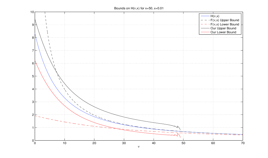
Figure 2: A comparison of our bounds (5), (6) and (7) on $H(\nu,x)$ compared to the true value of $H(\nu,x)$ for $x=50$ for $\nu\in[0,200]$ taken in steps of $0.01$. The $F(\nu,x)$ Lower/Upper bounds refer to those in (4). The value $\epsilon=0.01$ is chosen to truncate the infinite sum of Bessel functions occurring in the numerator of $H(\nu,x)$ so that the terms beyond a certain index are less than $\epsilon$. We note that near $\nu=0$, our bounds are substantially better than using (4) and scale like $\sqrt{x}$ for large $x$ which we would not have been able to obtain otherwise, and is the main purpose of this paper.

3 Main Results: Applications

In this section, we give some applications of Theorem 1. First, we briefly review the Skellam distribution, and relate it to the function $H(\nu,x)$.

Let $X_{1}\sim Pois(\lambda_{1})$ and $X_{2}\sim Pois(\lambda_{2})$ be two independent Poisson random variables with parameters $\lambda_{1}$ and $\lambda_{2}$, respectively. Then, the distribution of the random variable $W=X_{1}-X_{2}$ is called a Skellam distribution with parameters $\lambda_{1}$ and $\lambda_{2}$. We denote this by $W=X_{1}-X_{2}\sim Skellam(\lambda_{1},\lambda_{2})$ and have,

$$\mathbb{P}\left[W=n\right]=e^{-\left(\lambda_{1}+\lambda_{2}\right)}\left(\frac{\lambda_{1}}{\lambda_{2}}\right)^{\frac{n}{2}}I_{|n|}\left(2\sqrt{\lambda_{1}\lambda_{2}}\right).$$

The probabilistic value of $H(\nu,x)$ is now immediate: if $\lambda_{1}=\lambda_{2}=\lambda>0$, then $H(\nu,2\lambda)={\mathbb{P}\left[W>\nu\right]}/{\mathbb{P}\left[W=\nu\right]}$. The quantity

$$\mathcal{H}(\nu,2\lambda)=\frac{1}{H(\nu,2\lambda)+1}=\frac{\mathbb{P}\left[W=\nu\right]}{\mathbb{P}\left[W\geq\nu\right]}$$

is important in the actuarial sciences for describing the probability of death at time $\nu$ given death occurs no earlier than time $\nu$, and is known as the hazard function.

3.1 Application 1: Bounds on $\exp(-x)I_{\nu}(x)$ for $x\geq 0$ and $\nu\in\mathbb{N}$ and the Skellam$(\lambda_{1},\lambda_{2})$ Mass Function

Since the distribution of $W\sim Skellam(\lambda,\lambda)$ is symmetric, we have

$$\exp(-2\lambda)I_{0}(2\lambda)=\mathbb{P}\left[W=0\right]=\frac{1}{2H(0,2\lambda)+1}.$$ (16)

Thus, we may apply the bounds on ${I_{\nu+1}(x)}/{I_{\nu}(x)}$ and $H(\nu,x)$ given in Corollary 1 and Theorem 1, respectively, to obtain sharp upper and lower bounds on $\exp(-x)I_{0}(x)$ and hence on

$$\exp(-x)I_{\nu}(x)=\prod_{k=0}^{\nu-1}\frac{I_{k+1}(x)}{I_{k}(x)}\exp(-x)I_{0}(x)$$

for $\nu\in\mathbb{N}$. We note that this result therefore improves the asymptotic formula

$$\exp(-x)I_{\nu}(x)\sim\frac{1}{\sqrt{2\pi x}}\;\;\;{\rm as}\;\;\;x\rightarrow\infty$$

but only for $\nu\in\mathbb{N}$, and in particular, gives a bound on $\mathbb{P}\left[W=\nu\right]$ for $W\sim Skellam(\lambda,\lambda)$ by setting $x=2\lambda$.

Theorem 2

Set $\alpha_{0}=-\log(\sqrt{2}-1)\approx 0.8814.$ Then, for $\nu\in\mathbb{N}$ and $x\geq 0$,

1. If $\nu\leq x$,

   $$\frac{\exp((-\frac{\nu^{2}}{2x}\left(\frac{\nu+1}{\nu}\right))}{1+2\mathcal{U}(0,x)}\leq\exp(-x)I_{\nu}(x)\leq\frac{\exp(-\frac{\alpha_{0}}{2x}\nu^{2})}{1+2\mathcal{L}(0,x)}$$

2. If $\nu>x$,

   $$\frac{e^{-\frac{[x]^{2}}{2x}\left(\frac{[x]+1}{[x]}\right)}B\left([x]+\frac{x}{2}+1,\nu-[x]\right)\frac{(x/2)^{\nu-[x]}}{(\nu-[x]-1)!}}{1+2\mathcal{U}(0,x)}\leq e^{-x}I_{\nu}(x)\leq\frac{e^{-\frac{\alpha_{0}}{2x}[x]^{2}}B\left([x]+x+\frac{1}{2},\nu-[x]\right)\frac{x^{\nu-[x]}}{(\nu-[x]-1)!}}{{1+2\mathcal{L}(0,x)}}$$

   where $B(x,y)$ denotes the Beta function and $\mathcal{L}(\nu,x)$ and $\mathcal{U}(\nu,x)$ are the lower and upper bounds, respectively, from Theorem 1.

Proof of Theorem 2:

1. By Corollary 1, for $k+1\leq x$,

   $$e^{-\frac{k+1}{x}}\leq\frac{I_{k+1}(x)}{I_{k}(x)}\leq e^{-\alpha_{0}\frac{k+\frac{1}{2}}{x}}.$$

   so that for $\nu\leq x$,

   $$e^{-\frac{\nu^{2}}{2x}\left(\frac{\nu+1}{\nu}\right)}=\prod_{k=0}^{\nu-1}e^{-\frac{k+1}{x}}\leq\prod_{k=0}^{\nu-1}\frac{I_{k+1}(x)}{I_{k}(x)}\leq\prod_{k=0}^{\nu-1}e^{-\alpha_{0}\frac{k+\frac{1}{2}}{x}}=e^{-\frac{\alpha_{0}}{2x}\nu^{2}}\enskip.$$

   Thus,

   $$e^{-\frac{\nu^{2}}{2x}\left(\frac{\nu+1}{\nu}\right)}e^{-x}I_{0}(x)\leq e^{-x}I_{\nu}(x)\leq e^{-\alpha_{0}\frac{k+\frac{1}{2}}{x}}=e^{-\frac{\alpha_{0}}{2x}\nu^{2}}e^{-x}I_{0}(x)$$

   since

   $$e^{-x}I_{\nu}(x)=\prod_{k=0}^{\nu-1}\frac{I_{k+1}(x)}{I_{k}(x)}e^{-x}I_{0}(x).$$

   By (16) then, we have for $\nu\leq x$,

   $$\frac{e^{-\frac{\nu^{2}}{2x}\left(\frac{\nu+1}{\nu}\right)}}{1+2\mathcal{U}(0,x)}\leq e^{-x}I_{\nu}(x)\leq\frac{e^{-\frac{\alpha_{0}}{2x}\nu^{2}}}{1+2\mathcal{L}(0,x)}\enskip.$$

2. To prove the second assertion in theorem 2, notice that for $\nu>x$,

   $$\prod_{k=0}^{\nu-1}\frac{I_{k+1}(x)}{I_{k}(x)}=\prod_{k=0}^{[x]-1}\frac{I_{k+1}(x)}{I_{k}(x)}\prod_{k=[x]}^{\nu-1}\frac{I_{k+1}(x)}{I_{k}(x)}$$

   and each term in the first product has $k\leq x$ so that by the previous argument,

   $$e^{-\frac{[x]^{2}}{2x}\left(\frac{[x]+1}{[x]}\right)}\prod_{k=[x]}^{\nu-1}\frac{I_{k+1}(x)}{I_{k}(x)}\leq\prod_{k=0}^{\nu-1}\frac{I_{k+1}(x)}{I_{k}(x)}\leq e^{-\frac{\alpha_{0}}{2x}[x]^{2}}\prod_{k=[x]}^{\nu-1}\frac{I_{k+1}(x)}{I_{k}(x)}.$$

   Next,

   $$\frac{I_{k+1}(x)}{I_{k}(x)} \leq\frac{x}{k+\frac{1}{2}+\sqrt{\left(k+\frac{1}{2}\right)^{2}+x^{2}}}\leq\frac{x}{k+\frac{1}{2}+x}$$

   so that

   $$\prod_{k=[x]}^{\nu-1}\frac{I_{k+1}(x)}{I_{k}(x)}\leq\prod_{k=[x]}^{\nu-1}\frac{x}{k+\frac{1}{2}+x} =\frac{x^{\nu-[x]}\Gamma\left([x]+x+\frac{1}{2}\right)}{\Gamma\left(\nu+\frac{1}{2}+x\right)}$$

   $$=B\left([x]+x+\frac{1}{2},\nu-[x]\right)\frac{x^{\nu-[x]}}{(\nu-[x]-1)!}$$

   and similarly, using $\sqrt{a^{2}+b^{2}}\leq a+b$ for $a,b\geq 0$,

   $$\prod_{k=[x]}^{\nu-1}\frac{I_{k+1}(x)}{I_{k}(x)} \geq\prod_{k=[x]}^{\nu-1}\frac{x}{k+1+\sqrt{\left(k+1\right)^{2}+x^{2}}}$$

   $$\geq\prod_{k=[x]}^{\nu-1}\frac{x}{2(k+1)+x}$$

   $$=\prod_{k=[x]}^{\nu-1}\frac{x/2}{k+1+x/2}$$

   $$=\frac{(x/2)^{\nu-[x]}\Gamma\left([x]+1+\frac{x}{2}\right)}{\Gamma\left(\nu+\frac{x}{2}+1\right)}$$

   $$=B\left([x]+\frac{x}{2}+1,\nu-[x]\right)\frac{(x/2)^{\nu-[x]}}{(\nu-[x]-1)!}$$

   Thus, since $\exp(-x)I_{\nu}(x)=\prod_{k=0}^{\nu-1}{I_{k+1}(x)}/{I_{k}(x)}\exp(-x)I_{0}(x)$, we get

   $$\frac{e^{-\frac{[x]^{2}}{2x}\left(\frac{[x]+1}{[x]}\right)}B\left([x]+\frac{x}{2}+1,\nu-[x]\right)\frac{(x/2)^{\nu-[x]}}{(\nu-[x]-1)!}}{1+2\mathcal{U}(0,x)}\leq e^{-x}I_{\nu}(x)\leq\frac{e^{-\frac{\alpha_{0}}{2x}[x]^{2}}B\left([x]+x+\frac{1}{2},\nu-[x]\right)\frac{x^{\nu-[x]}}{(\nu-[x]-1)!}}{{1+2\mathcal{L}(0,x)}}.$$

   Thus theorem 2 is proved.

$\square$

A few remarks of Theorem 2 are in order:

1. One may simplify the upper bound using the bounds found in [3] on the Beta function, $B(x,y)$,

   $$\alpha\leq\frac{1}{xy}-B(x,y)\leq\beta$$

   where $\alpha=0$ and $\beta=0.08731\ldots$ are the best possible bounds.

2. By setting $x=2\sqrt{\lambda_{1}\lambda_{2}}$ and multiplying (1) and (2) in Theorem 2 through by

   $$\left(\sqrt{\frac{\lambda_{1}}{\lambda_{2}}}\right)^{\nu}\exp\left[-\left(\sqrt{\lambda_{1}}+\sqrt{\lambda_{2}}\right)^{2}\right],$$

   we obtain precise bounds on $\mathbb{P}\left[W=\nu\right]$ for $W\sim Skellam(\lambda_{1},\lambda_{2})$.

3. It’s important to note that if one were to use the geometric series-type bound (4) with $\nu=0$, that one would not achieve the behavior of $1/\sqrt{x}$ that we have in Theorem 2 which is indeed, guaranteed by the asymptotic $\exp(-x)I_{\nu}(x)\rightarrow 1/\sqrt{2\pi x}$ as $x\rightarrow\infty$ and exhibited by our non-asymptotic bounds on $H(\nu,x)$ in (6) and (7).

As an example of applying our bounds non-asymptotically, we plot $\exp(-x)I_{0}(x)$, its asymptotic ${1}/{\sqrt{2\pi x}}$ as $x\rightarrow\infty$, and the functions ${1}/({2\mathcal{L}(0,x)+1})$ and ${1}/(2\mathcal{U}(0,x)+1)$ in Figure 3. In steps of $1/100$, over the interval $[0,100]$, the top panel illustrates the behavior of all these functions over the interval $[0,100]$. We note that for large values of $x$, all functions values converge to zero, are extremely close, and are all on the order of $1/\sqrt{x}$ - something that one would not see by using instead the naive geometric-type bounds (4) with $\nu=0$. In the second panel, we restrict to the interval $[0,3]$ as our bounds transition across the line $[x]=2$. We note that for $[x]<2$, our upper bound is much more accurate than the asymptotic $1/\sqrt{2\pi x}$ and that in general is quite good.

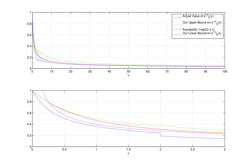
Figure 3: A comparison of our bounds on $\exp(-x)I_{0}(x)$ to the true value and the asymptotic $1/\sqrt{2\pi x}$. All plots are taken in steps of $1/100$ on a window of $[0,100]$. Top panel: behavior for $x\in[0,100]$. Bottom panel: the same plot, but over the interval $x\in[0,3]$. We note that for $[x]<2$, our upper bound is much more accurate than the asymptotic $1/\sqrt{2\pi x}$ and that in general is quite good. For large $x$, all curves $\sim 1/\sqrt{x}$ in agreement with the asymptotic $1/\sqrt{2\pi x}$, a behavior that would not have been achieved if instead one used the geometric series-type bounds (4) in place of $\mathcal{L}(0,x)$ and $\mathcal{U}(0,x)$.

3.2 Application 2: Concentration Inequality for the Skellam Distribution

We now present a concentration inequality for the $Skellam(\lambda,\lambda)$, the proof of which is a direct consequence of Theorem 2 and the identity,

$$\mathbb{P}\left[|W|>\nu\right]=1-\mathbb{P}\left[-\nu\leq W\leq\nu\right]=2H(\nu,2\lambda)\exp(-2\lambda)I_{\nu}(2\lambda).$$

Corollary 2

Let $W\sim Skellam(\lambda,\lambda)$, and define $\alpha_{0}=-\log\left(\sqrt{2}-1\right)$. Then,

1. If $\nu\leq x$,

   $$\frac{2\exp\left(-\frac{\nu^{2}}{4\lambda}\left(\frac{\nu+1}{\nu}\right)\right)}{1+2\mathcal{U}(0,2\lambda)}\leq\frac{\mathbb{P}\left[|W|>\nu\right]}{H(\nu,2\lambda)}\leq\frac{2\exp\left(-\frac{\alpha_{0}}{4\lambda}\nu^{2}\right)}{1+2\mathcal{L}(0,2\lambda)}$$

2. If $\nu>x$,

   $$\frac{2\exp\left(-\frac{[2\lambda]^{2}}{4\lambda}\left(\frac{[2\lambda]+1}{[2\lambda]}\right)\right)B\left([2\lambda]+\lambda+1,\nu-[2\lambda]\right)\frac{\lambda^{\nu-[2\lambda]}}{(\nu-[2\lambda]-1)!}}{1+2\mathcal{U}(0,2\lambda)} \leq\frac{\mathbb{P}\left[|W|>\nu\right]}{H(\nu,2\lambda)}$$

   $$\frac{2\exp\left(-\frac{\alpha_{0}}{4\lambda}[2\lambda]^{2}\right)B\left([2\lambda]+2\lambda+\frac{1}{2},\nu-[2\lambda]\right)\frac{(2\lambda)^{\nu-[2\lambda]}}{(\nu-[2\lambda]-1)!}}{{1+2\mathcal{L}(0,2\lambda)}} \geq\frac{\mathbb{P}\left[|W|>\nu\right]}{H(\nu,2\lambda)}$$

   where $B(x,y)$ denotes the Beta function and $\mathcal{L}(\nu,x)$ and $\mathcal{U}(\nu,x)$ are the lower and upper bounds, respectively, from Theorem 1.

4 Summary and Conclusions

In [25], the function $H(\nu,x)=\sum_{n=1}^{\infty}{I_{\nu+n}(x)}/{I_{\nu}(x)}$ for $x\geq 0$ and $\nu\in\mathbb{N}$ appears as a key quantity in approximating a sum of dependent random variables that appear in statistical estimation of network motifs as a Skellam$(\lambda,\lambda)$ distribution . A necessary scaling of $H(\nu,x)$ at $\nu=0$ of $\sqrt{x}$ is necessary, however, in order for the error bound of the approximating distribution to remain finite for large $x$. In this paper, we have presented a quantitative analysis of $H(\nu,x)$ for $x,\nu\geq 0$ necessary for these needs in the form of upper and lower bounds in Theorem 1. Our technique relies on bounding current estimates on ${I_{\nu+1}(x)}/{I_{\nu}(x)}$ from above and below by quantities with nicer algebraic properties, namely exponentials, while optimizing the rates when $\nu+1\leq x$ to maintain their precision.

In conjunction with the mass normalizing property of the $Skellam(\lambda,\lambda)$ distribution, we also give applications of this function in determining explicit error bounds, valid for any $x\geq 0$ and $\nu\in\mathbb{N}$, on the asymptotic approximation $\exp({-x})I_{\nu}(x)\sim{1}/{\sqrt{2\pi x}}$ as $x\rightarrow\infty$, and use them to provide precise upper and lower bounds on $\mathbb{P}\left[W=\nu\right]$ for $W\sim Skellam(\lambda_{1},\lambda_{2})$. In a similar manner, we derive a concentration inequality for the $Skellam(\lambda,\lambda)$ distribution, bounding $\mathbb{P}\left[|W|\geq\nu\right]$ where $W\sim Skellam(\lambda,\lambda)$ from above and below.

While we analyze the function $H(\nu,x)$ $\nu\in\mathbb{N}$, $x\geq 0$ for our purposes, we leave as future research the analysis for non integer $\nu$, as well as consideration of the generalized function

$$H(\nu,x)=\sum_{n=1}^{\infty}\left(\frac{\lambda_{1}}{\lambda_{2}}\right)^{\frac{n}{2}}\frac{I_{\nu+n}(2\sqrt{\lambda_{1}\lambda_{2}})}{I_{\nu}(2\sqrt{\lambda_{1}\lambda_{2}})}$$

that would appear for the $Skellam(\lambda_{1},\lambda_{2})$ distribution. We hope that the results laid here will form the foundation of such future research in this area.

It is also unknown as to whether normalization conditions for $\{\exp({-x})I_{\nu}(x)\}_{\nu=-\infty}^{\infty}$ induced by the $Skellam(\lambda,\lambda)$ hold for $\nu$ in a generalized lattice $\mathbb{N}+\alpha$, and if so, what the normalizing constant is. Such information would provide a key in providing error bounds on the asymptotic $\exp({-x})I_{\nu}(x)\sim{1}/{\sqrt{2\pi x}}$ for non-integer values of $\nu$.

References

- [1] M. Abramowitz and I.A. Stegun, Handbook of Mathematical Functions with Formulas, Graphs, and Mathematical Tables, Dover, New York, 1972.
- [2] D. E. Amos, Computation of Modified Bessel Functions and Their Ratios, Math. Comp. 28 (1974) 239-251.
- [3] H. Alzer. Sharp Inequalities for the Beta Function, Indagationes Mathematicae 12, 1 (2001) 15-21.
- [4] A.D. Barbour and L. Chen, An Introduction to Stein’s Method, Singapore University Press, Singapore, 2005.
- [5] A. Baricz, Bounds for Turanians of Modified Bessel Functions, arXiv:1202.4853 (2013).
- [6] A. Baricz, Bounds for Modified Bessel Functions of the First and Second Kinds, Proceedings of the Edinburgh Mathematical Society 52 (2010) 575-599.
- [7] A. Baricz and E. Neuman, Inequalities Involving Modified Bessel functions of the First Kind, Journal of Mathematical Analysis and Applications 332 (2007) 265-271.
- [8] A. Baricz and T. Pogany, On a Sum of Modifed Bessel Functions, arXiv:1301.5429 (2013).
- [9] A. Baricz and Y. Sun, New bounds for the Generalized Marcum Q-function, IEEE Transactions on Information Theory 55 (2009), 7.
- [10] M.C. Cranston and S.A. Molchanov, On a concentration inequality for sums of independent isotropic vectors, Electron. Commun. Probab. 17(27) (2012), 1-8.
- [11] S. B. Fotopoulos and K.J. Venkata, Bessel inequalities with applications to conditional log returns under GIG scale mixtures of normal vectors, Stat. Probab. Lett. 66 (2004) 117-125.
- [12] Y. Hwang, Difference-Based Image Noise Modeling Using Skellam Distribution, Pattern Analysis and Machine Intelligence 34, 7 (2012) 1329-1341.
- [13] N.L. Johnson, On an Extension of the Connection between Poisson and -distributions, Biometrika 46 (1959) 352-363.
- [14] M. Kanter, Probability inequalities for convex sets and multidimensional concentration, Journal of Multivariate Analysis 6, 2 (1976) 222-236.
- [15] D. Karlis and I. Ntzoufras, Analysis of sports data using bivariate Poisson models, Journal of the Royal Statistical Society Series D 52 (3) (2003) 381-393.
- [16] A. Laforgia and P. Natalini, Some Inequalities for Modified Bessel Functions, Journal of Inequalities and Applications (2010) 1-10.
- [17] Y. Luke, Inequalities for Generalized Hypergeometric Functions, Journal of Approximation Theory 5 (1972) 41-65.
- [18] E. Marchand and F. Perron, Improving on the MLE of a bounded normal mean, Ann. Statist. 29 (2001) 1078-1093.
- [19] E. Marchand and F. Perron, On the minimax estimator of a bounded normal mean, Stat. Probab. Lett. 58 (2002) 327-333.
- [20] E. Neuman, Inequalities Involving Modified Bessel Functions of the First Kind, Journal of Mathematical Analysis and Applications 171 (1992) 532-536.
- [21] C. Robert, Modified Bessel functions and their applications in probability and statistics, Stat. Probab. Lett. 9 (1990) 155-161.
- [22] J. Skellam, The frequency distribution of the difference between two Poisson variates belonging to different populations, Journal of the Royal Statistical Society Series A 109 (3) (1946) 296.
- [23] H. Simpson and S. Spector, Some monotonicity results for ratios of modified Bessel functions, Journal of Inequalities and Applications 42, 1 (1984) 95-98.
- [24] M. Simon and M.S. Alouini, Digital Communication Over Fadding Channels: A Unified Approach to Performance Analysis, Wiley, New York, 2000.
- [25] W. Viles, P. Balachandran and E. Kolaczyk. A Central Limit Theorem for Network Motifs. Manuscript.
- [26] P. Wolfe and K. Hirakawa, Efficient Multivariate Skellam Shrinkage for Denoising Photon-Limited Image Data: An Empirical Bayes Approach, Proc. IEEE Int. Conf. Image Processing (ICIP-09), Cairo, Egypt, Nov. 7-11 (2009) pp. 2961-2964.
- [27] L. Yuan and J.D. Kalbfleisch, On the Bessel distribution and related problems, Ann. Inst. Statist. Math. 52(3) (2000) 438-447.