Magnetic effects on spontaneous symmetry breaking/restoration in a toroidal topology

Abstract

We study temperature and finite-size effects on the spontaneous symmetry breaking/restoration for a scalar field model under the influence of an external magnetic field, at finite chemical potential. We use the 2PI formalism and consider the large-$N$ limit. We find that there is a minimal size of the system to sustain the broken phase, which diminishes as the applied field increases but is independent of the chemical potential. We analyze the critical curves and show that the magnetic field enhances the broken-phase regions, while increasing the chemical potential leads to a diminishement of the critical temperature.

I Introduction

Field theories defined on spaces with some of its dimensions compactified is interesting for several branches of theoretical physics. They can be related, for instance, to studies of finite-size scaling in phase transitions, to string theories or to phenomena involving extra dimensions in high and low energy physics cardy ; polchinski ; panilinha ; pani1 ; pani3 ; pani6 ; pani7 ; (g-2)NPB ; claudio . For a Euclidean $D$-dimensional space, compactification of some coordinates means that its topology is of the type $\Gamma_{D}^{d}=(S^{1})^{d}\times\mathbb{R}^{D-d}$, with $1\leq d\leq D$, $d$ being the number of compactified dimensions. Each of these compactified dimensions has the topology of a circle $S^{1}$. We refer to $\Gamma_{D}^{d}$ as a toroidal topology. Mathematical foundations to deal with quantum field theories on toroidal topologies are consolidated in recent developments AOP09 ; AOP11 . This provides a general framework for results from earlier works as for instance in Ademir ; AMS ; luc2 ; EPL12(1) ; PRD12 ; Emerson ; Isaque .

Here, in the framework of the two-particle irreducible (2PI) formalism CJT ; amelino in the Hartree–Fock approximation, we perform a study of magnetic effects for a field theory defined on a toroidal topology. The main interest of field theories defined on spaces with such a topology is that the simultaneous introduction of temperature and finite-size effects is allowed in a natural way, leading to size-dependent phase diagrams. We are particularly interested in how a magnetic background affects the size-dependent phase structure of the system; we present magnetic effects on spontaneous symmetry restoration induced by both temperature and spatial boundaries, at finite chemical potential. We will consider the system with a fixed squared mass parameter; within the toroidal formalism, the model is valid for the whole domain of temperatures, $0\leq T<\infty$.

II The 2PI formalism

We consider the model described by the Lagrangian density

$$\mathcal{L}=\frac{1}{2}\partial_{\mu}\varphi^{*}_{a}\partial^{\mu}\varphi_{a}+\frac{1}{2}m_{0}^{2}\varphi^{*}_{a}\varphi_{a}+\frac{u}{4!}\,(\varphi^{*}_{a}\varphi_{a})^{2}$$ (1)

in a Euclidean $D$-dimensional spacetime, where $m_{0}$ and $u$ are respectively the zero-temperature mass and the coupling constant in the absence of boundaries, of external magnetic field and at zero chemical potential. We consider the large-$N$ regime where $N\rightarrow\infty$ and $u\rightarrow 0$ but with $Nu$ finite and fixed. To simplify the notation, we drop out $a$-indices, summation over them being understood in field products. We proceed to approach symmetry restoration for this model following firstly the 2PI formalism CJT ; amelino in the absence of external field. In this case, the stationary condition for the effective action, in the Hartree–Fock approximation, leads to the gap equation

$$G^{-1}(\mathbf{x},\mathbf{x}^{\prime})=D^{-1}(\mathbf{x},\mathbf{x}^{\prime})+\frac{u}{2}\,G(\mathbf{x},\mathbf{x})\,\delta^{D}(\mathbf{x}-\mathbf{x}^{\prime}),$$ (2)

with $\mathbf{x},\mathbf{x}^{\prime}\in\mathbb{R}^{D}$. The Fourier-transformed propagators, $D({\bf k})$ and $G({\bf k})$, are given by

$$D({\bf k})=\frac{1}{{{\bf k}}^{2}+m_{0}^{2}+\frac{u}{2}\phi^{2}}\,;\;\;\;\;G({\bf k})=\frac{1}{{{\bf k}}^{2}+M^{2}}.$$ (3)

Here, $\phi=\left\langle 0\left|\sqrt{\varphi^{*}\varphi}\right|0\right\rangle$ is the vacuum expectation value of the quantum field $\varphi$ and $M$ is a momentum-independent effective mass.

In the 2PI formalism, the gap equation corresponds to the stationary condition and as such the effective mass depends on $\phi$ and conveys all daisy and superdaisy graphs contributing to $G({\bf k})$ CJT ; amelino . Nevertheless, in order to investigate symmetry restoration, we can take instead a particular constant value $M$ in the spontaneously broken phase. Renormalization of the mass and of the coupling constant can be performed with the procedure described in Ref. amelino . Then, defining the effective renormalized mass by ${\overline{m}}^{2}(\phi)=-m_{R}^{2}+(u_{R}/2)\phi^{2}$, where $m_{R}$ and $u_{R}$ are respectively the renormalized mass and the renormalized coupling constant, both at zero temperature and zero chemical potential, we can write the gap equation, in momentum space, in the large-$N$ limit as amelino ; Isaque

$${\overline{m}}^{2}(\phi)=M^{2}-\frac{\lambda_{R}}{2}\frac{1}{(2\pi)^{D}}\int d^{D}{k}\frac{1}{{{\bf k}}^{2}+M^{2}},$$ (4)

where

$$\lambda_{R}=\lim_{N\rightarrow\infty,u_{R}\rightarrow 0}(Nu_{R}).$$ (5)

In the following, we will generalize this equation to include effects of an external magnetic field as well as temperature, chemical potential and size effects. We shall consider the constant $\lambda_{R}$ as the physical renormalized coupling constant and focus only on the correction of the mass.

III Two-point function in the presence of a magnetic field

In the presence of an external magnetic field, the Lagrangian density in Eq. (1) becomes

$$\mathcal{L}=\frac{1}{2}{{D}}^{\dagger}_{\mu}\varphi^{*}{{D}}^{\mu}\varphi+\frac{1}{2}m_{0}^{2}\varphi^{*}\varphi+\frac{u}{4!}\,(\varphi^{*}\varphi)^{2},$$ (6)

where ${{D}}_{\mu}=\partial_{\mu}-ieA_{\mu}$ is the covariant derivative and $A_{\mu}$ is the potential of the external gauge field. We consider an uniform applied magnetic field $H$ and choose a gauge such that $A=(0,x_{1}H,0,0,\cdots)$. In this case, the part of the Hamiltonian quadratic in $\varphi$ becomes, after an integration by parts, $-\int d^{D}r\,\varphi^{\ast}\mathcal{D}\varphi$, where we have the differential operator lawrie1

$$\mathcal{D}=\nabla^{2}-2i\omega x_{1}\partial_{x_{2}}-\omega^{2}x_{1}^{2}-{m_{0}}^{2},$$ (7)

with $\omega=eH$ being the cyclotron frequency. Thus the natural basis to expand the field operators is the set of the normalized eigenfunctions of the operator $\mathcal{D}$, the Landau basis. Then, the free propagator can be written as lawrie1

$${\mathcal{G}}(\mathbf{x},\mathbf{x}^{\prime})=\int\frac{d^{D-2}{q}\,d\kappa}{(2\pi)^{D-1}}\,\sum_{\ell=0}^{\infty}\frac{\omega\,\xi_{\ell,\kappa,\mathbf{q}}(\mathbf{x})\,\xi_{\ell,\kappa,\mathbf{q}}^{\ast}(\mathbf{x}^{\prime})}{\mathbf{q}^{2}+(2\ell+1)\omega+m_{0}^{2}},$$ (8)

with the Landau eigenfunctions given by

$$\xi_{\ell,\kappa,\mathbf{q}}(\mathbf{x}) = \frac{1}{\sqrt{2^{\ell}{\ell}!}}\left(\frac{\omega}{\pi}\right)^{\frac{1}{4}}e^{i\mathbf{q}\cdot\mathbf{z}}\,e^{i\omega\kappa x_{2}}$$ (9)

$$\times\,e^{-\frac{1}{2}\omega(x_{1}-\kappa^{2})}\,H_{\ell}\left(\sqrt{\omega}(x_{1}-\kappa)\right),$$

where $H_{\ell}$ denote the Hermite polynomials, with cartesian coordinates, $\mathbf{x}=(x_{1},x_{2},\mathbf{z})$ and $\mathbf{q}$ the $(D-2)$-dimensional momentum associated to the vector $\mathbf{z}$ in the gauge we choose.

Following Ref. lawrie1 , we can extract the non-translational-invariant phase of the propagator (8) and write

$${\mathcal{G}}(\mathbf{x},\mathbf{x}^{\prime})=e^{i\omega(x_{1}+x_{1}^{\prime})(x_{2}-x_{2}^{\prime})/2}\,\bar{\mathcal{G}}(\mathbf{x}-\mathbf{x}^{\prime}),$$ (10)

where

$$\bar{\mathcal{G}}(\mathbf{x}-\mathbf{x}^{\prime}) = \int\frac{d^{D-2}{q}\,d\kappa}{(2\pi)^{D-1}}\,\sum_{\ell=0}^{\infty}\frac{\omega\,e^{i\mathbf{q}\cdot(\mathbf{z}-\mathbf{z}^{\prime})}}{\mathbf{q}^{2}+(2\ell+1)\omega+m_{0}^{2}}$$ (11)

$$\times\,\frac{1}{2^{\ell}\ell!}\sqrt{\frac{\omega}{\pi}}\,e^{i\omega\kappa(x_{2}-x_{2}^{\prime})}\,e^{-\frac{1}{4}[(x_{1}-x_{1}^{\prime})^{2}+4\kappa]}$$

$$\times\,H_{\ell}\left[\sqrt{\omega}\left(\small{\frac{1}{2}}(x_{1}-x_{1}^{\prime})-\kappa\right)\right]$$

$$\times\,H_{\ell}\left[\sqrt{\omega}\left(-\small{\frac{1}{2}}(x_{1}-x_{1}^{\prime})-\kappa\right)\right]$$

$$= \int\frac{d^{D}k}{(2\pi)^{D}}\,e^{i\mathbf{k}\cdot(\mathbf{x}-\mathbf{x}^{\prime})}\,\widetilde{\mathcal{G}}(\mathbf{k},\omega)\,.$$

Taking the coincidence limit, $\mathbf{x}=\mathbf{x}^{\prime}$, and using the orthonormality relations for the Hermite polynomials, we find

$$\widetilde{\mathcal{G}}(\mathbf{k},\omega)=2\pi\delta(k_{1})\delta(k_{2})\sum_{\ell=0}^{\infty}\frac{\omega}{\mathbf{k}^{2}+(2\ell+1)\omega+m_{0}^{2}}.$$ (12)

As a consequence, to introduce temperature and finite-size effects in the gap equation we are restricted to perform compactifications in the remaining $D-2$ coordinates; thus, to consider both effects we have to consider a space-time with dimension $D\geq 4$.

IV Mass corrections in a toroidal space in the presence of an external field

To take into account finite-size and chemical-potential effects, we consider first the changes introduced by the external field, given in Eq. (12) . To this end, let us remember that the parameter $M$ is an effective mass taken as a constant. In such a case, the changes due to the external applied constant magnetic field are introduced via the minimal coupling, $\partial_{\mu}\rightarrow D_{\mu}=\partial_{\mu}-ieA_{\mu}$ and we adopt the approximation of neglecting the corrections arising from the vertices involving the classical field $\phi$. This means that the integral $\int d^{D}{k}\,({\bf k}^{2}+M^{2})^{-1}$ in Eq. (4) should incorporate the magnetic field as dictated by Eq. (12), in such a way that Eq. (4) takes the form

$$\overline{m}^{2}(\phi;\omega)=M^{2}-\frac{\omega\lambda_{R}}{2}\sum_{\ell=0}^{\infty}\int\frac{d^{D-2}{q}}{(2\pi)^{D-2}}\frac{1}{{\bf q}^{2}+M_{\ell}^{2}(\omega)},$$ (13)

where $\overline{m}^{2}(\phi;\omega)$ is the $\omega$-dependent effective renormalized mass and $M_{\ell}^{2}(\omega)=M^{2}+(2\ell+1)\omega$.

In the sequel we will obtain the generalization of Eq. (13) in such a way as to include the toroidal topology as well as the chemical potential. Restoration of the symmetry will occur at the set of points in the toroidal space where $\overline{m}^{2}=0$.

We now proceed to generalize Eq. (13) to a theory defined on a space with a toroidal topology. In the $(D-2)$-dimensional system in thermal equilibrium at temperature $\beta^{-1}$ and with compactification of $d-1$ spatial coordinates (compactification lengths $L_{j}$, $j=2,3,\cdots d$). We have $\mathbf{z}=({\tau},z_{2},...,z_{d},\mathbf{w})$, where $\tau$ corresponds to imaginary time and $\mathbf{w}$ is a $(D-2-d)$-dimensional vector; the corresponding momentum is $\mathbf{q}=(q_{\tau},q_{2},...,q_{d},\mathbf{p})$, $\mathbf{p}$ being a $(D-2-d)$-dimensional vector in momentum space. We consider the simpler situation of $d=2$, the system at temperature $\beta^{-1}$ and one compactified spatial coordinate ($z_{2}\equiv z$) with a compactification length $L_{2}\equiv L$. Then the Feynman rules should be modified according to AOP09 ; AOP11

$$\int\frac{dq_{\tau}dq_{z}}{(2\pi)^{2}}f(q_{\tau},q_{z},\mathbf{p})\rightarrow\frac{1}{\beta L}\sum_{n_{\tau},n_{z}=-\infty}^{\infty}f_{\omega_{n_{\tau}},\omega_{n_{z}}}(\mathbf{p}),$$ (14)

where the function $f_{\omega_{n_{\tau}},\omega_{n_{z}}}(\mathbf{p})$ is obtained from $f(q_{\tau},q_{z},\mathbf{p})$ by the replacements $q_{\tau}\rightarrow 2n_{\tau}\pi/\beta-i\mu$ and $q_{z}\rightarrow 2n_{z}\pi/L$, where $\mu$ is the chemical potential. In this case, using Eq. (14), we can perform a suitable generalization of the procedure in amelino , to take into account finite-size, thermal and boundary effects in Eq. (13). The integral over the $(D-2)$-dimensional momentum in Eq. (13) becomes a double sum over $n_{\tau}$ and $n_{z}$ together with a ($D-4$)-dimensional integral over the remaining momentum $\mathbf{p}$.

Then, following steps similar to those in Ademir and using dimensional regularization to perform the integral, the renormalized $(T,L,\mu,\omega)$-dependent mass in the large-$N$ limit can be written in the form

$$\overline{m}^{2}(T,L,\mu,\omega)=M^{2}-\Sigma(T,L,\mu,\omega).$$ (15)

We introduce dimensionless parameters,

$$t=\frac{1}{M\beta},\,\chi=\frac{1}{ML},\,\gamma=\frac{\mu}{M},\,\delta=\frac{\omega}{M^{2}},\,\lambda=\frac{\lambda_{R}}{M^{4-D}}$$ (16)

and the notation $M_{\ell}^{2}(\omega)\equiv M_{\ell}^{2}(\delta)=M^{2}c_{\ell}^{2}(\delta)$, where

$$c_{\ell}(\delta)=\sqrt{1+(2\ell+1)\delta}.$$ (17)

Then in terms of the dimensionless quantities we have,

$$\frac{\Sigma(t,\chi,\gamma,\delta)}{M^{2}}=\lambda t\chi\delta\,\frac{\pi^{(D-4)/2}}{8\pi^{2}}\,\frac{\Gamma\left(s-\frac{D-4}{2}\right)}{\Gamma\left(s\right)}$$

$$\left.\times\sum_{\ell=0}^{\infty}Z_{2}^{h^{2}_{\ell}}\left(s-\frac{D-4}{2};t^{2},\chi^{2};b,0\right)\right|_{s=1},$$ (18)

where we define $b=i\gamma/2\pi t$ and $Z_{2}^{h^{2}}(\nu;\{a\},\{b\})=\sum_{n,l=-\infty}^{\infty}\left[a_{1}(n-b_{1})^{2}+a_{2}(l-b_{2})^{2}+h^{2}\right]^{-\nu}$ is an inhomogeneous Epstein–Hurwitz zeta function Elizalde , with $h^{2}_{\ell}=(2\pi)^{-1}c_{\ell}^{2}(\delta)$.

The Epstein–Hurwitz zeta functions have representations in the whole complex $s$-plane in terms of modified Bessel functions of the second kind $K_{\nu}$ Elizalde ; however, the first term of the Epstein–Hurwitz function in this representation implies that the first term in the correction to the mass is proportional to $\Gamma\left((4-D)/2\right)$, which is divergent for even dimensions $D\geq 4$ Ademir . This term is suppressed by a minimal subtraction, leading to a finite effective renormalized mass; notice that we call the quantities obtained after subtraction of this polar term renormalized quantities, in the sense of finite quantities, even if it is not a perturbative renormalization. For the sake of uniformity, this polar term is also subtracted for other dimensions, where no singularity exists, corresponding to a finite renormalization. Notice also that the polar term which is subtracted does not depend on $\beta$, $L$, $\mu$ and $\omega$.

This leads to the mass equation, written in terms of the above dimensionless parameters,

$$\frac{\overline{m}^{2}(t,\chi,\omega,\delta)}{M^{2}}=-1+{\lambda\frac{1}{\pi(2\pi)^{\frac{D-2}{2}}}}$$

$$\times\sum_{\ell=0}^{\infty}\left[\sum_{n=1}^{\infty}\cosh\left(\frac{\gamma n}{t}\right)\left(\frac{t}{nc_{\ell}(\delta)}\right)^{\frac{D-4}{2}}K_{\frac{D-4}{2}}\left(\frac{n}{t}c_{\ell}(\delta)\right)\right.$$

$$\left.+\sum_{n=1}^{\infty}\left(\frac{\chi}{nc_{\ell}(\delta)}\right)^{\frac{D-4}{2}}K_{\frac{D-4}{2}}\left(\frac{n}{\chi}c_{\ell}(\delta)\right)\right.$$

$$\left.+\,2\sum_{n,r=1}^{\infty}\cosh\left(\frac{\gamma n}{t}\right)\left(\frac{1}{c_{\ell}(\delta)\sqrt{\frac{n^{2}}{t^{2}}+\frac{r^{2}}{\chi^{2}}}}\right)^{\frac{D-4}{2}}\right.$$

$$\left.\times K_{\frac{D-4}{2}}\left(c_{\ell}(\delta)\sqrt{\frac{n^{2}}{t^{2}}+\frac{r^{2}}{\chi^{2}}}\right)\right].$$ (19)

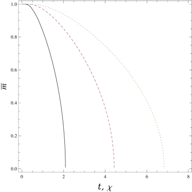
Figure 1: Plot of corrected mass $\overline{m}$ in Eq. (19) in units of $M$ as a function of $t$ ($\chi$), in the case of $\gamma=0.0$, for the values of the reduced magnetic field $\delta=0.01$, $\delta=0.5$ and $\delta=1.5$ (full, dashed and dotted lines, respectively). We fix $\lambda=1.0$, $\chi\,(t)=0.001$.

Figure 2: Reduced critical temperature versus reduced inverse size for a fixed value $\delta=1.0$ of the reduced applied field and (right to left curves) for reduced chemical potentials $\gamma=0.0,\,0.5,\,1.0$ (respectively full, dashed and dotted lines). We fix $\lambda=1.0$ The symmetry-breaking regions are below each curve.

Figure 3: Reduced critical temperature as a function of the reduced inverse size of the system, for a fixed value of the reduced chemical potential, $\gamma=0.5$ and the values of the reduced magnetic field $\delta=0.01$, $\delta=0.5$ and $\delta=1.5$ (respectively full, dashed and dot-dashed lines). We fix $\lambda=1.0$. The symmetry-breaking regions are below each curve.

Figure 4: Reduced critical temperature versus reduced chemical potential for a fixed value $\chi=0.5$ and for $\delta=0.01,\,0.5,\,1.5$ (respectively full, dashed and dotted lines). We fix $\lambda=1.0$ The symmetry-breaking regions are below each curve.

Figure 5: Reduced critical temperature versus the reduced chemical potential for three values of the reduced inverse size, $\chi=1.0$, $\chi=2.0$ and $\chi=2.5$, for a fixed value of the reduced applied field, $\delta=0.1$ (respectively full, dashed and dot-dashed lines). We fix $\lambda=1.0$ The symmetry-breaking regions are below each curve.

V Discussion

Now we analyze the effects of the finite-size and external magnetic field on the thermodynamic behavior of the system. In the general situation, the resulting equation does not allow an algebraic solution, and numerical evaluations are needed. For numerical evaluations, we fix the value $\lambda=1.0$ and take several values of the dimensionless parameters $t$, $\chi$, $\delta$, and $\gamma$.

In Fig. 1, it is illustrated the behavior of the effective corrected mass $\overline{m}$ defined in Eq. (19) for some values of the reduced magnetic field, as a function of the reduced temperature $t$ or the reduced inverse size $\chi$, at vanishing chemical potential. As it can be noted, the behavior of $\overline{m}$ with respect to the quantities $t$ and $\chi$ are similar for $\gamma=0$. The effective corrected mass decreases as $t$, $\chi$ increase in the same way. We see that for a given size, the critical temperature is higher for larger values of the applied field. Conversely, the minimal size sustaining the broken phase is smaller for higher values of the applied field.

To explore the results discussed above in more detail, we analyze the critical behavior of the system. Criticality is attained for $\overline{m}^{2}(t,\chi,\mu,\delta)=0$ in Eq. (19). The reduced critical temperature versus the reduced inverse size of the system $\chi$ is plotted in Fig 2. In this situation we have fixed the value of the reduced applied field at $\delta=1.0$, and the full, dashed and dotted lines represent the critical lines for different values of the reduced chemical potential: $\gamma=0.0,\,0.5,\,1.0$, respectively. We notice that the critical temperature diminishes as the size of the system increases, i.e. the broken phase is inhibited as the size of the system decreases. Besides, this figure strongly suggests that there is a minimal size of the system, $L_{0}$, (corresponding to a maximum allowed value of $\chi$, $\chi_{0}$), which is independent of the chemical potential, below which the symmetry breaking disappears. Also, the critical temperature depends on the density, in such a way that, for fixed values of the thickness and of the applied field, it is smaller for higher values of the chemical potential.

In Fig. 3, the reduced critical temperature versus the reduced inverse size of the system, $\chi$ is plotted for different values of the reduced applied field: $\delta=0.01$, $\delta=0.5$ and $\delta=1.5$, and for a fixed value of the reduced chemical potential, $\gamma=0.5$ (respectively full, dashed and dot-dashed lines). This figure shows that for higher applied fields the minimal thickness of the system for which the transition exists is smaller. In addition, we also see that the critical temperature is higher for a higher applied field. It means that the broken phase for a thinner system is favored as the magnetic field is increased; the magnetic field drives the system to the broken phase.

Another interesting result can be seen in Fig. 4, in which is plotted the reduced critical temperature versus the reduced chemical potential. The full, dashed and dot-dashed lines represent the critical lines for three values of the reduced applied field, $\delta=0.01$, $\delta=0.5$ and $\delta=1.5$, respectively, at fixed value of the reduced size, $\chi=0.5$. It suggests that the critical temperature decreases as the chemical potential increases and, as in Fig. 3, the broken phase is strengthened for stronger values of the applied field.

Finally, in Fig. 5 it is plotted again the reduced critical temperature versus the reduced chemical potential, but for three values of the reduced inverse size, $\chi=1.0$, $\chi=2.0$ and $\chi=2.5$, at the fixed value of the reduced applied field, $\delta=0.1$ (respectively full, dashed and dot-dashed lines). We see that the broken phase is inhibited for smaller sizes.

In summary, we have investigated how a magnetic background affects the size-dependent phase structure of the scalar field theory in the framework of 2PI formalism, in the Hartree–Fock approximation, considering the large-$N$ limit. We have found that the broken phase is strengthened for stronger values of the applied field. Also, the minimal size of the system, below which there is no phase transition, is smaller for greater values of the applied field. We thus conclude that the magnetic field drives the system to the broken phase.

References

- (1) J.L. Cardy (ed), Finite Size Scaling, North Holland, Amsterdam (1988).
- (2) J. Polchinski, Commun. Math. Phys. 104, 485 (2002).
- (3) G. Panico and M. Serone, J. High Energy Phys. 05, 024 (2005).
- (4) I. Antoniadis, Phys. Lett. B 246, 377 (1990).
- (5) G. Burdman and Y. Nomura, Nucl. Phys. B 656, 3 (2003).
- (6) N. Arkani-Hamed, A.G. Cohen, T. Gregoire, E. Katz, A.E. Nelson, and J.G. Walker, J. High Energy Phys. 08, 021 (2002); N. Arkani-Hamed, A.G. Cohen, E. Katz, and A.E. Nelson, J. High Energy Phys. 07, 034 (2002).
- (7) N. Arkani-Hamed, A.G. Cohen, and H. Georgi, Phys. Lett. B 513, 232 (2001).
- (8) A.J. Roy and M. Bander, Nucl. Phys. B 811, 353 (2009).
- (9) C. Ccapa Ttira, C.D. Fosco, A.P.C. Malbouisson, and I. Roditi, Phys. Rev. A 81, 032116 (2010).
- (10) F.C. Khanna, A.P.C. Malbouisson, J.M.C. Malbouisson, and A.E. Santana, Ann. Phys. (N.Y.) 324, 1931 (2009).
- (11) F.C. Khanna, A.P.C. Malbouisson, J.M.C. Malbouisson, and A.E. Santana, Ann. Phys. (N.Y.) 326, 2364 (2011).
- (12) A.P.C. Malbouisson, J.M.C. Malbouisson, A.E. Santana, Nucl. Phys. B 631, 83 (2002).
- (13) L.M. Abreu, M. Gomes, A J. da Silva, Phys. Lett.B 642, 551 (2006).
- (14) L.M. Abreu, A.P.C. Malbouisson, J.M.C. Malbouisson, A.E. Santana, Nucl. Phys. B 819, 127 (2009).
- (15) C.A. Linhares, A.P.C. Malbouisson, I. Roditi, EPL 98, 41001 (2012).
- (16) F.C. Khanna, A.P.C. Malbouisson, J.M.C. Malbouisson, A.E. Santana, Phys. Rev. D 85, 085015 (2012).
- (17) E.B.S. Corrêa, C.a. Linhares and A.P.C. Malbouisson, Phys. Lett. A 377, 1984 (2013).
- (18) C.A. Linhares, A.P.C. Malbouisson, J.M.C. Malbouisson and I. Roditi, Phys. Rev. D 86, 105022 (2012).
- (19) J.M. Cornwall, R. Jackiw, E. Tomboulis, Phys. Rev. D 10, 2428 (1974).
- (20) G. Amelino-Camelia, S.-Y. Pi, Phys. Rev. D 47, 2356 (1993).
- (21) I. D. Lawrie, Phys. Rev. Lett. 79, 131 (1997).
- (22) E. Elizalde, Ten Physical Applications of Spectral Zeta Functions, Springer, Berlin, (1995).