A topological method to characterize tapped granular media from the position of the particles.

Abstract

We use the first Betti number of a complex to characterize the morphological structure of granular samples in mechanical equilibrium. We analyze two-dimensional granular packings after a tapping process by means of both simulations and experiments. States with equal packing fraction obtained with different tapping intensities are distinguished after the introduction of a filtration parameter which determines the particles (nodes in the network) that are joined by an edge. We first use numerical simulations to characterize the effect of the precision in the particles localization by artificially adding different levels of noise in this magnitude. The outcomes obtained for the simulations are then compared with the experimental results allowing a clear distinction of experimental packings that have the same density. This is accomplished by just using the position of the particles and no other information about the possible contacts, or magnitude of forces.

Any dry granular material is a collection of macroscopic particles interacting between them mainly by contact forces. Due to this generality it is natural and appealing to consider a granular system as a graph where contacts between particles are edges, and the corresponding particles, nodes. Thus, defining such a network can be useful as it can be analyzed using the machinery of topology and modern complex networks theory newman . Based in the results of this analysis, the peculiarities and generalities of a granular ensemble can be characterized.

The contact network was used by Adler adler to study transport in porous media, and by Dodds dodds to analyze the porosity in random sphere packings. More recently, Basset et al. daniels use complex networks to understand sound propagation in granular materials. The network of contacts can also be used to characterize the evolution of granular media in dynamic situations. Walker, Tordesillas and collaborators have used simulations to deform granular samples under a variety of conditions and complex networks tools to study the resulting evolving networks walker1 ; walker2 ; tordesillas . In tordesillas1 the topological properties of the network were related to the process of strain localization, which leads to shear banding and material failure. Related with failure is the process of buckling of force chains studied in tordesillas2 , where it was revealed the importance of the presence of loops of contacts in the network. These contact loops were also proved to be crucial in the stability of tilted granular samples smart . Loops with an odd number of particles were, indeed, previously proved to be important for the rigidity of granular materials rivier .

Additionally to the contact network (the graph of all contacts), the force network can be also analyzed by the same methods. Indeed, the normalized contact force $f=F/<F>$ (where $F$ is the force present in a contact and $<F>$ the sample average) can be used to define as edge any contact bearing a force $f$ larger than some threshold value $f^{*}$ that can be tuned in the range $[0,f_{max}]$. Thus, for $f^{*}=0$ one recovers the contact network, while for larger values one obtains progressively diluted graphs. The analysis of the topology of the force networks has been shown very fruitful. Ostojic et al. ostojic used it to uncover a universality in the force distribution of granular packing. A variety of topological measures as function of $f^{*}$ were analyzed in arevalo3 in a static granular packing. The process of jamming in the light of the topology of force networks was studied in arevalo4 ; arevalo1 . Again, the role of loops in the network (particularly, third order loops) was proved to be relevant at the transition point, with third order loops behaving as an order parameter. Related to jamming is the question of isostaticity, which was analyzed using the force network by Walker et al. tordesillas3 .

Recently, Kondic and coworkers have analyzed the force network using topological invariants. In Kondic the zeroth Betti number $B0$, which measures the number of connected components (clusters), is used to study compressed granular samples. $B0$ is shown to be useful characterizing force networks obtained with varying density, friction and polydispersity of the grains. The zeroth Betti number is also used in kondic2 to analyze the role of interparticle friction in impact dynamics. Carlsson et al. carlsson used the zeroth and first Betti numbers to analyze a $2D$ system with small number of particles. Interestingly, they showed that critical points (where the topology can change) correspond to configurations in mechanical equilibrium.

It seems that studying contact and force networks offers a fruitful pathway for the understanding of static and dynamic properties of granular media. It is not completely clear, however, if these tools provide more (or better) information than other traditional measures. This question was addressed in Arevalotappingtriangulos where the topology of $2D$ granular samples in mechanical equilibrium was studied. It was already known pugnaloni1 that samples with the same density and number of particles may not be in the same state of equilibrium since the average force moment tensor can be different. In Arevalotappingtriangulos it was shown that the topology of the contact network (without information on the forces) was enough to distinguish these mechanically different states. Interestingly, traditional measurements based on particles’ positions –like the pair correlation function, the bond order parameter and the Voronoi tessellation– were shown to be less sensitive to capture such differences among different states with the same packing fraction.

In the same line is the recent work of Kramar et al. KramarGoulletKondicMichaikow who have used persistent homology to study the evolution of the force network in compressed granular materials. They track the evolution of the topology as a function of the density for different polydispersities and friction coefficients. Their approach is able to uncover the distinctive behavior displayed by different systems and, moreover, it is shown to be richer in information than the pair correlation function, the bond orientational order parameter and the distribution function of the forces.

Most of the works mentioned here are theoretical or consist on numerical simulations. In these conditions one has all the information necessary to construct the contact and force networks. However, under experimental conditions it is difficult to establish with certainty if there is contact between adjacent particles. It is then desirable to devise a method to study the contact network even in the case in which contacts cannot be exactly determined. In the present work we aim at precisely this goal using persistent homology.

Our system of study is a granular bed subject to tapping, which has been widely studied; experimentally nowak1 ; nowak2 ; richard ; schroter , by means of simulations ciamarra ; pugnaloni1 ; pugnaloni2 , and theoretically edwards1 . In pugnaloni1 ; pugnaloni2 it was shown that the packing fraction $\phi$ of the bed is not a monotonous function of the tapping intensity $\Gamma$. This rises the question of whether states with the same density are equivalent or not. A negative answer to this question was given in pugnaloni2 analyzing the force moment tensor of the system. As mentioned before, the same result can be obtained using the contact network. In the present work we use simulations and experiments to show that even when the contacts among the particles are not known, persistent homology allows to distinguish between states with the same density but in different mechanical equilibrium states.

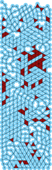
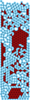
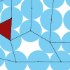
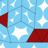
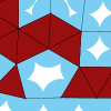
Figure 1: (Color online) At the top: three examples of the Vietoris-Rips complex (clique complex of the graph) obtained from the data given by the centers of particles of a sample obtained with $\Gamma=2$ which has an associated value of packing fraction $\phi=0.8$. Each column corresponds to a different value of the filtration parameter $\delta$. On the left $\delta=d$ the exact diameter of the particle, on the center $\delta=1.01d$ and on the right $\delta=1.05d$. On the bottom, a magnified region is shown evidencing the effect of increasing the filtration parameter in the Vietoris-Rips complex: some quadrilaterals in the middle picture are converted in triangles in the right picture. As explained in the text, the creation of a triangle implies an augment of $B1$ in the graph, and a decrease of $B1$ in the associated clique complex.

I Simulation and experimental methods

Simulation protocol: We use soft-particle molecular dynamics simulations in $2D$, in which static friction is implemented through the usual Cundall-Strack model cundall . The details of the implementation have been described elsewhere arevalo2 , and in the following we give the values of the interaction parameters used in the present work. In the normal direction of the contact we set the stiffness $k_{n}=10^{5}(mg/d)$ and damping parameter $\gamma_{n}=300(m\sqrt{g/d})$. In the tangential direction we set $k_{s}=\frac{2}{7}k_{n}$ for the stiffness and $\gamma_{s}=200(m\sqrt{g/d})$ for the damping parameter. The friction coefficient is fixed to $\mu=0.5$. We used reduced units with the diameter $d$ of the disks, the mass $m$ and the acceleration of gravity $g$. The integration time step is $\tau=10^{-4}\sqrt{d/g}$. The confining box has a width of $13.39d$ and infinitely high lateral walls. Simulations are run with $N=512$ monosized disks of diameter $d$.

The tapping is simulated by moving the confining box in the vertical direction following a sine shaped trajectory $A\sin(2\pi\nu t)[1-\Theta(2\pi\nu t-\pi)]$. We fix the frequency at the value $\nu=\pi/2(g/d)^{1/2}$ and control the tapping intensity $\Gamma=A(2\pi\nu)^{2}/g$ through the amplitude $A$. Once a tap is applied we decide that the system is in equilibrium implementing a criterium based on the stability of the contacts arevalo2 . At this point, particle positions are recorded which will be subsequently used to calculate both, the packing fraction and the network properties. In particular, the packing fraction is calculated in a slab of the bed that covers $50\%$ of the height of the column and is centered on the center of mass of the system. Then, a new tap is applied. Following this protocol we tap the bed $1000$ times for each reported value of the intensity. Averages are computed considering only the last $500$ taps of each run, where (in all the cases) the packing fraction has already became stationary, i.e. it has a well defined average.

In order to see how sensitive are our measurements to the lack of precision in the determination of the particle centers, we use a strategy consisting in adding controlled noise to the particles’ positions. From the original positions obtained from the simulations, we created sets of noisy data in the following manner. Given a value of $\alpha$ in $[0,0.1]$, we moved each center to a point at a random distance sampled from a uniform distribution in $[0,\alpha\,d]$ where $d$ is the diameter of the particles, and a random direction sampled from a uniform distribution in $[0,2\pi]$.

Experimental setup: A quasi 2D Plexiglass cell (width: 28 mm, height: 150 mm) was used to study the dependence of the packing on the intensity of shaking. The cell was filled with 600 alumina oxide spheres of diameter $d=1.00\;mm$. The side wall separation was 10% larger than the bead diameter in order to minimize the particle-wall friction and prevent arching in the transversal direction. The system was tapped with an electromagnetic shaker that provides a sine shaped pulse with a frequency ($\nu$) and an amplitude ($A$). The frequency was kept constant at ($\nu=30\;Hz$) and the amplitude was systematically modified in order to vary the tapping intensity $\Gamma=\frac{A(2\pi\nu)^{2}}{g}$. The latter was measured with a piezoelectric accelerometer attached to the base of the cell. High resolution digital images of the packings were taken after each tap. The center of each sphere was detected with an error smaller than $2\%$ of the particles diameter. The packing fraction of each packing was calculated by considering each grain as a disk of the corresponding effective diameter and then calculating the percentage of the area covered by the disks in a rectangular area 10% smaller than the size of the whole packing. In order to determine the average packing fraction, for each tapping amplitude we average over $200$ samples after reaching a stationary packing fraction. More details of the experimental protocol can be found in pugnaloni2 .

II Persistent Homology

Persistent homology is a tool that provides topological information of an object examined at different resolutions. We will give an ad-hoc description in the following paragraph and recommend the interested reader the sources Zomorodian ; EdelsbrunnerHarer ; Cannon for a more detailed and broad description. Since our data are 2D we will restrict all the relevant constructions to two dimensions.

Our data is the position of the centers of the particles in an experiment or simulation i.e. a set of points in the plane. The natural way to build a contact network is to consider the graph that has as vertices the mentioned set of points, and add an edge between a pair of vertices $p_{i}$, $p_{j}$, if the euclidean distance between them is less than the diameter $d$ of the particles $d(p_{i},p_{j})\leq d$. However this construction will miss some existing contacts and add some non existing contacts due to noise and/or numerical precision. To deal with this problem we construct a parametrized collection of graphs where the vertices are the same in all graphs (the above mentioned set of points), but edges in each graph are added whenever the distance between two points is less than a parameter $\delta\geq 0$.

Three particles that are in contact with each other form a “local perfect packing”. In order to keep track of these, we build a second structure associated with each one of the previously described graphs. If three nodes (particles) have all pairwise connections, i.e. edges between them form a triangle, we add a 2D-cell covering the triangle. We thus obtain a sort of “tesselation with holes” (see Fig. 1), called the clique complex of the graph in which the “holes” are the polygons formed by closed loops in the graph that are not triangles. This structure is a 2D-simplicial complex that is usually called the 2D-clique complex of the graph, and also the 2D-Vietoris-Rips complex of the dataset for the given filtration parameter.

Once we have a simplicial complex we can calculate its Betti numbers which are non negative integers, one for each dimension. Since our complexes live in the Euclidean plane, we are only interested in 0 dimensional and 1 dimensional Betti numbers. The 0-th Betti number ($B0$) of a complex is the number of connected components, and the 1-st Betti number ($B1$) counts the number of 1D-holes (the network polygons) in our complex. We will calculate the first Betti number (B1) of both the graph and the clique complex. In the graph, this accounts for the total number of 1D-holes, i.e. the number of polygons given by edges connecting data points in the graph. In the clique complex, B1 provides the number of uncovered polygons, i.e. polygons that are not triangles. Due to the presence of gravity, we expect to have a single connected component in most cases ($B0=1$), and thus we focus our study only in $B1$.

The effect of increasing the filtration parameter above the diameter of the particles in the $B1$ of the graph is that the development of new connections necessarily leads to the apparition of polygons and hence, to the increase of $B1$. In the clique complex, however, new connections may lead to the creation of polygons, but also to the covering of a triangle (and hence to a reduction of $B1$). We study filtration parameters in the range $d\leq\delta\leq 1.1d$ where $d$ denotes the diameter of the particles both, in the simulations and in the experiments. In this article, the homology calculations have been performed using the software javaplex javaplex , developed by the group of Applied and Computational Algebraic Topology of Stanford University.

III Simulation results

Let us start presenting in Fig. 2 already known results of the packing fraction $\phi$ dependence on the tapping intensity $\Gamma$ pugnaloni1 . There is a non monotonous dependence of $\phi$, which first decreases with $\Gamma$ and then, increases after a given value of the excitation parameter, $\Gamma_{min}$. This implies that states with the same packing fraction are obtained with very different tapping intensities. These states of equal $\phi$ have been demonstrated to display completely different stress properties pugnaloni2 , being also distinguishable by measuring the number of polygons of $3$, $4$, $5$, $6$… sides, obtained from the contact network Arevalotappingtriangulos .

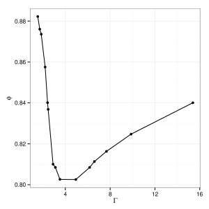
Figure 2: Mean packing fraction $\phi$ of the steady states as a function of the tap intensity $\Gamma$ obtained from numerical simulations.

In what follows we explain how persistent homology is useful to unveil topological differences among these states without the necessity of having an exact identification of all the contacts in the network. In Fig. 3 results of mean B1 (normalized by the number of particles) are presented versus $\Gamma$ for different values of the filtration parameter $\delta$ (as indicated in the legend) and different levels of noise (increasing from left to right panels). Looking at the results of the graph obtained for $\delta=1d$ without noise (circles in the top left panel), we realize the same qualitative behavior than the obtained for the total number of polygons in the contact network Arevalotappingtriangulos . At the same panel, we observe that increasing the value of $\delta$ leads to an augment of the values of B1 (the number of polygons increases) preserving the shape of the curves. Furthermore, when noise is added to the data the curve trends of $B1$ versus $\Gamma$ in the graph are maintained (top figures of Fig. 3). Importantly, the only effect that increasing the level of noise seems to have in the $B1$ graph is a downwards displacement of the curves (thus, the effect of random noise is to destroy polygons of all types). Adding $1\%$ noise strongly (slightly) affects $\delta=1.00d$ ($\delta=1.01d$) curves and has not apparent effect on curves obtained for higher values of $\delta$. Adding $3\%$ noise strongly affects $\delta=1.00d$, $\delta=1.01d$, and $\delta=1.02d$ curves; adding $5\%$ noise strongly affects curves with $\delta<1.05d$, and weakly affects $\delta=1.05d$. Despite the analysis of the noise effect may appear rather artificial at this point, it will be proved to be relevant when analyzing the experimental data which are, intrinsically, noisy.

A rather different behavior is obtained when displaying the values of B1 for the clique (bottom panels in Fig. 3). We will start explaining the case without noise (bottom left panel). Interestingly, although the trend displayed for $\delta=1d$ is similar to the obtained in the graph, a small increase of $\delta$ leads to a change of the curve trend: the minimum is transformed into a maximum. Considering that the only difference between the graph and the clique is that the latter does not account for triangles, the comparison of the correspondent curves provides interesting information. Focusing in the case of $\delta=1.01d$, the fact that the B1 of the clique increases with $\Gamma$ and then, after $\Gamma_{min}$ decreases again, implies that the number of polygons –without considering triangles- is maximum in $\Gamma_{min}$. At this same point, the total number of polygons (B1 of the graph) was proved to be minimum. This reflects that, the increase in B1 of the graph obtained when we move apart from $\Gamma_{min}$ is due to an augment in the number of triangles, and a consequent reduction in the number of the other polygons. A further increase of $\delta$ (which leads to increasing values of B1 in the graph) provokes a reduction of B1 in the clique without alteration of the curve trend. This evidences that most of the polygons that are build in the graph when increasing $\delta$ are, indeed, triangles.

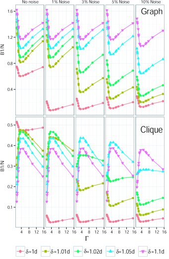
Figure 3: (Color online) Simulation results of the mean first Betti number (B1) normalized by the number of particles as a function of the tap intensity ($\Gamma$) for different values of the filtration parameter $\delta$ and different levels of noise in the data. At the top, results obtained from the graph and at the bottom, results obtained from the clique. The 95% confidence intervals for the mean of the normalized Betti numbers are of the size of the data points.

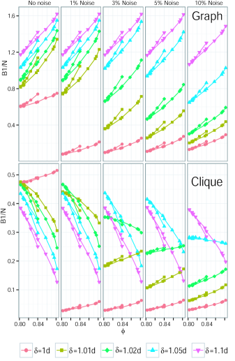
Figure 4: (Color online) Simulation results of the mean first Betti number (B1) normalized by the number of particles as a function of the packing fraction ($\phi$) for different values of the filtration parameter $\delta$ and different levels of noise in the data. At the top, results obtained from the graph and at the bottom, results obtained from the clique. The 95% confidence intervals for the mean of the normalized Betti numbers are of the size of the data points.

In the clique curves, the effect of adding noise is also notably different from that observed in the graph. If the value of $\delta$ is higher than the level of noise, the curves show a maximum and the values of B1 are reduced as $\delta$ increases. On the contrary, if $\delta$ is smaller than the noise level, the curves that originally displayed a maximum invert their shape and show a minimum – revealing a trend similar to the one observed for the case without noise and $\delta=1.00d$. This effect can be explained as follows. First, it should be recalled that for the case without noise, increasing $\delta$ leads to the development of a maximum in the clique curves as a consequence of the increase in the number of triangles. Considering this, it seems reasonable that adding a given amount of noise destroys some of the triangles creating polygons of any kind. The only way to compensate the addition of noise (and preserve the triangular structure in the network) is applying a sufficiently high filtration parameter.

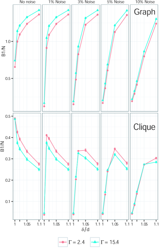
Figure 5: (Color online) Comparison of the mean first Betti number normalized by the number of particles for states with the same packing fraction obtained with different tap intensities ($\Gamma=2.4$ and $\Gamma=15.4$). Results obtained from simulations are presented versus the value of the filtration parameter for different levels of noise as indicated at the top of each figure. At the top, results obtained from the graph and at the bottom, results obtained from the clique. The error bars indicate the 95% confidence intervals for the mean of the normalized Betti numbers.

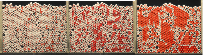
Figure 6: (Color online) Experimental photograph with the associated Vietoris-Rips complex for three different values of the filtration parameter. Left $\delta=d$, the estimated diameter of the particles, center $\delta=1.01d$ and right $\delta=1.05d$.

Since the objective of this manuscript is the implementation of persistent homology to distinguish among states with the same packing fraction, it seems more practical representing B1 (for different values of noise and filtration parameter) with respect to the packing fraction $\phi$ (Fig. 4). Interestingly, all the B1 data present two well defined branches; in this case the shorter one is for high $\Gamma$ and the longer one for low $\Gamma$ (see Fig. 2 to realize that the values of $\phi$ obtained above $\Gamma_{min}$ span over a smaller region than the ones obtained below $\Gamma_{min}$). These branches are more or less separated from each other depending on the values of noise and filtration parameter. Focusing first on the results of the graph without noise for $\delta=1.00d$, we observe that B1 increases with $\phi$, but this increment is more pronounced for the short branch (higher values of $\Gamma$). Comparing these results with the analogous of the clique, where the two branches are undistinguishable, we can conclude that the differences among the two branches are predominantly caused by the development of triangles (which are more abundant for high values of $\Gamma$). This result agrees whith the analysis carried out in Arevalotappingtriangulos .

The effect of increasing $\delta$ in the graph obtained without noise is just an augment of the values of B1 without changing the shape of the curves. Nevertheless, an exceedingly high filtration parameter like $\delta=1.10d$ seems to provoke a reduction in the separation between the two branches (down triangles in the top left graph of Fig. 4). The introduction of noise induces a decrease of the B1 values that mainly affects the curves obtained with a filtration parameter smaller than the level of noise. Notably, the decrease of B1 within a given curve is rather homogeneous, being independent on $\phi$. This effect was already appreciated in Fig. 3.

In the data obtained from the clique, the effect of adding noise and changing the filtration parameter may lead to an inversion of the tendency of the curves. Focusing first in the the case without noise, if $\delta>1.00d$ B1 decreases with $\phi$ in contrast to the case of $\delta=1.00d$. The origin of this change (which was already explained when describing the results displayed Fig 3) is based in the development of triangles for high values of $\phi$ attained for very high and very low values of $\Gamma$. The introduction of noise in the system leads to the transition from ascendent to descendent curves appearing for larger values of $\delta$. More interestingly, it seems that given a value of noise, the differences among the two branches in the clique networks are maximized for a filtration parameter higher or similar to the level of noise.

In order to check this idea, let us compare the outcomes of the B1 for two states that, being obtained with very different tap intensities, display the same packing fraction. This occurs, for example, for the states developed for $\Gamma=2.4$ and $\Gamma=15.4$ whose B1 values for different noise and filtration parameters are presented in Fig. 5. Clearly, the results obtained for the graph (top figures) reveal differences, being the values of B1 systematically higher for the highest tapping intensity. However, the differences become more or less important depending on the noise and the filtration parameter. For the data without additional noise, it seems that the outcomes of B1 are already different for $\delta=1d$. The differences are magnified for larger values of $\delta$ and seem to be minimized again for $\delta=1.1d$. Similar trends are observed when noise is added in the data. For these cases, however, it should be emphasized that the differences for $\delta=1d$ become almost nonexistent. Indeed, as the levels of noise augment, distinguishing among the states requires of larger values of $\delta$.

The results of the clique (bottom of Fig. 5) reveal that, opposite to the graph, the B1 values are systematically smaller for the case of the highest tap intensity. Again, this reveals that states with the same packing fraction develop more triangles when obtained at high tap intensities. Concerning the differences among the states when adding noise and changing the filtration parameter, the conclusions attained from the clique are similar to those already explained for the graph. In summary, for low levels of noise, differences are maximized for intermediate values of $\delta$. As the noise is increased, the values of $\delta$ from which differences appear also increase. The curve trends (monotonously decreasing for the case without added noise, and displaying a maximum when some noise is added) can be explained as a consequence of the development of triangles in the network. Indeed, the fact that for the case without noise, the B1 of the clique decreases with $\delta$ while B1 of the graph increases, is just a result of the development of triangles attained when increasing $\delta$. When adding noise, a drastic reduction is obtained in the B1 values of the clique for $\delta=1d$. This reduction was already observed in the graph, and thus it is due to the destruction of most of the polygons in the network. Of course, the values of $\delta$ which suffer modifications in the B1 outcomes, are only those smaller or similar to the level of noise. This leads to the non monotonicity of the curves.

From the numerical simulations we have learnt that the values of B1 obtained from both, the graph and the clique, for different levels of noise and filtration parameter, can be very useful to characterize the topology of the systems. Indeed, systems with the same packing fraction obtained with different intensities are clearly differentiated as they present different branches in the B1 versus $\phi$ plot. The important advance of the present work is that we can dodge the exact determination of all the contacts in the network. Remarkably, we have shown that, even in the presence of an important amount of noise in the particles’ positions, we can identify differences in the systems by appropriately defining a filtration parameter.

IV Experimental results

Once we have seen that states with the same packing fraction but obtained from very different tapping intensities can be distinguished even in the presence of considerable amount of noise, we turn on experimental data, which have a precision in the determination of the centers of the particles smaller than $2\%$ of their diameter. In Fig. 6 we show an experimental photograph with the Vietoris-Rips complex obtained using three values of the filtration parameter $\delta$. The one on the left uses $\delta=d$ leading to a quite unrealistic network due to the lack of precision in the determination of the particles’ centers. As $\delta$ increases, more contacts appear in the complex. Obviously, some of them are spurious as they are not real contacts, specially for the right picture where $\delta=1.05d$ is employed. These three pictures evidence the difficulty of properly defining a network of contacts from experimental data, suggesting the necessity of looking for alternatives that help to characterize the structure of the packing.

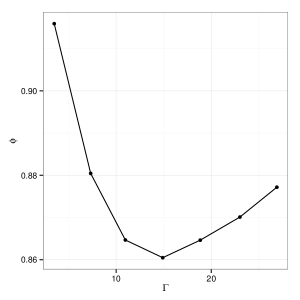
Figure 7: Experimental results of the mean packing fraction $\phi$ of the steady states as a function of the tap intensity $\Gamma$.

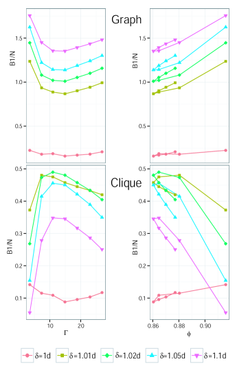
Figure 8: (Color online) Experimental results of the mean first Betti number (B1) normalized by the number of particles for different values of the filtration parameter $\delta$ as indicated in the legend. In the left column, B1 is presented versus the tap intensity $\Gamma$. In the right column B1 is presented versus the packing fraction of the sample $\phi$. At the top, results obtained from the graph and at the bottom, results obtained from the clique. In all cases, the 95% confidence intervals for the mean of the normalized Betti numbers are of the size of the data points.

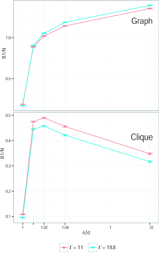
Figure 9: (Color online) Mean first Betti number versus $\delta$ for states with the same average packing fraction obtained with different tap intensities. As indicated in the legend, squares (triangles) are used for the state reached with $\Gamma=11$ ($\Gamma=18.8$). At the top, results obtained from the graph and at the bottom, results obtained from the clique. The error bars indicate the 95% confidence intervals for the mean of the normalized Betti numbers.

In Fig. 7 we show experimental results of the average packing fraction of the steady state as a function of $\Gamma$. As observed in the simulations, the packing fraction first decreases with $\Gamma$, and then increases after $\Gamma_{min}\approx 15$. Hence, states with the same $\phi$ are obtained with very different tapping intensities. The goal now is testing if these states can be distinguished by means of the average first Betti number as explained above. The evolution of B1 versus the tapping intensity is presented in the left column of Fig. 8 for both, the graph (top) and the clique (bottom). The outcomes strikingly resemble the numerical results obtained when adding $1\%$ noise to the particle’s position (second column in Fig. 3). As in the simulations, in the graph, the B1 curve obtained for $\delta=1.00d$ is significatively below the curves obtained for higher $\delta$. In addition, in the clique, the curve for $\delta=1.00d$ shows a minimum at $\Gamma_{min}$ that is converted into a maximum for $\delta=1.01d$. As explained in the previous section, this maximum is consequence of the presence of triangles in the network which is specially important for very high and low values of $\Gamma$ (those that produce large values of $\phi$).

The accordance of the experimental data with the numerical results displayed for the case of $1\%$ noise is confirmed by the plots of B1 versus $\phi$ (right column of Fig. 8). Surely, the graph shows an increase of B1 with $\phi$ independently on the value of $\delta$, but the two developed branches are clearly distinguished for values of the filtration parameter $\delta>1.00d$. In the clique, for $\delta>1.00d$, B1 decreases with $\phi$ as a consequence of the presence of triangles as explained previously. Again, increasing the value of $\delta$ we can achieve a clear differentiation among the two branches obtained in the B1 versus $\phi$ plot.

Finally, in Fig. 9 we compare the experimental values of B1 for two states with the same packing fraction but obtained at different tap intensities, i.e. $\Gamma=11$ and $\Gamma=18.8$ for the left and right sides of $\Gamma_{min}$. In the graph, the B1 values obtained for the highest $\Gamma$ are systematically above those obtained for the lowest $\Gamma$. This trend is reversed for the clique, where the B1 values obtained for the highest $\Gamma$ are systematically below those obtained for the lowest $\Gamma$. This behavior is in perfect agreement with numerical simulations, and can be attributed to the number of triangles developed in the network which is more important for the higher value of $\Gamma$. Interestingly, it is observed that a good election of the filtration parameter is crucial in order to differentiate among states with the same packing fraction. Once more, the experimental results are compatible with the outcomes of the simulations with a noise of approximately $1\%$. This implies that values of $\delta>1.01d$ are necessary to observe an enhancement of the differences among the two states.

V Conclusions

In this work, we have shown that the first Betti number of the graph and the clique (the Vietoris-Rips complex) can be satisfactorily used to characterize granular packings. Using a filtration parameter that defines whether or not two particles in the sample (nodes) are joined by a link, we are able to differentiate among states that display the same packing fraction but which are, indeed, different. This is accomplished even when the contacts among the particles are not accesible due to the lack of precision in the determination of the particles’ positions. In the first part of the manuscript we have studied the B1 dependence on both $\Gamma$ and $\phi$ by means of numerical simulations where the particle’s position can be obtained with $10^{-8}d$ precision. Then, we have artificially introduced noise in the positions of the particles and characterized its effect in the observed behavior. Based on these results we have implemented the same techniques on experimental data, finding qualitative agreement with the numerical outcomes for the case of $1\%$ noise.

More importantly, the results reported in this work prove that an accurate determination of the contacts among the particles is not necessary to observe topological differences among states with the same packing fraction, but obtained with different tapping intensities. This result supposes an important step forward with respect to a previous one Arevalotappingtriangulos where the topological tool introduced to identify such differences is only available if the contact network is well defined. On the contrary, the topological approach introduced in this manuscript can be used to characterize experimental packing ensembles even where the contact network is not fully accessible due to the limited resolution of the experimental techniques.

- (1) M. E. J. Newman, SIAM Review 45, 167 (2003).
- (2) P. M. Adler, Int. J. Multiphase Flow 11, 91 (1985).
- (3) J. A. Dodds, J. Colloid. Interphase Sci. 77, 317 (1980).
- (4) D. S. Bassett, E. T. Owens, K. E. Daniels, M. A. Porter, Phys. Rev. E 86, 041306 (2012).
- (5) D. M. Walker and A. Tordesillas, Phys. Rev. E 85 011304 (2012).
- (6) D. M. Walker, A. Tordesillas, Int. J. Solids Struct. 47, 624 (2010).
- (7) D. M. Walker, A. Tordesillas, I. Einav, M. Small, Phys. Rev. E 84, 021301 (2011).
- (8) A. Tordesillas, D. M. Walker, E. Andò, G. Viggiani, P. Roy. Soc. Lond. A Mat. 469, 2152 (2013).
- (9) A. Tordesillas, D. M. Walker, Q. Lin, Phys. Rev. E 81, 011302 (2010).
- (10) A.G. Smart, J. M. Ottino, Phys. Rev. E 77, 041307 (2008).
- (11) N. Rivier, J. Non-Cryst. Solids 352, 42 (2006).
- (12) S. Ostojic, E. Somfai, B. Nienhuis, Nature 439, 828 (2006).
- (13) R. Arévalo, I. Zuriguel and D. Maza, Int. J. Of Bif. & Chaos 19, 695 (2009).
- (14) R. Arévalo, I. Zuriguel, and D. Maza, Phys. Rev. E 81, 041302 (2010).
- (15) R. Arévalo, I. Zuriguel, S. Ardanza-Trevijano, and D. Maza, Int. J. Of Bif. & Chaos 20, 897 (2010).
- (16) D. M. Walker, A. Tordesillas, C. Thornton, R. P. Behringer, J. Zhang, J. Peters, Gran. Matt. 13, 233 (2011).
- (17) L. Kondic, A. Goullet, C. O’Hern, M. Kramar, K. Mischaikow, and R. Behringer, Europhys. Lett. 97, 54001 (2012).
- (18) L. Kondic, X. Fang, W. Losert, C. S. O’Hern, R. P. Behringer, Phys. Rev. E. 85, 011305 (2012).
- (19) G. Carlsson, J. Gorham, , M. Kahle, J. Mason, Phys. Rev. E. 85, 011303 (2012).
- (20) R. Arévalo, L.A. Pugnaloni, I. Zuriguel, and D. Maza, Phys. Rev. E 87, 022203 (2013).
- (21) L. A. Pugnaloni, I. Sánchez, P. A. Gago, J. Damas, I. Zuriguel, and D. Maza, Phys. Rev. E 82 050301R (2010).
- (22) M. Kramar, A. Goullet, L. Kondic, and K. Mischaikow Phys. Rev. E. 87, 042207 (2013).
- (23) E. R. Nowak, J. B. Knight, E. Ben-Naim, H. M. Jaeger, and S. R. Nagel, Phys. Rev. E 57, 1971 (1998).
- (24) E. R. Nowak, J. B. Knight, M. L. Povinelli, H. M. Jaeger, and S. R. Nagel, Powder Technol. 94, 79 (1997).
- (25) Ph. Ribière, P. Richard, P. Philippe, D. Bideau, and R. Delannay, Eur. Phys. J. E 22, 249 (2007).
- (26) M. Schröter, D. I. Goldman, and H. L. Swinney, Phys. Rev. E 71, 030301 R (2005).
- (27) M. Pica Ciamarra, A. Coniglio, and M. Nicodemi, Phys. Rev. Lett. 97, 158001 (2006).
- (28) L. A. Pugnaloni, J. Damas, I. Zuriguel, and D. Maza, Papers in Physics 3, 030004 (2011).
- (29) S. F. Edwards and R. B. S. Oakeshott, Physica A 157, 1080 (1989).
- (30) P. A. Cundall, O. D. L. Strack, Geotechnique 29, 47 (1979).
- (31) R. Arévalo, D. Maza, and L. A. Pugnaloni, Phys. Rev. E 74, 021303 (2006).
- (32) G. Carlsson, Bull. Am. Math. Soc. 46, 255 (2012).
- (33) H. Edelsbrunner and J.L. Harer, Computational Topology (AMS, Providence, RI, 2010).
- (34) A.J. Zomorodian, Topology for computing, (Cambridge University Press, UK, 2005).
- (35) A. Tausz, M. Vejdemo-Johansson, and H. Adams, JavaPlex: A research software package for persistent (co)homology (2011) http://code.google.com/javaplex