Multiuser SM-MIMO versus Massive MIMO: Uplink Performance Comparison

Abstract

In this paper, we propose algorithms for signal detection in large-scale multiuser spatial modulation multiple-input multiple-output (SM-MIMO) systems. In large-scale SM-MIMO, each user is equipped with multiple transmit antennas (e.g., 2 or 4 antennas) but only one transmit RF chain, and the base station (BS) is equipped with tens to hundreds of (e.g., 128) receive antennas. In SM-MIMO, in a given channel use, each user activates any one of its multiple transmit antennas and the index of the activated antenna conveys information bits in addition to the information bits conveyed through conventional modulation symbols (e.g., QAM). We propose two different algorithms for detection of large-scale SM-MIMO signals at the BS; one is based on message passing and the other is based on local search. The proposed algorithms are shown to achieve very good performance and scale well. Also, for the same spectral efficiency, multiuser SM-MIMO outperforms conventional multiuser MIMO (recently being referred to as massive MIMO) by several dBs; for e.g., with 16 users, 128 antennas at the BS and 4 bpcu per user, SM-MIMO with 4 transmit antennas per user and 4-QAM outperforms massive MIMO with 1 transmit antenna per user and 16-QAM by about 4 to 5 dB at $10^{-3}$ uncoded BER. The SNR advantage of SM-MIMO over massive MIMO can be attributed to the following reasons: $(i)$ because of the spatial index bits, SM-MIMO can use a lower-order QAM alphabet compared to that in massive MIMO to achieve the same spectral efficiency, and $(ii)$ for the same spectral efficiency and QAM size, massive MIMO will need more spatial streams per user which leads to increased spatial interference.

Keywords – Large-scale MIMO systems, spatial modulation, SM-MIMO, massive MIMO, message passing, local search.

(a) SM-MIMO system.

(b) Massive MIMO system.

Figure 1: Large-scale multiuser SM-MIMO and massive MIMO system architectures.

I Introduction

Large-scale MIMO systems with tens to hundreds of antennas are getting increased research attention [1]-[4]. The following two characteristics are typical in conventional MIMO systems: $(i)$ there will be one transmit RF chain for each transmit antenna (i.e., on the modulation symbols (e.g., QAM). Spatial modulation MIMO (SM-MIMO) systems [5] differ from conventional MIMO systems in the following two aspects: $(i)$ in SM-MIMO there will be multiple transmit antennas but only one transmit RF chain, and $(ii)$ the index of the active transmit antenna will also convey information bits in addition to information bits conveyed through modulation symbols like QAM. The advantages of SM-MIMO include reduced RF hardware complexity, size, and cost.

Conventional multiuser MIMO systems with a large number (tens to hundreds) of antennas at the base station (BS) are referred to as ‘massive MIMO’ systems in the recent literature [4]. The users in a massive MIMO system can have one or more transmit antennas with equal number of transmit RF chains. In large-scale multiuser SM-MIMO systems also, the number of BS antennas will be large. The users in SM-MIMO will have multiple transmit antennas but only on RF chain. Figures 1(a) and 1(b) illustrate the large-scale multiuser SM-MIMO system (with $K$ users, $N$ BS antennas, $n_{t}$ transmit antennas per user, and $n_{rf}=1$ transmit RF chain per user) and massive MIMO system (with $K$ users, $N$ BS antennas, $n_{t}=1$ transmit antenna per user, and $n_{rf}=1$ transmit RF chains per user), respectively.

Several works have focused on single user point-to-point SM-MIMO systems ([6] and the references therein). Some works on multiuser SM-MIMO have also been reported [7]-[9]. An interesting result reported in [7] is that multiuser SM-MIMO outperforms conventional multiuser MIMO by several dBs for the same spectral efficiency. This work is limited to 3 users (with 4 antennas each) and 4 antennas at BS receiver. Also, only maximum likelihood (ML) detection is considered. This superiority of SM-MIMO over conventional MIMO attracts further investigations on multiuser SM-MIMO. In particular, investigations in the following two directions are of interest: $(i)$ large-scale SM-MIMO (with large number of users and BS antennas), and $(ii)$ detection algorithms that can scale and perform well in such large-scale SM-MIMO systems. In this paper, we make contributions in these two directions.

We investigate multiuser SM-MIMO with similar number of users and BS antennas envisaged in massive MIMO, e.g., tens of users and hundreds of BS antennas. Our contributions can be summarized as follows.

• Proposal of two different algorithms for detection of large-scale SM-MIMO signals at the BS. One algorithm is based on message passing referred to as MPD-SM (message passing detection for spatial modulation) algorithm, and the other is based on local search referred to as LSD-SM (local search detection for spatial modulation) algorithm. Simulation results show that these proposed algorithms achieve very good performance and scale well.

• Uplink performance comparison between SM-MIMO and massive MIMO for the same spectral efficiency. Simulation results show that SM-MIMO outperforms massive MIMO by several dBs; e.g., SM-MIMO has a 4 to 5 dB SNR advantage over massive MIMO at $10^{-3}$ BER for 16 users, 128 BS antennas, and 4 bpcu per user.

  The SNR advantage of SM-MIMO over massive MIMO is attributed to the following reasons: $(i)$ because of the spatial index bits, SM-MIMO can use a lower-order QAM alphabet compared to that in massive MIMO to achieve the same spectral efficiency, and $(ii)$ for the same spectral efficiency and QAM size, massive MIMO will need more spatial streams per user which leads to increased spatial interference.

The rest of the paper is organized as follows. The system model for multiuser SM-MIMO is presented in Section II. The proposed MPD-SM algorithm for detection of SM-MIMO signals and its performance are presented in Section III. In Section IV, the proposed LSD-SM algorithm and its performance are presented. Performance comparison between SM-MIMO and massive MIMO is presented in Sections III and IV. Conclusions are presented in Section V.

II Multiuser SM-MIMO system model

Consider a multiuser system with $K$ uplink users communicating with a BS having $N$ receive antennas, where $N$ is in the order of tens to hundreds. The ratio $\alpha=K/N$ is the system loading factor. Each user employs spatial modulation (SM) for transmission, where each user has $n_{t}$ transmit antennas but only one transmit RF chain (see Fig. 1(a)). In a given channel use, each user selects any one of its $n_{t}$ transmit antennas, and transmits a symbol from a modulation alphabet ${\mathbb{A}}$ on the selected antenna. The number of bits conveyed per channel use per user through the modulation symbols is $\lfloor\log_{2}|{\mathbb{A}}|\rfloor$. In addition, $\lfloor\log_{2}n_{t}\rfloor$ bits per channel use (bpcu) per user is conveyed through the index of the chosen transmit antenna. Therefore, the overall system throughput is $K(\lfloor\log_{2}|{\mathbb{A}}|\rfloor+\lfloor\log_{2}n_{t}\rfloor)$ bpcu. For e.g., in a system with $K=3$, $n_{t}=4$, 4-QAM, the system throughput is 12 bpcu.

The SM signal set ${\mathbb{S}}_{n_{t},{\mathbb{A}}}$ for each user is given by

$${\mathbb{S}}_{n_{t},{\mathbb{A}}}=\big{\{}{\bf s}_{j,l}:j=1,\cdots,n_{t},\ \ l=1,\cdots,|{\mathbb{A}}|\big{\}},$$

$$\mbox{s.t.}\ \ {\bf s}_{j,l}=[0,\cdots,0,\underbrace{s_{l}}_{{\scriptsize{\mbox{$j$th coordinate}}}},0,\cdots,0]^{T},\ \ s_{l}\in\mathbb{A}.$$ (1)

For e.g., for $n_{t}=2$ and 4-QAM, ${\mathbb{S}}_{n_{t},{\mathbb{A}}}$ is given by

$${\mathbb{S}}_{2,\mbox{{\tiny 4-QAM}}} = \Bigg{\{}\begin{bmatrix}+1+j\\ 0\end{bmatrix},\begin{bmatrix}+1-j\\ 0\end{bmatrix},\begin{bmatrix}-1+j\\ 0\end{bmatrix},\begin{bmatrix}-1-j\\ 0\end{bmatrix},$$ (2)

$$\begin{bmatrix}0\\ +1+j\end{bmatrix},\begin{bmatrix}0\\ +1-j\end{bmatrix},\begin{bmatrix}0\\ -1+j\end{bmatrix},\begin{bmatrix}0\\ -1-j\end{bmatrix}\Bigg{\}}.$$

Let ${\bf x}_{k}\in{\mathbb{S}}_{n_{t},{\mathbb{A}}}$ denote the transmit vector from user $k$. Let ${\bf x}\triangleq[{\bf x}_{1}^{T}\ \ {\bf x}_{2}^{T}\,\cdots\,{\bf x}_{k}^{T}\,\cdots\,{\bf x}_{K}^{T}]^{T}$ denote the vector comprising of transmit vectors from all the users. Note that ${\bf x}\in{\mathbb{S}}_{n_{t},{\mathbb{A}}}^{K}$.

Let ${\bf H}\in\mathbb{C}^{N\times Kn_{t}}$ denote the channel gain matrix, where $H_{i,(k-1)n_{t}+j}$ denotes the complex channel gain from the $j$th transmit antenna of the $k$th user to the $i$th BS receive antenna. The channel gains are assumed to be independent Gaussian with zero mean and variance $\sigma_{k}^{2}$, such that $\sum_{k}\sigma_{k}^{2}=K$. The $\sigma_{k}^{2}$ models the imbalance in the received power from user $k$ due to path loss etc., and $\sigma_{k}^{2}=1$ corresponds to the case of perfect power control. Assuming perfect synchronization, the received signal at the $i$th BS antenna is given by

$$y_{i}=\sum_{k=1}^{K}x_{l_{k}}H_{i,(k-1)n_{t}+j_{k}}+n_{i},$$ (3)

where $x_{l_{k}}$ is the $l_{k}$th symbol in ${\mathbb{A}}$, transmitted by the $j_{k}$th antenna of the $k$th user, and $n_{i}$ is the noise modeled as a complex Gaussian random variable with zero mean and variance $\sigma^{2}$. The received signal at the BS antennas can be written in vector form as

$${\bf y} = {\bf H}{\bf x}+{\bf n},$$ (4)

where ${\bf y}=[y_{1},\ y_{2},\cdots,\ y_{N}]^{T}$ and ${\bf n}=[n_{1},\ n_{2},\cdots,\ n_{N}]^{T}$.

For this system model, the maximum-likelihood (ML) detection rule is given by

$$\hat{{\bf x}}=\mathop{\text{argmin}}_{{\bf x}\in{\mathbb{S}}_{n_{t},{\mathbb{A}}}^{K}}\ \|{\bf y}-{\bf H}{\bf x}\|^{2},$$ (5)

where $\|{\bf y}-{\bf H}{\bf x}\|^{2}$ is the ML cost. The maximum a posteriori probability (MAP) decision rule, is given by

$$\hat{{\bf x}}=\mathop{\text{argmax}}_{{\bf x}\in{\mathbb{S}}_{n_{t},{\mathbb{A}}}^{K}}\ \Pr({\bf x}\mid{\bf y},{\bf H}).$$ (6)

Since $|{\mathbb{S}}_{n_{t},{\mathbb{A}}}^{K}|=(|{\mathbb{A}}|n_{t})^{K}$, the exact computation of (5) and (6) requires exponential complexity in $K$. We propose two low complexity detection algorithms for multiuser SM-MIMO; one based on message passing (Sec. III) which gives an approximate solution to (6), and another based on local search (Sec. IV) which gives an approximate solution to (5).

Note that in conventional multiuser MIMO, the vector ${\bf x}$ in (4) is ${\bf x}\in{\mathbb{B}}^{K}$ where ${\mathbb{B}}$ is the modulation alphabet, and ${\bf H}\in{\mathbb{C}}^{N\times K}$. The condition for SM-MIMO and conventional MIMO to have the same system throughput is $|{\mathbb{B}}|=|{\mathbb{A}}|n_{t}$.

III Message Passing Detection for SM-MIMO

In this section, we propose a message passing based algorithm for detection in SM-MIMO systems. We refer to the proposed algorithm as the MPD-SM (message passing detection for spatial modulation) algorithm. We model the system as a fully connected factor graph with $K$ variable (or factor) nodes corresponding to ${\bf x}_{k}$’s and $N$ observation nodes corresponding to $y_{i}$’s, as shown in Fig. 2(a).

(a) Factor graph

(b) Observation node messages

(c) Variable node messages

Figure 2: The factor graph and messages passed in MPD-SM algorithm.

Messages: We derive the messages passed in the factor graph as follows. Equation (4) can be written as

$$y_{i}={\bf h}_{i,[k]}{\bf x}_{k}+\underbrace{\sum_{j=1,j\neq k}^{K}{\bf h}_{i,[j]}{\bf x}_{j}+n_{i}}_{\triangleq\ g_{ik}},$$ (7)

where ${\bf h}_{i,[j]}$ is a row vector of length $n_{t}$, given by $[H_{i,(j-1)n_{t}+1}\quad H_{i,(j-1)n_{t}+2}\,\cdots\,H_{i,jn_{t}}]$, and ${\bf x}_{j}\in{\mathbb{S}}_{n_{t},{\mathbb{A}}}$.

We approximate the term $g_{ik}$ to have a Gaussian distribution with mean $\mu_{ik}$ and variance $\sigma_{ik}^{2}$ as follows.

$$\mu_{ik} = {\mathbb{E}}\bigg{[}\sum_{j=1,j\neq k}^{K}{\bf h}_{i,[j]}{\bf x}_{j}+n_{i}\bigg{]}=\sum_{j=1,j\neq k}^{K}\ \sum_{{\bf s}\in{\mathbb{S}}_{n_{t},{\mathbb{A}}}}p_{ji}({\bf s}){\bf h}_{i,[j]}{\bf s}$$ (8)

$$= \sum_{j=1,j\neq k}^{K}\ \sum_{{\bf s}\in{\mathbb{S}}_{n_{t},{\mathbb{A}}}}p_{ji}({\bf s})s_{l_{s}}H_{i,(j-1)n_{t}+l_{s}},$$

where $s_{l_{s}}$ is the only non-zero entry in ${\bf s}$ and $l_{s}$ is its index, and $p_{ki}({\bf s})$ is the message from $k$th variable node to the $i$th observation node. The variance is given by

$$\sigma_{ik}^{2} = \text{Var}\bigg{(}\sum_{j=1,j\neq k}^{K}{\bf h}_{i,[j]}{\bf x}_{j}+n_{i}\bigg{)}$$ (9)

$$= \sum_{j=1,j\neq k}^{K}\ \sum_{{\bf s}\in{\mathbb{S}}_{n_{t},{\mathbb{A}}}}p_{ji}({\bf s}){\bf h}_{i,[j]}{\bf s}{\bf s}^{H}{\bf h}_{i,[j]}^{H}$$

$$-\Big{|}\sum_{{\bf s}\in{\mathbb{S}}_{n_{t},{\mathbb{A}}}}p_{ji}({\bf s}){\bf h}_{i,[j]}{\bf s}\Big{|}^{2}+\sigma^{2}$$

$$= \sum_{j=1,j\neq k}^{K}\ \sum_{{\bf s}\in{\mathbb{S}}_{n_{t},{\mathbb{A}}}}p_{ji}({\bf s})\big{|}s_{l_{s}}H_{i,(j-1)n_{t}+l_{s}}\big{|}^{2}$$

$$\quad-\Big{|}\sum_{{\bf s}\in{\mathbb{S}}_{n_{t},{\mathbb{A}}}}p_{ji}({\bf s})s_{l_{s}}H_{i,(j-1)n_{t}+l_{s}}\Big{|}^{2}+\sigma^{2}.$$

The message $p_{ki}({\bf s})$ is given by

$$p_{ki}({\bf s})\propto\prod_{m=1,m\neq i}^{N}\exp\Big{(}-\frac{\big{|}y_{m}-\mu_{mk}-{\bf h}_{m,[k]}{\bf s}\big{|}^{2}}{2\sigma^{2}_{mk}}\Big{)}.$$ (10)

Message passing: The message passing is done as follows.

Step 1: Initialize $p_{ki}({\bf s})$ to $1/|{\mathbb{S}}_{n_{t},{\mathbb{A}}}|$ for all $i$, $k$ and ${\bf s}$.
Step 2: Compute $\mu_{ik}$ and $\sigma^{2}_{ik}$ from (8) and (9), respectively.
Step 3: Compute $p_{ki}$ from (10). To improve the convergence rate, damping [10] of the messages in (10) is done with a damping factor $\delta\in(0,1]$.
Repeat Steps 2 and 3 for a certain number of iterations. Figures 2(b) and 2(c) illustrate the exchange of messages between observation and variable nodes, where the vector message ${\bf p}_{ki}=[p_{ki}({\bf s}_{1}),p_{ki}({\bf s}_{2}),\cdots,p_{ki}({\bf s}_{|{\mathbb{S}}_{n_{t},{\mathbb{A}}}|})]$. The final symbol probabilities at the end are given by

$$p_{k}({\bf s})\propto\prod_{m=1}^{N}\exp\Big{(}-\frac{\big{|}y_{m}-\mu_{mk}-{\bf h}_{m,[k]}{\bf s}\big{|}^{2}}{2\sigma^{2}_{mk}}\Big{)}.$$ (11)

The detected vector of the $k$th user at the BS is obtained as

$${\hat{\bf x}}_{k}=\mathop{\text{argmax}}_{{\bf s}\in{\mathbb{S}}_{n_{t},{\mathbb{A}}}}\ p_{k}({\bf s}).$$ (12)

The non-zero entry in ${\hat{\bf x}}_{k}$ and its index are then demapped to obtain the information bits of the $k$th user. The algorithm listing is given in Algorithm 1.

Complexity: From (8), (9), and (10), we see that the total complexity of the MPD-SM algorithm is $O(NK|{\mathbb{S}}_{n_{t},{\mathbb{A}}}|)$. This complexity is less than the MMSE detection complexity of $O(N^{2}Kn_{t})$. Also, the computation of double summation in (8) and (9) can further be simplified by using FFT, as the double summation can be viewed as a convolution operation.

Input: ${\bf y}$, ${\bf H}$, $\sigma^{2}$

Initialize: $p_{ki}^{(0)}({\bf s})\leftarrow 1/|{\mathbb{S}}_{n_{t},{\mathbb{A}}}|$, $\forall i,k,{\bf s}$

for $t=1\to{\textit{N}umber\_of\_iterations}$ do  for $i=1\to N$ do  for $j=1\to K$ do  $\tilde{\mu}_{ij}\leftarrow\sum\limits_{{\bf s}\in{\mathbb{S}}_{n_{t},{\mathbb{A}}}}p_{ji}^{(t-1)}({\bf s})s_{l_{s}}H_{i,(j-1)n_{t}+l_{s}}$ end

$\mu_{i}\leftarrow\sum\limits_{j=1}^{K}\tilde{\mu}_{ij}$

$\sigma_{i}^{2}\leftarrow\scriptstyle{\sum\limits_{j=1}^{K}\sum\limits_{{\bf s}\in{\mathbb{S}}_{n_{t},{\mathbb{A}}}}p_{ji}^{(t-1)}({\bf s})\big{|}s_{l_{s}}H_{i,(j-1)n_{t}+l_{s}}\big{|}^{2}-\big{|}\tilde{\mu}_{ij}\big{|}^{2}+\sigma^{2}}$

for $k=1\to K$ do  $\mu_{ik}\leftarrow\mu_{i}-\tilde{\mu}_{ik}$

$\sigma_{ik}^{2}\leftarrow\scriptstyle{\sigma_{i}^{2}-\sum\limits_{{\bf s}\in{\mathbb{S}}_{n_{t},{\mathbb{A}}}}p_{ki}^{(t-1)}({\bf s})\big{|}s_{l_{s}}H_{i,(k-1)n_{t}+l_{s}}\big{|}^{2}+\big{|}\tilde{\mu}_{ik}\big{|}^{2}}$

end end

for $k=1\to K$ do  foreach ${\bf s}\in{\mathbb{S}}_{n_{t},{\mathbb{A}}}$ do  $\ln(p_{k}({\bf s}))\leftarrow\scriptstyle{C_{k}-\sum\limits_{m=1}^{N}\frac{\big{|}y_{m}-\mu_{mk}-{\bf h}_{m,[k]}{\bf s}\big{|}^{2}}{2\sigma^{2}_{mk}}}$

$C_{k}$ is a normalizing constant. end for $i=1\to N$ do  foreach ${\bf s}\in{\mathbb{S}}_{n_{t},{\mathbb{A}}}$ do  $\tilde{p}_{ki}({\bf s})\leftarrow\scriptstyle{\ln(p_{k}({\bf s}))+\ln(\sigma_{ik})+\frac{\big{|}y_{i}-\mu_{ik}-{\bf h}_{i,[k]}{\bf s}\big{|}^{2}}{2\sigma^{2}_{ik}}}$

$p_{ki}^{(t)}({\bf s})=(1-\delta)\exp(\tilde{p}_{ki}^{(t)}({\bf s}))+\delta p_{ki}^{(t-1)}({\bf s})$ end end end

end Output: $p_{k}({\bf s})$ as per (11) and ${\hat{\bf x}}_{k}$ as per (12), $\forall k$

Algorithm 1 Listing of the proposed MPD-SM algorithm.

Performance: We evaluated the performance of multiuser SM-MIMO using the proposed MPD-SM algorithm and compared it with that of massive MIMO with ML detection (using sphere decoder) for the same spectral efficiency with $K=16$ and $N=64,128$. It is noted that in both SM-MIMO and massive MIMO systems, the number of transmit RF chains at each user is $n_{rf}=1$. For SM-MIMO, we consider the number of transmit antennas at each user to be $n_{t}=2,4$. Figure 3 shows the performance comparison between SM-MIMO with ($n_{t}=2$, 4-QAM) and massive MIMO with ($n_{t}=1$, 8-QAM), both having 3 bpcu per user. From Fig. 3, we can see that SM-MIMO outperforms massive MIMO by several dBs. For example, at a BER of $10^{-3}$, SM-MIMO has a 2.5 to 3.5 dB SNR advantage over massive MIMO. In Fig. 4, we observe a performance advantage of about 3 to 4 dB in favor of SM-MIMO with ($n_{t}=4$, 4-QAM) compared to massive MIMO with ($n_{t}=1$, 16-QAM), both at 4 bpcu per user. This SNR advantage in favor of SM-MIMO can be explained as follows. Since SM-MIMO conveys information bits through antenna indices in addition to carrying bits on QAM symbols, SM-MIMO can use a smaller-sized QAM compared to that used in massive MIMO to achieve the same spectral efficiency, and a small-sized QAM is more power efficient than a larger one.

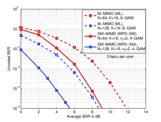
Figure 3: BER performance of multiuser SM-MIMO ($n_{t}=2$, $n_{rf}=1$, 4-QAM) using MPD-SM algorithm and massive MIMO ($n_{t}=1$, $n_{rf}=1$, 8-QAM) with sphere decoding, at 3 bpcu per user, $K=16$, $N=64,128$.

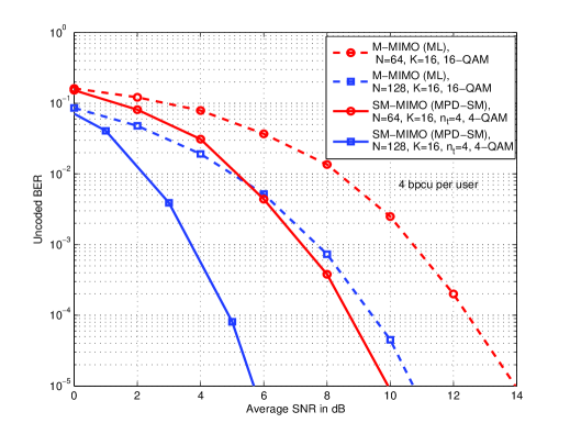
Figure 4: BER performance of multiuser SM-MIMO ($n_{t}=4$, $n_{rf}=1$, 4-QAM) using MPD-SM algorithm and massive MIMO ($n_{t}=1$, $n_{rf}=1$, 16-QAM) with sphere decoding, at 4 bpcu per user, $K=16$, $N=64,128$.

IV Local Search Detection for SM-MIMO

In this section, we propose another algorithm for SM-MIMO detection. The algorithm is based on local search. The algorithm finds a local optimum (in terms of ML cost) as the solution through a local neighborhood search. We refer to this algorithm as LSD-SM (local search detection for spatial modulation) algorithm. A key to the LSD-SM algorithm is the definition of a neighborhood suited for SM. This is important since SM carries information bits in the antenna indices also.

Neighborhood definition: For a given vector ${\bf x}\in{\mathbb{S}}_{n_{t},{\mathbb{A}}}^{K}$, we define the neighborhood ${\cal N}({\bf x})$ to be the set of all vectors in ${\mathbb{S}}_{n_{t},{\mathbb{A}}}^{K}$ that differ from the vector ${\bf x}$ in either one spatial index position or in one modulation symbol. That is, a vector ${\bf w}$ is said to be a neighbor of ${\bf x}$ if and only if ${\bf w}_{k}\in\{{\mathbb{S}}_{n_{t},{\mathbb{A}}}\setminus{\bf x}_{k}\}$ for exactly one $k$, and ${\bf w}_{k}={\bf x}_{k}$ for all other $k$, i.e., the neighborhood ${\cal N}({\bf x})$ is given by

$${\cal N}({\bf x})\triangleq\big{\{}{\bf w}|{\bf w}\in{\mathbb{S}}_{n_{t},{\mathbb{A}}}^{K},{\bf w}_{k}\neq{\bf x}_{k}\text{ for exactly one }k\big{\}},$$ (13)

where ${\bf x}_{k},{\bf w}_{k}\in{\mathbb{S}}_{n_{t},{\mathbb{A}}}$ and $k\in{1,2,\cdots,K}$. Thus the size of this neighborhood is given by $|{\cal N}({\bf x})|=(|{\mathbb{S}}_{n_{t},{\mathbb{A}}}|-1)K$.

For example, consider $K=2$, $n_{t}=2$, and BPSK (i.e., ${\mathbb{A}}=\{\pm 1\}$). We then have

$${\small{\mathbb{S}}_{2,\mbox{\tiny BPSK}}=\Bigg{\{}\begin{bmatrix}+1\\ 0\end{bmatrix},\begin{bmatrix}-1\\ 0\end{bmatrix},\begin{bmatrix}0\\ +1\end{bmatrix},\begin{bmatrix}0\\ -1\end{bmatrix}\Bigg{\}}},$$

and

${\cal N}\left(\begin{bmatrix}+1\\ 0\\ 0\\ -1\end{bmatrix}\right)=\left\{\begin{bmatrix}-1\\ 0\\ 0\\ -1\end{bmatrix},\begin{bmatrix}0\\ +1\\ 0\\ -1\end{bmatrix},\begin{bmatrix}0\\ -1\\ 0\\ -1\end{bmatrix},\begin{bmatrix}-1\\ 0\\ 0\\ +1\end{bmatrix},\begin{bmatrix}-1\\ 0\\ -1\\ 0\end{bmatrix},\begin{bmatrix}-1\\ 0\\ +1\\ 0\end{bmatrix}\right\}$.

LSD-SM algorithm: The LSD-SM algorithm for SM-MIMO detection starts with an initial solution vector $\hat{{\bf x}}^{(0)}$ as the current solution. For example, $\hat{{\bf x}}^{(0)}$ can be the MMSE solution vector $\hat{{\bf x}}_{\tiny{\mbox{MMSE}}}$. Using the neighborhood definition in (13), it considers all the neighbors of $\hat{{\bf x}}^{(0)}$ and searches for the best neighbor with least ML cost which also has a lesser ML cost than the current solution. If such a neighbor is found, then it declares this neighbor as the current solution. This completes one iteration of the algorithm. This process is repeated for multiple iterations till a local minimum is reached (i.e., no neighbor better than the current solution is found). The vector corresponding to the local minimum is declared as the final output vector ${\hat{\bf x}}$. The non-zero entry in the $k$th user’s sub-vector in ${\hat{\bf x}}$ and its index are then demapped to obtain the information bits of the $k$th user.

Multiple restarts: The performance of the basic LSD-SM algorithm in the above can be further improved by using multiple restarts, where the LSD-SM algorithm is run several times, each time starting with a different initial solution and declaring the best solution among the multiple runs. The proposed LSD-SM algorithm with multiple restarts is listed in Algorithm 2.

1:  $\mathbf{Input:y,H}$, $r$: no. of restarts

2:  for $j$ = 1 to $r$  do

3:     compute $\mathbf{c}^{(j)}$  (initial vector at $j$th restart)

4:     find $\mathcal{N}(\mathbf{c}^{(j)})$

5:     $\mathbf{z}^{(j)}$ = $\underset{\mathbf{q}\in\mathcal{N}(\mathbf{c}^{(j)})}{\mathrm{argmin}}~{}\|\mathbf{y-Hq}\|^{2}$

6:     if  $\|\mathbf{y-H\mathbf{z}}^{(j)}\|^{2}<\|\mathbf{y-H\mathbf{c}}^{(j)}\|^{2}$  then

7:        $\mathbf{c}^{(j)}$ = $\mathbf{z}^{(j)}$

8:        goto step 4

9:     else

10:        $\hat{\mathbf{x}}^{(j)}$ = $\mathbf{c}^{(j)}$

11:     end if

12:  end for

13:  $i$ = $\underset{1\leq j\leq r}{\mathrm{argmin}}\ \|\mathbf{y-H}\hat{\mathbf{x}}^{(j)}\|^{2}$

14:  $\mathbf{Output}$ : ${\hat{\bf x}}=\hat{\mathbf{x}}^{(i)}$

Algorithm 2 Listing of the proposed LSD-SM algorithm with multiple restarts.

Complexity: The LSD-SM algorithm complexity consists of two parts. The first part involves the computation of the initial solution. The complexity for computing the MMSE initial solution is $\mathcal{O}(Kn_{t}N^{2})$. The second part involves the search complexity, where, in order to compute the ML cost, we require to compute $(i)$ ${\bf H}^{H}{\bf H}$ which has $\mathcal{O}(K^{2}n_{t}^{2}N)$ complexity, and $(ii)$ ${\bf H}^{H}{\bf y}$ which has $\mathcal{O}(Kn_{t}N)$ complexity. In addition, the complexity per iteration and the number of iterations to reach the local minima contribute to the search complexity, where the search complexity per iteration is $O(K|{\mathbb{S}}_{n_{t},{\mathbb{A}}}|)$.

Reducing the search complexity: From the above discussion on the complexity of the LSD-SM algorithm, we saw that the computation of the ML cost requires a complexity of order $O(K^{2}n_{t}^{2}N)$ which is greater than the MMSE complexity of $O(Kn_{t}N^{2})$ for systems with $Kn_{t}>N$, i.e., with loading factor $\alpha>1/n_{t}$. We propose to reduce the search complexity by the following method, which consists of the following three parts:

1. The channel gain matrix ${\bf H}$ can be written as ${\bf H}=[{\bf h}_{1}\ {\bf h}_{2}\ \cdots\ {\bf h}_{Kn_{t}}]$, where ${\bf h}_{i}$ is the $i$th column of ${\bf H}$, which is a $N\times 1$ column vector. Before we start the search process in the LSD-SM algorithm, compute the set of vectors $\mathbb{J}\triangleq\{{\bf h}_{i}s\}_{\forall s\in{\mathbb{A}},\forall i\in 1,2,\cdots,Kn_{t}}$. The complexity of this computation is $O(|{\mathbb{A}}|Kn_{t}N)$.

2. Compute the vector ${\bf z}^{(0)}$, which is defined as

   $${\bf z}^{(0)}\triangleq{\bf y}-{\bf H}\hat{{\bf x}}^{(0)}={\bf y}-\sum_{k=1}^{K}\hat{x}^{(0)}_{l_{k}}{\bf h}_{(k-1)n_{t}+j_{k}},$$ (14)

   where the terms $\hat{x}^{(0)}_{l_{k}}{\bf h}_{(k-1)n_{t}+j_{k}}$ belong to $\mathbb{J}$ which is precomputed. The computation of ${\bf z}^{(0)}$ requires a complexity of $O(KN)$.

3. Because of the way the neighborhood is defined, every neighbor of ${\bf z}^{(0)}$ can be computed from ${\bf z}^{(0)}$ by exactly adding a single vector from $\mathbb{J}$ and subtracting another vector from $\mathbb{J}$. Thus the complexity of computing the ML cost of every neighbor is $O(N)$.

In this method, the total number of operations performed for the search is $|{\mathbb{A}}|Kn_{t}N+K(N+1)+(2N-1)+K(|{\mathbb{A}}|n_{t}-1)(4N-1)T$, where $T$ is the number of iterations performed to reach the local minima which depends on the transmit vector and the operating SNR ($T$ is determined through simulations). Therefore, the total complexity of the algorithm in this method is given by $O(|{\mathbb{A}}|Kn_{t}NT)$, whereas, the total complexity without search complexity reduction is $O(K^{2}n_{t}^{2}N)$.

Performance: We evaluated the performance of multiuser SM-MIMO using the proposed LSD-SM algorithm and compared it with that of massive MIMO using ML detection for the same spectral efficiency. Figure 5 shows the performance comparison between SM-MIMO with ($n_{t}=4$, 4-QAM) and massive MIMO with ($n_{t}=1$, 16-QAM), both having 4 bpcu per user. For SM-MIMO, detection performance of both LSD-SM (presented in this section) and MPD-SM (presented in the previous section) are shown. In LSD-SM, the number of restarts used is $r=2$. The initial vectors used in the first and second restarts are MMSE solution vector and random vector, respectively. For massive MIMO, ML detection performance using sphere decoder is plotted. It can be seen that SM-MIMO using LSD-SM and MPD-SM algorithms outperform massive MIMO using sphere decoding. Specifically, SM-MIMO using LSD-SM performs better than massive MIMO by about 5 dB at $10^{-3}$ BER. Also, comparing the performance of LSD-SM and MPD-SM algorithms in SM-MIMO, we see that LSD-SM performs better than MPD-SM by about 1 dB at $10^{-3}$ BER.

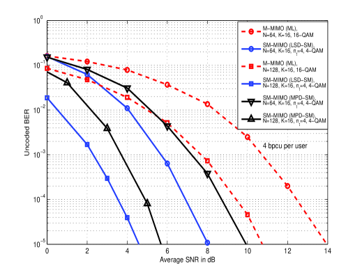
Figure 5: BER performance of multiuser SM-MIMO ($n_{t}=4$, $n_{rf}=1$, 4-QAM) using LSD-SM and MPD-SM algorithms, and massive MIMO ($n_{t}=1$, $n_{rf}=1$, 16-QAM) using sphere decoding, at 4 bpcu per user, $K=16$, $N=64,128$.

Hybrid MPD-LSD-SM detection: The LSD-SM algorithm proposed in this section offers good performance but has higher complexity due to the requirement of the initial MMSE solution vector. The high complexity of MMSE is due to the need for matrix inversion. We can overcome this need for MMSE computation by using a hybrid detection scheme. In the hybrid detection scheme, we first run the MPD-SM algorithm (proposed in the previous section) and the output of the MPD-SM algorithm is fed as the initial solution vector to the LSD-SM algorithm (proposed in this section). We refer to this hybrid scheme as the ‘MPD-LSD-SM’ scheme. The MPD-LSD-SM scheme does not need the MMSE solution and hence avoids the associated matrix inversion.

Performance as a function of loading factor: In Fig. 6, we compare the performance of SM-MIMO (with $n_{t}=4$, $n_{rf}=1$, 4-QAM) and massive MIMO (with $n_{t}=n_{rf}=1$, 16-QAM), both at 4 bpcu per user, as a function of system loading factor $\alpha$, at an average SNR of 9 dB. For SM-MIMO, the detectors considered are MMSE, MPD-SM, LSD-SM, and the hybrid MPD-LSD-SM. The detectors considered for massive MIMO are MMSE detector and MMSE-LAS detector in [1],[2] with 2 restarts. From Fig 6, we observe that SM-MIMO performs significantly better than massive MIMO at low to moderate loading factors. For the same SM-MIMO system settings, we show the complexity plots for various SM-MIMO detectors at different loading factors in Fig. 7. It can be seen that the proposed MPD-SM detector has less complexity than MMSE detector; yet, MPD-SM detector outperforms MMSE detector (as can be seen in Fig. 6). The proposed LSD-SM detector performs better than the MPD-SM detector with some additional computational complexity (as can be seen in Fig. 7). Among the considered detection schemes, the hybrid MPD-LSD-SM detection scheme gives the best performance with near-MMSE complexity.

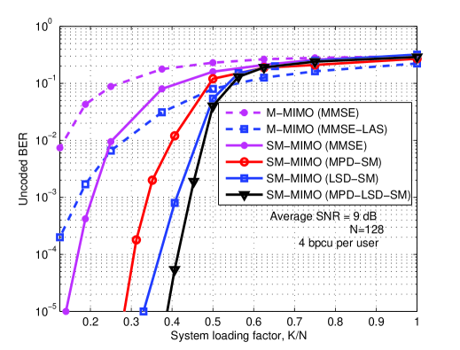
Figure 6: BER performance of SM-MIMO ($n_{t}=4$, $n_{rf}=1$, 4-QAM) and massive MIMO ($n_{t}=1$, $n_{rf}=1$, 16-QAM) as a function of system loading factor, $\alpha$. $N=128$, SNR = 9 dB, and 4 bpcu per user.

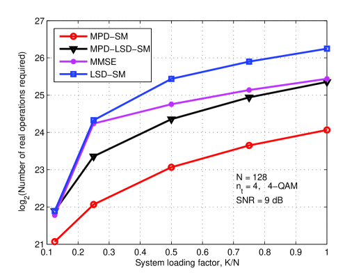
Figure 7: Complexity comparison between MMSE, MPD-SM, LSD-SM and hybrid MPD-LSD-SM detection algorithms in multiuser SM-MIMO as a function of system loading factor, $\alpha$. $N=128$, $n_{t}=4$, $n_{rf}=1$, 4-QAM, 4 bpcu per user and SNR = 9 dB.

Performance for same spectral efficiency and QAM size: We note that if both spectral efficiency and QAM size are to be kept same in SM-MIMO and massive MIMO, then the number of spatial streams per user in massive MIMO has to increase. For example, SM-MIMO can achieve 4 bpcu per user with 4-QAM using $n_{t}=4$ and $n_{rf}=1$. Massive MIMO can achieve the same spectral efficiency of 4 bpcu per user using one spatial stream (i.e., $n_{t}=n_{rf}=1$) with 16-QAM. But to achieve the same spectral efficiency using 4-QAM in massive MIMO, we have to use $n_{t}=n_{rf}=2$, i.e., two spatial streams per user with 4-QAM on each stream are needed. This increase in number of spatial streams per user increases the spatial interference.

The effect of increase in number of spatial streams per user in massive MIMO for the same spectral efficiency on the performance is illustrated in Fig. 8 for $K=16$ and $N=128$. In Fig. 8, we compare the performance of the following four systems with the same spectral efficiency of 4 bpcu per user: 1) SM-MIMO with ($n_{t}=4$, $n_{rf}=1$, 4-QAM), 2) massive MIMO with ($n_{t}=n_{rf}=1$, 16-QAM), 3) massive MIMO with ($n_{t}=n_{rf}=2$, 4-QAM), and 4) massive MIMO with ($n_{t}=n_{rf}=4$, BPSK). It can be seen that among the four systems considered in Fig. 8, SM-MIMO performs the best. This is because massive MIMO loses performance because of higher-order QAM or increased spatial interference from increased number of spatial streams per user.

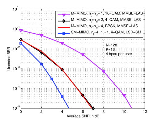
Figure 8: BER performance of SM-MIMO with ($n_{t}=4$, $n_{rf}=1$, 4-QAM), massive MIMO with ($n_{t}=n_{rf}=1$, 16-QAM), massive MIMO with ($n_{t}=n_{rf}=2$, 4-QAM), and massive MIMO with ($n_{t}=n_{rf}=4$, BPSK) for $K=16$, $N=128$, 4 bpcu per user.

V Conclusions

We proposed low complexity detection algorithms for large-scale SM-MIMO systems. These algorithms, based on message passing and local search, scaled well in complexity and achieved very good performance. An interesting observation from the simulation results is that SM-MIMO outperforms massive MIMO by several dBs for the same spectral efficiency. The SNR advantage of SM-MIMO over massive MIMO is attributed to the following reasons: $(i)$ because of the spatial index bits, SM-MIMO can use a lower-order QAM alphabet compared to that in massive MIMO to achieve the same spectral efficiency, and $(ii)$ for the same spectral efficiency and QAM size, massive MIMO will need more spatial streams per user which leads to increased spatial interference. With such performance advantage at low RF hardware complexity, large-scale multiuser SM-MIMO is an attractive technology for next generation wireless systems and standards like 5G and HEW (high efficiency WiFi).

References

- [1] K. V. Vardhan, S. K. Mohammed, A. Chockalingam, and B. S. Rajan, “A low-complexity detector for large MIMO systems and multicarrier CDMA systems,” IEEE J. Sel. Areas Commun., vol. 26, no. 3, pp. 473-485, Apr. 2008.
- [2] S. K. Mohammed, A. Zaki, A. Chockalingam, and B. S. Rajan, “High-rate space–time coded large-MIMO systems: low-complexity detection and channel estimation,” IEEE J. Sel. Topics Signal Proc., vol. 3, no. 6, pp. 958-974, Dec. 2009.
- [3] F. Rusek, D. Persson, B. K. Lau, E. G. Larsson, T. L. Marzetta, O. Edfors, and F. Tufvesson, “Scaling up MIMO: opportunities and challenges with very large arrays,” IEEE Signal Process. Mag., vol. 30, no. 1, pp. 40-60, Jan. 2013.
- [4] J. Hoydis, S. ten Brink, and M. Debbah, “Massive MIMO in the UL/DL of cellular networks: how many antennas do we need?” IEEE J. Sel. Areas in Commun., vol. 31, no. 2, pp. 160-171, Feb. 2013.
- [5] M. Di Renzo, H. Haas, and P. M. Grant, “Spatial modulation for multiple-antenna wireless systems: a survey,” IEEE Commun. Mag., vol. 50, no. 12, pp. 182-191, Dec. 2011.
- [6] M. Di Renzo, H. Haas, A. Ghrayeb, S. Sugiura, and L. Hanzo, “Spatial modulation for generalized MIMO: challenges, opportunities and implementation,” Proceedings of the IEEE. [Online]. Available: http://eprints.soton.ac.uk/354175/
- [7] N. Serafimovski1, S. Sinanovic, M. Di Renzo, and H. Haas, “Multiple access spatial modulation,” EURASIP J. Wireless Commun. and Networking 2012, 2012:299.
- [8] N. Serafimovski, S. Sinanovic, A. Younis, M. Di Renzo, and H. Haas, “2-user multiple access spatial modulation,” Proc. IEEE HeterWMN’2011, Dec. 2011.
- [9] M. Di Renzo and H. Haas, “Bit error probability of space-shift keying MIMO over multiple-access independent fading channels,” IEEE Trans. Veh. Tech., vol. 60, no. 8, pp. 3694-3711, Oct. 2011.
- [10] M. Pretti, “A message passing algorithm with damping,” J. Stat. Mech.: Theory and Practice, Nov. 2005, P11008.