Secular chaos and its application to Mercury, hot Jupiters, and the organization of planetary systems

Abstract

In the inner solar system, the planets’ orbits evolve chaotically, driven primarily by secular chaos. Mercury has a particularly chaotic orbit, and is in danger of being lost within a few billion years. Just as secular chaos is reorganizing the solar system today, so it has likely helped organize it in the past. We suggest that extrasolar planetary systems are also organized to a large extent by secular chaos. A hot Jupiter could be the end state of a secularly chaotic planetary system reminiscent of the solar system. But in the case of the hot Jupiter, the innermost planet was Jupiter- (rather than Mercury-) sized, and its chaotic evolution was terminated when it was tidally captured by its star. In this contribution, we review our recent work elucidating the physics of secular chaos and applying it to Mercury and to hot Jupiters. We also present new results comparing the inclinations of hot Jupiters thus produced with observations.

1 Introduction

The question of the stability of the solar system has a long and illustrious history (e.g., [1]). It was finally answered with the aid of computer simulations [2, 3, 4], which have shown that the solar system is marginally stable: it is chaotically unstable, but on a timescale comparable to its age. In the inner solar system, the planets’ eccentricities ($e$) and inclinations ($i$) diffuse in billions of years, with the two lightest planets, Mercury (Fig. 1) and Mars, experiencing particularly large variations. Mercury may even be lost from the solar system on a billion-year timescale [5, 6, 7]. Yet despite the spectacular success in solving solar system stability, fundamental questions remain: What is the theoretical explanation for orbital chaos of the solar system? What does the chaotic nature of the solar system teach us about its history and organization? And how does this relate to extrasolar systems?

For well-spaced planets that are not close to strong mean-motion-resonances (MMR’s), the orbits evolve on timescales much longer than orbital periods. Hence one may often simplify the problem by orbit-averaging the interplanetary interactions. The averaged equations are known as the secular equations (e.g., [11]). To linear order in masses, secular evolution consists of interactions between rings, which represent the planets after their masses have been smeared out over an orbit. Secular evolution dominates the evolution of the terrestrial planets in the solar system [5], and it is natural to suppose that it dominates in many extrasolar systems as well. This is the type of planetary interaction we focus on in this contribution.

One might be tempted by the small eccentricities and inclinations in the solar system to simplify further and linearize the secular equations, i.e., consider only terms to leading order in eccentricity and inclination. Linear secular theory reduces to a simple eigenvalue problem. For $N$ secularly interacting planets, the solution consists of $2N$ eigenmodes: $N$ for the eccentricity degrees of freedom and another $N$ for the inclination. Each of the eigenmodes evolves independently of the others [11]. Linear secular theory provides a satisfactory description of the planets’ orbits on million year timescales. It is the cause, for example, of Earth’s eccentricity-driven Milankovitch cycle. But on timescales $\gtrsim 10^{7}$ years, the evolution is chaotic (e.g., Fig. 1), in sharp contrast to the prediction of linear secular theory. That appears to be puzzling, given the small eccentricities and inclinations in the solar system.

Yet despite its importance, there has been little theoretical understanding of how secular chaos works. Conversely, chaos driven by MMR’s is much better understood. For example, chaos due to MMR overlap explains the Kirkwood gaps in the asteroid belt [12], and chaos due to the overlap of 3-body MMR’s accounts for the very weak chaos in the outer solar system [8]. Since chaos in the solar system is typically driven by overlapping resonances (e.g., see review [13]), one might reason that the secular chaos of the inner solar system is driven by overlapping secular resonances. Laskar and Sussman & Wisdom [14, 15, 16] identified a number of candidate secular resonances that might drive chaos in the inner solar system by examining angle combinations that alternately librated and circulated in their simulations. But there are an infinite number of such angle combinations, and it is not clear which are dynamically important—or why [16, 13].

In [17] (hereafter LW11) we developed the theory for secular chaos, and applied it to Mercury, the solar system’s most unstable planet. We demonstrated how the locations and widths of general secular resonances can be calculated, and how the overlap of the relevant resonances quantitatively explains Mercury’s chaotic orbit. This theory, which we review below, shows why Mercury’s motion is nonlinear—and chaotic—even though $e$’s and $i$’s remain modest. It also shows that Mercury lies just above the threshold for chaotic diffusion.

A system of just two secularly interacting planets can be chaotic if their eccentricities and inclinations are both of order unity [18, 19, 20]. In systems with three or more planets, on the other hand, there is a less stringent criterion on the minimum eccentricity and inclination required for chaos, and the character of secular chaos is more diffusive. This diffusive type of secular chaos promotes equipartition between different secular degrees of freedom. During secular chaos, the angular momentum of each planet varies chaotically, with the innermost planet being slightly more susceptible to large variations ([21], hereafter WL11). If enough angular momentum is removed from that planet, its pericenter will approach the star. And if that planet resembles Jupiter, tidal interaction with its host star may then remove its orbital energy, turning it into a hot Jupiter. Hot Saturns or hot Neptunes may also be produced similarly. As shown in WL11 and reviewed below, such a migration mechanism can reproduce a range of observed features of hot Jupiters, giant planets that orbit their host stars at periods of a few days. It differs from other mechanisms that have been proposed for migrating hot Jupiters, including disk migration [33, 34], planet scattering [37], and Kozai migration by a stellar or planetary companion [35, 36, 20].

These studies prompt us to suggest that secular chaos may play an important role in reshaping planetary systems after they emerge from their nascent disks. Secular chaos causes planets’ eccentricities to randomly wander. When one of the planets attains high enough $e$ that it suffers collision, ejection, or tidal capture, the removal of that planet can then lead to a more stable system, with a longer chaotic diffusion time. Such a scenario (e.g., [1]) can explain why the solar system, as well as many observed exo-planetary systems, are perched on the threshold of instability.

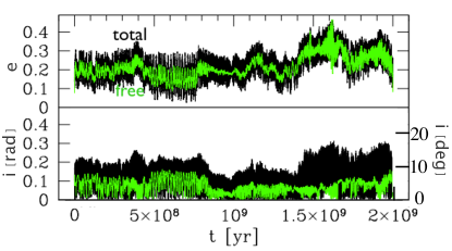
Figure 1: Mercury’s chaos in an N-body integration of the solar system. Black shows Mercury’s total eccentricity and inclination. Green shows free $e$ and $i$, which were obtained by filtering out the forcing frequencies of the other planets in Fourier space. The wander of the green curves demonstrates that Mercury’s orbit is chaotic. Adapted from LW11.

2 Theory of Secular Chaos

2.1 Linear Secular Theory

We review first linear secular theory before introducing nonlinear effects. The equations of motion may be derived from the expression for the energy, which we shall label $H$ because it turns into the Hamiltonian after replacing orbital elements with canonical variables. Focusing first on two coplanar planets, their secular interaction energy is, to leading order in eccentricities and dropping constant terms,

$$H=-G{mm^{\prime}\over a^{\prime}}\left(f_{2}(e^{2}+e^{\prime 2})+f_{10}ee^{\prime}\cos\left({\varpi-\varpi^{\prime}}\right)\right)\ ,$$ (1)

following the notation of [11] and dropping higher order terms in $e$ (which lead to nonlinear equations). Here, unprimed and primed quantities denote the inner and outer planets and $f_{j}$ are Laplace coefficients that are functions of $\alpha\equiv a/a^{\prime}$ (Appendix B in [11]). In secular theory the semimajor axes are constant (even to nonlinear order), and hence may be considered as parameters. To derive the equations of motion for the inner planet, one replaces $e$ and $\varpi$ in the interaction energy with a canonically conjugate pair (e.g., the Poincaré variables $\Gamma\approx m({GM_{*}a})^{1/2}e^{2}/2$ and $\gamma=-\varpi$) and employs the usual Hamilton’s equations for $\Gamma$ and $\gamma$. The same is true for the outer planet. One finds, after writing the resulting equations in terms of complex eccentricities ($z\equiv ee^{i\varpi}$ and $z^{\prime}\equiv e^{\prime}e^{i\varpi^{\prime}}$)

$${d\over dt}\left(\begin{array}[]{c}z\\ z^{\prime}\end{array}\right)=i{2f_{2}n^{\prime}\over\sqrt{a}}\left(\begin{array}[]{cc}\mu^{\prime}\sqrt{a^{\prime}}&-\beta\mu^{\prime}\sqrt{a^{\prime}}\\ -\beta\mu\sqrt{a}&\mu\sqrt{a}\end{array}\right)\left(\begin{array}[]{c}z\\ z^{\prime}\end{array}\right)$$ (8)

where $n^{\prime}=\sqrt{GM_{*}/a^{\prime 3}}$, $\mu=m/M_{*}$, and $\beta=-f_{10}/(2f_{2})$ (For example, $\beta\approx 5\alpha/4$ for small $\alpha$.) The solution to this linear set of equations is a sum of two eigenmodes, each of which has a constant amplitude and a longitude that precesses uniformly in time. The theory may be trivially extended to $N$ planets, leading to $N$ eigenmodes. It may also be extended to linear order in inclinations, which leads to a second set of $N$ eigenmodes. The equations for $\zeta=ie^{i\Omega}$ are identical to those for $z$, but with $\beta\rightarrow 1$.

2.2 Overlap of Secular Resonances Drives Secular Chaos

The linear equations admit the possibility for a secular resonance, which occurs when two eigenfrequencies match. Consider a massless particle perturbed by a precessing mode. In anticipation of application to the solar system, one may think of the test particle as Mercury, and the mode as the one dominated by Jupiter. Equation (8) implies that the particle’s $z$ is governed by

$${dz\over dt}=i\gamma\left(z-e_{m}e^{ig_{m}t}\right)\ ,$$ (9)

where $\gamma$ is the particle’s free precession rate, $g_{m}$ is the mode’s precession rate, and $e_{m}$ is proportional to the mode’s amplitude (i.e., to the eccentricities of the massive planets that participate in the mode). To order of magnitude, $\gamma\sim n\mu_{*}\alpha_{*}^{3}$ and $e_{m}\sim\alpha_{*}e_{*}$, where starred quantities correspond to the planets that dominate the forcing (and assuming $\alpha_{*}\ll 1$). The solution to equation (9) is a sum of free and forced eccentricities:

$$z={\rm const}\times e^{i\gamma t}+e_{m}{\gamma\over\gamma-g_{m}}e^{ig_{m}t}\ .$$ (10)

The free eccentricity exists even in the absence of the mode, and it precess at frequency $\gamma$. The forced eccentricity precesses at the frequency of the mode that drives it, and its amplitude is proportional to that mode’s amplitude. Formally, it diverges at resonance, $\gamma=g_{m}$. But nonlinearities alter that conclusion.

The leading nonlinear correction to Hamiltonian (1) is fourth order in eccentricity, which changes Equation (9) to.

$${dz\over dt}=i\gamma\left(z\left(1-{|z|^{2}\over 2}\right)-e_{m}e^{ig_{m}t}\right)\$$ (11)

Hence nonlinearity reduces the frequency of free precession from $\gamma$ to $\gamma(1-e^{2}/2)$. There are a number of interesting consequences. First, even if the particle is at exact linear resonance ($\gamma=g_{m}$), then as its eccentricity changes its frequency shifts away from resonance, protecting it against the divergence that appears in linear theory (eq. 10). Second, if the particle is not at linear resonance it can still approach resonance when its eccentricity changes. With nonlinearity included, a resonance takes on the familiar shape of a “cat’s eye” in phase space, and a particle can librate stably in resonance (Fig. 1 of LW11).

Although the nonlinear cat’s eye protects against divergences, danger lurks at the corner of a cat’s eye: an unstable fixed point. Motion due to a single resonance (e.g., Eq. 11) is perfectly regular (non-chaotic). But if there is a second resonance nearby in phase space—in particular, if the separatrices enclosing two different cats’ eyes overlap—chaos ensues (Fig 2 of LW11). Chaos due to the overlapping of resonances drives Mercury’s long-term evolution, and may well be one of the key drivers of the long-term evolution of planetary systems.

3 Mercury

The theory described above for coplanar secular chaos was first developed by [22]. But to explain secular chaos in the solar system, one must extend it to include non-zero inclinations, which we did in LW11. Mercury has two free frequencies, one for its eccentricity ($z$) and one for its inclination ($\zeta$). We denote these $g$ and $s$ respectively. In linear theory, $g=-s=\gamma$. But to leading nonlinear order, these frequencies are modified in the manner described above to

$$g = \gamma\left(1-{e^{2}\over 2}-2i^{2}\right)$$ (12)

$$s = \gamma\left(-1-2e^{2}+{i^{2}\over 2}\right)$$ (13)

(LW11). Each of these frequencies can be in resonance with one of the other 13 planetary modes—2 for each planet, excluding the zero frequency inclination mode that defines the invariable plane. Two solar system modes have frequencies close to Mercury’s linear eccentricity precession rate (i.e., to $\gamma$): the Venus-dominated $e$-mode (frequency $g_{2}$) and the Jupiter-dominated $e$-mode ($g_{5}$). And one mode’s frequency lies close to Mercury’s linear inclination precession rate (i.e., to $-\gamma$): the Venus-dominated $i$-mode ($s_{2}$). One can visualize this by imagining moving Mercury’s $a$, holding its $e=i=0$. Since $\gamma$ is a function of $a$, the linear secular resonances occur at particular values of $a$. The three aforementioned resonances lie $\sim 20\%$ away from Mercury’s actual $a$ at $e=i=0$ (Fig. 2). Since Mercury is at some distance from those resonances to linear order, it is at first sight surprising that they can play an important role in Mercury’s evolution. But Equations (12)–(13) show that the locations of these resonances move as Mercury’s $e$ and $i$ are increased. In fact, two of them ($g_{5}$ and $s_{2}$) overlap very close to Mercury’s current orbital parameters. The overlapping of those two resonances is the underlying cause of Mercury’s chaos. Even though Mercury has relatively small $e$ and $i$, its proximity to two secular resonances drives its orbit to be chaotic.

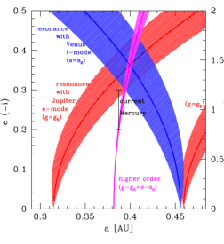
Figure 2: Secular resonances that lead to Mercury’s orbital chaos, showing that Mercury’s current orbit is close to the overlap of two secular resonances (i.e., $g=g_{5}$ with $s=s_{2}$). To plot the lines at the center of these resonances we assume the current values of $g_{5}$ and $s_{2}$, and that Mercury remains with $e=i$. The widths of the resonances, as calculated in LW11, are shaded. The widths depend not only on Mercury’s orbital parameters, but on the other planets’ as well. To plot these widths, we scale all of the planets’ $e$’s and $i$’s by the same factor ($\kappa$; see right axis) relative to their current values. We do this to illustrate how the solar system is perched on the threshold of chaos. For this plot, the widths are only correct within a factor of $\lesssim 2$ because the exact width (see LW11) depends on the trajectory of an orbit in $e$-$i$ space.

To make the above theory more precise, one must calculate the widths of the resonances, which are sketched in Figure 2. If the resonant widths are negligibly small, Mercury would have to lie precisely at the region of overlap, which would be unlikely. One also has to account for higher order (combinatorial) resonances, the most important one of which is $(g-g_{5})-(s-s_{2})$. That combinatorial resonance was identified by Laskar [14] from the fact that it librated in his simulations for 200 Myr. In LW11, we calculated the widths of the aforementioned resonances, and showed that the widths match in detail what is seen in simulations (see Figs. 4, 6, and 7 in that paper).

Figure 3 compares Mercury’s orbital evolution in an N-body simulation of the solar system (blue points) with the prediction based on a simplified model that includes only the $g_{5}$ and $s_{2}$ forcing terms. Mercury’s true orbit traces the boundary of chaos as predicted by the model, illustrating that the model suffices to explain Mercury’s chaos. More dramatically, it also illustrates how Mercury is perched on the threshold of chaos. We speculate below as to how Mercury might have ended up in such a seemingly unlikely state.

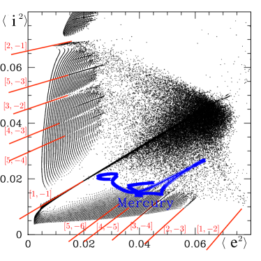
Figure 3: The blue points show the running average of Mercury’s $e^{2}$ and $i^{2}$ in an N-body simulation of the solar system that lasts 600 Myr. The black points illustrate where chaos occurs in a highly simplified model that includes only the $g_{5}$ and $s_{2}$ forcing frequenices. Those points denote the time-averaged results from simulations that are initialized on a regular grid; hence the regularly spaced black points denote non-chaotic orbits, and the irregularly spaced points denote chaotic ones. The fact that Mercury’s orbit lies within the chaotic zone shows that our highly simplified model is sufficient to account for Mercury’s chaos. Moreover, this model demonstrates that Mercury is perched on the threshold of chaos. The red lines denote various secular resonances that involve the $g_{5}$ and $s_{2}$ frequencies. Adapted from Fig. 5 of LW11; see that paper for more detail.

4 Hot Jupiters

The first batch of extra-solar planets that were discovered were “hot Jupiters” [23, 24]. It is now clear that $\sim 1\%$ of solar-type stars are orbited by jovian giant planets with periods of $\sim 3$ days. In comparison with this pile-up of hot Jupiters at small separation [25, 26, 27, 28], there is a deficit of gas giants with periods between $10$ and $100$ days (the “period valley;” [29, 30]) before the number picks up and rises outward again (see reviews [31, 32]).

According to conventional theories of planet formation, hot Jupiters could not have formed in situ, given the large stellar tidal field, high gas temperature, and low disk mass to be found so close to the star. It is therefore commonly thought that these planets are formed beyond a few AU and then are migrated inward. Candidate migration scenarios that have been proposed include protoplanetary disks (e.g., [33, 34]), Kozai migration by binary or planetary companions (e.g., [35, 36, 20]), scattering with other planets in the system (e.g., [37]), and secular chaos [21, 38]. A critical review of these mechanisms is given in WL11.

Here we present a short description of the secular chaos scenario. Moreover, now that the orbital axis (relative to the stellar rotation axis) of some $60$ hot Jupiters has been measured, we compare the observed distribution against that produced in a new suite of secular chaos simulations.

4.1 Simulations and Results

Our fiducial planetary system is composed of three giant planets ($0.5,1.0,1.5M_{J}$) that are well-spaced ($1,6,16$ AU) with initially mild eccentricities and inclinations ($e=0.07$ to $0.3$, inclination $4.5$ to $20^{\circ}$, see Table 1 of WL11). Such a configuration is possible for a system that emerges out of a dissipative proto-planetary disk, as it avoids short-term instabilities. But disk-planet interactions are not yet well understood. It is also possible that disks always damp planets onto nearly circular coplanar orbits, in which case such $e$’s and $i$’s might arise from, e.g., planet scattering or collisions.

The angular momentum deficit is defined as (e.g., [39, 40] )

$${\rm AMD}\equiv\sum_{k}m_{k}\sqrt{a_{k}}(1-\sqrt{1-e_{k}^{2}}\cos i_{k})\approx\sum_{k}{1\over 2}m_{k}\sqrt{a_{k}}(e_{k}^{2}+i_{k}^{2})\,,$$ (14)

where the summation is over all planets. The AMD describes the deficit in angular momentum relative to that of a coplanar, circular system. When the AMD is not zero, secular interactions continuously modify the planets’ eccentricities and inclinations, preserving the total AMD (since the total angular momentum is conserved, and secular interactions do not modify the orbital energies). A system with a higher AMD will interact more strongly, and above some critical AMD value, the evolution is chaotic (e.g., Fig. 2). In order to produce a hot Jupiter by secular interactions (requring that $e_{1}\rightarrow 1$), the minimum AMD value is ${\rm AMD}=m_{1}\sqrt{a_{1}}$. Our fiducial system has an AMD of $1.17m_{1}\sqrt{a_{1}}$. This AMD value is also high enough for the system to be secularly chaotic.

In Figure 4, we observe that the three planets secularly (and diffusively) transfer angular momentum (but not energy) for almost 300 Myrs without major mishap, until the inner planet has gradually acquired so much AMD that its eccentricity, starting at $e_{1}=0.07$, has reached $e_{1}=0.985$. This corresponds to a periapse distance of order the Roche radius, $a(1-e)$ $\sim$$0.015$AU. We then specify in our numerical simulation that tidal interaction with the central star removes orbital energy from the planet [41]. The orbit decays inward, until the planet is tidally circularized at $\sim 2\times$ Roche radius (because of angular momentum conservation). The inner planet is now captured into a ‘hot Jupiter’.

Since the AMD is transferred to the inner planet to raise its eccentricity, the outer two planets end up with reduced eccentricities and mutual inclinations. They remain at large separations, waiting to be probed by techniques such as radial velocity, astrometry or gravitational lensing. By getting rid of their inner companion the remaining planets organize themselves into a more stable configuration, analogous to what would happen in the inner Solar system after the loss of Mercury.

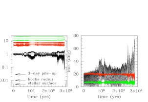
Figure 4: Formation of a hot Jupiter in our fiducial system, simulated using the SWIFT code [42] with tidal and GR effects added. Left: radial excursions of the three planets (semimajor axis, periapse and apoapse) are shown as functions of time, with the various radii relevant for hot Jupiters marked by arrows; right: planet inclinations measured relative to the system’s invariable plane. All planets initially have mildly eccentric and inclined orbits, but over a period of $300$ Myr so much of the angular momentum in the innermost planet can be removed that its eccentricity and inclination can diffusively reach order unity values. The semimajor axes remain nearly constant until the end, a tell-tale sign that secular interactions dominate the dynamics. At $\sim 300$ Myr, the pericenter of the inner planet reaches inward of a few stellar radii and tidal interaction with the central star kicks in. Precessions by general relativity, by tidal and rotational quadrupoles, as well as tidal dissipation, prevent the pericenter from reaching inward of the Roche radius. As a result, the final hot Jupiter has a period of $\sim 3$ days. Adapted from WL11.

In addition to the showcase in Fig. 4, we have performed for this contribution 100 simulations with AMD$=1.5m_{1}\sqrt{a_{1}}$, $50\%$ over the minimum criterion. The planets were initially at 3, 15 and $a_{3}$ AU, with $a_{3}$ uniformly distributed between $30$ and $60$ AU. We find that roughly $60\%$ of these systems produce a hot Jupiter. Most of these newly formed Jupiters have orbits that are prograde relative to the original orbital plane, but some can be retrograde (Fig. 5—to be discussed in more detail below). Moreover, the time for secular chaos to excite the orbital eccentricities to tidal capture ranges from a few million years to a hundred-million years. Raising the initial AMD leads to more efficient hot Jupiter formation.

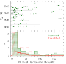
Figure 5: The upper panel shows the sky-projected spin-orbit angles (in absolute value) for some $60$ hot Jupiters ($m\sin i\geq 0.3M_{J}$, data taken from exoplanets.org) as a function of host star effective temperatures. The lower panel shows the distribution of this projected angle (green shaded histogram). The two red histograms show the angle distribution obtained from our simulations before projection (unshaded) and after projection (shaded). Secular chaos tends to produce prograde hot Jupiters, with the projected obliquities peaking at alignment, and a significant tail extending to $\sim 50^{\circ}$.

4.2 Secular Chaos Confronting Observations

In the following, we compare the predictions of secular chaos with observations, highlighting the distribution of spin-orbit angles.

There is a sharp inner cut-off to the 3-day pile-up of hot Jupiters. They appear to avoid the region inward of twice the Roche radius [43], where the Roche radius is the distance within which a planet would be tidally shredded. New data spanning two orders of magnitude in planetary masses (and including planet radius measurements) have strengthened this claim. There are only 5 known exceptions lying inward of twice the Roche radius, and the rest mostly lie between twice and four times the Roche radius. Mechanisms that rely on eccentricity excitation, such as Kozai migration or planet-planet scattering, naturally produce hot Jupiters that tend to avoid the region inside of twice the Roche radius [43]. However, only Kozai migration and secular chaos naturally produce a pile-up just outside twice the Roche radius, as the eccentricity rise in these cases is gradual and planets are accumulated at the right location.

Hot Jupiters appear to be less massive than more distant planets [44, 45, 46]. Among planets discovered with the radial velocity method, close-in planets typically have projected masses ($M\sin i$) less than twice Jupiter’s mass. But numerous further out planets have $M\sin i>2M_{J}$ (Fig. 5 of [32]). This is expected in the context of secular chaos (but not the Kozai mechanism). Since the minimum AMD to produce a hot Jupiter rises with the planetary mass, we expect hot Jupiters to be lower-mass than average.

Secular chaos predicts that hot Jupiters may have misaligned orbits relative to the invariable plane of the system. Here, we use the stellar spin axis as the proxy for the latter, assuming that the stellar spin is aligned with the proto-planetary disk in which the planets were born. The spin-orbit angle can be probed in cases where the hot Jupiter transits its star, via the Rossiter-McLaughlin (R-M) effect (e.g., [47]). The sky-projected value of the stellar obliquity has been reported for some $60$ hot Jupiters (Fig. 5). While a majority of the hot Jupiters are aligned with the stellar spin, a smattering of them (especially those around hotter stars; [48, 49, 50]) appear to have isotropic orbits. The observed distribution can be decomposed into one that peaks at alignment and one that is isotropic [51].

Among the 60 hot Jupiters that formed in our set of 100 simulations, the vast majority have prograde orbits (with only 2 retrograde ones). This is because we initialized the simulations with 50% more AMD than the critical amount to form a hot Jupiter. In that case, when a sufficient amount of AMD has been transferred into the innermost planet to increase its eccentricity to $\sim 1$, there is not much AMD left to excite its inclination too. In simulations with higher initial AMD, more inclined hot Jupiters tend to be produced. In our 100 simulations presented here, the spin-orbit angles are roughly Gaussian distributed with a FWHM of $\sim 30^{\circ}$. We project these angles onto the sky, assuming that the systems are randomly distributed relative to the line-of-sight (Fig. 5). The sky-projected obliquity (RM angle) is dominated by nearly aligned planets, with RM angle for $30\%$ of the systems smaller than $2^{\circ}$, and $60\%$ of the system within $10^{\circ}$. But a significant tail, about $40\%$ of the systems, extends to $\sim 50^{\circ}$. This may explain the observed population of prograde planets, especially considering that observational errorbars tend to broaden the distribution. We note that a more coplanar mechanism like disk migration will likely produce a peak at alignment, but no tail.

Hot Jupiters also tend to be alone, at least out to a few AU. From radial velocity surveys, $\sim 30\%$ of planets are in multiple planet systems (including ones with radial velocity trends, [26]), while only 5 hot Jupiters, i.e. fewer than $10\%$ of hot Jupiters are known to have companions within a couple AU. This relative deficit also shows up in the transit sample, where most attempts at detecting transit timing variations caused by close companions of hot Jupiters [52, 53] have been unsuccessful (e.g., [54, 55, 56, 57]). That contrasts with the many TTV detections for other kinds of planets (e.g., [58, 59, 60]). Such an absence of close-by companions to hot Jupiters is consistent with the picture that hot Jupiters had high eccentricities in the past. Secular chaos also predicts that in systems with hot Jupiters, there are at least two other giant planets roaming at larger distances. This is testable with ongoing long-term, high precision RV monitoring.

Both secular chaos and Kozai migration predict that hot Jupiters are migrated after the disk dispersal. So detection of such objects around T Tauri stars can be used to falsify these theories.

5 Organization of Planetary Systems by Secular Chaos

The fact that the solar system is marginally stable might be hinting at a deeper truth about how planetary systems are organized. It seems implausible that the solar system was so finely tuned at birth to yield an instability time comparable to its age today. Rather, the solar system might have maintained a state of marginal stability at all times [1]. In this scenario, the stability time was shorter when the solar system was younger because there were more planets then. As the solar system aged, it lost planets to collision or ejection. Each loss lengthens the stability time because a more widely spaced system is more stable. In this way, the solar system would naturally maintain marginal stability. The precarious state of Mercury on the threshold of chaos (Fig. 3) might merely be the last manifestation of such a self-organizing process. Similarly, hot Jupiters might be the most conspicuous evidence that extrasolar systems also undergo such self-organization.

We suggest that secular chaos might be reponsible to a large extent for organizing planetary systems. In secular interactions, AMD is conserved—one may think of AMD as the free energy. We conjecture that secular chaos drives systems towards equipartition of AMD, such that, on average, all secular modes have equal AMD. That would be consistent with the terrestrial planets, where the lightest planets are the most excited ones. Let us consider a possible scenario for how planetary systems evolve (see also [1]. Initially, planets merge or are ejected until the AMD is such that neighboring planets cannot collide in a state of equipartition. The secular evolution on long timescales is then set by fluctuations about equipartition—one planet (or more properly its mode) happens to gain a sufficiently large portion of the AMD that it merges with its neighbor, or is ejected, or approaches the star and forms a hot Jupiter. After such an event, the AMD would decrease, and the planetary system would be more stable than before. But on a longer timescale fluctuations can once again lead to instability. Of course, this scenario is speculative, and must be tested against simulations and observations. Fortunately, the hundreds of planetary systems recently discovered provide a testbed for such explorations.

- [1] Laskar, J. (1996) Large Scale Chaos and Marginal Stability in the Solar System. Celestial Mechanics and Dynamical Astronomy 64, 115–162.
- [2] Sussman, G. J & Wisdom, J. (1988) Numerical evidence that the motion of Pluto is chaotic. Science 241, 433–437.
- [3] Laskar, J. (1989) A numerical experiment on the chaotic behaviour of the solar system. Nature 338, 237–+.
- [4] Wisdom, J & Holman, M. (1991) Symplectic maps for the n-body problem. The Astronomical Journal 102, 1528–1538.
- [5] Laskar, J. (2008) Chaotic diffusion in the Solar System. Icarus 196, 1–15.
- [6] Batygin, K & Laughlin, G. (2008) On the Dynamical Stability of the Solar System. ApJ 683, 1207–1216.
- [7] Laskar, J & Gastineau, M. (2009) Existence of collisional trajectories of Mercury, Mars and Venus with the Earth. Nature 459, 817–819.
- [8] Murray, N & Holman, M. (1999) The Origin of Chaos in the Outer Solar System. Science 283, 1877–+.
- [9] Grazier, K. R, Newman, W. I, Hyman, J. M, Sharp, P. W, & Goldstein, D. J. (2005) Achieving Brouwer’s law eds. May, R & Roberts, A. J. Vol. 46, pp. C786–C804. \urlhttp://anziamj.austms.org.au/V46/CTAC2004/Graz [August 23, 2005].
- [10] Hayes, W. B. (2008) Surfing on the edge: chaos versus near-integrability in the system of Jovian planets. MNRAS 386, 295–306.
- [11] Murray, C. D & Dermott, S. F. (2000) Solar System Dynamics. (Cambridge University Press).
- [12] Wisdom, J. (1983) Chaotic behavior and the origin of the 3/1 Kirkwood gap. Icarus 56, 51–74.
- [13] Lecar, M, Franklin, F. A, Holman, M. J, & Murray, N. J. (2001) Chaos in the Solar System. ARA&A 39, 581–631.
- [14] Laskar, J. (1990) The chaotic motion of the solar system - A numerical estimate of the size of the chaotic zones. Icarus 88, 266–291.
- [15] Laskar, J. (1992) A Few Points on the Stability of the Solar System (lecture), IAU Symposium ed. S. Ferraz-Mello. Vol. 152, pp. 1–+.
- [16] Sussman, G. J & Wisdom, J. (1992) Chaotic evolution of the solar system. Science 257, 56–62.
- [17] Lithwick, Y & Wu, Y. (2011) Theory of Secular Chaos and Mercury’s Orbit. The Astrophysical Journal 739, 31.
- [18] Libert, A.-S & Henrard, J. (2005) Analytical Approach to the Secular Behaviour of Exoplanetary Systems. Celestial Mechanics and Dynamical Astronomy 93, 187–200.
- [19] Migaszewski, C & Goździewski, K. (2009) Equilibria in the secular, non-co-planar two-planet problem. MNRAS 395, 1777–1794.
- [20] Naoz, S, Farr, W. M, Lithwick, Y, Rasio, F. A, & Teyssandier, J. (2011) Hot Jupiters from secular planet-planet interactions. Nature 473, 187–189.
- [21] Wu, Y & Lithwick, Y. (2011) Secular Chaos and the Production of Hot Jupiters. ApJ 735, 109.
- [22] Sidlichovsky, M. (1990) The existence of a chaotic region due to the overlap of secular resonances nu5 and nu6. Celestial Mechanics and Dynamical Astronomy 49, 177–196.
- [23] Mayor, M & Queloz, D. (1995) A Jupiter-mass companion to a solar-type star. Nature 378, 355–359.
- [24] Marcy, G. W & Butler, R. P. (1996) A Planetary Companion to 70 Virginis. ApJ 464, L147+.
- [25] Gaudi, B. S, Seager, S, & Mallen-Ornelas, G. (2005) On the Period Distribution of Close-in Extrasolar Giant Planets. ApJ 623, 472–481.
- [26] Butler, R. P, et al. (2006) Catalog of Nearby Exoplanets. ApJ 646, 505–522.
- [27] Cumming, A, et al. (2008) The Keck Planet Search: Detectability and the Minimum Mass and Orbital Period Distribution of Extrasolar Planets. PASP 120, 531–554.
- [28] Fressin, F, Guillot, T, Morello, V, & Pont, F. (2007) Interpreting and predicting the yield of transit surveys: giant planets in the OGLE fields. A&A 475, 729–746.
- [29] Udry, S, Mayor, M, & Santos, N. C. (2003) Statistical properties of exoplanets. I. The period distribution: Constraints for the migration scenario. A&A 407, 369–376.
- [30] Wittenmyer, R. A, et al. (2010) The Frequency of Low-Mass Exoplanets. II. The ‘Period Valley’. ArXiv e-prints.
- [31] Marcy, G, et al. (2005) Observed Properties of Exoplanets: Masses, Orbits, and Metallicities. Progress of Theoretical Physics Supplement 158, 24–42.
- [32] Udry, S & Santos, N. C. (2007) Statistical Properties of Exoplanets. ARA&A 45, 397–439.
- [33] Lin, D. N. C & Papaloizou, J. (1986) On the tidal interaction between protoplanets and the protoplanetary disk. III - Orbital migration of protoplanets. ApJ 309, 846–857.
- [34] Lin, D. N. C, Bodenheimer, P, & Richardson, D. C. (1996) Orbital migration of the planetary companion of 51 Pegasi to its present location. Nature 380, 606–607.
- [35] Wu, Y & Murray, N. (2003) Planet Migration and Binary Companions: The Case of HD 80606b. ApJ 589, 605–614.
- [36] Fabrycky, D & Tremaine, S. (2007) Shrinking Binary and Planetary Orbits by Kozai Cycles with Tidal Friction. ApJ 669, 1298–1315.
- [37] Ford, E. B & Rasio, F. A. (2008) Origins of Eccentric Extrasolar Planets: Testing the Planet-Planet Scattering Model. ApJ 686, 621–636.
- [38] Nagasawa, M, Ida, S, & Bessho, T. (2008) Formation of Hot Planets by a Combination of Planet Scattering, Tidal Circularization, and the Kozai Mechanism. ApJ 678, 498–508.
- [39] Laskar, J. (1997) Large scale chaos and the spacing of the inner planets. A&A 317, L75–L78.
- [40] Ogilvie, G. I. (2007) Mean-motion resonances in satellite-disc interactions. MNRAS 374, 131–149.
- [41] Hut, P. (1981) Tidal evolution in close binary systems. A&A 99, 126–140.
- [42] Levison, H. F & Duncan, M. J. (1994) The long-term dynamical behavior of short-period comets. Icarus 108, 18–36.
- [43] Ford, E. B & Rasio, F. A. (2006) On the Relation between Hot Jupiters and the Roche Limit. ApJ 638, L45–L48.
- [44] Pätzold, M & Rauer, H. (2002) Where Are the Massive Close-in Extrasolar Planets? ApJ 568, L117–L120.
- [45] Zucker, S & Mazeh, T. (2002) On the Mass-Period Correlation of the Extrasolar Planets. ApJ 568, L113–L116.
- [46] Wright, J. T, et al. (2009) Ten New and Updated Multiplanet Systems and a Survey of Exoplanetary Systems. ApJ 693, 1084–1099.
- [47] Winn, J. N, et al. (2005) Measurement of Spin-Orbit Alignment in an Extrasolar Planetary System. ApJ 631, 1215–1226.
- [48] Winn, J. N, Fabrycky, D, Albrecht, S, & Johnson, J. A. (2010) Hot Stars with Hot Jupiters Have High Obliquities. ApJ 718, L145–L149.
- [49] Triaud, A. H. M. J, et al. (2010) Spin-orbit angle measurements for six southern transiting planets. New insights into the dynamical origins of hot Jupiters. A&A 524, A25.
- [50] Albrecht, S, et al. (2012) Obliquities of Hot Jupiter Host Stars: Evidence for Tidal Interactions and Primordial Misalignments. ApJ 757, 18.
- [51] Fabrycky, D. C & Winn, J. N. (2009) Exoplanetary Spin-Orbit Alignment: Results from the Ensemble of Rossiter-McLaughlin Observations. ApJ 696, 1230–1240.
- [52] Holman, M. J & Murray, N. W. (2005) The Use of Transit Timing to Detect Terrestrial-Mass Extrasolar Planets. Science 307, 1288–1291.
- [53] Agol, E, Steffen, J, Sari, R, & Clarkson, W. (2005) On detecting terrestrial planets with timing of giant planet transits. MNRAS 359, 567–579.
- [54] Rabus, M, Deeg, H. J, Alonso, R, Belmonte, J. A, & Almenara, J. M. (2009) Transit timing analysis of the exoplanets TrES-1 and TrES-2. A&A 508, 1011–1020.
- [55] Csizmadia, S, et al. (2010) Transit timing analysis of CoRoT-1b. A&A 510, A94+.
- [56] Hrudková, M, et al. (2010) Tight constraints on the existence of additional planets around HD 189733. MNRAS 403, 2111–2119.
- [57] Steffen, J. H, et al. (2012) Kepler constraints on planets near hot Jupiters. Proceedings of the National Academy of Science 109, 7982–7987.
- [58] Ford, E. B, et al. (2012) Transit Timing Observations from Kepler. II. Confirmation of Two Multiplanet Systems via a Non-parametric Correlation Analysis. ApJ 750, 113.
- [59] Steffen, J. H, et al. (2012) Transit timing observations from Kepler - III. Confirmation of four multiple planet systems by a Fourier-domain study of anticorrelated transit timing variations. MNRAS 421, 2342–2354.
- [60] Fabrycky, D. C, et al. (2012) Transit Timing Observations from Kepler. IV. Confirmation of Four Multiple-planet Systems by Simple Physical Models. ApJ 750, 114.