Interfaces endowed with non-constant surface energies revisited with the d’Alembert-Lagrange principle

Abstract

The equation of motions and the conditions on surfaces and edges between fluids and solids in presence of non-constant surface energies, as in the case of surfactants attached to the fluid particles at the interfaces, are revisited under the principle of virtual work. We point out that adequate behaviors of surface concentrations may drastically modify the surface tension which naturally appears in the Laplace and the Young-Dupré equations. Thus, the principle of virtual work points out a strong difference between the two revisited concepts of surface energy and surface tension.

1 Introduction

This paper develops the principle of virtual work due to d’Alembert-Lagrange [1] () when different phases of fluids are in contact through singular surfaces or interfaces. The study is first presented without constitutive assumption for surface energies but the displacement fields are considered for a simple material corresponding to the first-gradient theory. The d’Alembert-Lagrange principle allows us to obtain equation of motion and boundary conditions of mechanical nature and is able to be extended to more complex materials with microstructures [4] or to multi-gradient theories [5]. Here, we aim to emphasize the formulation of the principle of virtual work when the interfaces are endowed with non-constant surface energies: the surfaces have their own material properties independent of the bulks and are embedded in the physical space, which is a three dimensional metric space. The surface energy density is taken into account and naturally comes into in the boundary conditions as the Laplace and the Young-Dupré equations by using variations associated with the virtual displacement fields. To do so, it is necessary to propose a constitutive equation of the surface energy; defining this is a main purpose of the paper. Such a presentation is similar to the one of the deformational and configurational mechanics [6]; the method is analogous with the one employed in [2, 3, 4] but with powerful differential geometry tools as in [7]. However, the mathematical tools are adapted to the linear functional of virtual displacement fields and not to the integral balance laws over nonmaterial interfaces separating fluid phases as in [8].
Consequently, the main result of the paper is to propose a general form of the linear functional with interfaces in first-gradient theory which points out the significance of constitutive behaviors for the surface energies and highlights a strong difference between the notions of surface energy and surface tension. Fischer et al emphasized a thermodynamical definition of surface energy, surface tension and surface stress for which surface tension and surface stress are identical for fluids [9]. Our presentation is not the same: without any thermodynamical assumption, the difference between surface energy and surface tension is a natural consequence of the virtual work functional and the d’Alembert-Lagrange principle. The surface energy allows to obtain the total energy of the interfaces and the surface tension is directly generated from the boundary conditions of the continuous medium.
In the simplest cases the two notions of surface energy and surface tension are mingled, but it is not generally the case when the surface energy is non-constant along the interfaces. To prove this property, we first focus on the simplest case of Laplace’s capillarity and we obtain the well-known equations on interfaces and contact lines.
Surfaces endowed with surface matter as in the case of surfactants is a more complex case. The last decades have seen the extension of surfactant applications in many fields including biology and medicine [10]; surfactants can also be expected to play a major mechanical role in fluid and solid domains. The versatility of surfactant mainly depends on its concentration at interfaces. It experimentally appears that surfactant or surface-active agent is a substance present in liquids at very low concentration rate and, when surface mass concentration is below the critical micelle concentration, it is mainly absorbed onto interfaces and alters only the interfacial free energies [11]. The interfacial free energy per unit area (generally called surface energy) is the minimum amount of work required to create an interface at a given temperature [12, 13] and the fact that surfactants can affect the mechanical behaviors of interfaces must be modelized in order to predict and control the properties of complete systems.
In fact, our aim is not to study the general case of surfactants proposed in the literature but to focus on the virtual work method to prove that simple behaviors of the surface energy depending on the mass concentration can drastically change the capillary effects. So, the concept of surface tension naturally appears in the equations on surfaces and on lines. In this paper, we call surfactant the matter distributed only on the interfaces: we consider the special case when surfactant molecules are insoluble in the liquid bulk (the surface mass concentration is below the critical micelle concentration [10]) and are attached to fluid particles along the interfaces (without surface diffusion as in [14]).

The manuscript is organized as follows:
Section 2 briefly reminds some results formally presenting the principle of virtual work in its more general form by using the kinematics of a continuous medium and the notion of virtual displacement. The simplest example of the Laplace model of capillarity concludes the Section.
Section 3 deals with the case when the interfaces are endowed with non-constant surface energy, whereby we essentially focus on liquid in contact with solid and gas. The special case of surfactants as interface matter attached to the fluid particles is considered. The surface energy depends on the surface matter concentration. Such a property drastically changes the boundary conditions on the interface by using surface tension instead of surface energy.
Section 4 deals with an explicit comparison between surface energy and surface tension only within deformational mechanics.
Section 5 is the conclusion in which some general extension can be forecasted.
The main mathematics tools are collected in a large appendix so that the presentation of the text is not cluttered with tedious calculations. The main mathematical tool is Relation (15) which can be extended to more complex media.

2 The virtual work for continuous medium

In continuum mechanics, motions can be equivalently studied with either the Newton model of system of forces or the Lagrange model of the work of forces [2, 3]. The Lagrange model does not derive from a variational approach but, at equilibrium, the minimization of the energy coincides with the zero value of a linear functional. Generally, the linear functional expressing the work of forces is related to the theory of distributions; a decomposition theorem associated with displacements (as $C^{\infty}$-test functions whose supports are compact manifolds) uniquely determines a canonical zero order form (separated form) with respect both to the test functions and the transverse derivatives of the contact test functions [15]. In the same way that the Newton principle is useless when we do not have any constitutive equation for the system of forces, the d’Alembert-Lagrange principle is useless when we do not have any constitutive assumption for the virtual work functional.
The equation of motion and boundary conditions of a continuous medium derives from the d’Alembert-Lagrange principle of virtual work, which is an extension of the same principle in mechanics of systems with a finite number of degrees of freedom:  For any virtual displacement, the motion is such that the virtual work of forces is equal to the virtual work of mass accelerations [5].

2.1 The background of the principle of virtual work

The motion of a continuous medium is classically represented by a continuous transformation $\mathbf{\varphi}$ of a three-dimensional space into the physical set. In order to describe the transformation analytically, the variables $\mathbf{X}=(X^{1},X^{2},X^{3})$ which single out individual particles correspond to material or Lagrange variables; the variables $\mathbf{x}=(x^{1},x^{2},x^{3})$ corresponds to Euler variables. The transformation representing the motion of a continuous medium is of the form

$$\mathbf{x=\varphi}\left(\mathbf{X,}t\right)\text{ \quad or \quad}x^{i}=\varphi^{i}(X^{1},X^{2},X^{3},t)\,,\ i\in\left\{1,2,3\right\},$$ (1)

where $t$ denotes the time. At a fixed time the transformation possesses an inverse and continuous derivatives up to the second order except on singular surfaces, curves or points. Then, the diffeomorphism $\mathbf{\varphi}$ from the set $D_{0}$ of the particle references into the physical set $D$ is an element of a functional space $\mathbf{\wp}$ of the positions of the continuous medium considered as a manifold with an infinite number of dimensions.
To formulate the d’Alembert-Lagrange principle of virtual work in continuum mechanics, we remind the notion of virtual displacements. This notion is obtained by letting the displacements arise from variations in the paths of particles. Let a one-parameter family of varied paths or virtual motions denoted by $\{\mathbf{\varphi}_{\eta}\}$, and possessing continuous partial derivatives up to the second order, be analytically expressed by the transformation

$$\mathbf{x=\Phi}\left(\mathbf{X,}t;\eta\right)$$ (2)

with $\eta\in O,$ where $O$ is an open real set containing $0$ and such that $\mathbf{\Phi}\left(\mathbf{X,}t;0\right)=\mathbf{\varphi}\left(\mathbf{X,}t\right)$ (the real motion of the continuous medium is obtained when $\eta=0$). The derivative with respect to $\eta$ at $\eta=0$ is denoted by $\delta$. In the literature, derivative $\delta$ is named variation and the virtual displacement is the variation of the position of the medium [1] . The virtual displacement is a tangent vector to $\mathbf{\wp}$, functional space of positions, at $\mathbf{\varphi}$ ($\delta\mathbf{\varphi}\in T_{\mathbf{\varphi}}(\mathbf{\wp}))$.  In the physical space, the virtual displacement $\delta\mathbf{\varphi}$ is determined by the variation of each particle: the virtual displacement $\mathbf{\zeta}$ of the particle $\mathbf{x}$ is such that $\mathbf{\zeta}=\delta\mathbf{x}\$ when at $\eta=0,\ \left\{\delta\mathbf{X}=0,\delta t=0,\delta\eta=1\right\}$ and we associate the field of tangent vectors to $D$:

$${\mathbf{x}}\in D\ \mathbf{\rightarrow\mathbf{\zeta}}=\mathbf{\psi(x)}\equiv\frac{\partial\mathbf{\Phi}}{\partial\eta}\left|{}_{\eta=0}\right.\in T_{\mathbf{x}}(D),$$

where $T_{\mathbf{x}}(D)$ is the tangent vector bundle to $D$ at $\mathbf{x}$ (Figure 1).

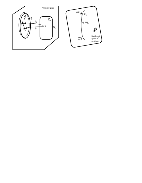
Figure 1: The boundary $S$ of $D$ is represented by a thick curve and its variation by a thin curve. The variation $\delta\mathbf{\varphi}$ of the family $\{\mathbf{\varphi}_{\eta}\}$ of varied paths belongs to $T_{\mathbf{\varphi}}(\mathbf{\wp})$, tangent space of $\mathbf{\wp}$ at $\mathbf{\varphi}$.

The virtual work concept, dual of Newton’s method, can be written in the following form:
The virtual work $\delta\tau$ is a linear functional value of the virtual displacement,

$$\delta\tau=<\Im,\delta\mathbf{\varphi}>$$ (3)

where $<.\,,.>$ denotes the inner product of $\Im$ and $\delta\mathbf{\varphi}$, with $\Im$ belonging to the cotangent space $T_{\mathbf{\varphi}}^{*}(\mathbf{\wp})$ of $\mathbf{\wp}$ at $\mathbf{\varphi}$.

In Relation (3), the medium in position $\mathbf{\varphi}$ is submitted to covector $\Im$ denoting all the ”stresses” in mechanics. In the case of motion, we must add the inertial forces, corresponding to the accelerations of masses, to the volume forces.

The d’Alembert-Lagrange principle of virtual work is expressed as follows

For all virtual displacements, the virtual work is null.

The principle leads to the analytic representation

$$\forall\ \delta\mathbf{\varphi}\in\mathit{T}_{\mathbf{\varphi}}(\mathbf{\wp}),\ \delta\tau=0$$

Theorem:   If expression (3) is a distribution expressed in a separated form [15], the d’Alembert-Lagrange principle yields the equation of motion and boundary conditions in the form  $\Im=0$ .

The virtual displacement is submitted to constraints coming from the constitutive equations and geometrical assumptions such as the mass conservation. Consequently, the constraints are not expressed by Lagrange multipliers but are directly taken into account by the variations of the constitutive equations. The equation of motion and boundary conditions result from the explicit expression of $\delta\tau$ associated with the considered physical problem. As a first example, the simplest case of theory of capillarity at equilibrium is considered.

2.2 The classical Laplace theory of capillarity

Liquid-vapor and two-phase interfaces are represented by material surfaces endowed with an energy related to the Laplace free energy of capillarity. When working far from critical conditions, the capillary layer has a thickness equivalent to a few molecular beams [16, 17] and the interface appears as a geometrical surface separating two media, with its own characteristic behavior and energy properties [18]. The domain $D$ of a compressible fluid (liquid) is immersed in a three Euclidian space. The boundary of the domain $D$ is a surface $S$ shared in $N$ parts $S_{p}$ of class $C^{2}$, $(p=1,...,N)$ (Fig. 2). We denote by $(R_{m})^{-1}$ the mean curvature of $S$; the union of the limit edges $\Gamma_{pq}$ between surfaces $S_{p}$ and $S_{q}$ is assumed to be of class $C^{2}$ and $\mathbf{t}_{p}$ is the tangent vector to $\Gamma_{p}=\bigcup\,\Gamma_{pq},q=1,...,N\ {\mathrm{w}ith}\ q\neq p$, oriented by the unit external vector to $D$ denoted $\mathbf{n}_{p}$; $\mathbf{n}_{p}^{\prime}=\mathbf{t}_{p}\times\mathbf{n}_{p}$ is the unit external normal vector to $\Gamma_{p}$ in the tangent plane to $S_{p}$; the edge $\Gamma$ of $S$ is the union of the edges $\Gamma_{p}$ of $S_{p}$.

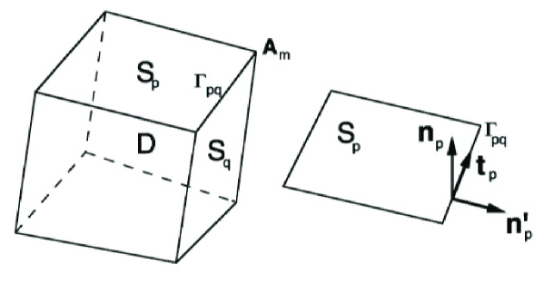
Figure 2: The set $D$ has a surface boundary $S$ divided in several parts. The edge of $S$ is denoted by $\Gamma$ which is also divided into several parts with end points $\mathbf{A}_{m}$.

To first verify the well-founded of the model, we consider the explicit expression of the functional $\delta\tau$ for compressible fluids with capillarity in non-dissipative case. The variation of the total energy $E$ of such a fluid results from the variation of the sum of the local density of energy integrated on the domain $D$ and the variation of the local density of surface energy integrated on its boundary $S$; to these variations, we must add the work of volume force $\rho\,\textbf{f}$ in $D$, surface force $\mathbf{T}$ on $S$ and line force $\mathbf{L}$ on $\Gamma$. Such an amount represents, for the domain $D$, the virtual work of forces of the compressible fluid with capillarity.
The Laplace theory of capillarity introduces the notion of surface energy (or superficial energy) on surfaces such that, for a compressible liquid with capillary effects on the wall boundaries, the total energy of the fluid writes in the form

$$E=\int\int\int_{D}\rho\ \alpha(\rho)\ dv+\int\int_{S}\sigma\ ds,\quad\mathrm{with}\quad\int\int_{S}\sigma\ ds\equiv\sum_{p=1}^{N}\int\int_{S_{p}}\sigma_{p}\ ds,$$

where $\rho$ is the matter density, $\alpha(\rho)$ is the fluid specific energy ($\rho\,\alpha(\rho)$ is the volume energy) and the coefficients $\sigma_{p}$ are the surface energy densities on each surface $S_{p}$ represented -for the sake of simplicity- by $\sigma$ on $S$ (). Surface integrations are associated with the metric space. As proved in Appendix, the variation of the deformation gradient tensor $F=\partial\mathbf{x}/\partial\mathbf{X}$ (with components $\{\partial x_{i}/\partial X_{j}\}$) of the mapping $\mathbf{\varphi}$ combined with the mass conservation and the variation of $\sigma$ allow to obtain the variation $-\delta E$ (see Eq. (27) in Appendix); then the independent variables come from the position $\mathbf{x}$ of the continuous medium.
The virtual work of volume forces defined on $D$ is generally in the form

$$\int\int\int_{D}\rho\ \mathbf{f}^{T}\mathbf{\zeta}~{}dv,\quad\mathrm{with}\quad\mathbf{f}=-\mathop{\mathrm{g}rad}\ U$$

where $U(\mathbf{x})$ is a potential per unit mass and superscript ^T denotes the transposition. The virtual work of surface and line forces defined on $S$ and $\Gamma$ are respectively,

$$\int\int_{S}\ \mathbf{T}^{T}\mathbf{\zeta}~{}ds\quad\mathrm{and}\quad\int_{\Gamma}\ \mathbf{L}^{T}\mathbf{\zeta}~{}dl.$$

Consequently, the total virtual work of forces $\delta\tau$ is

$$\delta\tau=-\delta E+\int\int\int_{D}\rho\ \mathbf{f}^{T}\mathbf{\zeta}~{}dv+\int\int_{S}\ \mathbf{T}^{T}\mathbf{\zeta}~{}ds+\int_{\Gamma}\ \mathbf{L}^{T}\mathbf{\zeta}~{}dl.$$

From Eqs. (27) and (30) in Appendix, we obtain

$$\delta\tau \equiv \int\int\int_{D}\left(-\mathrm{{grad}^{T}}p+\rho\,\mathbf{f}^{T}\right)\mathbf{\zeta}~{}dv\ +\int_{\Gamma}\left(\mathbf{L}^{T}-\sigma\,\mathbf{n}^{\prime T}\right)\mathbf{\zeta}~{}dl\$$

$$+\int\int_{S}\left[-\delta\sigma+\left\{\left({p}\,+\frac{2\,\sigma}{R_{m}}\right)\,\mathbf{n}^{T}+\mathrm{grad}^{T}\sigma\left(\mathbf{1}-\mathbf{nn}^{T}\right)+\mathbf{T}^{T}\right\}\mathbf{\zeta}\right]~{}ds$$

where $p\equiv\rho^{2}\alpha^{\prime}(\rho)$ is the pressure of the liquid [19], $\delta\sigma$ denotes the variation of the surface energy $\sigma$ and 1 denotes the identity tensor. When $\sigma$ is constant we get $\delta\sigma=0$; then,

$$\delta\tau \equiv \int\int\int_{D}\left(-\mathrm{{grad}^{T}}p+\rho\,\mathbf{f}^{T}\right)\mathbf{\zeta}~{}dv\ +\int\int_{S}\left\{\left(p+\frac{2\,\sigma}{R_{m}}\right)\,\mathbf{n}^{T}+\mathbf{T}^{T}\right\}\mathbf{\zeta}~{}ds$$

$$+\int_{\Gamma}\left(\mathbf{L}^{T}-\sigma\,\mathbf{n}^{\prime T}\right)\mathbf{\zeta}~{}dl.$$

and the d’Alembert-Lagrange principle yields the equation of equilibrium on $D$,

$$-p_{,i}+\rho f_{i}=0\quad\mathrm{or}\quad-\mathrm{grad}\,p+\rho\,\mathbf{f}=0.$$ (5)

The condition on boundary surface $S$ is,

$$\left(p+\dfrac{2\,\sigma}{R_{m}}\right)\,n_{i}+T_{i}=0\quad\ \mathrm{or}\quad\ \left(p\,+\dfrac{2\,\sigma}{R_{m}}\,\right)\mathbf{n}+\mathbf{T}=0\ ,$$ (6)

where, for an external fluid bordering $D$, $\mathbf{T}=-P\,\mathbf{n}$, with $P$ value of the pressure in the external fluid. On the lines, it is necessary to consider the partition of $S$ such that the edge $\Gamma_{pq}$ is common to $S_{p}$ and $S_{q}$,

$$\sigma_{p}\,n_{pi}^{\prime}+\sigma_{q}\,n_{qi}^{\prime}-L_{i}=0\qquad\ \mathrm{or}\qquad\ \sigma_{p}\,\mathbf{n}_{p}^{\prime}+\sigma_{q}\,\mathbf{n}_{q}^{\prime}-\mathbf{L}=0.$$ (7)

Surface condition (6) is the Laplace equation and line condition (7) is the Young-Dupré equation with a line tension L.
It is interesting to note that in [20], Steigmann and Li used the principle of virtual work by utilizing a system of line coordinates on boundary surfaces and lines. By introducing the free energy per unit area of interfaces and the free energy per unit of contact curve, they obtained Laplace’s equation and a generalization of Young-Dupré’s equation of equilibrium; moreover, by employing necessary conditions for energy-minimizing states of fluid systems they got a demonstration that the line tension associated with a three-phase contact curve must be nonnegative.

When $\sigma$ is not constant but $\delta\sigma=0$, we obtain the same equations for Eq. (5) and Eq. (7) but Eq. (6) on $S$ is replaced by

$$\left(p\,+\dfrac{2\,\sigma}{R_{m}}\right)\mathbf{n}+\left(\mathbf{1}-\mathbf{nn}^{T}\right)\mathrm{grad}\,\sigma+\mathbf{T}=0.$$

The additive term $\left(\mathbf{1}-\mathbf{nn}^{T}\right)\mathrm{grad}\,\sigma=\mathrm{grad}_{tg}\sigma$ is the tangential part of $\mathrm{grad}\,\sigma$ to the surface $S$. This term corresponds to a shear stress necessarily balanced by the tangential component of $\mathbf{T}$. Such is the case when $\sigma$ is defined on $S_{0}$ image of $S$ in the reference space $D_{0}$ (then, $\sigma=\sigma_{0}(\mathbf{X})$). We understand the importance of the surface energy constitutive behavior; this questioning is emphasized in the following section.

3 Capillarity of liquid in contact with solid and gas in presence of non-constant surface energy

We have seen in the previous section that the problem associated with the behavior of the surface energy is the key point to obtain the boundary conditions on interfaces and contact lines bordering the fluid bulk. In this section we consider a very special case of surfactant: the interfaces are endowed with a concentration of matter which affects the surface energy. The surface matter is attached to the particles of the fluid such that they obey together to the same Eq. (1) of motions and Eq. (2) of virtual motions. We consider a more general case than in Section 2.2: we study the motion of the continuous medium with viscous forces. This viscosity affects not only the equation of motion but also the boundary conditions.

3.1 Geometrical description of the continuous medium

A drop of liquid fills the set $D$ and lies on the surface of a solid. The liquid drop is also bordered by a gas. All the interfaces between liquid, solid and gas are assumed to be regular surfaces.

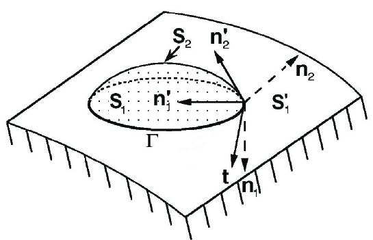
Figure 3: A liquid in drop form lies on a solid surface. The liquid is bordered with a gas and a solid; $S{{}_{1}}$ is the boundary between liquid and solid; $S^{\prime}_{1}$ is the boundary between gas and solid; $S_{2}$ is the interface between liquid and gas ; $\mathbf{n}_{1}$ and $\mathbf{n}_{2}$ are the unit normal vectors to $S_{1}$ and $S_{2}$, external to the domain of liquid; the edge $\Gamma$ (or contact line) is common to $S_{1}$ and $S_{2}$ and $\mathbf{t}$ is the unit tangent vector to $\Gamma$ relative to $\mathbf{n}_{1}$; $\mathbf{n^{\prime}}_{1}=\mathbf{n}_{1}\times\mathbf{t}$ and $\mathbf{n^{\prime}}_{2}=\mathbf{n}_{2}\times(-\mathbf{t})$ are the binormals to $\Gamma$ relative to $S_{1}$ and $S_{2}$, respectively.

We call $\sigma_{{}_{S_{1}}}$ and $\sigma_{{}_{S_{2}}}$ the values of the surface energies of $S_{1}$ and $S_{2}$, respectively (see Fig. 3). These energies may depend on each point of the boundary of $D$. Afterwards, on the domain $S_{1}^{\prime}$, the surface energy between gas and solid is neglected [21]. The liquid drop is submitted to a volume force $\rho\,\mathbf{f}$. The $\mathit{external}$ surface force on $D$ is modelized with two constraint vector fields $\mathbf{T}_{1}$ on the solid surface, $S_{1}$ and $\mathbf{T}_{2}$ on the free surface, $S_{2}$. The line tension $\mathbf{L}$ is assumed to be null.
By using the principle of virtual work, we aim to write the motion equation of the liquid drop and the conditions on surfaces and line bordering the liquid drop.

3.2 Surfactant attached to interfacial fluid particles

To express the behavior of the surface energy, we need to represent first the equation of the surface matter density.
By using the mapping $\mathbf{\varphi}$, the set $D_{0}$ of boundary $S_{0}$ has the image $D$ of boundary $S$. We assume there exists an insoluble surfactant with a surface mass concentration $c_{0}$ defined on $D_{0}$ of image $c$ in $D$ [18, 21, 22]. Let us consider the case when the surfactant is attached to the fluid particles on the surface $S$, i.e.

$$c_{0}=c_{0}(\mathbf{X}),\quad\mathrm{{where}\ \mathbf{X}\in S_{0}\,.}$$ (8)

The mass conservation of the surfactant on the surface $S$ requires that for any subset $S_{0}^{\ast}$ of $S_{0}$, of image $S^{\ast}$ subset of $S$,

$$\int\int_{S^{\ast}}c\ ds=\int\int_{S_{0}^{\ast}}c_{0}\ ds_{0}.$$ (9)

Relation (9) implies

$$c\ \det F\ \mathbf{n}_{0}^{T}F^{-1}\mathbf{n}=c_{0}\quad\mathrm{with}\quad\mathbf{n}_{0}^{T}=\frac{\mathbf{n}^{T}F}{\sqrt{(\mathbf{n}^{T}FF^{T}\mathbf{n})}}\,,$$ (10)

where $\mathbf{n}_{0}$ denotes the unit normal vector to $S_{0}$. The proof of Rel. (10) is given in Appendix.
From Rel. (8) and Rel. (10), we obtain:
Firstly, the conservation of the surface concentration of the surfactant,

$$\frac{dc}{dt}+c\left(\mathop{\mathrm{d}iv}\mathbf{u}-\mathbf{n}^{T}\mathbf{D}\ \mathbf{n}\right)=0,$$ (11)

where $\mathbf{u}$ is the fluid velocity vector and $\mathbf{D}=\frac{1}{2}\left({\partial\mathbf{u}}/{\partial\mathbf{x}}+\left({\partial\mathbf{u}}/{\partial\mathbf{x}}\right)^{T}\right)$ denotes the rate of the deformation tensor of the fluid. The term  $\mathop{\mathrm{d}iv}\mathbf{u}-\mathbf{n}^{T}\mathbf{D}\ \mathbf{n}$  expresses the tangential divergence relative to the surface $S$.
Secondly, the variation of the mass concentration of the surfactant,

$$\delta c+c\left[\mathop{\mathrm{d}iv}\mathbf{\zeta}-\mathbf{n}^{T}\frac{\partial\mathbf{\zeta}}{\partial\mathbf{x}}\,\mathbf{n}\right]=0.$$ (12)

The proofs of Relations (11) and (12) are also given in Appendix. In the case when the surface energy $\sigma$ is a function of the surfactant concentration,

$$\sigma=\sigma(c),$$

we deduce $\delta\sigma=\sigma^{\prime}(c)\,\delta c$. If we denote

$$\gamma=\sigma-c\ \sigma^{\prime}(c)\,,$$ (13)

which is the Legendre transformation of $\sigma$ with respect to $c$, then by taking Rel. (27) into account, we obtain in Appendix,

$$\delta E=-\int\int_{S}\left[\,\frac{2\gamma}{R_{m}}\,\mathbf{n}^{T}+\mathrm{{grad}^{T}\gamma\ \left(\mathbf{1}-\mathbf{nn}^{T}\right)}\right]\mathbf{\zeta}~{}ds+\int_{\Gamma}\gamma\ \mathbf{n}^{\prime T}\mathbf{\zeta}~{}dl.$$ (14)

As we shall see in Section 4, $\gamma$ is the surface tension of the interface $S$. The variation $\delta c$ of the concentration has an important consequence on the surfactant behavior and the surfactant behavior is essential to determine the virtual work of the liquid drop.
Relation (13) can easily be extended to several surfactants: if $\sigma=\sigma(c_{1},\ldots,c_{n})$ where $\displaystyle c_{i},\ i\in\{1,\ldots,n\}$ are the concentrations of $n$ surfactants, then

$$\gamma=\sigma-\sum_{i=1}^{n}c_{i}\,\frac{\partial\sigma}{\partial c_{i}}\ ,$$

corresponding to the Legendre transformation of $\sigma$ with respect to $c_{i},\ i\in\{1,\ldots,n\}$ and Eq. (14) is always valid.

3.3 Governing equation of motion and boundary conditions

As previously indicated, we do not consider the thermodynamical problem of interfaces, but for example, when the medium is isothermal, $\alpha$ can be considered as the specific free energy of the bulk and $\sigma$ the free surface energy of the interface.
The use of virtual displacements yields a linear functional of virtual work, sum of several partial works. To enumerate the works of forces, we have to consider how they are obtained in the literature [2, 3, 5]. The virtual work expressions of volume force $\rho\,\mathbf{f}$, surface force $\mathbf{T}$ and liquid pressure $p$ are the same as in Section 2.2.

a) For fluid motions, the virtual work of mass impulsions is

$$-\int\int\int_{D}\rho\ \mathbf{a}^{T}\mathbf{\zeta}~{}dv,$$

where $\mathbf{a}$ is the acceleration vector.
b) For dissipative motions, we must add the virtual work of viscous stresses

$$-\int\int\int_{D}\mathtt{tr}\left(\mathbf{\tau}_{v}\frac{\partial\mathbf{\zeta}}{\partial\mathbf{x}}\right)~{}dv,$$

where $\mathbf{\tau}_{v}$ denotes the viscous stress tensor usually written in the form of Navier-Stokes [21]. Taking account of the relation

$$\mathtt{tr}\left(\mathbf{\tau}_{v}\,\frac{\partial\mathbf{\zeta}}{\partial\mathbf{x}}\right)=\mathop{\mathrm{d}iv}(\mathbf{\tau}_{v}\,\mathbf{\zeta})-({\mathop{\mathrm{d}iv}}\mathbf{\tau}_{v})\,\mathbf{\zeta},$$

an integration by parts using Stokes’ formula in Eq. (14) for the virtual work of interfacial forces, and relations $\mathbf{n^{\prime}}_{1}=\mathbf{n}_{1}\times\mathbf{t}$, $\mathbf{n^{\prime}}_{2}=-\mathbf{n}_{2}\times\mathbf{t}$, allow to obtain the virtual work of forces applied to the domain $D$

$$\begin{array}[]{l}\delta\tau=\displaystyle\int\int\int_{D}\left(-\,{\mathop{\mathrm{g}rad}}^{T}p+\mathop{\mathrm{d}iv}\mathbf{\tau}_{v}+\rho\,\mathbf{f}^{T}-\rho\ \mathbf{a}^{T}\right)\mathbf{\zeta}~{}dv\\ \ +\displaystyle\int\int_{S_{1}}\left[{{\mathop{\mathrm{g}rad}}^{T}\gamma_{1}\left(\mathbf{1}-\mathbf{n}_{1}\mathbf{n}_{1}^{T}\right)+\left(p+{\frac{2\gamma_{1}}{R_{m_{1}}}}\right)\,\mathbf{n}_{1}^{T}}-{\mathbf{n}_{1}^{T}}\mathbf{\tau}_{v}+\mathbf{T}_{1}^{T}\right]\mathbf{\zeta}~{}ds\\ +\displaystyle\int\int_{S_{2}}\left[{{\mathop{\mathrm{g}rad}}^{T}\gamma_{2}\left(\mathbf{1}-\mathbf{n}_{2}\mathbf{n}_{2}^{T}\right)+\left(p+{\frac{2\gamma_{2}}{R_{m_{2}}}}\right)\,\mathbf{n}_{2}^{T}}-{\mathbf{n}_{2}^{T}}\mathbf{\tau}_{v}+\mathbf{T}_{2}^{T}\right]\mathbf{\zeta}~{}ds\\ \quad\displaystyle+\int_{\Gamma}\left(\,\gamma_{1}\mathbf{n}_{1}^{{}^{\prime}T}-\gamma_{2}\mathbf{n}_{2}^{{}^{\prime}T}\right)\mathbf{\zeta}~{}dl,\end{array}$$ (15)

where $R_{m_{i}}$ denotes the mean radius of curvature of $S_{i}$, $\gamma_{i}$ denotes the surface tension of $S_{i}$ and $\mathbf{T}_{i}$ the surface force on $S_{i}$, $i\in\{1,2\}$; $\mathbf{T}_{2}=-\,P\mathbf{n}_{2}$, where $P$ is the pressure in the external gas to the domain $D$.
The field of virtual displacement $\mathbf{x\in\ }D\longrightarrow\mathbf{\zeta(x)\in\ }T_{\mathbf{x}}(D)$ must be tangent to the solid (rigid) surface $S_{1}$. The fundamental lemma of variational calculus yields the equation of motion associated to domain $D$, the conditions on surfaces $S_{1}$, $S_{2}$ and the condition on contact line $\Gamma$.
Due to the fact that Eq. (15) is expressed in separate form in the sense of distributions [15], the d’Alembert-Lagrange principle implies that $\forall\ \mathbf{\zeta(x)\in\ }T_{\mathbf{x}}(D)$ tangent to $S_{1}$, each of the four integrals of Eq. (15) is null. Then, we obtain equations on $D$, $S_{1}$, $S_{2}$ and $\Gamma$, respectively.

$\bullet\quad$ We get the equation of motion in $D$

$$\rho\ \mathbf{a}+\mathop{\mathrm{g}rad}p=\left(\mathop{\mathrm{d}iv}\mathbf{\tau}_{v}\right)^{T}+\rho\,\mathbf{f}.$$ (16)

Equation (16) is the Navier-Stokes equation for compressible fluids when $\mathbf{\tau}_{v}$ is written in the classical linear form by using the rate of the fluid deformation tensor, $\mathbf{\tau}_{v}=\lambda(\mathrm{{tr}\,\mathbf{D)}\,\mathbf{1}+2\mu\,\mathbf{D}}$. We may add a classical condition for the velocity on the boundary as the adherence condition.

$\bullet\quad$ We get the condition on surface $S_{1}$

The virtual displacement is tangent to $S_{1}$; the constraint $\mathbf{n}_{1}^{T}\mathbf{\zeta}=0$ implies there exists a scalar Lagrange multiplier $\mathbf{x\in}$ $S_{1}\longrightarrow\chi\left(\mathbf{x}\right)\in\Re$, such that

$$\left(p\,+\frac{2\gamma_{1}}{R_{m_{1}}}\,\right)\mathbf{n}_{1}-\mathbf{\tau}_{v}\mathbf{n}_{1}+\left(\mathbf{1}-\mathbf{n}_{1}\mathbf{n}_{1}^{T}\right)\mathop{\mathrm{g}rad}\gamma_{1}+\mathbf{T}_{1}=\chi\,\mathbf{n}_{1},$$ (17)

The normal and tangential components of Eq. (17) relative to $S_{1}$ are deduced from Eq. (17),

$$\displaystyle\ p+\frac{2\gamma_{1}}{R_{m_{1}}}-\mathbf{n}_{1}^{T}\mathbf{\tau}_{v}\,\mathbf{n}_{1}+\mathbf{n}_{1}^{T}\,\mathbf{T}_{1}=\chi,$$ (18)

$$\left(\mathbf{1}-\mathbf{n}_{1}\mathbf{n}_{1}^{T}\right)\left(-\mathbf{\tau}_{v}\mathbf{n}_{1}+\mathop{\mathrm{g}rad}\gamma_{1}+\mathbf{T}_{1}\right)=0\,.$$ (19)

Following Eq. (18), we obtain the value of $\chi$ along the surface $S_{1}$. The scalar field $\chi$ corresponds to the unknown value of the normal stress vector on the surface $S_{1}$; it corresponds to the difference between the mechanical and viscous normal stresses and a stress due to the curvature of $S_{1}$ taking account of the surface tension. Equation (19) represents the balance between the tangential components of the mechanical and viscous stresses and the tangential component of the surface tension gradient.

$\bullet\quad$ We get the condition on surface $S_{2}$

$$\left(p\,+\frac{2\gamma_{2}}{R_{m_{2}}}\,\right)\mathbf{n}_{2}-\mathbf{\tau}_{v}\mathbf{n}_{2}+\left(\mathbf{1}-\mathbf{n}_{2}\mathbf{n}_{2}^{T}\right)\mathop{\mathrm{g}rad}\gamma_{2}-P\,\mathbf{n}_{2}=0.$$ (20)

The normal and tangential components of Eq. (20) relative to $S_{2}$ are deduced

$$\frac{2\gamma_{2}}{R_{m_{2}}}-\mathbf{n}_{2}^{T}\mathbf{\tau}_{v}\,\mathbf{n}_{2}+p=P,$$ (21)

$$\left(\mathbf{1}-\mathbf{n}_{2}\mathbf{n}_{2}^{T}\right)\left(-\mathbf{\tau}_{v}\mathbf{n}_{2}+\mathop{\mathrm{g}rad}\gamma_{2}\right)=0.$$ (22)

Equation (21) corresponds to the expression of the Laplace equation in case of viscous motions; the normal component of viscous stresses is taken into account. Equation (22) is similar to Eq. (19) for the surface $S_{2}$ but without component of the stress vector.

$\bullet\quad$ We get the condition on line $\Gamma$

To get the line condition we must consider a virtual displacement tangent to $S_{1}$ and consequently in the form

$$\mathbf{\zeta}=\alpha\,\mathbf{t}+\beta\,\mathbf{t}\times\mathbf{n}_{1},$$

where $\alpha$ and $\beta$ are two scalar fields defined on $\Gamma$. From the last integral of Eq. (15), we get immediately:
For any scalar field $\mathbf{x\in}$ $\Gamma\longrightarrow\beta\left(\mathbf{x}\right)\in\Re,$

$$\int_{\Gamma}\beta\gamma_{1}\,\mathbf{n}_{1}^{\prime T}\left(\mathbf{t}\times\mathbf{n}_{1}\right)~{}dl-\int_{\Gamma}\beta\gamma_{2}\,\mathbf{n}_{2}^{\prime T}\left(\mathbf{t}\times\mathbf{n}_{1}\right)~{}dl=0,$$

with $\mathbf{n^{\prime}}_{1}=-\mathbf{t}\times\mathbf{n}_{1}$ and $\mathbf{n^{\prime}}_{2}=\mathbf{t}\times\mathbf{n}_{2}$ and consequently,

$$-\gamma_{1}-\gamma_{2}\,\mathbf{n}_{2}^{T}\mathbf{n}_{1}=0.$$

Denoting by $\theta$ the angle $<\mathbf{n}_{1},\mathbf{n}_{2}>$, we obtain the well-known relation of Young-Dupré but adapted to $\gamma_{1}$ and $\gamma_{2}$ in place of $\sigma_{1}$ and $\sigma_{2}$

$$\gamma_{1}+\gamma_{2}\cos\theta=0.$$ (23)

3.4 Remarks

For a motionless fluid, ${\mathbf{\tau}}_{v}=0$ and consequently:

Equation (19) yields,

$$\mathrm{grad}_{tg}\gamma_{1}=-\mathbf{T}_{1tg},$$

where $\mathrm{grad}_{tg}\gamma_{1}$ and $\mathbf{T}_{1tg}$ denote the tangential parts of $\mathrm{grad}\,\gamma_{1}$ and $\mathbf{T}_{1}$, respectively. The tangential part of the vector stress is opposite to the surface tension gradient. Therefore, at given value of $T_{1n}=\mathbf{n}_{1}^{T}\mathbf{T}_{1}$, Eq. (18) yields the value $\chi$ corresponding to the normal stress vector to the surface $S_{1}$,
Equation (21) yields $\displaystyle P=p+\frac{2\,\gamma_{2}}{R_{m_{2}}}$ corresponding to the classical equation of Badshforth and Adams [21] but with the surface tension $\gamma_{2}$ instead of $\sigma_{2}$,
Equation (22) implies $\left(\mathbf{1}-\mathbf{n}_{2}\mathbf{n}_{2}^{T}\right)\mathop{\mathrm{g}rad}\gamma_{2}=0$. At equilibrium, along $S_{2}$, the surface tension $\gamma_{2}$ must be uniform.

In case of motion, Eq. (22) represents the Marangoni effect as proposed in [22, 23] but with the surface tension $\gamma_{2}$ instead of $\sigma_{2}$.

4 Surface energy and surface tension

A surface tension must appear on the boundary conditions as a force per unit of line. The Legendre transformation $\gamma$ of $\sigma$ with respect to $c$ exactly corresponds to this property on the contact line $\Gamma$; then, surface tension $\gamma$ differs from the surface energy; this important property was pointed out by Gibbs [23] and Defay [22] by means of thermodynamical considerations. The fundamental difference between surface tension and surface energy, in presence of attached surfactants, is illustrated in the following cases corresponding to formal behaviors.
- If $\sigma$ is independant of $c$, then $\gamma=\sigma$ : the surface tension is equal to the surface energy. This is the classical case of capillarity for fluids considered in Section 2.2 and Eq. (23) is the classical Young-Dupré condition on the contact lines.
- In fact $\sigma$ is a decreasing function of $c$ [21]; when $c$ is small enough we consider the behavior

$$\sigma=\sigma_{0}-\sigma_{1}\,c\quad\mathrm{where}\ \sigma_{0}>0\ \mathrm{and}\,\ \sigma_{1}>0\,,$$

then, Eq. (13) implies $\gamma=\sigma_{0}$ and surface tension and surface energy are different.
- Now, we consider a formal case when the surface energy density model writes in the form

$$\sigma=\sigma_{0}-\sigma_{1}\,c-\sigma_{2}\,c\,\sin\left(\frac{1}{c}\right)$$

where $\sigma_{0}>0,\,\sigma_{1}>0,\,\sigma_{2}>0$. Then, Eq. (13) implies

$$\gamma=\sigma_{0}-\sigma_{2}\cos\left(\frac{1}{c}\right).$$ (24)

This case does not correspond to $\sigma$ as a monotonic decreasing function of $c$. Nevertheless, when $c$ $\rightarrow 0$, $\gamma$ does not have any limit and we get

$$\gamma\in\left[\sigma_{0}-\sigma_{2},\sigma_{0}+\sigma_{2}\right].$$

The surface tension may have a large scale of values. When the concentration $c$ is low, a variation of the concentration $c$ may generate strong fluctuations of the surface tension without significant change of the surface energy. Alternatively, the concentration behavior strongly affects the surface tension but not the surface energy. Relation (24) fits with the well-known physical case of an hysteresis behavior for a drop lying on a horizontal plane (see for example [24] and the literature therein). So, the surface roughness is not the only reason of the hysteresis of the contact angle even if the surface energy is nearly constant.

5 Conclusion

The principle of virtual work allows us to deduce the equation of motion and conditions on surfaces and line by means of a variational analysis. When capillary forces operate and surfactant molecules are attached to the fluid molecules at the interfaces, the conditions on surfaces and lines point out a fundamental difference between the concepts of surface energy and surface tension. This fact was thermodynamically predicted in [22, 23]. Hysteresis phenomenon may appear even if surface energy is almost constant on a planar substrate when the surface tension strongly varies.
In Eq. (23), $\gamma_{1}$ and $\gamma_{2}$ are not assumed to be constant, but are defined at each point of $\Gamma$. This expression of Young-Dupré boundary condition on the contact line $\Gamma$ is not true in more complex cases. For example in the case when the surface tension is a non-local functional of surfactant concentration, the surface tension is no longer the classical Legendre transformation of the surface energy relative to surfactant concentration and more complex behaviors can be foreseen. These behaviors can change the variation of the integral of the free energy as in the case of shells or in second gradient models for which boundary conditions become more complex [3, 25, 26, 27, 28]. In a further article [29], we will see this is also the case when the surface energy depends on the surface curvature as in membranes and vesicles [30, 31, 32].

6 Appendix - Geometrical preliminaries [33, 34, 35]

6.1 Expression of the virtual work of forces in capillarity

The hypotheses and notations are presented in the previous Section 2.2.

6.1.1 Lemma 1: we have the following relations,

$$\delta\det F = \ \det F\,\mathop{\mathrm{d}iv}\mathbf{\zeta}\,,$$ (25)

$$\delta\left(F^{-1}\mathbf{n}\right) = -F^{-1}\ \frac{\partial\mathbf{\zeta}}{\partial\mathbf{x}}\,\mathbf{n\ +\ }F^{-1}\,\delta\mathbf{n}\,.$$ (26)

The proof of Rel. (25) comes from the so-called Jacobi identity

$$\delta(\det F)=\det F\,\mathtt{tr}\left(F^{-1}\delta F\right)$$

and from

$$\delta F=\delta\left(\frac{\partial\mathbf{x}}{\partial\mathbf{X}}\right)=\frac{\partial\mathbf{\zeta}}{\partial\mathbf{X}}.$$

Then,

$$\mathtt{tr}\left(F^{-1}\delta F\right)=\mathtt{tr}\left(\frac{\partial\mathbf{X}}{\partial\mathbf{x}}\,\frac{\partial\mathbf{\zeta}}{\partial\mathbf{X}}\right)=\mathtt{tr}\left(\frac{\partial\mathbf{\zeta}}{\partial\mathbf{X}}\,\frac{\partial\mathbf{X}}{\partial\mathbf{x}}\right)=\mathtt{tr}\left(\frac{\partial\mathbf{\zeta}}{\partial\mathbf{x}}\right)=\mathrm{div}\,{\mathbf{\zeta}}.$$

The proof of Rel. (26) comes as follow

$$\delta\left(F^{-1}\mathbf{n}\right)=\delta\left(F^{-1}\right)\mathbf{n}+F^{-1}\delta\mathbf{n}$$

But the implication,

$$F^{-1}\,F=\mathbf{1}\ \Longrightarrow\ \delta\left(F^{-1}\right)F+F^{-1}\,\delta F=0\ \Longrightarrow\ \delta\left(F^{-1}\right)=-F^{-1}\frac{\partial\mathbf{\zeta}}{\partial\mathbf{X}}F^{-1}=-F^{-1}\frac{\partial\mathbf{\zeta}}{\partial\mathbf{x}},$$

yields Rel. (26).

6.1.2 Lemma 2 : Let us consider the surface integral $\ \displaystyle E=\int\int_{S}\sigma\,ds.$ Then the variation of $E$ is,

$$\delta E=\int\int_{S}\left[\delta\sigma-\left(\frac{2\sigma}{R_{m}}\,\mathbf{n}^{T}+\mathrm{{grad}^{T}\sigma\left(\mathbf{1}-\mathbf{nn}^{T}\right)}\right)\mathbf{\zeta}\right]~{}ds+\int_{\Gamma}\sigma\,\mathbf{n}^{\prime T}\mathbf{\zeta}~{}dl.$$ (27)

Relation (27) points out the extreme importance to know the variation of $\delta\sigma$. The variation $\delta E$ of $E$ drastically changes following the different possible behaviors of the surface energy.

The proof can be found as follows: the external normal ${\mathbf{n(x)}}$ to $S$ is locally extended in the vicinity of $S$ by the relation ${\mathbf{n(x)}}=\mathrm{grad}\ d(\mathbf{x}),$ where $d$ is the distance of point $\mathbf{x}$ to $S$; for any vector field ${\mathbf{w}}$, we obtain [34, 35]

$$\mathrm{rot}({\mathbf{n}}\times{\mathbf{w}})={\mathbf{n}}\,\mathrm{div}\,{\mathbf{w}}-{\mathbf{w}}\,\mathrm{div}\,{\mathbf{n}}+\frac{\partial{\mathbf{n}}}{\partial{\mathbf{x}}}\,{\mathbf{w}}-\frac{\partial{\mathbf{w}}}{\partial{\mathbf{x}}}\,{\mathbf{n}}.$$

From $\,\displaystyle{\mathbf{n}}^{T}\frac{\partial{\mathbf{n}}}{\partial{\mathbf{x}}}=0\,$ and $\,\mathrm{div}\,{\mathbf{n}}=\displaystyle-\frac{2}{R_{m}}$ , we deduce on $S$,

$${\mathbf{n}^{T}}\mathrm{rot}({\mathbf{n}}\times{\mathbf{w}})=\mathrm{div}\,{\mathbf{w}}+\frac{2}{R_{m}}\,{\mathbf{n}^{T}}{\mathbf{w}}-{\mathbf{n}^{T}}\frac{\partial{\mathbf{w}}}{\partial{\mathbf{x}}}\,{\mathbf{n}}.$$ (28)

Due to $\displaystyle\ E=\int\int_{S}\sigma\ \det\,({\mathbf{n}},d_{1}{\mathbf{x}},d_{2}{\mathbf{x}})\$ where $\displaystyle\ d_{1}{\mathbf{x}}\$ and $\displaystyle\ d_{2}{\mathbf{x}}\$ are differentiable vectors associated with two coordinate lines of $S,$ we get

$$E=\int\int_{S_{0}}\sigma\,\det\,F\ \hbox{det}\,(F^{-1}{\mathbf{n}},d_{1}{\mathbf{X}},d_{2}{\mathbf{X}}),$$

where $d_{1}{\mathbf{x}}=F\,d_{1}{\mathbf{X}}$ and $d_{2}{\mathbf{x}}=F\,d_{2}{\mathbf{X}}$. Then,

$$\delta E=\int\int_{S_{0}}\delta\sigma\ \det\,F\ \hbox{det}\,(F^{-1}{\mathbf{n}},d_{1}{\mathbf{X}},d_{2}{\mathbf{X}})+\int\int_{S_{0}}\sigma\,\delta\left(\det\,F\ \hbox{det}\,(F^{-1}{\mathbf{n}},d_{1}{\mathbf{X}},d_{2}{\mathbf{X}})\right).$$

Due to Lemma 1 and to $\,\displaystyle{\mathbf{n}}^{T}\mathbf{n}=1\,\Longrightarrow\,{\mathbf{n}}^{T}\delta\mathbf{n}=0$,

$$\begin{array}[]{cc}\displaystyle\int\int_{S_{0}}\sigma\,\delta\left(\det\,F\ \hbox{det}\,(F^{-1}{\mathbf{n}},d_{1}{\mathbf{X}},d_{2}{\mathbf{X}})\right)=&\\ \displaystyle\int\int_{S}\left[\sigma\ \mathrm{div}\,{\mathbf{\zeta}}\ \det({\mathbf{n}},d_{1}{\mathbf{x}},d_{2}{\mathbf{x}})+\sigma\,\det\left(\displaystyle\delta{\mathbf{n}},d_{1}{\mathbf{x}},d_{2}{\mathbf{x}}\right)\displaystyle-\sigma\det\left(\displaystyle\frac{\partial{\mathbf{\zeta}}}{\partial{\mathbf{x}}}\,{\mathbf{n}},d_{1}{\mathbf{x}},d_{2}{\mathbf{x}}\right)\right]=&\\ \displaystyle\int\int_{S}\left(\mathrm{div}(\sigma\,{\mathbf{\zeta}})-(\mathrm{grad}^{T}\sigma)\,{\mathbf{\zeta}}-\sigma\,{\mathbf{n}}^{T}\frac{\partial{\mathbf{\zeta}}}{\partial{\mathbf{x}}}\,{\mathbf{n}}\right)ds.&\end{array}$$

Relation (28) yields

$$\mathrm{div}\,(\sigma\,{\mathbf{\zeta}})+\frac{2\sigma}{R_{m}}\,{\mathbf{n}}^{T}{\mathbf{\zeta}}-{\mathbf{n}}^{T}\frac{\partial\sigma{\mathbf{\zeta}}}{\partial{\mathbf{x}}}\,{\mathbf{n}}={\mathbf{n}}^{T}\,\mathrm{rot}\,(\sigma\,{\mathbf{n}}\times{\mathbf{\zeta}}).$$

Then,

$$\begin{array}[]{cc}\displaystyle\int\int_{S_{0}}\sigma\,\delta\left(\det\ F\,\hbox{det}\,(F^{-1}{\mathbf{n}},d_{1}{\mathbf{X}},d_{2}{\mathbf{X}})\right)=&\\ \displaystyle\ \int\int_{S}\left(-\frac{2\sigma}{R_{m}}\,{\mathbf{n}}^{T}+\mathrm{grad}^{T}\sigma\,({\mathbf{nn}^{T}-\mathbf{1}})\right){\mathbf{\zeta}}\,ds+\int\int_{S}{\mathbf{n}}^{T}\ \mathrm{rot}\,(\sigma\,{\mathbf{n}}\times{\mathbf{\zeta}})\,ds,&\end{array}$$

where $\mathrm{grad}^{T}\sigma\,({{\mathbf{nn}}^{T}-\mathbf{1}})$ belongs to the cotangent plane to $S$ and we obtain Relation (27).

6.1.3 Variation of the internal energy

Let us note that $\displaystyle\delta\int\int\int_{D}\rho\ \alpha\,dv=\int\int\int_{D}\rho\ \delta\alpha\,dv$ where $\displaystyle\ \delta\alpha=\frac{\partial\alpha}{\partial\rho}\ \delta\rho$.
Due to the mass conservation,

$$\rho\ \mathrm{det}\,F=\rho_{0}(\mathbf{X}),$$ (29)

where $\rho_{0}$ is defined on $D_{0}$, the differentiation of Eq. (29) yields,

$$\delta\rho\,\mathrm{det}F+\rho\,\delta(\mathrm{det}F)=0$$

and from Lemma 1, we get

$$\delta\,\rho=-\rho\,\mathrm{div}\,{\mathbf{\zeta}}.$$

Consequently, from $\displaystyle p=\rho^{2}\frac{\partial\alpha}{\partial\rho}$ and $\mathrm{div}(p\,{\mathbf{\zeta}})=p\,\mathrm{div}{\mathbf{\zeta}}+(\mathrm{grad}\,p)^{T}\,{\mathbf{\zeta}}$ , we get

$$\delta\int\int\int_{D}\rho\ \alpha\,dv =$$ (30)

$$\int\int\int_{D}\rho\,\frac{\partial\alpha}{\partial\rho}\,\delta\rho\,dv = \int\int\int_{D}-p\ \mathrm{div}\,{\mathbf{\zeta}}\,dv=\int\int\int_{D}(\mathrm{grad}\,p)^{T}\,{\mathbf{\zeta}}\,dv-\int\int_{S}{p\,\mathbf{n}}^{T}{\mathbf{\zeta}}\,ds.$$

By taking account of Rel. (27), we immediately get Rel. (2.2).

6.2 Study of a surfactant attached to fluid particles

6.2.1 Proof of relation (10)

Under the hypotheses and notations of Section 3.2,

$$\int\int_{S^{\ast}}c\ ds = \int\int_{S^{\ast}}{\det}({\mathbf{n}}\,c,d_{1}{\mathbf{x}},d_{2}{\mathbf{x}})=\int\int_{S^{\ast}_{0}}{\det}({FF^{-1}\mathbf{n}}\,c,Fd_{1}{\mathbf{X}},Fd_{2}{\mathbf{X}})$$

$$= \int\int_{S_{0}^{\ast}}c\,({\det}F)\,\mathrm{det}({\ F^{-1}\mathbf{n}},d_{1}{\mathbf{X}},d_{2}{\mathbf{X}})=\int\int_{S_{0}^{\ast}}c\,(\det F)\ \mathbf{n}_{0}^{T}F^{-1}\mathbf{n}~{}ds_{0},$$

where $\mathbf{n}_{0}^{T}\,\mathbf{n}_{0}=1$. Moreover, $\mathbf{n}^{T}d{\mathbf{x}}=0\Rightarrow\mathbf{n}^{T}Fd{\mathbf{X}}=0$, then $\mathbf{n^{\prime}}_{0}^{T}=\mathbf{n}^{T}F$ is normal to $S_{0}^{\ast}$ and consequently,

$$\mathbf{n}_{0}^{T}=\frac{\mathbf{n}^{T}F}{\sqrt{(\mathbf{n}^{T}FF^{T}\mathbf{n})}}\,,\qquad\mathbf{n}^{T}=\frac{\mathbf{n}_{0}^{T}F^{-1}}{\sqrt{(\mathbf{n}^{T}_{0}F^{-1}({F^{-1}})^{T}\mathbf{n_{0}})}}$$

and from Rel. (9),

$$c\,\det F\ \sqrt{\mathbf{n}_{0}^{T}F^{-1}({F^{-1}})^{T}\mathbf{n_{0}}}=c_{0}.$$ (31)

6.2.2 Proof of relations (11) and (12)

With the notations of Section 3.2, Rel. (31) yields

$$\frac{dc}{dt}=\displaystyle-\frac{c_{0}\,\displaystyle\frac{d\,(\det F)}{dt}}{\left(\det F\right)^{2}\sqrt{\big{(}\mathbf{n}_{0}^{T}F^{-1}(F^{-1})^{T}\mathbf{n}_{0}\big{)}}}-\frac{c_{0}\,\displaystyle\frac{d}{dt}\left(\mathbf{n}_{0}^{T}F^{-1}(F^{-1})^{T}\mathbf{n}_{0}\right)}{2\det F\big{(}\mathbf{n}_{0}^{T}F^{-1}(F^{-1})^{T}\mathbf{n}_{0}\big{)}^{{3}/{2}}}.$$

But, $\displaystyle\frac{d\,(\det F)}{dt}=(\det F)\,\mathrm{div}\,\mathbf{u}$  and  $\displaystyle\frac{d}{dt}\left(F^{-1}(F^{-1})^{T}\right)=-2F^{-1}\mathbf{D}\,(F^{-1})^{T}$. Then,

$$\frac{dc}{dt}+c\left(\mathop{\mathrm{d}iv}\mathbf{u}-\mathbf{n}^{T}\mathbf{D}\ \mathbf{n}\right)=0.$$

The same calculation with $\delta$ in place of $\ \displaystyle\frac{d}{dt}\$ yields immediately

$$\delta c+c\left[\mathop{\mathrm{d}iv}\mathbf{\zeta}-\mathbf{n}^{T}\frac{\partial\mathbf{\zeta}}{\partial\mathbf{x}}\,\mathbf{n}\right]=0.$$

6.2.3 Proof of relation (14)

From Rel. (12) and $\sigma=\sigma(c)$ we get,

$$\delta\sigma=\kappa\left[\mathop{\mathrm{d}iv}\mathbf{\zeta}-\mathbf{n}^{T}\frac{\partial\mathbf{\zeta}}{\partial\mathbf{x}}\,\mathbf{n}\right]\quad{\mathrm{w}ith}\quad\kappa(c)=-c\,\sigma^{\prime}(c).$$

Consequently,

$$\int\int_{S}\delta\sigma=\int\int_{S}\left(\mathop{\mathrm{d}iv}(\kappa\,\mathbf{\zeta})-\mathrm{grad}^{T}\kappa\ \mathbf{\zeta}-\kappa\,\mathbf{n}^{T}\frac{\partial\mathbf{\zeta}}{\partial\mathbf{x}}\,\mathbf{n}\right)ds.$$

But Rel. (28) implies,

$${\mathbf{n}^{T}}\mathrm{rot}(\kappa\,{\mathbf{n}}\times{\mathbf{\zeta}})=\mathrm{div}(\kappa\,{\mathbf{\zeta}})+\frac{2\kappa}{R_{m}}\,{\mathbf{n}^{T}}{\mathbf{\zeta}}-{\mathbf{n}^{T}}\frac{\partial{(\kappa\,\mathbf{\zeta})}}{\partial{\mathbf{x}}}\,{\mathbf{n}}$$

and,

$${\mathbf{n}^{T}}\frac{\partial{(\kappa\,\mathbf{\zeta})}}{\partial{\mathbf{x}}}\,{\mathbf{n}}=(\mathbf{n}^{T}\mathbf{\zeta})\textbf{.}(\mathrm{grad}^{T}\kappa\ \mathbf{n})+\kappa\,\mathbf{n}^{T}\frac{\partial\mathbf{\zeta}}{\partial\mathbf{x}}\,\mathbf{n}=\mathrm{grad}^{T}\kappa\,\mathbf{n}\mathbf{n}^{T}\mathbf{\zeta}+\kappa\,\mathbf{n}^{T}\frac{\partial\mathbf{\zeta}}{\partial\mathbf{x}}\,\mathbf{n}.$$

Then,

$$\mathop{\mathrm{d}iv}(\kappa\,\mathbf{\zeta})-\mathrm{grad}^{T}\kappa\ \mathbf{\zeta}-\kappa\,\mathbf{n}^{T}\frac{\partial\mathbf{\zeta}}{\partial\mathbf{x}}\,\mathbf{n}=-\frac{2\kappa}{R_{m}}\,{\mathbf{n}^{T}}{\mathbf{\zeta}}-\mathrm{grad}^{T}\kappa\,(\textbf{1}-{\mathbf{n}}{\mathbf{n}^{T}})\mathbf{\zeta}+{\mathbf{n}^{T}}\mathrm{rot}(\kappa\,{\mathbf{n}}\times{\mathbf{\zeta}})$$

Due to

$$\int\int_{S}{\mathbf{n}^{T}}\mathrm{rot}(\kappa\,{\mathbf{n}}\times{\mathbf{\zeta}})\,ds=\int_{\Gamma}\kappa\,\mathbf{n}^{\prime T}\mathbf{\zeta}~{}dl,$$

we get

$$\int\int_{S}-\delta\sigma\,ds=\int\int_{S}\left[\,\frac{2\kappa}{R_{m}}\,{\mathbf{n}^{T}}+\mathrm{grad}^{T}\kappa\,(\textbf{1}-{\mathbf{n}}{\mathbf{n}^{T}})\right]\mathbf{\zeta}\,ds-\int_{\Gamma}\kappa\,\mathbf{n}^{\prime T}\mathbf{\zeta}~{}dl,$$

and Rel. (27) yields,

$$\delta E=-\int\int_{S}\left[\,\frac{2\gamma}{R_{m}}\,\mathbf{n}^{T}+\mathrm{{grad}^{T}\gamma\ \left(\mathbf{1}-\mathbf{nn}^{T}\right)}\right]\mathbf{\zeta}~{}ds+\int_{\Gamma}\gamma\ \mathbf{n}^{\prime T}\mathbf{\zeta}~{}dl.$$

References

• [1] J. Serrin, Mathematical principles of classical fluid mechanics, in Encyclopedia of Physics VIII/1, Ed: S. Flügge, pp. 125-263, Springer, Berlin, 1960.
• [2] P. Germain, La méthode des puissances virtuelles en mécanique des milieux continus, J. Mécanique 12, 235-274, 1973.
• [3] P. Germain, The method of the virtual power in continuum mechanics - Part 2 : microstructure, SIAM, J. Appl. Math., 25, 556-575, 1973.
• [4] N. Daher and G. A. Maugin, The method of virtual power in continuum mechanics: application to media presenting singular surfaces and interfaces, Acta Mechanica, 60 (3-4), 217-240, 1986.
• [5] H. Gouin, The d’Alembert-Lagrange principle for gradient theories and boundary conditions, in: Ruggeri, T., Sammartino, M. (Eds.), Asymptotic Methods in Nonlinear Wave Phenomena, World Scientific, pp. 79-95, Singapore, 2007.
• [6] P. Steinmann, On boundary potential energies in deformational and configurational mechanics, Journal of the Mechanics and Physics of Solids, 56 (3), 772-800, 2008.
• [7] R. Fosdick and H. Tang, Surface transport in continuum mechanics, Mathematics and Mechanics of Solids, 14(6), 587-598, 2009.
• [8] P. Cermelli, E. Fried and M. E. Gurtin, Transport relations for surface integrals arising in the formulation of balance laws for evolving fluid interfaces, J. Fluid Mechanics, 544, 339-351, 2005.
• [9] F. D. Fischer, T. Waitz, D. Vollath and N. K. Simha, On the role of surface energy and surface stress in phase-transforming nanoparticles, Progress in Materials Science, 53(3), 481-527, 2008.
• [10] M. J. Rosen,  Surfactants and interfacial phenomena, Wiley Interscience, New Jersey, 2004.
• [11] P. G. de Gennes, F. Brochard-Wyart and D. Quéré, Capillarity and wetting phenomena: drops, bubbles, pearls, waves, Springer, Berlin, 2004.
• [12] D. A. Edwards, H. Brenner and D. T. Wasan, Interfacial transport processes and rheology, Butterworth-Heinemann, Stoneham, 1991.
• [13] J. C. Slattery, L. Sagis and E. S. Oh, Interfacial transport phenomena, 2nd edition, Springer, 2007.
• [14] A. McBride, A. Javili, P. Steinmann and S. Bargmann, Geometrically nonlinear continuum thermomechanics with surface energies coupled to diffusion, Journal of the Mechanics and Physics of Solids, 59 (10), 2116-2133, 2011.
• [15] L. Schwartz, Théorie des distributions, Ch. 3, Hermann, Paris, 1966.
• [16] S. Ono and S. Kondo, Molecular theory of surface tension in liquid, in Encyclopedia of Physics, X, Ed: S. Flügge, p.p. 134-280, Springer, Berlin, 1960.
• [17] C. Domb, The critical point, Taylor & Francis, London, 1996.
• [18] V. Levitch, Physicochemical hydrodynamics, Prentice-Hall, New Jersey, 1962.
• [19] Y. Rocard, Thermodynamique, Masson, Paris, 1952.
• [20] D.J. Steigmann and D. Li, Energy minimizing states of capillary systems with bulk, surface and line phases, IMA J. Appl. Math. 55, 1-17, 1995.
• [21] A. W. Adamson,  Physical chemistry of surfaces, Interscience, New York, 1967.
• [22] R. Defay, Thermodynamique de la tension superficielle, Gauthier-Villars, Paris, 1971.
• [23] J. W. Gibbs, The scientific papers of J. Willard Gibbs, vol. 1, p. 234, Longmans, Green and Co, London, 1928.
• [24] H. Gouin, The wetting problem of fluids on solid surfaces. Part 2: the contact angle hysteresis, Continuum Mech. Thermodyn. 15, 597-611, 2003.
• [25] E. Cosserat and F. Cosserat, Sur la théorie des corps déformables, Hermann, Paris, 1909.
• [26] R. A. Toupin, Elastic materials with couple stresses, Arch. Rat. mech. Anal. 11, 385-414, 1962.
• [27] W. Noll and E. G. Virga, On edge interactions and surface tension, Arch. Rat. Mech. Anal. 111, 1-31, 1990.
• [28] F. dell’Isola and P. Seppecher, Edge contact forces and quasi-balanced power, Meccanica 32, 33-52, 1997.
• [29] H. Gouin, Vesicles: a capillarity model revisited (in preparation).
• [30] W. Helfrich, Elastic properties of lipid bilayers: theory and possible experiments, Z. Naturforsch. C 28, 693–703, 1973.
• [31] U. Seifert, Configurations of fluid membranes and vesicles, Adv. Phys. 46, 13–137, 1997.
• [32] A. Agrawal and D.J. Steigmann, A model for surface diffusion of trans-membrane proteins on lipid bilayers, ZAMP 62, 549-563, 2011.
• [33] H. Gouin and W. Kosiński, Boundary conditions for a capillary fluid in contact with a wall, Arch. Mech. 50, 907-916, 1998.
• [34] R. Aris, Vectors, tensors, and the basic equations of fluid mechanics, Dover Publications, 1989
• [35] S. Kobayashi, K. Nomizu, Foundations of differential geometry, vol. 1, Interscience Publ., New York, 1963.