Hybrid Monte-Carlo simulation of interacting tight-binding model of graphene

Abstract:

In this work, results are presented of Hybrid-Monte-Carlo simulations of the tight-binding Hamiltonian of graphene, coupled to an instantaneous long-range two-body potential which is modeled by a Hubbard-Stratonovich auxiliary field. We present an investigation of the spontaneous breaking of the sublattice symmetry, which corresponds to a phase transition from a conducting to an insulating phase and which occurs when the effective fine-structure constant $\alpha$ of the system crosses above a certain threshold $\alpha_{C}$. Qualitative comparisons to earlier works on the subject (which used larger system sizes and higher statistics) are made and it is established that $\alpha_{C}$ is of a plausible magnitude in our simulations. Also, we discuss differences between simulations using compact and non-compact variants of the Hubbard field and present a quantitative comparison of distinct discretization schemes of the Euclidean time-like dimension in the Fermion operator.

1 Introduction

In recent years, much interest has arisen in the properties of graphene, a one atom thick sheet of carbon atoms arranged on a hexagonal ”honeycomb” lattice. It has become clear that such a simple structure generates a magnitude of unusual quantum effects, which not only make graphene a promising candidate for a wide range of technological applications but also a great model system to study processes commonly associated with high-energy physics. The later stems from the fact that the tight-binding Hamiltonian which describes electrons in the $\pi$-orbitals of the carbon atoms (with additional terms describing electromagnetic two-body interactions) is well approximated by a variant of Quantum Electrodynamics in $2+1$ dimensions in the limit of low energies (see e.g. Ref. [2]). In this limit, electronic quasi-particles behave as massless Dirac particles, with a relativistic dispersion relation. In contrast to QED however the interacting theory is strongly coupled, since the small Fermi velocity of $v_{F}\approx c/300$ of the electrons generates an effective fine structure constant which is $\alpha\approx 300/137\approx 2.2$.

It is this surprising connection to relativistic field-theory which drove the high-energy physics community to take interest in graphene. The strongly coupled nature of the interacting system motivated the utilization of established non-perturbative methods such as the simulation in discretized spacetimes. One of the main questions in such studies, which is of direct consequence to technological applications, is whether or not there exists a band-gap in the interacting system which is absent in a pure tight-binding model. This corresponds to a spontaneous breaking of the symmetry under exchange of the two triangular sublattices of the graphene sheet and is mapped onto chiral-symmetry breaking in the low-energy effective theory. Moreover, graphene allows for a tuning of the effective coupling constant, by affixing the sheet to a substrate which generates dielectric screening. It is thus of interest whether a phase-transition from a conducting to an insulating phase takes place for some value of $\alpha$, and whether the critical value lies in a range which can be experimentally realized (suspended graphene giving an upper bound). Since recent experiments provide evidence that graphene in vacuum is in fact a conductor [3], it is important to establish model calculations which match the observation.

Early attempts at simulating graphene on the lattice studied the low-energy limit only, since the application of QCD methods is most direct here. Most prominently, Refs. [4] simulated the low-energy theory using staggered Fermions, whereas Ref. [5] investigated a variant of the Thirring model which has many similarities with $\textrm{QED}_{2+1}$. Both find a phase transition to a gapped phase for $\alpha>\alpha_{C}\approx 1$, which is well within the physical region. More recently, a path integral formulation of the partition function was derived directly from the tight-binding theory, which preserves the hexagonal structure of graphene and employs unphysical discretization in the time dimension only [6], with the spatial lattice spacing as a free parameter that can be taken from experiment. In this formulation, interactions are modeled by a non-local potential which is generated by a Hubbard-Stratonovich field. It is immediately clear that this has many advantages. Not only does it alleviate issues concerning parameter matching, it also opens up new opportunities to study physics beyond low energies, such as the effect of interactions on the neck-disrupting Lifshitz transition, which occurs in the tight-binding theory at the Van Hove singularity at finite density [7]. Recently, two distinct simulations of the hexagonal lattice have been conducted: One where an unscreened Coulomb potential is modeled by gauge links [8] and another where the instantaneous two-body potential was used [9]. The later work chose a form of the potential which accounts for additional screening by electrons in the $\sigma$-orbitals, which was calculated within a constrained random phase approximation (cRPA) in Ref. [10]. While simulations with the unscreened potential yielded a prediction for $\alpha_{C}$ consistent with the previous simulations of the low-energy theory, Ref. [9] found evidence that screening is a mechanism which can move $\alpha_{C}$ to larger values, possibly outside of the physically accessible region.

In this work, first results of a very recently completed Hybrid-Monte-Carlo code are presented, which simulates the hexagonal theory with a non-local potential as in Refs. [6] entirely on GPUs. We present an investigation of the conductor-insulator phase transition on a rectangular graphene sheet of $N_{x}=N_{y}=6$ (counting coordinates in one triangular sub-lattice) and show that, when properly choosing the exact form of the potential, we find an $\alpha_{C}$ which is of a plausible magnitude compared to the previous works. We also conduct an investigation of the discretization errors of the second order discretization scheme developed in Ref. [9] and discuss distinct treatments of the Hubbard field. Our long-term goal is to obtain a precise prediction for $\alpha_{C}$ and to investigate the physics of the Van Hove singularity for the interacting case.

2 The path-integral and Hybrid-Monte-Carlo

A detailed derivation of the path integral formulation of the partition function of the interacting tight-binding model is presented in Refs. [6]. We only review the crucial steps here. The starting point is the Hamiltonian of the model in second quantized form, which is

$$H=H_{tb}+H_{c}+H_{m}=\sum_{\langle x,y\rangle,s}(-\kappa)(a_{x,s}^{\dagger}a_{y,s}+a_{y,s}^{\dagger}a_{x,s})+\sum_{x,y}\,q_{x}V_{xy}q_{y}+\sum_{x}m_{S}(a_{x,+1}^{\dagger}a_{x,+1}+a_{x,-1}a_{x,-1}^{\dagger})$$ (1)

Here $a_{x,s}^{\dagger},a_{x,s}$ are Fermionic creation- and annihilation operators which respect the usual anti-commutation relations. $s$ denotes the electron spin and takes the values $\pm 1$. $\kappa\approx 2.8\textrm{eV}$ is the hopping parameter. $m_{S}=\pm m$ is a “staggered” mass, which has a different sign on each sub-lattice and which is added to serve as a seed for sub-lattice symmetry breaking (simulations are extrapolated to $m\to 0$). The first sum runs over all pairs of nearest neighbor sites, while the second and third sums run over all pairs of sites and all sites respectively. The interaction matrix $V_{xy}$ need not be further specified at this point, other than that it be positive definite. $q_{x}=a^{\dagger}_{x,1}a_{x,1}+a^{\dagger}_{x,-1}a_{x,-1}-1$ is the charge operator where the constant is added to make the system neutral at half filling. To prevent a type of Fermion sign problem from occurring later, two transformations are made: To introduce new operators $b_{x}^{\dagger}=a_{x,-1}~{},~{}b_{x}=a_{x,-1}^{\dagger}$ and flip the sign of these on one sub-lattice.

The functional integral for $Z={\rm Tr}\,e^{-\beta H}$ (here $\beta$ is $1/k_{B}T$) can now be derived using a coherent state formalism. The essential step is to factor the exponential into $N_{t}$ terms $~{}e^{-\beta H}=e^{-\delta H}\,e^{-\delta H}\ldots e^{-\delta H},$ ($\delta=\beta/N_{t}$) and to insert between them complete sets of Fermionic coherent states $\langle\psi_{k},\eta_{k}|=\langle 0|e^{-\sum_{x}(a_{x}\psi_{x,k}^{*}+b_{x}\eta_{x,k}^{*})}~{},|\psi_{k},\eta_{k}\rangle=e^{-\sum_{x}(\psi_{x,k}a_{x}^{\dagger}+\eta_{x,k}b_{x}^{\dagger})}|0\rangle~{}.$ This leads to the expression

$${\rm Tr}\,e^{-\beta H}=\int\prod\limits_{t=0}^{N_{t}-1}\left[\prod\limits_{x}d\psi^{*}_{x,t}\,d\psi_{x,t}\,d\eta^{*}_{x,t}\,d\eta_{x,t}\right]~{}e^{-\sum_{x}(\psi^{*}_{x,t+1}\psi_{x,t+1}+\eta^{*}_{x,t+1}\eta_{x,t+1})}\langle\psi_{t+1},\eta_{t+1}|e^{-\delta H}|\psi_{t},\eta_{t}\rangle~{}.$$ (2)

Here $\psi_{x,t}$ and $\eta_{x,t}$ are Grassman valued field variables which replace the ladder operators. Anti-periodic boundary conditions in the time-direction are implied $(\psi_{x,N_{t}}=-\psi_{x,0}~{},~{}\eta_{x,N_{t}}=-\eta_{x,0})$. We now use the identity $\langle\psi,\eta|F(a^{\dagger}_{\lambda},a_{\lambda},b^{\dagger}_{\lambda},b_{\lambda})|\psi^{\prime},\eta^{\prime}\rangle=F(\psi^{*}_{\lambda},\psi^{\prime}_{\lambda},\eta^{*}_{\lambda},\eta^{\prime}_{\lambda})\,~{}e^{\sum_{\lambda}\psi_{\lambda}^{*}\psi_{\lambda}^{\prime}+\eta_{\lambda}^{*}\eta_{\lambda}^{\prime}},~{}$ which uses coherent states to map normal ordered functions of ladder operators to functions of Grassman variables and obtain

$${\rm Tr}\,e^{-\beta H} =\int\prod_{t=0}^{N_{t}-1}\left[\prod_{x}d\psi^{*}_{x,t}\,d\psi_{x,t}\,d\eta^{*}_{x,t}\,d\eta_{x,t}\right]\exp\Big{\{}-\delta\Big{[}\sum_{x,y}Q_{x,t+1,t}V_{xy}Q_{y,t+1,t}$$

$$-\sum_{\langle x,y\rangle}\kappa(\psi_{x,t+1}^{*}\psi_{y,t}+\psi_{y,t+1}^{*}\psi_{x,t}+\eta_{y,t+1}^{*}\eta_{x,t}+\eta_{x,t+1}^{*}\eta_{y,t})+\sum_{x}m_{S}(\psi_{x,t+1}^{*}\psi_{x,t}+\eta_{x,t+1}^{*}\eta_{x,t})$$

$$+\sum_{x}V_{xx}(\psi_{x,t+1}^{*}\psi_{x,t}+\eta_{x,t+1}^{*}\eta_{x,t})\Big{]}-\sum_{x}\big{[}\psi^{*}_{x,t+1}(\psi_{x,t+1}-\psi_{x,t})+\eta^{*}_{x,t+1}(\eta_{x,t+1}-\eta_{x,t})\big{]}\Big{\}}~{}.$$ (3)

Here we have applied normal ordering to $H$, which leads to the additional term $\sim V_{xx}$ and then considered $e^{-\delta H}$ to be normal ordered, which implies a discretization error ${\cal O}(\beta/N_{t})$ (which vanishes for $N_{t}\to\infty$). Also, we have defined a charge field $Q_{x,t,t^{\prime}}=\psi_{x,t}^{*}\psi_{x,t^{\prime}}-\eta_{x,t}^{*}\eta_{x,t^{\prime}}$.

Eq. (3) contains fourth powers of $\psi,\eta$. We must get rid of these if we wish to carry out Gaussian integration and obtain a Fermion determinant, which is necessary for HMC. This is achieved by applying the Hubbard-Stratonovich transformation

$$e^{-\delta\sum_{t=0}^{N_{t}-1}\sum_{x,y}Q_{x,t+1,t}V_{xy}Q_{y,t+1,t}}\sim\int\left[\prod_{t=0}^{N_{t}-1}\prod_{x}\,d\phi_{x,t}\,\right]e^{-\frac{\delta}{4}\sum_{t=0}^{N_{t}-1}\sum_{x,y}\phi_{x,t}V_{xy}^{-1}\phi_{y,t}-i\,\delta\sum_{t=0}^{N_{t}-1}\sum_{x}\phi_{x,t}Q_{x,t+1,t}}~{},$$ (4)

which eliminates fourth powers, at the expense of introducing an auxiliary field $\phi_{x,t}$ and introducing the inverse of the matrix $V_{xy}$. The constant factor before the integral in Eq. (4) can be dropped. Combining equations (3) and (4) and carrying out Gaussian integration finally yields

$${\rm Tr}\,e^{-\beta H}=\int\left[\prod_{t=0}^{N_{t}-1}\prod_{x}\,d\phi_{x,t}\right]e^{-\frac{\delta}{4}\sum_{t=0}^{N_{t}-1}\sum_{x,y}\phi_{x,t}V_{xy}^{-1}\phi_{y,t}}\left|\det M(\phi)\right|^{2}~{}.$$ (5)

This form is suitable for simulation via HMC. The determinant can be sampled stochastically by using pseudo-Fermion sources and thus $\phi$ remains as the only ”dynamical” field. The matrix $M$ is defined in terms of its components as

$$\frac{N_{t}}{\beta}M_{(x,t)(y,t^{\prime})}=\frac{N_{t}}{\beta}\delta_{xy}(\delta_{tt^{\prime}}-\delta_{t-1,t^{\prime}})-\kappa\sum\limits_{\vec{n}}\delta_{y,x+\vec{n}}\delta_{t-1,t^{\prime}}+m_{S}\delta_{xy}\delta_{t-1,t^{\prime}}+V_{xx}\delta_{xy}\delta_{t-1,t^{\prime}}+i\phi_{x,t}\delta_{xy}\delta_{t-1,t^{\prime}}~{}.$$ (6)

Here $\vec{n}$ denotes vectors connecting nearest-neighbor sites. Since $M$ is hermitian, there is no sign problem.

Simulations based on Eq. (6) have a severe problem: The term $\sim\phi$ makes $\det M(\phi)$ a polynomial of order $\phi^{N}$ where $N$ is the number of lattice sites. Thus, rounding errors are amplified in an uncontrollable way. As is discussed further in Section 3, this indeed make simulations using (6) impossible. The solution was worked out in Refs. [6], where it is shown that one may replace

$$\frac{\beta}{N_{t}}V_{xx}\delta_{xy}\delta_{t-1,t^{\prime}}+i\frac{\beta}{N_{t}}\phi_{x,t}\delta_{xy}\delta_{t-1,t^{\prime}}\longrightarrow e^{i\frac{\beta}{N_{t}}\phi_{x,t}}\delta_{xy}\delta_{t-1,t^{\prime}}~{},$$ (7)

which transforms $\phi$ into a phase that is additive in $\det M(\phi)$ and thus numerically stable.

It should be noted that that (6) is by far not the only possible form of $M$. As Refs. [6] discuss, there is a great deal of freedom in discretizing the time-direction and this can be exploited to construct improved actions which converge faster to the continuum limit. A second order action was presented in Ref. [9], which is constructed by factoring $\exp(-\delta H)$ such that the interacting part is split off, and inserting an additional set of coherent states between the terms:

$${\rm Tr}\,e^{-\beta H}= \int\left[\prod_{t=0}^{2N_{t}-1}\prod_{x}d\psi^{*}_{x,t}\,d\psi_{x,t}\,d\eta^{*}_{x,t}\,d\eta_{x,t}\right]\prod_{t=0}^{N_{t}-1}~{}e^{-\sum_{x}(\psi^{*}_{x,2t}\psi_{x,2t}+\eta^{*}_{x,2t}\eta_{x,2t}+\psi^{*}_{x,2t+1}\psi_{x,2t+1}+\eta^{*}_{x,2t+1}\eta_{x,2t+1})}$$

$$\times\langle\psi_{2t},\eta_{2t}|e^{-\delta(H_{tb}+H_{m})}|\psi_{2t+1},\eta_{2t+1}\rangle\langle\psi_{2t+1},\eta_{2t+1}|e^{-\delta H_{C}}|\psi_{2t+2},\eta_{2t+2}\rangle~{}.$$ (8)

Carrying out the calculation in analogy to what was discussed above (using the compact version of the Hubbard field), one obtains the following Fermion operator:

$$M_{(x,t)(y,t^{\prime})}=\left\{\begin{array}[]{lr}\delta_{xy}(\delta_{tt^{\prime}}-\delta_{t+1,t^{\prime}})-\frac{\beta}{N_{t}}\kappa\sum\limits_{\vec{n}}\delta_{y,x+\vec{n}}\delta_{t+1,t^{\prime}}+\frac{\beta}{N_{t}}m_{S}\delta_{xy}\delta_{t+1,t^{\prime}}&:t~{}\textrm{even}\\ \delta_{xy}\delta_{tt^{\prime}}-\delta_{xy}\delta_{t+1,t^{\prime}}\exp(-i\frac{\beta}{N_{t}}\phi_{x,(t-1)/2})&:t~{}\textrm{odd}{}\end{array}\right.$$ (9)

Note that the Hubbard field now only appears on odd time-slices. It was hypothesized in Ref. [9] that this version of the Fermion operator has reduced discretization errors.

We wish to investigate spontaneous breaking of sub-lattice symmetry. Thus we require a proper order parameter. The obvious choice is to use the difference of number density operators on the two sub-lattices (denoted here as $A$ and $B$). In the functional integral form, this is expressed as

$$\langle\Delta_{N}\rangle =\frac{1}{ZN_{t}}\int\mathcal{D}\psi\mathcal{D}\psi^{*}\mathcal{D}\eta\mathcal{D}\eta^{*}\Big{[}\sum_{X_{A},t}\left(\psi^{*}_{x,t+1}\psi_{x,t}+\eta^{*}_{x,t+1}\eta_{x,t}\right)-\sum_{X_{B},t}\left(\psi^{*}_{x,t+1}\psi_{x,t}+\eta^{*}_{x,t+1}\eta_{x,t}\right)\Big{]}e^{-\beta H}$$

$$=\frac{-1}{\beta Z}\int\mathcal{D}\phi\left[\frac{\partial}{\partial m}\det\left(MM^{\dagger}\right)\right]e^{-S[\phi]}=\frac{-2}{N_{t}}\sum\limits_{t=0}^{N_{t}-1}\langle\sum\limits_{x\in A}M^{-1}_{(x,t+1)(x,t)}-\sum\limits_{x\in B}M^{-1}_{(x,t+1)(x,t)}\rangle~{}.$$ (10)

The above is valid for the first order discretization scheme above. For the second order Fermion operator, one may insert $\widehat{\Delta}_{N}$ on even time-slices only to obtain an analogous expression.

3 Results

We have simulated rectangular $N_{x}=N_{y}=6$ (base vectors defined in a triangular sub-lattice) graphene sheets with periodic boundary conditions using both the first and second order Fermion operators. We chose a potential which is constructed piecewise: The on-site ($V_{00}$), nearest-neighbor ($V_{01}$), next-nearest neighbor ($V_{02}$) and crossing term (across the hexagon, $V_{03}$) are the cRPA values of Ref. [10], while the long-range part is an unscreened Coulomb potential. We account for periodicity by adding one set of eight mirror images, arranged along the rectangular boundary. This may be problematic due to the zero mode in the potential. Moreover, we have chosen $V_{00}=4.15\textrm{eV}$ which is slightly smaller than in Ref. [10] in a attempt to match to [10] after the contribution of mirror charges is taken into account (probably one should not do this and use $V_{00}=4.65\textrm{eV}$ directly). Also, at this stage, the toroidal structure of the lattice was not properly taken into account: We took the shortest path that does not cross the boundary instead of the shortest actual path as the ”direct” connection. Addressing these issues is work in progress. We chose $\beta=2.0{~{}\textrm{e}V^{-1}}$ (as in Ref. [9]). An effective $\alpha=(300/137)(1/\epsilon)$ is introduced as a free parameter which implies a rescaling of $V_{xy}\to V_{xy}/\epsilon$. Our first observation is that the non-compact Hubbard field is indeed problematic. Foremost, we were not able to observe distinctly non-zero expectation values of the order parameter. We thus use the compact version only. The table below shows a comparison of the discretization errors of the first and second order discretization schemes (labeled ”standard” and ”improved” in the following). These were obtained by measuring $\langle\Delta_{N}\rangle$ on roughly one hundred independent configurations for each combination of $(\alpha,m,N_{t})$ and fitting results obtained for different $N_{t}\in[12,\ldots,28]$ to $\langle\Delta_{N}\rangle=c_{1}*(1/N_{t})+c_{2}$.

$\beta[{\textrm{e}V^{-1}}]$	$\alpha$	$m[{\textrm{e}V}]$	$c_{1,\textrm{std}}$	$c_{1,\textrm{imp}}$	$c_{2,\textrm{std}}$	$c_{2,\textrm{imp}}$
$2.0$	$1.87$	$0.3$	$-0.74(8)$	$-0.81(3)$	$0.31(1)$	$0.320(4)$
$2.0$	$1.87$	$0.5$	$-1.01(7)$	$-0.98(8)$	$0.462(8)$	$0.463(8)$
$2.0$	$2.55$	$0.5$	$-1.5(1)$	$-1.3(1)$	$0.566(3)$	$0.563(3)$
$2.0$	$2.18$	$0.5$	$-1.02(5)$	$-1.4(2)$	$0.493(5)$	$0.54(3)$

These results provide strong evidence that both versions not only converge to the same continuum limit but are in fact equal for any $N_{t}$. It thus appears that nothing is to be gained by using the second order action.

Subsequently we performed an investigation of the phase transition. We simulated for many different choices of $\alpha$, where masses were chosen as $m=0.5,0.4,0.3,0.2,0.1\textrm{eV}$ for each case and simulations were extrapolated to the continuum from $N_{t}=[12,\ldots,28]$ for each set of $(\alpha,m)$. Again roughly one hundred independent measurements were done for each set $(\alpha,m,N_{t})$ The continuum results are shown in Fig. 1. We have extrapolated to $m=0$ for each $\alpha$ using $\langle\Delta_{N}\rangle=c_{1}m^{2}+c_{2}m+c_{3}$. We find that our choice of potential generates an $\alpha_{C}\approx 4$.

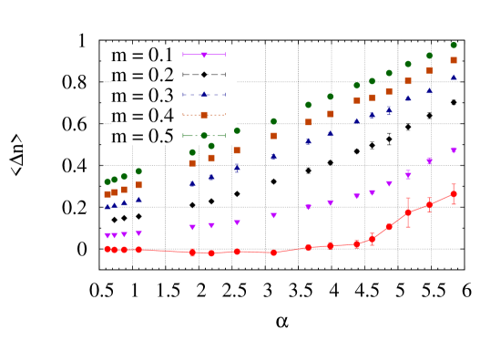
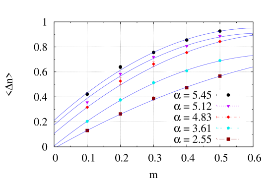
Figure 1: Phase transition of $N_{x}=N_{y}=6$ system (left figure). The red line and dots represent the $m\to 0$ extrapolated results. The right figure shows the extrapolation for a few exemplary choices of $\alpha$.

4 Conclusions and Outlook

We have demonstrated here that our code produces qualitatively the expected behavior, with a phase transition occurring at an $\alpha_{C}\approx 4$ which is not far from what was found in Ref. [9] ($\alpha_{C}\approx 3.12$). We stress that our result represents a plausibility check, not a prediction. The potential we have chosen differs from Ref. [9] and the system size is much smaller. Moreover, boundary conditions were not addressed in the same way. Very recently, there has been substantial progress in this regard: We have implemented a computation of the potential via Fast Fourier Transformation, which now allows us to simulate at larger volumes. When choosing the same potential as Ref. [9] and properly addressing boundary conditions, it appears we are now able to reproduce their results also quantitatively. We are thus confident that our code is now ready for large-scale operation.

Acknowledgements

We have benefited from discussions with Pavel Buividovich, Maxim Ulybyshev and the late Mikhail Polikarpov. This work was supported by the Deutsche Forschungsgemeinschaft within SFB 634, by the Helmholtz International Center for FAIR within the LOEWE initiative of the State of Hesse, and the European Commission, FP-7-PEOPLE-2009-RG, No. 249203. All results were obtained using Nvidia GTX and Tesla graphics cards.

References

- [1] A. H. Castro Neto et al., Rev. Mod. Phys. 81, 109 (2009); V. N. Kotov et al., Rev. Mod. Phys. 84, 1067 (2012) [arXiv:1012.3484].
- [2] V. P. Gusynin et al., Int. J. Mod. Phys. B 21 (2007) 4611 [arXiv:0706.3016].
- [3] D. C. Elias et al., Nature Phys. 7, 701 (2011) [arXiv:1104.1396]; A. S. Mayorov et al., Nano Lett. 12, 4629 (2012), [arXiv:1206.3848].
- [4] J. E. Drut and T. A. Lähde, Phys. Rev. Lett. 102, 026802 (2009) [arXiv:0807.0834]; Phys. Rev. B 79, 165425 (2009) [arXiv:0901.0584].
- [5] W. Armour, S. Hands and C. Strouthos, Phys. Rev. B 81, 125105 (2010) [arXiv:0910.5646].
- [6] R. Brower, C. Rebbi and D. Schaich, PoS LATTICE 2011, 056 (2012) [arXiv:1204.5424]; [arXiv:1101.5131].
- [7] B. Dietz, L. von Smekal et al., [arXiv:1304.4764].
- [8] P. V. Buividovich and M. I. Polikarpov, Phys. Rev. B 86, 245117 (2012) [arXiv:1206.0619].
- [9] M. V. Ulybyshev, P. V. Buividovich, M. I. Katsnelson and M. I. Polikarpov, Phys. Rev. Lett. 111, 056801 (2013) [arXiv:1304.3660].
- [10] T. O. Wehling et. al., Phys. Rev. Lett. 106, 236805 (2011) [arXiv:1101.4007].