Abstract

We consider an infinite three-dimensional waveguide that far from the coordinate origin coincides with a cylinder. The waveguide has two narrows of diameter $\varepsilon$. The narrows play the role of effective potential barriers for the longitudinal electron motion. The part of waveguide between the narrows becomes a ”resonator”  and there can arise conditions for electron resonant tunneling. A magnetic field in the resonator can change the basic characteristics of this phenomenon. In the presence of a magnetic field, the tunneling phenomenon is feasible for producing spin-polarized electron flows consisting of electrons with spins of the same direction.

We assume that the whole domain occupied by a magnetic field is in the resonator. An electron wave function satisfies the Pauli equation in the waveguide and vanishes at its boundary. Taking $\varepsilon$ as a small parameter, we derive asymptotics for the probability $T(E)$ of an electron with energy $E$ to pass through the resonator, for the ”resonant energy” $E_{res}$, where $T(E)$ takes its maximal value, and for some other resonant tunneling characteristics.

1 Introduction

In this paper, we consider a three-dimensional waveguide that, far from the coordinate origin, coincides with a cylinder $G$ containing the axis $x$. The cross-section of $G$ is a two-dimensional domain (of an arbitrary form) with smooth boundary. The waveguide has two narrows of small diameter $\varepsilon$. The waveguide part between the narrows plays the role of a resonator and there can arise conditions for electron resonant tunneling. This phenomenon consists of the fact that, for an electron with energy $E$, the probability $T(E)$ to pass from one part of the waveguide to the other through the resonator has a sharp peak at $E=E_{res}$, where $E_{res}$ denotes the ”resonant”  energy. To analyse the operation of devices based on resonant tunneling, it is important to know $E_{res}$, the behavior of $T(E)$ for $E$ close to $E_{res}$, the height of the resonant peak, etc.

The presence of a magnetic field can essentially affect the basic characteristics of the resonant tunneling and bring new possibilities for applications in electronics. In particular, in the presence of a magnetic field, the tunneling phenomenon is feasible for producing spin-polarized electron flows consisting of electrons with spins of the same direction. We suppose that a part of the resonator has been occupied by the magnetic field generated by an infinite solenoid with axis orthogonal to the axis $x$. Electron wave function satisfies the Pauli equation in the waveguide and vanishes at its boundary (the work function of the waveguide is supposed to be sufficiently large, so such a boundary condition has been justified). Moreover, we assume that only one incoming wave and one outgoing wave can propagate in each cylindrical outlet of the waveguide. In other words, we do not discuss the multichannel electron scattering and consider only electrons with energy between the first and the second thresholds. We take $\varepsilon$ as small parameter and obtain asymptotic formulas for the aforementioned characteristics of the resonant tunneling as $\varepsilon\to 0$. It turns out that such formulas depend on the limiting form of the narrows. We suppose that, in a neighborhood of each narrow, the limiting waveguide coincides with a double cone symmetric about the vertex.

The asymptotic description of electron resonant tunneling in the absence of external fields was presented in [1] for 3D quantum waveguides of similar geometry. Previously there were only episodic studies of the phenomenon by numerical methods, see [2], [3].  The extensive literature on the resonant tunneling in 1D waveguides was mainly based on the WKB-method; for our problem the method does not work. In [1], the study was based on the compound asymptotic method; the general theory of the method was elaborated in [4]. In the present paper, we modify the approach in [1] not only analysing the effect of magnetic fields but also developing a more general and simple scheme of study.

Section 2 contains statement of the problem. In Section 3, we introduce so-called ”limit” boundary value problems, which are independent of the parameter $\varepsilon$. Some model solutions to the problems are studied in Section 4. The solutions will be used in Section 5 to construct asymptotic formulas for appropriate wave functions. In the same section, we investigate the asymptotics of the wave functions and derive asymptotic formulas for main characteristics of the resonant tunneling. Remainders in the asymptotic formulas are estimated in Section 6.

2 Statement of the problem

To describe the domain $G(\varepsilon)$ in $\mathbb{R}^{3}$ occupied by the waveguide we first introduce domains $G$ and $\Omega$ in $\mathbb{R}^{3}$ independent of $\varepsilon$. The domain $G$ is the cylinder

$$G=\mathbb{R}\times D=\{(x,y,z)\in\mathbb{R}^{3}:x\in\mathbb{R}=(-\infty,+\infty);(y,z)\in D\subset\mathbb{R}^{2}\}$$

whose cross-section $D$ is a bounded two-dimensional domain with smooth boundary. Let us

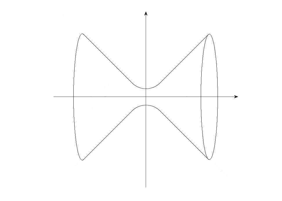
Figure 1: The domain $\Omega$.

define $\Omega$. Denote by $K$ a double cone with vertex at the coordinate origin $O$ that contains the axis $x$ and is symmetric about the origin. The set $K\cap S^{2}$ with $S^{2}$ standing for the unit sphere consists of two

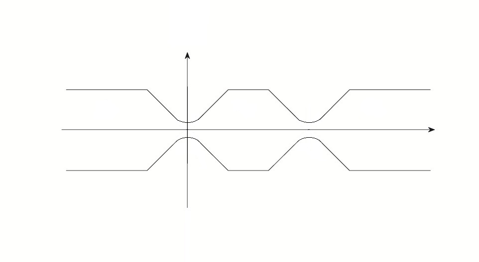
Figure 2: The waveguide $G(\varepsilon).$

non-overlapping one-connected domains symmetric about the center of sphere. Assume that the domain $\Omega$ contains the cone $K$ together with a neighborhood of its vertex. Moreover, $\Omega$ coincides with $K$ outside a sufficiently large ball centered at the origin. The boundary $\partial\Omega$ of $\Omega$ is supposed to be smooth.

Let us turn to the waveguide $G(\varepsilon)$. We denote by $\Omega(\varepsilon)$ the domain obtained from $\Omega$ by the contraction with center at $O$ and coefficient $\varepsilon$. In other words, $(x,y,z)\in\Omega(\varepsilon)$ if and only if $(x/\varepsilon,y/\varepsilon,z/\varepsilon)\in\Omega$. Let $K_{j}$ and $\Omega_{j}(\varepsilon)$ stand for $K$ and $\Omega(\varepsilon)$ shifted by the vector $\mathbf{r}_{j}=(x_{j}^{0},0,0)$, $j=1,2$. The value $|x_{1}^{0}-x_{2}^{0}|$ is assumed to be sufficiently large so that the distance between $\partial K_{1}\cap\partial K_{2}$ and $G$ is positive. We set

$$G(\varepsilon)=G\cap\Omega_{1}(\varepsilon)\cap\Omega_{2}(\varepsilon).$$

The wave function ${\bf\Psi}=(\Psi_{+},\Psi_{-})^{T}$ of an electron with energy $E=k^{2}\hbar^{2}/2m$ in a magnetic field ${\bf H_{0}}$ satisfies the Pauli equation

$$(-i\nabla+\textbf{A})^{2}{\bf\Psi}+(\widehat{\bf\sigma},\textbf{H}){\bf\Psi}=k^{2}{\bf\Psi}\quad{\text{in}}\quad G(\varepsilon),$$ (2.1)

where $\widehat{\bf\sigma}=(\sigma_{1},\sigma_{2},\sigma_{3})$ with the Pauli matrices

$$\sigma_{1}=\left(\begin{array}[]{cc}1&0\\ 0&1\\ \end{array}\right),\quad\sigma_{2}=\left(\begin{array}[]{cc}0&-i\\ i&0\\ \end{array}\right),\quad\sigma_{3}=\left(\begin{array}[]{cc}1&0\\ 0&-1\\ \end{array}\right),$$

and $\textbf{H}=-(e/c\hbar\textbf{H}_{0})=\text{rot}\,\textbf{A}$. If the magnetic field is directed along the axis $z$ that is $\textbf{H}=H\textbf{k}$, $H$ being a scalar function, then (2.1) decomposes into the two scalar equations

$$(-i\nabla+\textbf{A})^{2}\Psi_{\pm}\pm H\Psi_{\pm}=k^{2}\Psi_{\pm}.$$ (2.2)

Let the function $H$ depend only on $\rho=((x-x_{0})^{2}+(y-y_{0})^{2})^{1/2}$ with $H(\rho)=0$ for $\rho>R$, $R$ being a fixed positive number. Such a field is generated by an infinite solenoid with radius $R$ and axis parallel to the axis $z$. Then ${\bf A}=A{\bf e}_{\psi}$, where ${\bf e}_{\psi}=\rho^{-1}(-y+y_{0},x-x_{0},0)$ and

$$A(\rho)=\frac{1}{\rho}\left\{\begin{array}[]{ll}\int_{0}^{\rho}tH(t)\,dt,&\rho<R;\\ \int_{0}^{R}tH(t)\,dt,&\rho>R.\\ \end{array}\right.$$

The equality $\hbox{rot}\,\textbf{A}=\textbf{H}$ determines A up to a term of the form $\nabla f$. We neglect the waveguide boundary permeability to the electrons and consider the equations (2.2) supplemented by the homogeneous boundary condition

$$\Psi_{\pm}=0\qquad\hbox{on }\partial G(\varepsilon).$$ (2.3)

The obtained boundary value problems are self-adjoint with respect to the Green formulas

$$((-i\nabla+\textbf{A})^{2}u\pm Hu-k^{2}u,v)_{G(\varepsilon)}-(u,(-i\nabla+\textbf{A})^{2}v\pm Hv-k^{2}v)_{G(\varepsilon)}$$

$$+(u,(-\partial_{n}-A_{n})v)_{\partial G(\varepsilon)}-((-\partial_{n}-A_{n})u,v)_{\partial G(\varepsilon)}=0,$$

where $A_{n}$ is the projection of A onto the outward normal to $\partial G(\varepsilon)$ and $u,v\in C_{c}^{\infty}(G(\varepsilon))$ (which means that $u$ and $v$ are smooth functions vanishing outside a bounded set). Besides, $\Psi_{\pm}$ must satisfy some radiation conditions at infinity. To formulate such conditions, we have to introduce incoming and outgoing waves. From the requirements on H and the choice of A, it can be seen that the coefficients of equations (2.2) stabilize at infinity with a power rate. Such a slow stabilization offers difficulties in defining these waves. Therefore we will modify A by a gauge transformation so that the coefficients in (2.2) become constant for large $|x|$.

Let $(\rho,\psi)$ be polar coordinate on the plane $xy$ centered at $(x_{0},y_{0})$ and $\psi=0$ on the ray of the same direction as the axis $x$. We introduce $f(x,y,z)=c\psi$, where $c=\int_{0}^{R}tH(t)\,dt$. For definiteness, assume that $-\pi/2<\psi<3\pi/2$. The function $f$ is uniquely determined in the waveguide for $|x-x_{0}|>0$, moreover, $\nabla f=\textbf{A}$ for $|x-x_{0}|>R$. Let $\tau$ be a cut-off function on $\mathbb{R}_{+}$ equal to $1$ for $t>R+2$ and $0$ for $t<R+1$. We set $\textbf{A}^{\prime}(x,y,z)=\textbf{A}(x,y,z)-\nabla(\tau(|x-x_{0}|)f(x,y,z))$. Then $\hbox{rot}\,\textbf{A}^{\prime}=\hbox{rot}\,\textbf{A}=\textbf{H}$ while $\textbf{A}^{\prime}=0$ for $|x-x_{0}|>R+2$. The wave functions $\Psi_{\pm}^{\prime}=\Psi_{\pm}\exp\{i\tau f\}$ satisfy (2.2) with A replaced by $\textbf{A}^{\prime}$. For $|x-x_{0}|>R+2$, the coefficients of the equations (2.2) with new vector potential $\textbf{A}^{\prime}$ coincide with the coefficients of the Helmholtz equation

$$-\triangle\Psi_{\pm}^{\prime}=k^{2}\Psi_{\pm}^{\prime}.$$

In order to formulate the radiation conditions, we consider the problem

$$\Delta v(y,z)+\lambda^{2}v(y,z) = 0,\qquad(y,z)\in D,$$ (2.4)

$$v(y,z) = 0,\qquad(y,z)\in\partial D.$$

The values of parameter $\lambda^{2}$ that correspond to the nontrivial solutions of this problem form the sequence $\lambda^{2}_{1}<\lambda^{2}_{2}<\dots$ with $\lambda^{2}_{1}>0$. These numbers are called the thresholds. Assume that $k^{2}$ in (2.2) coincides with none of the thresholds and take up the equation in (2.2) with $\Psi_{+}$. For a fixed $k^{2}>\lambda_{1}^{2}$ there exist finitely many bounded solutions (wave functions) linearly independent modulo $L_{2}(G(\varepsilon))$; in other words, a linear combination of such solutions belongs to $L_{2}(G(\varepsilon))$ if and only if all coefficients are equal to zero. The number of wave functions with such properties remains constant for $k^{2}\in(\lambda^{2}_{q},\lambda^{2}_{q+1})$, $q=1,2,\dots$ and step-wise increases at the thresholds.

In the present paper, we discuss only the situation, where $k^{2}\in(\lambda^{2}_{1},\lambda^{2}_{2})$. In such a case, there exist two independent wave functions. A basis in the space spanned by such functions can be composed of the wave functions $u^{+}_{1}$ and $u^{+}_{2}$ satisfying the radiation conditions

$$u_{1}^{+}(x,y,z) = \begin{cases}e^{i\nu_{1}x}\Psi_{1}(y,z)+s_{11}^{+}(k)\,e^{-i\nu_{1}x}\Psi_{1}(y,z)+O(e^{\delta x}),&x\rightarrow-\infty,\\ s_{12}^{+}(k)\,e^{i\nu_{1}x}\Psi_{1}(y,z)+O(e^{-\delta x}),&x\rightarrow+\infty;\\ \end{cases}$$ (2.5)

$$u_{2}^{+}(x,y) = \begin{cases}s_{21}^{+}(k)\,e^{-i\nu_{1}x}\Psi_{1}(y,z)+O(e^{\delta x}),&x\rightarrow-\infty,\\ e^{-i\nu_{1}x}\Psi_{1}(y,z)+s_{22}^{+}(k)\,e^{i\nu_{1}x}\Psi_{1}(y,z)+O(e^{-\delta x}),&x\rightarrow+\infty;\\ \end{cases}$$

here $\nu_{1}=\sqrt{k^{2}-\lambda^{2}_{1}}$ and $\Psi_{1}$ stands for an eigenfunction of problem (2.4) corresponding to $\lambda^{2}_{1}$ and being normalized by the equality

$$\nu_{1}\int_{D}|\Psi_{1}(y,z)|^{2}\,dy\,dz=1.$$ (2.6)

The function $U_{1}(x,y,z)=e^{i\nu_{1}x}\Psi_{1}(y,z)$ in the cylinder $G$ is a wave incoming from $-\infty$ and outgoing to $+\infty$, while $U_{2}(x,y,z)=e^{-i\nu_{1}x}\Psi_{1}(y,z)$ is a wave going from $+\infty$ to $-\infty$. The matrix

$$S^{+}=\|s_{mj}^{+}\|_{m,j=1,2}$$

with entries determined by (2.5) is called the scattering matrix; it is unitary. The quantities

$$R_{1}^{+}:=|s_{11}^{+}|^{2},\qquad\,\,\,T_{1}^{+}:=|s_{1\,2}^{+}|^{2}$$

are called the reflection coefficient and the transition coefficient for the wave $U_{1}$ coming in $G(\varepsilon)$ from $-\infty$. (Similar definitions can be given for the wave $U_{2}$, incoming from $+\infty$.) In the same manner we introduce the scattering matrix $S^{-}$ and the reflection and transition coefficients $R^{-}_{1}$ and $T^{-}_{1}$ for the equation in (2.2) with $\Psi_{-}$.

We consider only the scattering of the wave going from $-\infty$ and denote the reflection and transition coefficients by

$$R^{\pm}=R^{\pm}(k,\varepsilon)=|s_{11}^{\pm}(k,\varepsilon)|^{2},\qquad\,\,\,T^{\pm}=T^{\pm}(k,\varepsilon)=|s_{12}^{\pm}(k,\varepsilon)|^{2}.$$ (2.7)

We intend to find a ”resonant”  value $k_{r}^{\pm}=k_{r}^{\pm}(\varepsilon)$ of the parameter $k$ which corresponds to the maximum of the transition coefficient and to describe the behavior of $T^{\pm}(k,\varepsilon)$ near $k_{r}^{\pm}(\varepsilon)$ as $\varepsilon\to 0$.

3 Limit problems

To derive the asymptotics of a wave function (i.e. a solution to problem (2.2)) as $\varepsilon\rightarrow 0$, we make use of the compound asymptotics method. To this end, we introduce the ”limit”  problems independent of $\varepsilon$. Let the vector potential $\textbf{A}^{\prime}$ and, in particular, the magnetic field $H$ differ from zero only in the resonator, which is the part of waveguide between the narrows. Then, outside the resonator and in a neighborhood of the narrows, the wave function under consideration satisfies the Helmholtz equation.

3.1 First kind limit problems

We set $G(0)=G\cap K_{1}\cap K_{2}$ (Fig. 3), so $G(0)$ consists of three parts $G_{1}$, $G_{2}$, and $G_{3}$.

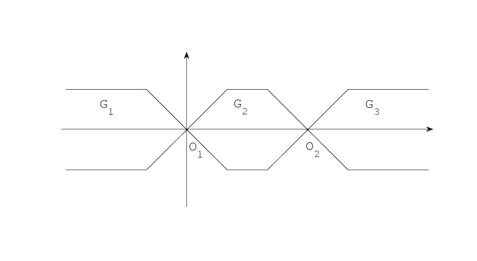
Figure 3: The domain $G(0).$

The boundary value problems

$$\Delta v(x,y,z)+k^{2}v(x,y,z) = f(x,y,z),\qquad(x,y,z)\in G_{j},$$ (3.1)

$$v(x,y,z) = 0,\qquad(x,y,z)\in\partial G_{j},$$

where $j=1,3$, and

$$(-i\nabla+\textbf{A}^{\prime})^{2}v(x,y,z)\pm H(\rho)v(x,y,z)-k^{2}v(x,y,z) = f(x,y,z),\quad(x,y,z)\in G_{2},\qquad$$ (3.2)

$$v(x,y,z) = 0,\qquad(x,y,z)\in\partial G_{2},$$

are called the first kind limit problems.

We introduce function spaces for the problem (3.2) in $G_{2}$. Denote by $O_{1}$ and $O_{2}$ the conical points of the boundary $\partial G_{2}$ and by $\phi_{1}$ and $\phi_{2}$ smooth real functions on the closure $\overline{G_{2}}$ of $G_{2}$ such that $\phi_{j}=1$ in a neighborhood of $O_{j}$ while $\phi_{1}^{2}+\phi_{2}^{2}=1$. For $l=0,1,2$ and $\gamma\in\mathbb{R}$, we denote by $V^{l}_{\gamma}(G_{2})$ the completion in the norm

$$\|v;V^{l}_{\gamma}(G_{2})\|=\left(\int_{G_{2}}\sum_{|\alpha|=0}^{l}\sum_{j=1}^{2}\phi_{j}^{2}(x,y,z)r_{j}^{2(\gamma-l+|\alpha|)}|\partial^{\alpha}v(x,y,z)|^{2}\,dx\,dy\,dz\right)^{1/2}$$ (3.3)

of the set of smooth functions on $\overline{G_{2}}$ vanishing near $O_{1}$ and $O_{2}$; here $r_{j}$ is the distance between the points $(x,y,z)$ and $O_{j}$, $\alpha=(\alpha_{1},\alpha_{2},\alpha_{3})$ is the multiindex, and $\partial^{\alpha}=\partial^{|\alpha|}/\partial x^{\alpha_{1}}\partial y^{\alpha_{2}}\partial z^{\alpha_{3}}$.

Let $K_{j}$ be the tangent cone to $\partial G_{2}$ at $O_{j}$ and $S(K_{j})$ the domain that $K_{j}$ cuts out on the unit sphere centered at $O_{j}$. We denote by $\mu_{1}(\mu_{1}+1)$ and $\mu_{2}(\mu_{2}+1)$ the first and second eigenvalues of the Dirichlet problem for the Laplace-Beltrami operator in $S(K_{1})$, $0<\mu_{1}(\mu_{1}+1)<\mu_{2}(\mu_{2}+1)$. Moreover, let $\Phi_{1}$ stand for an eigenfunction corresponding to $\mu_{1}(\mu_{1}+1)$ and normalized by

$$(2\mu_{1}+1)\int_{S(K_{1})}|\Phi_{1}(\varphi)|^{2}d\varphi=1.$$

The next proposition follows from the general results, e.g. see [5, Chapters 2 and 4, §§1–3] or [4, v. 1, Chapter 1].

Proposition 3.1.

Assume that $|\gamma-1|<\mu_{1}+1/2$. Then for $f\in V^{0}_{\gamma}(G_{2})$ and any $k^{2}$ except the positive increasing sequence $\{k^{2}_{p}\}_{p=1}^{\infty}$ of eigenvalues $k^{2}_{p}\to\infty$, there exists a unique solution $v\in V^{2}_{\gamma}(G_{2})$ to the problem (3.2) in $G_{2}$. The estimate

$$\|v;V^{2}_{\gamma}(G_{2})\|\leq c\|f;V^{0}_{\gamma}(G_{2})\|$$ (3.4)

holds with a constant $c$ independent of $f$. If $f$ vanishes in a neighborhood of $O_{1}$ and $O_{2}$, then $v$ admits the asymptotics

$$v(x,y,z)=\left\{\begin{array}[]{ll}b_{1}r_{1}^{-1/2}\widetilde{J}_{\mu_{1}+1/2}(kr_{1})\Phi_{1}(\varphi_{1})+O\bigl{(}r_{1}^{\mu_{2}+1/2}\bigr{)},&\hbox{$r_{1}\rightarrow 0$;}\\ b_{2}r_{2}^{-1/2}\widetilde{J}_{\mu_{1}+1/2}(kr_{2})\Phi_{1}(-\varphi_{2})+O\bigl{(}r_{2}^{\mu_{2}+1/2}\bigr{)},&\hbox{$r_{2}\rightarrow 0$}\\ \end{array}\right.$$

near $O_{1}$ and $O_{2}$, where $(r_{j},\varphi_{j})$ are ”polar coordinates” centered at $O_{j}$, $r_{j}>0$ and and $\varphi_{j}\in S(K_{j})$; $b_{j}$ are certain constants; $\widetilde{J}_{\mu}$ denotes the Bessel function multiplied by a constant such that $\widetilde{J}_{\mu}(kr)=r^{\mu}+o(r^{\mu})$.

Let $k^{2}=k^{2}_{0}$ be an eigenvalue of problem (3.2), then the problem (3.2) is solvable if and only if $(f,v_{0})_{G_{2}}=0$ for any eigenfunction $v_{0}$ corresponding to $k^{2}_{0}$. Under such conditions there exists a unique solution $v$ to problem (3.2) that is orthogonal to all these eigenfunctions and satisfies (3.4).

We turn to problems (3.1) for $j=1,3$. Let $\chi_{0,j}$ and $\chi_{\infty,j}$ be smooth real functions on the closure $\overline{G}_{j}$ of $G_{j}$ such that $\chi_{0,j}=1$ in a neighborhood of $O_{j}$, $\chi_{0,j}=0$ outside a compact set, and $\chi_{0,j}^{2}+\chi_{\infty,j}^{2}=1$. We also assume that the support ${\rm supp}\chi_{\infty,j}$ is in the cylindrical part of $G_{j}$. For $\gamma\in\mathbb{R}$, $\delta>0$, and $l=0,1,2$, the space $V^{l}_{\gamma,\,\delta}(G_{j})$ is the completion in the norm

$$\|v;V^{l}_{\gamma,\,\delta}(G_{j})\|=\left(\int_{G_{j}}\sum_{|\alpha|=0}^{l}\,\bigl{(}\chi_{0,j}^{2}r_{j}^{2(\gamma-l+|\alpha|)}+\chi_{\infty,j}^{2}\exp(2\delta x)\bigr{)}|\partial^{\alpha}v|^{2}\,dx\,dy\,dz\right)^{1/2}$$ (3.5)

of the set of functions with compact support smooth on $\overline{G}_{j}$ and equal to zero in a neighborhood of $O_{j}$.

By assumption, $k^{2}$ is between the first and second thresholds, so in every domain $G_{j}$ there is only one outgoing wave; let $U_{1}^{-}=U_{2}$ be the outgoing wave in $G_{1}$ and $U_{2}^{-}=U_{1}$ that in $G_{3}$ (the definition of the waves $U_{j}$ in $G$ see in Section 2). The next proposition follows from Theorem 5.3.5 in [5].

Proposition 3.2.

Let $|\gamma-1|<\mu_{1}+1/2$ and let the homogeneous problem (3.1) (with $f=0$) have no nontrivial solutions in $V^{2}_{\gamma,\,0}(G_{j})$. Then for any right-hand side $f\in V^{0}_{\gamma,\,\delta}(G_{j})$ there exists a unique solution $v$ to the problem (3.1) that admits the representation

$$v=u+A_{j}\chi_{\infty,j}U^{-}_{j},$$

where $A_{j}=const$, $u\in V^{2}_{\gamma,\,\delta}(G_{j})$ and $\delta$ is sufficiently small. Moreover there holds the estimate

$$\|u;V^{2}_{\gamma,\,\delta}(G_{j})\|+|A_{j}|\leq c\|f;V^{0}_{\gamma,\,\delta}(G_{j})\|,$$ (3.6)

with a constant $c$ independent of $f$. If the function $f$ vanishes in a neighborhood of $O_{j}$, then the solution $v$ in $G_{1}$ admits the decomposition

$$v(x,y,z)=a_{1}r_{1}^{-1/2}\widetilde{J}_{\mu_{1}+1/2}(kr_{1})\Phi_{1}(-\varphi_{1})+O\big{(}r_{1}^{\mu_{2}+1/2}\big{)},\quad r_{1}\rightarrow 0,$$

and for the solution in $G_{3}$ there holds

$$v(x,y)=a_{2}r_{2}^{-1/2}\widetilde{J}_{\mu_{1}+1/2}(kr_{2})\Phi_{1}(\varphi_{2})+O\big{(}r_{2}^{\mu_{2}+1/2}\big{)},\quad r_{2}\rightarrow 0,$$

where $a_{j}$ are certain constants and $\mu_{l}$ are the same as in the preceding proposition.

3.2 Second kind limit problems.

In the domains $\Omega_{j}$, $j=1,2$, introduced in Section 2, we consider the boundary value problems

$$\triangle w(\xi_{j},\eta_{j},\zeta_{j})=F(\xi_{j},\eta_{j},\zeta_{j}),\quad(\xi_{j},\eta_{j},\zeta_{j})\in\Omega_{j};\qquad w(\xi_{j},\eta_{j},\zeta_{j})=0,\quad(\xi_{j},\eta_{j},\zeta_{j})\in\partial\Omega_{j},$$ (3.7)

which are called the second kind limit problems; here $(\xi_{j},\eta_{j},\zeta_{j})$ denote Cartesian coordinates with origin at  $O_{j}$.

Let $\rho_{j}={\rm dist}((\xi_{j},\eta_{j},\zeta_{j}),O_{j})$ and let $\psi_{0,j}$, $\psi_{\infty,j}$ be smooth real functions on $\overline{\Omega}_{j}$ such that $\psi_{0,j}=1$ for $\rho_{j}<N/2$, $\psi_{0,j}=0$ for $\rho_{j}>N$, and $\psi_{0,j}^{2}+\psi_{\infty,j}^{2}=1$ with sufficiently large positive $N$. For $\gamma\in\mathbb{R}$ and $l=0,1,2$, the space $V^{l}_{\gamma}(\Omega_{j})$ is the completion in the norm

$$\|v;V^{l}_{\gamma}(\Omega_{j})\|=\left(\int_{\Omega_{j}}\sum_{|\alpha|=0}^{l}\,\bigl{(}\psi_{0,j}^{2}+\psi_{\infty,j}^{2}\rho_{j}^{2(\gamma-l+|\alpha|)}\bigr{)}|\partial^{\alpha}v|^{2}\,d\xi_{j}d\eta_{j}d\zeta_{j}\right)^{1/2}$$ (3.8)

of the set $C^{\infty}_{c}(\overline{\Omega}_{j})$ of smooth functions with compact support in $\overline{\Omega}_{j}$. The next proposition is a corollary of Theorem 4.3.6 in [5].

Proposition 3.3.

Assume that $|\gamma-1|<\mu_{1}+1/2$. Then for $F\in V^{0}_{\gamma}(\Omega_{j})$ there exists a unique solution $w\in V^{2}_{\gamma}(\Omega_{j})$ of the problem (3.7) such that

$$\|w;V^{2}_{\gamma}(\Omega_{j})\|\leq c\|F;V^{0}_{\gamma}(\Omega_{j})\|,$$ (3.9)

with a constant $c$ independent of $F$. If $F\in C^{\infty}_{c}(\overline{\Omega}_{j})$, then the function $w$ is smooth on $\overline{\Omega}_{j}$ and admits the representation

$$w(\xi_{j},\eta_{j},\zeta_{j})=\begin{cases}\alpha_{j}\rho_{j}^{-\mu_{1}-1}\Phi_{1}(-\varphi_{j})+O\bigl{(}\rho_{j}^{-\mu_{2}-1}\bigr{)},&\xi_{j}<0,\\ \beta_{j}\rho_{j}^{-\mu_{1}-1}\Phi_{1}(\varphi_{j})+O\bigl{(}\rho_{j}^{-\mu_{2}-1}\bigr{)},&\xi_{j}>0,\end{cases}$$ (3.10)

with $\rho_{j}\rightarrow\infty$; here $(\rho_{j},\varphi_{j})$ are polar coordinates on $\Omega_{j}$ centered at $O_{j}$ while $\mu_{l}$ and $\Phi_{1}$ are the same as in Proposition  3.1. The constants $\alpha_{j}$ and $\beta_{j}$ are given by

$$\alpha_{j}=-(F,w_{j}^{l})_{\Omega},\qquad\beta_{j}=-(F,w_{j}^{r})_{\Omega},$$

where $w_{j}^{l}$ and $w_{j}^{r}$ are unique solutions to the homogeneous problem (3.7) that satisfy, for $\rho_{j}\to\infty$, the conditions

$$w_{j}^{l}=\begin{cases}\left(\rho_{j}^{\mu_{1}}+\alpha\rho_{j}^{-\mu_{1}-1}\right)\Phi_{1}(-\varphi_{j})+O\bigl{(}\rho_{j}^{-\mu_{2}-1}\bigr{)},&\xi_{j}<0;\\ \beta\rho_{j}^{-\mu_{1}-1}\Phi_{1}(\varphi_{j})+O\bigl{(}\rho_{j}^{-\mu_{2}-1}\bigr{)},&\xi_{j}>0;\end{cases}$$ (3.11)

$$w_{j}^{r}=\begin{cases}\beta\rho_{j}^{-\mu_{1}-1}\Phi_{1}(-\varphi_{j})+O\bigl{(}\rho_{j}^{-\mu_{2}-1}\bigr{)},&\xi_{j}<0;\\ \left(\rho_{j}^{\mu_{1}}+\alpha\rho_{j}^{-\mu_{1}-1}\right)\Phi_{1}(\varphi_{j})+O\bigl{(}\rho_{j}^{-\mu_{2}-1}\bigr{)},\qquad&\xi_{j}>0.\end{cases}$$ (3.12)

The coefficients $\alpha$ and $\beta$ depend only on the domain $\Omega$.

4 Special solutions of limit problems

In each domain $G_{j}$, $j=1,2,3$, we introduce special solutions to the homogeneous problems (3.1). Such solutions will be needed in the next section for constructing the asymptotics of a wave function. From Propositions 3.1 and 3.2 it follows that the bounded solutions of the homogeneous problems (3.1) are trivial (except the eigenfunctions of the problem in $G_{2}$), so we will consider solutions unbounded in a neighborhoods of the points $O_{j}$.

Let us consider the problem in the cone $K_{1}$, which is, as in Proposition  3.1, the tangent cone to $\partial G_{2}$ at $O_{1}$:

$$\Delta u+k^{2}u=0\,\,\mbox{in}\,K,\qquad u=0\,\,\mbox{on}\,\,\partial K.$$ (4.1)

The function

$$v(r,\varphi)=r^{-1/2}\widetilde{N}_{\mu+1/2}(kr)\Phi_{1}(\varphi)$$ (4.2)

satisfies problem (4.1); here $\widetilde{N}_{\mu}$ is the Neumann function multiplied by such a constant that

$$\widetilde{N}_{\mu}(kr)=r^{-\mu}+o(r^{-\mu}),$$

and $\Phi_{1}$ is the same function as in Proposition  3.1. Let $t\mapsto\Theta(t)$ be a cut-off function on $\mathbb{R}$ equal to  1 for $t<\delta/2$ and  0 for $t>\delta$ with a small positive $\delta$. We introduce the solution

$$\textbf{v}_{1}(x,y,z)=\Theta(r_{1})v(r_{1},\varphi_{1})+\widetilde{v}_{1}(x,y,z)$$ (4.3)

to the homogeneous problem (3.1) in $G_{1}$, whereas $\widetilde{v}_{1}$ satisfies (3.1) with $f=-[\triangle,\Theta]v$; the existence of $\widetilde{v}_{1}$ is provided by Proposition  3.2. Thus

$$\textbf{v}_{1}(x,y,z)=\begin{cases}r_{1}^{-1/2}\bigl{(}\widetilde{N}_{\mu_{1}+1/2}(kr_{1})+a\widetilde{J}_{\mu_{1}+1/2}(kr_{1})\bigr{)}\Phi_{1}(-\varphi_{1})+O(r_{1}^{\mu_{2}}),&r_{1}\rightarrow 0,\\ AU_{1}^{-}(x,y,z)+O(e^{\delta x}),\quad x\rightarrow-\infty,&\\ \end{cases}$$ (4.4)

where $\widetilde{J}_{\mu}$ is the same function as in Proposition  3.1 and  3.2 and the constant $A\neq 0$ depends only on the domain $G_{1}$.

In the domain $G_{3}$, we introduce the solution $\textbf{v}_{3}$ to the homogeneous problem (3.1), $\textbf{v}_{3}(x,y,z):=\textbf{v}_{1}(d-x,-y,-z)$, where $d=\mbox{dist}(O_{1},O_{2})$. Then

$$\textbf{v}_{3}(x,y,z)=\begin{cases}r_{2}^{-1/2}\bigl{(}\widetilde{N}_{\mu_{1}+1/2}(kr_{2})+a\widetilde{J}_{\mu_{1}+1/2}(kr_{2})\bigr{)}\Phi_{1}(\varphi_{2})+O(r_{2}^{\mu_{2}}),&r_{2}\rightarrow 0,\\ Ae^{-i\nu_{1}d}U_{2}^{-}(x,y,z)+O(e^{-\delta x}),\quad x\rightarrow+\infty.&\\ \end{cases}$$ (4.5)

Lemma 4.1.

There holds the equality $|A|^{2}={\rm Im}\,a$.

Proof.

Let $(u,v)_{Q}$ stand for the integral $\int_{Q}u\overline{v}\,dx\,dy\,dz$, and let $G_{N,\,\delta}$ be the truncated domain $G_{1}\cap\{x>-N\}\cap\{r_{1}>\delta\}$. By the Green formula

$$0=(\triangle\textbf{v}_{1}+k^{2}\textbf{v}_{1},\textbf{v}_{1})_{G_{N,\,\delta}}-(\textbf{v}_{1},\triangle\textbf{v}_{1}+k^{2}\textbf{v}_{1})_{G_{N,\,\delta}}$$

$$=(\partial\textbf{v}_{1}/\partial n,\textbf{v}_{1})_{\partial G_{N,\,\delta}}-(\textbf{v}_{1},\partial\textbf{v}_{1}/\partial n)_{\partial G_{N,\,\delta}}=2i\,{\rm Im}\,(\partial\textbf{v}_{1}/\partial n,\textbf{v}_{1})_{E},$$

where $E=(\partial G_{N,\,\delta}\cap\{x=-N\})\cup(\partial G_{N,\,\delta}\cap\{r_{1}=\delta\})$. Taking into account (4.4) for $x\rightarrow+\infty$ and (2.6), we have

$${\rm Im}\,(\partial\textbf{v}_{1}/\partial n,\textbf{v}_{1})_{\partial G_{N,\,\delta}\cap\{x=-N\}}=-{\rm Im}\,\int_{D}A\dfrac{\partial U_{1}^{-}}{\partial x}(x,y,z)\overline{AU_{1}^{-}}(x,y,z)\Big{|}_{x=-N}dy\,dz+o(1)$$

$$=|A|^{2}\nu_{1}\int_{-l/2}^{l/2}|\Psi_{1}(y,z)|^{2}dy\,dz+o(1)=|A|^{2}+o(1).$$

With (4.4) as $r_{1}\rightarrow 0$ and the definition of $\Phi_{1}$ (see Proposition  3.1), we obtain

$${\rm Im}\,(\partial\textbf{v}_{1}/\partial n,\textbf{v}_{1})_{\partial G_{N,\,\delta}\cap\{r_{1}=\delta\}}={\rm Im}\int_{S(K)}\,\biggl{[}-\dfrac{\partial}{\partial r_{1}}r_{1}^{-1/2}\bigl{(}\widetilde{N}_{\mu_{1}+1/2}(kr_{1})+a\widetilde{J}_{\mu_{1}+1/2}(kr_{1})\bigr{)}\biggr{]}$$

$$\times r_{1}^{-1/2}\bigl{(}\widetilde{N}_{\mu_{1}+1/2}(kr_{1})+\overline{a}\widetilde{J}_{\mu_{1}+1/2}(kr_{1})\bigr{)}|\Phi_{1}(-\varphi_{1})|^{2}r_{1}^{2}\Big{|}_{r_{1}=\delta}d\varphi_{1}+o(1)$$

$$=-({\rm Im}\,a)(2\mu_{1}+1)\int_{S(K)}|\Phi(-\varphi_{1})|^{2}d\varphi_{1}+o(1)=-{\rm Im}\,a+o(1).$$

Thus $|A|^{2}-{\rm Im}\,a+o(1)=0$ as $N\rightarrow\infty$ and $\delta\rightarrow 0$.  ∎

Let $k^{2}_{0,\pm}$ be a simple eigenvalue of the problem (3.2) in the resonator $G_{2}$ and $v_{0}^{\pm}$ is an eigenfunction corresponding to $k^{2}_{0,\pm}$ and normalized by the condition $\int_{G_{2}}|v_{0}^{\pm}|^{2}dx\,dy\,dz=1$. By virtue of Proposition  3.1

$$v_{0}^{\pm}(x,y,z)\sim\begin{cases}b_{1}^{\pm}r_{1}^{-1/2}\widetilde{J}_{\mu_{1}+1/2}(k_{0,\pm}r_{1})\Phi(\varphi_{1}),&r_{1}\rightarrow 0,\\ b_{2}^{\pm}r_{2}^{-1/2}\widetilde{J}_{\mu_{1}+1/2}(k_{0,\pm}r_{2})\Phi(-\varphi_{2}),&r_{2}\rightarrow 0.\\ \end{cases}$$ (4.6)

We consider that $b_{j}^{\pm}\neq 0$. If $H=0$, then it is true, for instance, for the eigenfunctions corresponding to the minimal eigenvalue of the resonator. For nonzero $H$ this condition can be violated owing to the Aharonov-Bohm effect; here we do not discuss this phenomenon. For $k^{2}$ in a punctured neighborhood of $k^{2}_{0,\pm}$ separated from the other eigenvalues, we introduce the solutions $v_{0j}^{\pm}$ to the homogeneous problem (3.2) by the relations

$$v_{0j}^{\pm}(x,y,z)=\Theta(r_{j})v(r_{j},\varphi_{j})+\widetilde{v}_{0j}^{\pm}(x,y,z),\qquad j=1,2,$$ (4.7)

where $v$ is defined by (4.2) and $\widetilde{v}_{0j}^{\pm}$ is a bounded solution to the problem (3.2) with $f_{j}(x,y,z)=-[\triangle,\Theta(r_{j})]v(r_{j},\varphi_{j})$.

Lemma 4.2.

In a neighborhood $V\subset\mathbb{C}$ of $k^{2}_{0,\pm}$ containing no eigenvalues of the problem (3.2) in $G_{2}$ distinct from $k^{2}_{0,\pm}$, there hold the equalities $\widetilde{v}_{0j}^{\pm}=-\overline{b_{j}^{\pm}}(k^{2}-k^{2}_{0,\pm})^{-1}v_{0}^{\pm}+\widehat{v}_{0j}^{\pm}$, where $b_{j}^{\pm}$ are the same as in (4.6) and the functions $\widehat{v}_{0j}^{\pm}$ are analytic in $k^{2}\in V$.

Proof.

We first verify that $(v_{0j}^{\pm},v_{0}^{\pm})_{G_{2}}=-\overline{b_{j}^{\pm}}/(k^{2}-k^{2}_{0,\pm})$, where $v_{0j}^{\pm}$ are defined by (4.7). We have

$$(\triangle v_{0j}^{\pm}+k^{2}v_{0j}^{\pm},v_{0}^{\pm})_{G_{\delta}}-(v_{0j}^{\pm},\triangle v_{0}^{\pm}+k^{2}v_{0}^{\pm})_{G_{\delta}}=-(k^{2}-k^{2}_{0,\pm})(v_{0j}^{\pm},v_{0}^{\pm})_{G_{\delta}};$$

the domain $G_{\delta}$ is obtained from $G_{2}$ by cutting out the balls of radius $\delta$ with centers at $O_{1}$ and $O_{2}$. Applying the Green formula in the same way as in the proof of Lemma  4.1, we arrive at $-(k^{2}-k^{2}_{0,\pm})(v_{0j}^{\pm},v_{0}^{\pm})_{G_{\delta}}=\overline{b_{j}^{\pm}}+o(1)$. It remains to let $\delta\to 0$.

Since $k^{2}_{0,\pm}$ is a simple eigenvalue, we have

$$\widetilde{v}_{0j}^{\pm}=\frac{B_{j}^{\pm}(k^{2})}{k^{2}-k^{2}_{0,\pm}}v_{0}^{\pm}+\widehat{v}_{0j}^{\pm},$$ (4.8)

where $B_{j}^{\pm}(k^{2})$ is independent of $(x,y,z)$ and $\widehat{v}_{0j}^{\pm}$ are certain functions analytic in $k^{2}$ near $k^{2}=k^{2}_{0,\pm}$. Multiplying (4.7) by $v_{0}^{\pm}$ and taking into account (4.8), the obtained function for $(v_{0j}^{\pm},v_{0}^{\pm})_{G_{2}}$, and the normalized condition $(v_{0}^{\pm},v_{0}^{\pm})_{G_{2}}=1$, we arrive at $B_{j}^{\pm}(k^{2})=-\overline{b_{j}^{\pm}}+(k^{2}-k^{2}_{0,\pm})\widetilde{B}_{j}^{\pm}(k^{2})$, $\widetilde{B}_{j}^{\pm}$ are being certain analytic functions. Together with (4.8), this completes the proof.   ∎

In view of Lemma  4.2, the expressions $\mbox{{\bf v}}_{21}^{\pm}=(k^{2}-k^{2}_{0,\pm})v_{01}^{\pm}$ and ${\bf v}_{22}^{\pm}=\overline{b_{2}^{\pm}}v_{01}-\overline{b_{1}^{\pm}}v_{02}^{\pm}$ can be extended by continuity to $k^{2}_{0,\pm}$. According to Proposition 3.1,

$$\textbf{v}_{21}^{\pm}(x,y) \sim\begin{cases}r_{1}^{-1/2}\bigl{(}(k^{2}-k^{2}_{0,\pm})\widetilde{N}_{\mu_{1}+1/2}(kr_{1})+c_{1}^{\pm}(k)\widetilde{J}_{\mu_{1}+1/2}(kr_{1})\bigr{)}\Phi_{1}(\varphi_{1}),&r_{1}\rightarrow 0,\\ c_{2}^{\pm}(k)r_{2}^{-1/2}\widetilde{J}_{\mu_{1}+1/2}(kr_{2})\Phi_{1}(-\varphi_{2}),&r_{2}\rightarrow 0,\\ \end{cases}$$ (4.9)

$$\textbf{v}_{22}^{\pm}(x,y) \sim\begin{cases}r_{1}^{-1/2}\bigl{(}\overline{b_{2}^{\pm}}\widetilde{N}_{\mu_{1}+1/2}(kr_{1})+d_{1}^{\pm}(k)\widetilde{J}_{\mu_{1}+1/2}(kr_{1})\bigr{)}\Phi_{1}(\varphi_{1}),&r_{1}\rightarrow 0,\\ r_{2}^{-1/2}\bigl{(}-\overline{b_{1}^{\pm}}\widetilde{N}_{\mu_{1}+1/2}(kr_{2})+d_{2}^{\pm}(k)\widetilde{J}_{\mu_{1}+1/2}(kr_{2})\bigr{)}\Phi_{1}(-\varphi_{2}),&r_{2}\rightarrow 0.\\ \end{cases}$$ (4.10)

From the proof of Lemma 4.2 it follows that $c_{j}^{\pm}(k_{0,\pm})=-\overline{b_{1}^{\pm}}b_{j}^{\pm}$.

5 Asymptotic formulas

In Section 5.1, we present an asymptotic formula for a wave function (see (5.1)), explain its structure, and describe the solutions of the first kind limit problems involved in the formula. We complete deriving the formula (5.1) in 5.2, where we describe the involved solutions of the second kind limit problems and calculate some coefficients in the expressions for the solutions of the first kind problems. In Section 5.3, when analysing the expression for $\widetilde{s}_{12}$ obtained in 5.2, we derive formal asymptotics of the resonant tunneling characteristics. Note that the remainders in (5.20) – (5.22) have arisen at the intermediate stage of consideration during simplification of the principal part of the asymptotics; they are not the remainders in the final asymptotic formulas. The ”final”  remainders are estimated in the next Section 6, see Theorem 6.3. First, we derive the integral estimate (6.13) of the remainder in (5.1), which proves to be sufficient to obtain more simplified estimates of the remainders in the formulas for the characteristics of resonant tunneling. The formula (5.1) and the estimate (6.13) are auxiliary and are analysed only to that extent, which is needed for deriving the asymptotics of tunneling. For ease of notations, we shall in this section drop the symbol ”$\pm$”, meaning that we deal with one of the equations (2.2).

5.1 The asymptotics of a wave function

In the waveguide $G(\varepsilon)$, we consider the scattering of the wave $U(x,y,z)=e^{i\nu_{1}x}\Psi_{1}(y,z)$ incoming from $-\infty$ (see (2.6)). The corresponding wave function admits the representation

$$u(x,y,z;\varepsilon)=\chi_{1,\,\varepsilon}(x,y,z)v_{1}(x,y,z;\varepsilon)+$$

$$+\Theta(r_{1})w_{1}(\varepsilon^{-1}x_{1},\varepsilon^{-1}y_{1},\varepsilon^{-1}z_{1};\varepsilon)+\chi_{2,\,\varepsilon}(x,y,z)v_{2}(x,y,z;\varepsilon)+$$ (5.1)

$$+\Theta(r_{2})w_{2}(\varepsilon^{-1}x_{2},\varepsilon^{-1}y_{2},\varepsilon^{-1}z_{2};\varepsilon)+\chi_{3,\,\varepsilon}(x,y,z)v_{3}(x,y,z;\varepsilon)+R(x,y,z;\varepsilon).$$

Let us explain the notation and structure of this formula. When constructing the asymptotics, we first describe the behavior of the wave function $u$ outside the narrows approximating $u$ by the solutions $v_{j}$ of the homogeneous problems (3.1) and (3.2) in $G_{j}$. As $v_{j}$ we take certain linear combinations of the special solutions introduced in the preceding section; in doing so we subject $v_{1}$ and $v_{3}$ to the same radiation conditions at infinity as $u$:

$$v_{1}(x,y,z;\varepsilon)=\frac{1}{\overline{A}}\overline{\mathbf{v}}_{1}(x,y,z)+\frac{\widetilde{s}_{11}(\varepsilon)}{A}\mathbf{v}_{1}(x,y,z)$$

$$\qquad\qquad\qquad\sim U_{1}^{+}(x,y,z)+\widetilde{s}_{11}(\varepsilon)U_{1}^{-}(x,y,z),\quad\;x\rightarrow-\infty;\qquad$$ (5.2)

$$v_{2}(x,y,z;\varepsilon)=C_{1}(\varepsilon)\mathbf{v}_{21}(x,y,z)+C_{2}(\varepsilon)\mathbf{v}_{22}(x,y,z);$$ (5.3)

$$v_{3}(x,y,z;\varepsilon)=\frac{\widetilde{s}_{12}(\varepsilon)}{Ae^{-i\nu_{1}d}}\mathbf{v}_{3}(x,y,z)\sim\widetilde{s}_{12}(\varepsilon)U_{2}^{-}(x,y,z),\quad x\rightarrow+\infty;$$ (5.4)

for the time being the approximations $\widetilde{s}_{11}(\varepsilon)$, $\widetilde{s}_{12}(\varepsilon)$ for the entries $s_{11}(\varepsilon)$, $s_{12}(\varepsilon)$ of the scattering matrix and the coefficients $C_{1}(\varepsilon)$, $C_{2}(\varepsilon)$ are unknown. Here $\chi_{j,\varepsilon}$ stand for the cut-off functions defined by the equalities

$$\chi_{1,\,\varepsilon}(x,y,z)=\left(1-\Theta(r_{1}/\varepsilon)\right)\mathbf{1}_{G_{1}}(x,y,z),\qquad\chi_{3,\,\varepsilon}(x,y,z)=\left(1-\Theta(r_{2}/\varepsilon)\right)\mathbf{1}_{G_{3}}(x,y,z),$$

$$\chi_{2,\,\varepsilon}(x,y,z)=\left(1-\Theta(r_{1}/\varepsilon)-\Theta(r_{2}/\varepsilon)\right)\mathbf{1}_{G_{2}}(x,y,z),$$

where $r_{j}=\sqrt{x_{j}^{2}+y_{j}^{2}+z_{j}^{2}}$ and $(x_{j},y_{j},z_{j})$ are the coordinates of a point $(x,y,z)$ in the system with the origin shifted to $O_{j}$; $\mathbf{1}_{G_{j}}$ is the indicator of the set $G_{j}$ (equal to 1 in $G_{j}$ and 0 outside $G_{j}$); $\Theta(\rho)$ is the same cut-off function as in (4.3) (equal to 1 for $0\leqslant\rho\leqslant\delta/2$ and 0 for $\rho\geqslant\delta$ with a fixed sufficiently small positive $\delta$). Thus $\chi_{j,\,\varepsilon}$ are defined on the whole waveguide $G(\varepsilon)$ as well as the functions $\chi_{j,\,\varepsilon}v_{3}$ in (5.1).

When substituting $\sum_{j=1}^{3}\chi_{j,\,\varepsilon}v_{j}$ in (2.2), we obtain the discrepancy in the right-hand side of the Helmholtz equation supported near the narrows. We compensate the principal part of the discrepancy making use of the second kind limit problems. In more detail, we rewrite the discrepancy supported near $O_{j}$ in the coordinates $(\xi_{j},\eta_{j},\zeta_{j})=(\varepsilon^{-1}x_{j},\varepsilon^{-1}y_{j},\varepsilon^{-1}z_{j})$ in the domain $\Omega_{j}$ and take it as right-hand side for the Laplace equation. Then we rewrite the solution $w_{j}$ of the corresponding problem (3.7) in the coordinates $(x_{2},y_{2},z_{2})$ and multiply it by the cut-off function. As a result, there arises the term $\Theta(r_{j})w_{j}(\varepsilon^{-1}x_{j},\varepsilon^{-1}y_{j},\varepsilon^{-1}z_{j};\varepsilon)$ in (5.1).

The existence of solutions $w_{j}$ vanishing as $O(\rho_{j}^{-\mu_{1}-1})$ at infinity follows from Proposition 3.3 (see (3.10)). However choosing such solutions and then substituting (5.1) in (2.2), we obtain the discrepancy of high order that has to be compensated again. Therefore we require $w_{j}=O(\rho_{j}^{-\mu_{2}-1})$ as $\rho_{j}\to\infty$. According to 3.3, such a solution exists if the right-hand side of the problem (3.7) satisfies the additional conditions

$$(F,w_{j}^{l})_{\Omega_{j}}=0,\qquad(F,w_{j}^{r})_{\Omega_{j}}=0.$$

Such conditions (two at each narrow) uniquely define the coefficients $\widetilde{s}_{11}(\varepsilon)$, $\widetilde{s}_{12}(\varepsilon)$, $C_{1}(\varepsilon)$, and $C_{2}(\varepsilon)$. The remainder $R(x,y,z;\varepsilon)$ is small in comparison with the principal part of (5.1) as $\varepsilon\rightarrow 0$.

5.2 Formulas for $\widetilde{s}_{11}$, $\widetilde{s}_{12}$, $C_{1}$, and $C_{2}$

We are now going to define the right-hand side $F_{j}$ of problem (3.7) and to find $\widetilde{s}_{11}(\varepsilon)$, $\widetilde{s}_{12}(\varepsilon)$, $C_{1}(\varepsilon)$, and $C_{2}(\varepsilon)$. We substitute $\chi_{1,\,\varepsilon}v_{1}$ in (2.2) and obtain the discrepancy

$$(\Delta+k^{2})\chi_{1,\,\varepsilon}v_{1}=[\Delta,\chi_{\varepsilon,1}]v_{1}+\chi_{\varepsilon,1}(\Delta+k^{2})v_{1}=[\Delta,1-\Theta(\varepsilon^{-1}r_{1})]v_{1},$$

distinct from zero only near the point $O_{1}$, where $v_{1}$ can be replaced by the asymptotics; the boundary condition (2.3) is fulfilled. According to  (5.2) and (4.4),

$$v_{1}(x,y,z;\varepsilon)=r_{1}^{-1/2}\bigl{(}a_{1}^{-}(\varepsilon)\widetilde{N}_{\mu_{1}+1/2}(kr_{1})+a_{1}^{+}(\varepsilon)\widetilde{J}_{\mu_{1}+1/2}(kr_{1})\bigr{)}\Phi_{1}(-\varphi_{1})+O(r_{1}^{\mu_{2}}),\quad r_{1}\rightarrow 0,$$

with

$$a_{1}^{-}(\varepsilon)=\frac{1}{\overline{A}}+\frac{\widetilde{s}_{11}(\varepsilon)}{A},\quad a_{1}^{+}=\frac{\overline{a}}{\overline{A}}+\frac{\widetilde{s}_{11}(\varepsilon)a}{A}.$$ (5.5)

We single out the principal part of each term and put $\rho_{1}=r_{1}/\varepsilon$, then

$$(\Delta+k^{2})\chi_{\varepsilon,1}v_{1} \sim[\Delta,1-\Theta(\varepsilon^{-1}r_{1})]\left(a_{1}^{-}r_{1}^{-\mu_{1}-1}+a_{1}^{+}r_{1}^{\mu_{1}}\right)\Phi_{1}(-\varphi_{1})$$

$$=\varepsilon^{-2}[\Delta_{(\rho_{1},\varphi_{1})},1-\Theta(\rho_{1})]\left(a_{1}^{-}\varepsilon^{-\mu_{1}-1}\rho_{1}^{-\mu_{1}-1}+a_{1}^{+}\varepsilon^{\mu_{1}}\rho_{1}^{\mu_{1}}\right)\Phi_{1}(-\varphi_{1}).$$ (5.6)

In the same way using (5.3) and (4.9)–(4.10), we obtain the principal part of the discrepancy given by $\chi_{\varepsilon,2}v_{2}$ supported near $O_{1}$:

$$(\Delta+k^{2})\chi_{\varepsilon,1}v_{1}\sim\varepsilon^{-2}[\Delta_{(\rho_{1},\varphi_{1})},1-\Theta(\rho_{1})]\left(b_{1}^{-}\varepsilon^{-\mu_{1}-1}\rho_{1}^{-\mu_{1}-1}+b_{1}^{+}\varepsilon^{\mu_{1}}\rho_{1}^{\mu_{1}}\right)\Phi_{1}(\varphi_{1}),$$ (5.7)

where

$$b_{1}^{-}=C_{1}(\varepsilon)(k^{2}-k_{0}^{2})+C_{2}(\varepsilon)\overline{b}_{2},\qquad b_{1}^{+}=C_{1}(\varepsilon)c_{1}+C_{2}(\varepsilon)d_{1}.$$ (5.8)

As right-hand side $F_{1}$ of the problem (3.7) in $\Omega_{1}$ we take the function

$$F_{1}(\xi_{1},\eta_{1},\zeta_{1})= -[\Delta,\theta^{-}]\left(a_{1}^{-}\varepsilon^{-\mu_{1}-1}\rho_{1}^{-\mu_{1}-1}+a_{1}^{+}\varepsilon^{\mu_{1}}\rho_{1}^{\mu_{1}}\right)\Phi_{1}(-\varphi_{1})$$

$$-[\Delta,\theta^{+}]\left(b_{1}^{-}\varepsilon^{-\mu_{1}-1}\rho_{1}^{-\mu_{1}-1}+b_{1}^{+}\varepsilon^{\mu_{1}}\rho_{1}^{\mu_{1}}\right)\Phi_{1}(\varphi_{1}),$$ (5.9)

where $\theta^{+}$ (respectively $\theta^{-}$) stands for the function $1-\Theta$ first restricted to the domain $\xi_{1}>0$ (respectively $\xi_{1}<0$) and then extended by zero to the whole domain $\Omega_{1}$. Let $w_{1}$ be the corresponding solution then the term $\Theta(r_{1})w_{1}(\varepsilon^{-1}x_{1},\varepsilon^{-1}y_{1},\varepsilon^{-1}z_{1};\varepsilon)$ in (5.1) being substituted in (2.2) compensate the discrepancies (5.6) – (5.7).

In a similar manner, making use of (5.3) – (5.4), (4.9) – (4.10), and (4.5), we find the right-hand side of the problem (3.7) for $j=2$:

$$F_{2}(\xi_{2},\eta_{2},\zeta_{2})= -[\Delta,\theta^{-}]\left(a_{2}^{-}\varepsilon^{-\mu_{1}-1}\rho_{2}^{-\mu_{1}-1}+a_{2}^{+}\varepsilon^{\mu_{1}}\rho_{2}^{\mu_{1}}\right)\Phi_{1}(-\varphi_{2})$$

$$-[\Delta,\theta^{+}]\left(b_{2}^{-}\varepsilon^{-\mu_{1}-1}\rho_{2}^{-\mu_{1}-1}+b_{2}^{+}\varepsilon^{\mu_{1}}\rho_{2}^{\mu_{1}}\right)\Phi_{1}(\varphi_{2});$$

$$a_{2}^{-}(\varepsilon)=-C_{2}(\varepsilon)\overline{b}_{1},\;\;a_{2}^{+}(\varepsilon) =C_{1}(\varepsilon)c_{2}+C_{2}(\varepsilon)d_{2},\;\;b_{2}^{-}(\varepsilon)=\frac{\widetilde{s}_{12}(\varepsilon)}{Ae^{-i\nu_{1}d}},\;\;b_{2}^{+}(\varepsilon)=\frac{a\widetilde{s}_{12}(\varepsilon)}{Ae^{-i\nu_{1}d}}.$$ (5.10)

Lemma 5.1.

If the solution $w_{j}$ of the problem (3.7) with right-hand side

$$F_{j}(\xi_{j},\eta_{j},\zeta_{j})= -[\Delta,\theta^{-}]\left(a_{j}^{-}\varepsilon^{-\mu_{1}-1}\rho_{j}^{-\mu_{1}-1}+a_{j}^{+}\varepsilon^{\mu_{1}}\rho_{j}^{\mu_{1}}\right)\Phi_{1}(-\varphi_{j})$$

$$-[\Delta,\theta^{+}]\left(b_{j}^{-}\varepsilon^{-\mu_{1}-1}\rho_{j}^{-\mu_{1}-1}+b_{j}^{+}\varepsilon^{\mu_{1}}\rho_{j}^{\mu_{1}}\right)\Phi_{1}(\varphi_{j}),$$

$j=1,2$, admits the estimate $O(\rho_{j}^{-\mu_{2}-1})$ as $\rho_{j}\to\infty$, then

$$a_{j}^{-}\varepsilon^{-\mu_{1}-1}-\alpha a_{j}^{+}\varepsilon^{\mu_{1}}-\beta b_{j}^{+}\varepsilon^{\mu_{1}}=0,\qquad b_{j}^{-}\varepsilon^{-\mu_{1}-1}-\alpha b_{j}^{+}\varepsilon^{\mu_{1}}-\beta a_{j}^{+}\varepsilon^{\mu_{1}}=0,$$ (5.11)

where $\alpha$ and $\beta$ are the coefficients in (3.11) – (3.12).

Proof.

By Proposition 3.3, $w_{j}=O(\rho_{j}^{-\mu_{2}-1})$ as $\rho_{j}\to\infty$, if and only if the right-hand side of the problem (3.7) satisfies the conditions

$$(F_{j},w_{j}^{l})_{\Omega_{j}}=0,\qquad(F_{j},w_{j}^{r})_{\Omega_{j}}=0,$$ (5.12)

where $w_{j}^{l}$ and $w_{j}^{r}$ are the solutions to the homogeneous problem (3.7) with expansions (3.11) – (3.12). We introduce functions $f_{\pm}$ on $\Omega_{j}$ by the equalities $f_{\pm}(\rho_{j},\varphi_{j})=\rho_{j}^{\pm(\mu_{1}+1/2)-1/2}\Phi_{1}(\varphi_{j})$. In order to derive (5.11) from (5.12), it suffices to verify that

$$([\Delta,\theta^{-}]f_{-},w_{j}^{l})_{\Omega_{j}}=([\Delta,\theta^{+}]f_{-},w_{j}^{r})_{\Omega_{j}}=-1,\quad\,([\Delta,\theta^{-}]f_{+},w_{j}^{l})_{\Omega_{j}}=([\Delta,\theta^{+}]f_{+},w_{j}^{r})_{\Omega_{j}}=\alpha,$$

$$([\Delta,\theta^{+}]f_{-},w_{j}^{l})_{\Omega_{j}}=([\Delta,\theta^{-}]f_{-},w_{j}^{r})_{\Omega_{j}}=0,\qquad([\Delta,\theta^{+}]f_{+},w_{j}^{l})_{\Omega_{j}}=([\Delta,\theta^{-}]f_{+},w_{j}^{r})_{\Omega_{j}}=\beta.$$

Let us check the first equalities, the other ones can be considered in a similar way. The support of $[\Delta,\theta^{+}]f_{-}$ is compact, so when calculating $([\Delta,\theta^{-}]f_{-},w_{j}^{l})_{\Omega_{j}}$, one can replace $\Omega_{j}$ by $\Omega_{j}^{R}=\Omega_{j}\cap\{\rho_{j}<R\}$ with sufficiently large $R$. Let $E$ denote the set $\partial\Omega_{j}^{R}\cap\{\rho_{j}=R\}\cap\{\xi_{j}>0\}$. By the Green formula,

$$([\Delta,\theta^{-}]f_{-},w_{j}^{l})_{\Omega_{j}}=(\Delta\theta^{-}f_{-},w_{j}^{l})_{\Omega_{j}^{R}}-(\theta^{-}f_{-},\Delta w_{j}^{l})_{\Omega_{j}^{R}}=(\partial f_{-}/\partial n,w_{j}^{l})_{E}-(f_{-},\partial w_{j}^{l}/\partial n)_{E}.$$

Taking into account (3.11) for $\xi_{j}<0$ and the definition $\Phi_{1}$ in Proposition  3.1, we obtain

$$([\Delta,\theta^{-}]f_{-},w_{j}^{l})_{\Omega_{j}}=\left[\frac{\partial\rho_{j}^{-\mu_{1}-1}}{\partial\rho_{j}}(\rho_{j}^{\mu_{1}}+\alpha\rho_{j}^{-\mu_{1}-1})-\rho_{j}^{-\mu_{1}-1}\frac{\partial}{\partial\rho_{j}}(\rho_{j}^{\mu_{1}}+\alpha\rho_{j}^{-\mu_{1}-1})\right]\rho_{j}^{2}\Bigg{|}_{\rho_{j}=R}$$

$$\times\int_{S(K)}\Phi(-\varphi_{j})^{2}d\varphi_{j}+o(1)=-(2\mu_{1}+1)\int_{S(K)}\Phi(-\varphi_{j})^{2}d\varphi_{j}+o(1)=-1+o(1).$$

It remains to let $R\to\infty$. ∎

Remark 5.2.

The solutions $w_{j}$ mentioned in Lemma 5.1 can be written as linear combinations of certain model functions independent of $\varepsilon$. We present the corresponding expressions, which will be needed in the next section for estimating the remainders of asymptotic formulas. Let $w^{l}_{j}$ and $w^{r}_{j}$ be the solutions to problem (3.7) defined by (3.11) – (3.12) and $\theta^{+}$, $\theta^{-}$ the same cut-off functions as in (5.9). We set

$$\mathbf{w}_{j}^{l}=w_{j}^{l}-\theta^{-}\left(\rho_{j}^{\mu_{1}}+\alpha\rho_{j}^{-\mu_{1}-1}\right)\Phi_{1}(-\varphi_{j})-\theta^{+}\beta\rho_{j}^{-\mu_{1}-1}\Phi_{1}(\varphi_{j}),$$

$$\mathbf{w}_{j}^{r}=w_{j}^{r}-\theta^{-}\beta\rho_{j}^{-\mu_{1}-1}\Phi_{1}(-\varphi_{j})-\zeta^{+}\left(\rho_{j}^{\mu_{1}}+\alpha\rho_{j}^{-\mu_{1}-1}\right)\Phi_{1}(\varphi_{j}).$$

A straightforward verification shows that

$$w_{j} =a_{j}^{+}\varepsilon^{\mu_{1}}\mathbf{w}_{j}^{l}+\dfrac{1}{\beta}\left(a_{j}^{-}\varepsilon^{-\mu_{1}-1}-\alpha a_{j}^{+}\varepsilon^{\mu_{1}}\right)\mathbf{w}_{j}^{r}$$

$$=\dfrac{1}{\beta}\left(b_{j}^{-}\varepsilon^{-\mu_{1}-1}-\alpha b_{j}^{+}\varepsilon^{\mu_{1}}\right)\mathbf{w}_{j}^{l}+b_{j}^{+}\varepsilon^{\mu_{1}}\mathbf{w}_{j}^{r}.$$ (5.13)

We use (5.5) and (5.8) to rewrite (5.11) for $j=1$ in the form

$$\gamma(\varepsilon)\widetilde{s}_{11}(\varepsilon)+\overline{\gamma(\varepsilon)}=C_{1}(\varepsilon)c_{1}+C_{2}(\varepsilon)d_{1},\quad\delta(\varepsilon)\widetilde{s}_{11}(\varepsilon)+\overline{\delta(\varepsilon)}=C_{1}(\varepsilon)(k^{2}-k^{2}_{0})+C_{2}(\varepsilon)\overline{b}_{2},$$ (5.14)

where

$$\gamma(\varepsilon)=\frac{1}{A\beta}\left(\varepsilon^{-2\mu_{1}-1}-a\alpha\right),\qquad\delta(\varepsilon)=\frac{1}{A\beta}\left(\alpha+a(\beta^{2}-\alpha^{2})\varepsilon^{2\mu_{1}+1}\right).$$ (5.15)

Moreover, taking account of (5.10), we rewrite (5.11) with $j=2$ in the form

$$\gamma(\varepsilon)\widetilde{s}_{12}(\varepsilon)=(C_{1}(\varepsilon)c_{2}+C_{2}(\varepsilon)d_{2})e^{-i\nu_{1}d},\quad\delta(\varepsilon)\widetilde{s}_{12}(\varepsilon)=-C_{2}(\varepsilon)\overline{b}_{1}e^{-i\nu_{1}d}.$$ (5.16)

From (5.14) and (5.16), by means of Lemma 4.1, we obtain $C_{1}(\varepsilon)$, $C_{2}(\varepsilon)$, $\widetilde{s}_{11}(\varepsilon)$, and $\widetilde{s}_{12}(\varepsilon)$:

$$C_{1}(\varepsilon)= (\overline{b}_{1}c_{2})^{-1}\left(\gamma(\varepsilon)\overline{b}_{1}+\delta(\varepsilon)d_{2}\right)\widetilde{s}_{12}(\varepsilon)e^{i\nu_{1}d},\qquad C_{2}(\varepsilon)=-\overline{b}_{1}^{-1}\delta(\varepsilon)\widetilde{s}_{12}(\varepsilon)e^{i\nu_{1}d},$$ (5.17)

$$\widetilde{s}_{11}(\varepsilon)= (2i\overline{b}_{1}c_{2})^{-1}\bigl{(}(k^{2}-k^{2}_{0})\overline{b}_{1}|\gamma(\varepsilon)|^{2}+((k^{2}-k^{2}_{0})d_{2}-\overline{b}_{2}c_{2})\overline{\gamma(\varepsilon)}\delta(\varepsilon)$$

$$-\overline{b}_{1}c_{1}\gamma(\varepsilon)\overline{\delta(\varepsilon)}-(c_{1}d_{2}-c_{2}d_{1})|\delta(\varepsilon)|^{2}\bigr{)}\widetilde{s}_{12}(\varepsilon)e^{i\nu_{1}d},$$ (5.18)

$$\widetilde{s}_{12}(\varepsilon)= 2i\overline{b}_{1}c_{2}e^{-i\nu_{1}d}\bigl{(}-(k^{2}-k^{2}_{0})\overline{b}_{1}\gamma(\varepsilon)^{2}-((k^{2}-k^{2}_{0})d_{2}-\overline{b}_{1}c_{1}-\overline{b}_{2}c_{2})\gamma(\varepsilon)\delta(\varepsilon)$$

$$+(c_{1}d_{2}-c_{2}d_{1})\delta(\varepsilon)^{2}\bigr{)}^{-1}.$$ (5.19)

5.3 Asymptotics for resonant tunneling characteristics

The solutions of the first limit problems involved in (5.1) are defined for the complex $k^{2}$ as well. The expression (5.19) obtained for $\widetilde{s}_{12}$ has a pole at $k^{2}_{p}$ in the lower half-plane. To find $k^{2}_{p}$, we equate $2i\overline{b}_{1}c_{2}e^{-i\nu_{1}d}/\widetilde{s}_{12}$ to zero and solve this equation with respect to $k^{2}-k^{2}_{0}$:

$$k^{2}-k^{2}_{0}=\left((\overline{b}_{1}c_{1}+\overline{b}_{2}c_{2})\gamma(\varepsilon)\delta(\varepsilon)+(c_{1}d_{2}-c_{2}d_{1})\delta(\varepsilon)^{2}\right)\left(\overline{b}_{1}\gamma(\varepsilon)^{2}+d_{2}\gamma(\varepsilon)\delta(\varepsilon)\right)^{-1}.$$

Since the right-hand side of this equation behaves as $O(\varepsilon^{2\mu_{1}+1})$ for $\varepsilon\to 0$, its solution can be found by the successive approximation method. Taking into account (5.15), $c_{j}(k_{0})=-\overline{b}_{1}b_{j}$, and Lemma 4.1 and neglecting the low order terms, we obtain $k^{2}_{p}=k^{2}_{r}-ik^{2}_{i}$,

$$k^{2}_{r}=k^{2}_{0}-\alpha(|b_{1}|^{2}+|b_{2}|^{2})\varepsilon^{2\mu_{1}+1}+O(\varepsilon^{4\mu_{1}+2}),\quad k_{i}^{2}=\beta^{2}(|b_{1}|^{2}+|b_{2}|^{2})|A(k_{0}^{2})|^{2}\varepsilon^{4\mu_{1}+2}+O(\varepsilon^{6\mu_{1}+3}).$$ (5.20)

For small $k^{2}-k^{2}_{p}$, (5.19) takes the form

$$\widetilde{s}_{12}(k,\varepsilon)=-\varepsilon^{4\mu_{1}+2}\frac{2i\beta^{2}A(k)^{2}c_{2}(k)e^{-i\nu_{1}d}}{k^{2}-k^{2}_{p}}\left(1+O(|k^{2}-k^{2}_{p}|+\varepsilon^{2\mu_{1}+1})\right).$$

Let $k^{2}-k^{2}_{0}=O(\varepsilon^{2\mu_{1}+1})$, then $|k^{2}-k^{2}_{p}|=O(\varepsilon^{2\mu_{1}+1})$, $A(k)=A(k^{2}_{0})+O(\varepsilon^{2\mu_{1}+1})$, $c_{2}(k^{2})=-\overline{b}_{1}b_{2}+O(\varepsilon^{2\mu_{1}+1})$, $\nu_{1}(k)=\nu_{1}(k^{2}_{0})+O(\varepsilon^{2\mu_{1}+1})$, and

$$\widetilde{s}_{12}(k,\varepsilon)=\varepsilon^{4\mu_{1}+2}\frac{2i\beta^{2}\overline{b}_{1}b_{2}A(k_{0})^{2}e^{-i\nu_{1}(k_{0})d}}{k^{2}-k^{2}_{p}}\left(1+O(\varepsilon^{2\mu_{1}+1})\right)$$

$$=\frac{\dfrac{\overline{b}_{1}}{|b_{1}|}\dfrac{b_{2}}{|b_{2}|}\left(\dfrac{A(k_{0})}{|A(k_{0})|}\right)^{2}e^{-i\nu_{1}(k_{0})d}}{\dfrac{1}{2}\left(\dfrac{|b_{1}|}{|b_{2}|}+\dfrac{|b_{2}|}{|b_{1}|}\right)-iP\dfrac{k^{2}-k^{2}_{r}}{\varepsilon^{4\mu_{1}+2}}}\left(1+O(\varepsilon^{2\mu_{1}+1})\right),$$

where $P=(2|b_{1}||b_{2}|\beta^{2}|A(k_{0})|^{2})^{-1}$. Thus

$$\widetilde{T}(k,\varepsilon)=|\widetilde{s}_{12}|^{2}=\frac{1}{\dfrac{1}{4}\left(\dfrac{|b_{1}|}{|b_{2}|}+\dfrac{|b_{2}|}{|b_{1}|}\right)^{2}+P^{2}\left(\dfrac{k^{2}-k^{2}_{r}}{\varepsilon^{4\mu_{1}+2}}\right)^{2}}(1+O(\varepsilon^{2\mu_{1}+1})).$$ (5.21)

The obtained approximation $\widetilde{T}$ for the transition coefficient has a peak at $k^{2}=k^{2}_{r}$ whose width at its half-height is equal to

$$\widetilde{\Upsilon}(\varepsilon)=\left(\dfrac{|b_{1}|}{|b_{2}|}+\dfrac{|b_{2}|}{|b_{1}|}\right)P^{-1}\varepsilon^{4\mu_{1}+2}.$$ (5.22)

6 Justification of the asymptotics

As in the preceding section, here we drop the symbol ”$\pm$” in notations and do not mention which of the two equations in (2.2) is under consideration. We will return to the detailed notation in the formulation of Theorem 6.3.

We introduce the function spaces for the problem

$$(-i\nabla+\textbf{A})^{2}u\pm Hu=k^{2}u\quad\mbox{in}\;G(\varepsilon),\qquad u=0\quad\mbox{on}\;\partial G(\varepsilon).$$ (6.1)

Recall that the functions A and $H$ are compactly supported and differ from zero only in the resonator at a distance from the narrows. Let $\Theta$ be the same function as in (4.3). We assume that the cut-off functions $\eta_{j}$ $j=1,2,3$, are distinct from zero only in $G_{j}$ and satisfy $\eta_{1}(x,y,z)+\Theta(r_{1})+\eta_{2}(x,y,z)+\Theta(r_{2})+\eta_{3}(x,y,z)=1$ in $G(\varepsilon)$. With $\gamma\in\mathbb{R}$, $\delta>0$, and $l=0,1,2$ the space $V^{l}_{\gamma,\delta}(G(\varepsilon))$ is the completion in the norm

$$\|u;V^{l}_{\gamma,\delta}(G(\varepsilon))\|\\ =\Biggl{(}\int_{G(\varepsilon)}\sum_{|\alpha|=0}^{l}\,\Biggl{(}\sum_{j=1}^{2}\Theta^{2}(r_{j})\;(r_{j}^{2}+\varepsilon_{j}^{2})^{\gamma-l+|\alpha|}+\eta_{1}^{2}e^{2\delta|x|}+\eta_{2}+\eta_{3}^{2}e^{2\delta|x|}\Biggr{)}|\partial^{\alpha}v|^{2}\,dx\,dy\,dz\Biggr{)}^{1/2}$$ (6.2)

of the set of smooth functions on $\overline{G(\varepsilon)}$ with compact supports. Denote by $V_{\gamma,\delta}^{0,\perp}$ the space of functions $f$ that are analytic in $k^{2}$, take values in $V_{\gamma,\delta}^{0}(G(\varepsilon))$, and, at $k^{2}=k_{0}^{2}$, satisfy $(\chi_{2,\varepsilon^{\sigma}}f,v_{0})_{G_{2}}=0$ with a small $\sigma>0$.

Proposition 6.1.

Assume that $k_{r}^{2}$ is a resonant energy, $k^{2}_{r}\to k^{2}_{0}$ as $\varepsilon\to 0$, and $|k^{2}-\nobreak k_{r}^{2}|=O(\varepsilon^{2\mu_{1}+1})$. We also suppose that $\gamma$ satisfies $\mu_{1}-3/2<\gamma-1<\mu_{1}+1/2$, $f\in V^{0,\perp}_{\gamma,\delta}(G(\varepsilon))$, and $u$ a solution to problem (6.1) that admits the representation

$$u=\widetilde{u}+\eta_{1}A^{-}_{1}U_{1}^{-}+\eta_{3}A^{-}_{2}U_{2}^{-};$$

here $A^{-}_{j}=const$ and $\widetilde{u}\in V^{2}_{\gamma,\delta}(G(\varepsilon))$ with small $\delta>0$. Then

$$\|\widetilde{u};V^{2}_{\gamma,\delta}(G(\varepsilon))\|+|A_{1}^{-}|+|A_{2}^{-}|\leq c\|f;V^{0}_{\gamma,\delta}(G(\varepsilon))\|,$$ (6.3)

where $c$ is a constant independent of $f$ and $\varepsilon$.

Proof.

Step A. We first construct an auxiliary function $u_{p}$. As was mentioned, $\widetilde{s}_{12}$ has the pole $k^{2}_{p}=k^{2}_{r}-ik^{2}_{i}$ (see (5.20)). Let us multiply the solutions of limit problems involved in (5.1), by $A(k)b_{2}\beta\varepsilon^{2\mu_{1}+1}/s_{12}(\varepsilon,k)e^{i\nu_{1}d}$, set $k=k_{p}$, and re-denote the obtained functions endowing them with the index $p$.Then

$$v_{1p}(x,y,z;\varepsilon) =\varepsilon^{2\mu_{1}+1}(b_{1}\beta+O(\varepsilon^{2\mu_{1}+1}))\textbf{v}_{1}(x,y,z;k_{p}),$$ (6.4)

$$v_{3p}(x,y,z;\varepsilon) =\varepsilon^{2\mu_{1}+1}b_{2}\beta\textbf{v}_{1}(x,y,z;k_{p});$$

$$v_{2p}(x,y,z;\varepsilon) =\left(-\frac{1}{\overline{b}_{1}}+O\big{(}\varepsilon^{2\mu_{1}+1}\big{)}\right)\textbf{v}_{21}(x,y,z;k_{p})$$

$$+\varepsilon^{2\mu_{1}+1}\left(-\alpha\frac{b_{2}}{\overline{b}_{1}}+O\big{(}\varepsilon^{2\mu_{1}+1}\big{)}\right)\textbf{v}_{22}(x,y,z;k_{p}),$$

$$w_{1p}(\xi_{1},\eta_{1},\zeta_{1};\varepsilon) =b_{1}\varepsilon^{2\mu_{1}+1}\left(\varepsilon^{2\mu_{1}+1}\left(a(k_{p})\beta+O(\varepsilon^{2\mu_{1}+1})\right)\mathbf{w}_{1}^{l}(\xi_{1},\eta_{1},\zeta_{1})\right.$$

$$\left.+\left(1+O(\varepsilon^{2\mu_{1}+1})\right)\mathbf{w}_{1}^{r}(\xi_{1},\eta_{1},\zeta_{1})\right),$$ (6.5)

$$w_{2p}(\xi_{2},\eta_{2},\zeta_{2};\varepsilon) =b_{2}\varepsilon^{2\mu_{1}+1}\left(\left(1+O(\varepsilon^{2\mu_{1}+1})\right)\mathbf{w}_{1}^{l}(\xi_{2},\eta_{2},\zeta_{2})\right.$$

$$\left.+a(k_{p})\beta\varepsilon^{2\mu_{1}+1}\mathbf{w}_{1}^{r}(\xi_{2},\eta_{2},\zeta_{2})\right);$$ (6.6)

the dependence of $k_{p}$ on $\varepsilon$ has not been indicated. We set

$$u_{p}(x,y,z;\varepsilon)=\Xi(x,y,z)\left[\chi_{1,\varepsilon}(x,y,z)v_{1p}(x,y,z;\varepsilon)+\Theta(\varepsilon^{-2\sigma}r_{1})w_{1p}(\varepsilon^{-1}x_{1},\varepsilon^{-1}y_{1},\varepsilon^{-1}z_{1};\varepsilon)\right.\\ +\chi_{2,\varepsilon}(x,y,z)v_{2p}(x,y,z;\varepsilon)+\Theta(\varepsilon^{-2\sigma}r_{2})w_{2p}(\varepsilon^{-1}x_{2},\varepsilon^{-1}y_{2},\varepsilon^{-1}z_{2};k,\varepsilon)\\ +\left.\chi_{3,\varepsilon}(x,y,z)v_{2p}(x,y,z;k,\varepsilon)\right],$$ (6.7)

where $\Xi$ is a cut-off function on $G(\varepsilon)$ equal to 1 on $G(\varepsilon)\cap\{|x|<R\}$ and 0 on $G(\varepsilon)\cap\{|x|>R+1\}$ with sufficiently large $R>0$, $(x_{j},y_{j},z_{j})$ are the coordinates of a point $(x,y,z)$ in the system with origin shifted to $O_{j}$. The term $\chi_{2,\varepsilon}v_{2p}$ gives the main contribution in the norm of $u_{p}$. In view of the definitions of $v_{2p}$ and $\mathbf{v}_{21}$ (see Section 4) and Lemma 4.2, we obtain $\|\chi_{2,\varepsilon}v_{2p}\|=\|v_{0}\|+o(1)$.

Step B. We show that

$$\|((-i\nabla+\textbf{A})^{2}\pm H-k^{2}_{p})u_{p};V^{0}_{\gamma,\,\delta}(G(\varepsilon))\|\leq c\varepsilon^{\mu_{1}+\kappa},$$ (6.8)

where $\kappa=\min\{\mu_{1}+1,$ $\mu_{2}+1-\sigma_{1},$ $\gamma+3/2\}$, $\sigma_{1}=2\sigma(\mu_{2}-\gamma+3/2)$. If $\mu_{1}-3/2<\gamma-1$ and $\sigma$ is sufficiently small so that $\mu_{2}-\mu_{1}>\sigma_{1}$, then $\kappa=\mu_{1}+1$.

By virtue of (6.7)

$$((-i\nabla+\textbf{A})^{2}\pm H-k^{2}_{p})u_{p}(x,y,z;\varepsilon)$$

$$=[\triangle,\chi_{1,\varepsilon}]\left(v_{1}(x,y,z;\varepsilon)-b_{1}\beta\varepsilon^{2\mu_{1}+1}(r_{1}^{-\mu_{1}-1}+a(k_{p})r_{1}^{\mu_{1}})\Phi_{1}(-\varphi_{1})\right)$$

$$+[\triangle,\Theta]w_{1p}(\varepsilon^{-1}x_{1},\varepsilon^{-1}y_{1},\varepsilon^{-1}z_{1};\varepsilon)-k^{2}\Theta(\varepsilon^{-2\sigma}r_{1})w_{1p}(\varepsilon^{-1}x_{1},\varepsilon^{-1}y_{1},\varepsilon^{-1}z_{1};\varepsilon)$$

$$+[\triangle,\chi_{2,\varepsilon}]\left(v_{2}(x,y,z;\varepsilon)-\Theta(r_{1})\bigl{(}b_{1p}^{-}(\varepsilon)r_{1}^{-\mu_{1}-1}+b_{1p}^{+}(\varepsilon)r_{1}^{\mu_{1}}\bigr{)}\Phi_{1}(-\varphi_{1})\right.$$

$$\qquad\qquad\qquad\qquad\quad-\left.\Theta(r_{2})\bigl{(}a_{2p}^{-}(\varepsilon)r_{2}^{-\mu_{1}-1}+a_{2p}^{+}(\varepsilon)r_{2}^{\mu_{1}}\bigr{)}\Phi_{1}(\varphi_{2})\right)$$

$$+[\triangle,\Theta]w_{2p}(\varepsilon^{-1}x_{2},\varepsilon^{-1}y_{2},\varepsilon^{-1}z_{2};\varepsilon)-k^{2}\Theta(\varepsilon^{-2\sigma}r_{2})w_{2p}(\varepsilon^{-1}x_{2},\varepsilon^{-1}y_{2},\varepsilon^{-1}z_{2};\varepsilon)$$

$$+[\triangle,\chi_{3,\varepsilon}]\left(v_{3}(x,y,z;\varepsilon)-b_{2}\beta\varepsilon^{2\mu_{1}+1}(r_{2}^{-\mu_{1}-1}+a(k_{p})r_{2}^{\mu_{1}})\Phi_{1}(\varphi_{2})\right)$$

$$\qquad\qquad\qquad\qquad\qquad\qquad+[\triangle,\Xi]v_{1}(x,y,z;\varepsilon)+[\triangle,\Xi]v_{3}(x,y,z;\varepsilon),$$

where $b_{1p}^{-}=O(\varepsilon^{2\mu_{1}+1})$, $b_{1p}^{+}=b_{1}+O(\varepsilon^{2\mu_{1}+1})$, $a_{2p}^{-}=O(\varepsilon^{2\mu_{1}+1})$, $a_{2p}^{+}=b_{2}+O(\varepsilon^{2\mu_{1}+1})$. Taking account of the asymptotics $\mathbf{v}_{1}$ as $r_{1}\rightarrow 0$ and going to the variables $(\xi_{1},\eta_{1},\zeta_{1})=(\varepsilon^{-1}x_{1},\varepsilon^{-1}y_{1},\varepsilon^{-1}z_{1})$, we arrive at

$$\left\|(x,y,z)\mapsto[\triangle,\chi_{1,\varepsilon}]\left(\mathbf{v}_{1}(x,y,z)-(r_{1}^{-\mu_{1}-1}+a(k_{p})r_{1}^{\mu_{1}})\Phi_{1}(-\varphi_{1})\right);V^{0}_{\gamma,\delta}(G(\varepsilon))\right\|^{2}$$

$$\leq c\int_{G(\varepsilon)}(r_{1}^{2}+\varepsilon^{2})^{\gamma}\left|[\triangle,\chi_{1,\varepsilon}]r_{1}^{-\mu_{1}+1}\Phi(-\varphi_{1})\right|^{2}dx\,dy\,dz\leq c\varepsilon^{2(\gamma-\mu_{1}+1/2)}.$$

This and (6.4) imply that

$$\left\|(x,y,z)\mapsto[\triangle,\chi_{1,\varepsilon}]\left(v_{1}(x,y,z)-(r_{1}^{-\mu_{1}-1}+a(k_{p})r_{1}^{\mu_{1}})\Phi(-\varphi_{1})\right);V^{0}_{\gamma,\delta}(G(\varepsilon))\right\|\leq c\varepsilon^{\gamma+\mu_{1}+3/2}.$$

Similarly,

$$\left\|(x,y,z)\mapsto[\triangle,\chi_{2,\varepsilon}]\left(v_{2}(x,y,z)-\Theta(r_{1})\bigl{(}b_{1p}^{-}(\varepsilon)r_{1}^{-\mu_{1}-1}+b_{1p}^{+}(\varepsilon)r_{1}^{\mu_{1}}\bigr{)}\Phi_{1}(-\varphi_{1})\right.\right.$$

$$\qquad\qquad\qquad\qquad\quad-\left.\left.\Theta(r_{2})\bigl{(}a_{2p}^{-}(\varepsilon)r_{2}^{-\mu_{1}-1}+a_{2p}^{+}(\varepsilon)r_{2}^{\mu_{1}}\bigr{)}\Phi_{1}(\varphi_{2})\right)\right\|\leq c\varepsilon^{\gamma+\mu_{1}+3/2},$$

$$\left\|(x,y,z)\mapsto[\triangle,\chi_{3,\varepsilon}]\left(v_{3}(x,y,z)-(r_{2}^{-\mu_{1}-1}+a(k_{p})r_{2}^{\mu_{1}})\Phi_{1}(\varphi_{2})\right);V^{0}_{\gamma,\delta}(G(\varepsilon))\right\|\leq c\varepsilon^{\gamma+\mu_{1}+3/2}.$$

It is clear that

$$\left\|[\triangle,\Xi]v_{l};V^{0}_{\gamma,\delta}(G(\varepsilon))\right\|\leq c\varepsilon^{2\mu_{1}+1},\quad l=1,3.$$

Further, since $\textbf{w}^{l}_{j}$ behaves as $O(\rho_{j}^{-\mu_{2}-1})$ at infinity, we have

$$\int_{G(\varepsilon)}(r^{2}_{j}+\varepsilon^{2})^{\gamma}\left|[\triangle,\Theta]\mathbf{w}^{l}_{j}(\varepsilon^{-1}x_{j},\varepsilon^{-1}y_{j},\varepsilon^{-1}z_{j})\right|^{2}dx_{j}dy_{j}dz_{j}\\ \leq c\int_{K_{j}}(r_{j}^{2}+\varepsilon^{2})^{\gamma}\left|[\triangle,\Theta](\varepsilon^{-1}r_{j})^{-\mu_{2}-1}\Phi_{2}(\varphi_{j})\right|^{2}dx_{j}dy_{j}dz_{j}\leq c\varepsilon^{2(\mu_{2}+1-\sigma_{1})},$$

where $\sigma_{1}=2\sigma(\mu_{2}-\gamma+3/2)$. There holds a similar inequality with $\mathbf{w}^{l}_{j}$ changed for $\mathbf{w}^{r}_{j}$. In view of (6.5) and (6.6), we obtain

$$\left\|[\triangle,\Theta]w_{jp};V^{0}_{\gamma,\delta}(G(\varepsilon))\right\|\leq c\varepsilon^{\mu_{1}+\mu_{2}+1-\sigma_{1}}.$$

Finally, using (6.5) and (6.6) once more, taking into account the estimate

$$\int_{G(\varepsilon)}(r_{j}^{2}+\varepsilon^{2})^{\gamma}\left|\Theta(\varepsilon^{-2\sigma}r_{j})\mathbf{w}_{j}^{l}(\varepsilon^{-1}x_{j},\varepsilon^{-1}y_{j},\varepsilon^{-1}z_{j})\right|^{2}dx_{j}dy_{j}dz_{j}$$

$$= \varepsilon^{2\gamma+3}\int_{\Omega}(\rho_{j}^{2}+1)^{\gamma}\left|\Theta(\varepsilon^{1-2\sigma}\rho_{j})\mathbf{w}_{j}^{l}(\xi_{j},\eta_{j},\zeta_{j})\right|^{2}d\xi_{j}d\eta_{j}d\zeta_{j}\leq c\varepsilon^{2\gamma+3},$$

and a similar estimate for $\mathbf{w}_{j}^{r}$, we derive

$$\left\|(x,y)\mapsto\Theta(\varepsilon^{-2\sigma}r_{j})w_{jp}(\varepsilon^{-1}x_{j},\varepsilon^{-1}y_{j},\varepsilon^{-1}z_{j});V^{0}_{\gamma,\delta}(G(\varepsilon))\right\|\leq c\varepsilon^{\mu_{1}+\gamma+3/2}.$$

Combining the obtained inequalities, we arrive at (6.8).

Step C. This part contains a somewhat modified argument in the proof of Theorem 5.5.1 [4]. Let us rewrite the right-hand side of problem (6.1) in the form

$$f(x,y,z) =f_{1}(x,y,z;\varepsilon)+f_{2}(x,y,z;\varepsilon)+f_{3}(x,y,z;\varepsilon)$$

$$\quad+\varepsilon^{-\gamma-3/2}F_{1}(\varepsilon^{-1}x_{1},\varepsilon^{-1}y_{1},\varepsilon^{-1}z_{1};\varepsilon_{1})+\varepsilon^{-\gamma-3/2}F_{2}(\varepsilon^{-1}x_{2},\varepsilon^{-1}y_{2},\varepsilon^{-1}z_{2};\varepsilon),$$ (6.9)

where

$$f_{l}(x,y,z;\varepsilon)=\chi_{l,\varepsilon^{\sigma}}(x,y,z)f(x,y,z),$$

$$F_{j}(\xi_{j},\eta_{j},\zeta_{j};\varepsilon)=\varepsilon^{\gamma+3/2}\Theta(\varepsilon^{1-\sigma}\rho_{j})f(x_{O_{j}}+\varepsilon\xi_{j},y_{O_{j}}+\varepsilon\eta_{j},z_{O_{j}}+\varepsilon\zeta_{j});$$

$(x,y,z)$ are arbitrary Cartesian coordinates; $(x_{O_{j}},y_{O_{j}},z_{O_{j}})$ denote the coordinates of the point $O_{j}$ in the system $(x,y,z)$; $x_{j},y_{j},z_{j}$ were introduced in Section 2. From the definitions of the norms it follows that

$$\|f_{1};V^{0}_{\gamma,\,\delta}(G_{1})\|+\|f_{2};V^{0}_{\gamma}(G_{2})\|+\|f_{3};V^{0}_{\gamma,\,\delta}(G_{3})\|+\|F_{j};V_{\gamma}^{0}(\Omega_{j})\|\leq\|f;V^{0}_{\gamma,\,\delta}(G(\varepsilon))\|.$$ (6.10)

We consider solutions $v_{l}$ and $w_{j}$ of the limit problems

$$-(-i\nabla+\textbf{A})^{2}v\pm Hv+k^{2}v =f_{2}\,\text{in }G_{2},\quad v =0\ \text{on }\partial G_{2},$$

$$\triangle v+k^{2}v =f_{l}\,\text{in }G_{l},\quad v =0\ \text{on }\partial G_{l},\quad l=1,3,$$

$$\triangle w =F_{j}\,\text{in }\Omega_{j},\quad w =0\ \text{on }\partial\Omega_{j},$$

respectively; besides, $v_{l}$ with $l=1,3$ satisfy the intrinsic radiation conditions at infinity, whereas $v_{2}$ is subject to the condition $(v_{2},v_{0})_{G_{2}}=0$. According to Proposition 3.1, 3.2, and  3.3, the problems in $G_{l}$ and $\Omega_{j}$ are uniquely solvable and

$$\|v_{2};V^{2}_{\gamma}(G_{2})\| \leq c_{2}\|f_{2};V^{0}_{\gamma}(G_{2})\|,$$ (6.11)

$$\|v_{l};V^{2}_{\gamma,\delta,-}(G_{l})\| \leq c_{l}\|f_{l};V^{0}_{\gamma,\delta}(G_{l})\|,\;l=1,3$$

$$\|w_{j};V_{\gamma}^{2}(\Omega_{j})\| \leq C_{j}\|F_{j};V_{\gamma}^{0}(\Omega_{j})\|,\;j=1,2,$$

where $c_{l}$ and $C_{j}$ are independent of $\varepsilon$. We set

$$U(x,y,z;\varepsilon) =\chi_{1,\varepsilon}(x,y,z)v_{1}(x,y,z;\varepsilon)+\varepsilon^{-\gamma+3/2}\Theta(r_{1})w_{1}(\varepsilon^{-1}x_{1},\varepsilon^{-1}y_{1},\varepsilon^{-1}z_{1};\varepsilon)$$

$$+\chi_{2,\varepsilon}(x,y,z)v_{2}(x,y,z;\varepsilon)+\varepsilon^{-\gamma+3/2}\Theta(r_{2})w_{2}(\varepsilon^{-1}x_{2},\varepsilon^{-1}y_{2},\varepsilon^{-1}z_{2};\varepsilon)$$

$$+\chi_{3,\varepsilon}(x,y,z)v_{3}(x,y,z;\varepsilon).$$

The estimates (6.10) and (6.11) lead to

$$\|U;V^{2}_{\gamma,\,\delta,-}(G(\varepsilon))\|\leq c\|f;V^{0}_{\gamma,\delta}(G(\varepsilon))\|$$ (6.12)

with constant $c$ independent of $\varepsilon$. Denote the operator $f\mapsto U$ by $R_{\varepsilon}$. Arguing as in the proof of [4, Theorem 5.5.1], we obtain $(-(-i\nabla+\textbf{A})^{2}\pm H+k^{2})R_{\varepsilon}=I+S_{\varepsilon}$, where $S_{\varepsilon}$ is an operator with small norm in $V^{0}_{\gamma,\delta}(G(\varepsilon))$.

Step D. Recall that the operator $S_{\varepsilon}$ is defined on the subspace $V_{\gamma,\,\delta}^{0,\perp}(G(\varepsilon))$. We need that the range of $S_{\varepsilon}$ would also be in $V_{\gamma,\,\delta}^{0,\perp}(G(\varepsilon))$. To this end we change $R_{\varepsilon}$ for $\widetilde{R}_{\varepsilon}:f\mapsto U(f)+a(f)u_{p}$, where $u_{p}$ was constructed at step  A, $a(f)$ being a constant. Then $(-(-i\nabla+\textbf{A})^{2}\pm H+k^{2})\widetilde{R}_{\varepsilon}=I+\widetilde{S}_{\varepsilon}$ with $\widetilde{S}_{\varepsilon}=S_{\varepsilon}+a(\cdot)(-(-i\nabla+\textbf{A})^{2}\pm H+k^{2})u_{p}$. The condition $(\chi_{2,\varepsilon^{\sigma}}\widetilde{S}_{\varepsilon}f,v_{0})_{G_{2}}=0$ with $k=k_{0}$ implies that $a(f)=-(\chi_{2,\varepsilon^{\sigma}}S_{\varepsilon}f,v_{0})_{G_{2}}/(\chi_{2,\varepsilon^{\sigma}}(-(-i\nabla+\textbf{A})^{2}\pm H+k^{2}_{0})u_{p},v_{0})_{G_{2}}$. We show that $\|\widetilde{S}_{\varepsilon}\|\leq c\|S_{\varepsilon}\|$, where $c$ is independent of $\varepsilon$ and $k$. We have

$$\|\widetilde{S}_{\varepsilon}f\|\leq\|S_{\varepsilon}f\|+|a(f)|\,\|(-(-i\nabla+\textbf{A})^{2}\pm H+k^{2})u_{p}\|.$$

The estimate (6.8) (with $\gamma>\mu_{1}-1/2$ and $\mu_{2}-\mu_{1}>\sigma_{1}$), the formula for $k_{p}$, and the condition $k^{2}-k^{2}_{0}=O\bigl{(}\varepsilon^{2\mu_{1}+1}\bigr{)}$ lead to the inequality

$$\|(-(-i\nabla+\textbf{A})^{2}\pm H+k^{2})u_{p};V_{\gamma,\delta}^{0}\|$$

$$\leq|k^{2}-k^{2}_{p}|\,\|u_{p};V_{\gamma,\delta}^{0}\|+\|(-(-i\nabla+\textbf{A})^{2}\pm H+k_{p}^{2})u_{p};V_{\gamma,\delta}^{0}\|\leq c\varepsilon^{2\mu_{1}+1}.$$

The supports of the functions $(-(-i\nabla+\textbf{A})^{2}\pm H+k^{2}_{p})u_{p}$ and $\chi_{2,\varepsilon^{\sigma}}$ are disjoint, so

$$|(\chi_{2,\varepsilon^{\sigma}}(-(-i\nabla+\textbf{A})^{2}\pm H+k^{2}_{0})u_{p},v_{0})_{G_{2}}|=|(k^{2}_{0}-k^{2}_{p})(u_{p},v_{0})_{G_{2}}|\geq c\varepsilon^{2\mu_{1}+1}.$$

Further, $\gamma-1<\mu_{1}+1/2$, therefore

$$|(\chi_{2,\varepsilon^{\sigma}}S_{\varepsilon}f,v_{0})_{G_{2}}|\leq\|S_{\varepsilon}f;V_{\gamma,\delta}^{0}(G(\varepsilon))\|\,\|v_{0};V_{-\gamma}^{0}(G_{2})\|\leq c\|S_{\varepsilon}f;V_{\gamma,\delta}^{0}(G(\varepsilon))\|.$$

Hence

$$|a(f)|\leq c\varepsilon^{-2\mu_{1}-1}\|S_{\varepsilon}f;V_{\gamma,\delta}^{0}(G(\varepsilon))\|$$

and $\|\widetilde{S}_{\varepsilon}f\|\leq c\|S_{\varepsilon}f\|$. It follows that the operator $I+\widetilde{S}_{\varepsilon}$ in $V_{\gamma,\delta}^{0,\perp}(G(\varepsilon))$ invertible as well as the operator of problem (6.1):

$$A_{\varepsilon}:u\mapsto-(-i\nabla+\textbf{A})^{2}u\pm Hu+k^{2}u:\mbox{\emph{\r{V}}}{}^{2,\perp}_{\gamma,\delta,-}(G(\varepsilon))\mapsto V^{0,\perp}_{\gamma,\delta}(G(\varepsilon));$$

here $\mbox{\emph{\r{V}}}{}^{2,\perp}_{\gamma,\delta,-}(G(\varepsilon))$ stands for the space of functions in $V^{2}_{\gamma,\delta,-}(G(\varepsilon))$ that vanish at $\partial G(\varepsilon)$ and are sent by the operator $-(-i\nabla+\textbf{A})^{2}\pm H+k^{2}$ to $V^{0,\perp}_{\gamma,\delta}$. The inverse operator $A_{\varepsilon}^{-1}=\widetilde{R}_{\varepsilon}(I+\widetilde{S}_{\varepsilon})^{-1}$ has been bounded uniformly with respect to $\varepsilon$ and $k$. Therefore, (6.3) holds with a constant $c$ independent of $\varepsilon$ and $k$.  ∎

We consider the solution $u_{1}$ to the homogeneous problem (2.2) satisfying

$$u_{1}(x,y,z)=\begin{cases}U_{1}^{+}(x,y,z)+s_{11}\,U^{-}_{1}(x,y,z)+O(\exp{(\delta x)}),&x\rightarrow-\infty,\\ s_{12}\,U^{-}_{2}(x,y,z)+O(\exp{(-\delta x)}),&x\rightarrow+\infty.\end{cases}$$

Let $s_{11}$ and $s_{12}$ be the entries of the scattering matrix determined by this solution. Denote by $\widetilde{u}_{1,\sigma}$ the function given by (5.1) changing $\Theta(r_{j})$ for $\Theta(\varepsilon_{j}^{-2\sigma}r_{j})$ and dropping the remainder $R$, while $\widetilde{s}_{11}$, and $\widetilde{s}_{12}$ stand for the quantities defined in (5.18) and (5.19).

Theorem 6.2.

Let the assumptions of Proposition 6.1 be fulfilled. Then the inequality

$$|s_{11}-\widetilde{s}_{11}|+|s_{12}-\widetilde{s}_{12}|\leq c|\widetilde{s}_{12}|\varepsilon^{\tau}$$

holds with constant $c$ independent of $\varepsilon,k$; $\tau=\min\{2-\delta,\mu_{2}-\mu_{1}\}$ and with arbitrarily small positive $\delta$.

Proof.

The difference $R=u_{1}-\widetilde{u}_{1,\sigma}$ belongs to $V^{2}_{\gamma,\,\delta,-}(G(\varepsilon))$, whereas $f_{1}:=(-(-i\nabla+\textbf{A})^{2}\pm H+k^{2})(u_{1}-\widetilde{u}_{1,\sigma})$ is in $V^{0,\perp}_{\gamma,\,\delta}(G(\varepsilon))$. By Proposition  6.1,

$$\|R;V^{2}_{\gamma,\,\delta,-}(G(\varepsilon))\|\leq c\,\|f_{1};V^{0}_{\gamma,\delta}(G(\varepsilon))\|.$$ (6.13)

We show that

$$\|f_{1};V^{0}_{\gamma,\,\delta}(G(\varepsilon))\|\leq c|\widetilde{s}_{12}|(\varepsilon^{\gamma-\mu_{1}+1/2}+\varepsilon^{\mu_{2}-\mu_{1}-\sigma_{1}}),$$ (6.14)

where $\sigma_{1}=2\sigma(\mu_{2}-\gamma+3/2)$. Then the desired estimate will follow from the last two inequalities with $\gamma=\mu_{1}+3/2-\delta$ and $\sigma_{1}=\delta$.

Arguing as in the step B of the proof of Proposition  6.1 we obtain

$$\|f_{1};V^{0}_{\gamma,\,\delta}(G(\varepsilon))\| \leq c(\varepsilon^{\gamma+3/2}+\varepsilon^{\mu_{2}+1-\sigma_{1}})$$

$$\times \max_{j=1,2}(|a_{j}^{-}(\varepsilon)|\varepsilon^{-\mu_{1}-1}+|a_{j}^{+}(\varepsilon)|\varepsilon^{\mu_{1}}+|b_{j}^{-}(\varepsilon)|\varepsilon^{-\mu_{1}-1}+|b_{j}^{+}(\varepsilon)|\varepsilon^{\mu_{1}}).$$

From (5.11) it follows that

$$(|a_{j}^{-}(\varepsilon)|\varepsilon^{-\mu_{1}-1}+|a_{j}^{+}(\varepsilon)|\varepsilon^{\mu_{1}})\leq c(|b_{j}^{-}(\varepsilon)|\varepsilon^{-\mu_{1}-1}+|b_{j}^{+}(\varepsilon)|\varepsilon^{\mu_{1}}).$$

Taking into account (5.8) and (5.10) for $b_{j}^{\pm}$ and also (5.17) and (5.15), we derive

$$|b_{j}^{-}(\varepsilon)|\varepsilon^{-\mu_{1}-1}+|b_{j}^{+}(\varepsilon)|\varepsilon^{\mu_{1}}\leq c\varepsilon^{-\mu_{1}-1}|\widetilde{s}_{12}(\varepsilon)|.$$

Combining the obtained estimates, we arrive at (6.14).  ∎

Theorem 6.2 together with (5.21) and (5.22) lead to the following assertion. We return here to the detailed notations introduced in Sections 2 - 4.

Theorem 6.3.

For $|k^{2}-k_{r,\pm}^{2}|=O(\varepsilon^{2\mu_{1}+1})$ there hold the asymptotic representations

$$T^{\pm}(k,\varepsilon) =\frac{1}{\dfrac{1}{4}\left(\dfrac{|b_{1}^{\pm}|}{|b_{2}^{\pm}|}+\dfrac{|b_{2}^{\pm}|}{|b_{1}^{\pm}|}\right)^{2}+P_{\pm}^{2}\left(\dfrac{k^{2}-k^{2}_{r,\pm}}{\varepsilon^{4\mu_{1}+2}}\right)^{2}}(1+O(\varepsilon^{\tau})),$$

$$k^{2}_{r,\pm} =k^{2}_{0,\pm}-\alpha(|b_{1}^{\pm}|^{2}+|b_{2}^{\pm}|^{2})\varepsilon^{2\mu_{1}+1}+O\bigl{(}\varepsilon^{2\mu_{1}+1+\tau}\bigr{)},$$

$$\Upsilon^{\pm}(\varepsilon) =\left(\dfrac{|b_{1}^{\pm}|}{|b_{2}^{\pm}|}+\dfrac{|b_{2}^{\pm}|}{|b_{1}^{\pm}|}\right)P^{-1}_{\pm}\varepsilon^{4\mu_{1}+2}\bigl{(}1+O(\varepsilon^{\tau})\bigr{)},$$

where $\Upsilon^{\pm}(\varepsilon)$ is the width of the resonant peak at its half-height (the so-called resonant quality factor), $P_{\pm}=(2|b_{1}^{\pm}||b_{2}^{\pm}|\beta^{2}|A(k_{0})|^{2})^{-1}$, and $\tau=\min\{2-\delta,\mu_{2}-\mu_{1}\}$, $\delta$ being an arbitrary small positive number.

References

- [1] L. Baskin, P. Neittaanmäki, B. Plamenevskii, and O. Sarafanov, Asymptotic Theory of Resonant Tunneling in 3D Quantum Waveguides of Variable Cross-Section, SIAM J. Appl. Math., 70(2009), no. 5, pp. 1542–1566.
- [2] J. T. Londergan, J. P. Carini, and D. P. Murdock, Binding and Scattering in Two-Dimensional Systems: Application to Quantum Wires, Waveguides and Photonic Crystals, Springer-Verlag, Berlin, 1999.
- [3] L.M.Baskin, P.Neittaanmäki, B.A.Plamenenevskii, and A.A.Pozharskii, On electron transport in 3D quantum waveguides of variable cross-section, Nanotechnology, 17(2006), pp. 19-23.
- [4] V.G.Maz’ya, S.A.Nazarov, and B.A.Plamenevskii, Asymptotic Theory of Elliptic Boundary Value Problems in Singularly Perturbed Domains, vol.1, 2, Birkhäser-Verlag, Basel, 2000.
- [5] S.A.Nazarov, B.A.Plamenevskii, Elliptic Problems in Domains with Piecewise Smooth Boundaries, Walter de Gruyter, Berlin-New York, 1994.