On Time Scaling of Semivariance in a Jump-Diffusion Process

Abstract

The aim of this paper is to examine the time scaling of the semivariance when returns are modeled by various types of jump-diffusion processes, including stochastic volatility models with jumps in returns and in volatility. In particular, we derive an exact formula for the semivariance when the volatility is kept constant, explaining how it should be scaled when considering a lower frequency. We also provide and justify the use of a generalization of the Ball-Torous approximation of a jump-diffusion process, this new model appearing to deliver a more accurate estimation of the downside risk. We use Markov Chain Monte Carlo (MCMC) methods to fit our stochastic volatility model. For the tests, we apply our methodology to a highly skewed set of returns based on the Barclays US High Yield Index, where we compare different time scalings for the semivariance. Our work shows that the square root of the time horizon seems to be a poor approximation in the context of semivariance and that our methodology based on jump-diffusion processes gives much better results.
 
Keywords: time-scaling of risk, semivariance, jump diffusion, stochastic volatility, MCMC methods

1 Introduction

Modern portfolio theory has shown that investing in certain asset classes promising higher returns has always been linked with a higher variability (also called volatility) of those returns, hence resulting in increased risks for the investor. Hence, it is one of the main tasks of financial engineering to accurately estimate the variability of the return of a given asset (or portfolio of assets) and take this figure into account in various tasks, including risk management, finding optimal portfolio strategies for a given risk aversion level, or derivatives pricing.

For instance, properly estimating volatilities is essential for applying the Black and Scholes (1973) option pricing method; another prominent example is the estimation of return distribution quantiles for computing value-at-risk (VaR) figures, a method which is typically recommended by international banking regulation authorities, such as the Basel Committee on Banking Supervision. This approach is also widely applied in practice in internal risk management systems of many financial institutions worldwide.

In practice, sufficient statistical information about the past behavior of an asset’s return is often not available, hence one is commonly forced to use the so-called square-root-of-time rule. Essentially, this rule transforms high-frequency risk estimates (for instance, gathered with a 1-day period over several years) into a lower frequency $T$ (like a 1-year period) by multiplying the volatility by a factor of $\sqrt{T}$. As an illustration, the Basel regulations recommend to compute the VaR for the ten day regulatory requirement by estimating a 1-day VaR and by multiplying this value by $\sqrt{10}$, where the VaR is the value that solves the equation

$$\varepsilon=\int_{-\infty}^{-\text{VaR}}\hat{f}(r)dr$$

given the density $\hat{f}(r)$ of the bank’s return estimated probability distribution and a confidence level $\varepsilon$, fixed for instance to $1\%$.

It is well-known that scaling volatilities with the square-root-of-time is only accurate under a certain number of assumptions that are typically not observed in practice: according to  Daníelsson and Zigrand (2006), returns need to be homoscedastic and conditionally serially uncorrelated at all leads, an assumption slightly weaker than the one of independently and identically distributed (iid) returns. Daníelsson and Zigrand show furthermore that for the square-root-of-time rule to be correct for all quantiles and horizons implies the iid property of the zero-means returns, but also that the returns are normally distributed.

In this paper, we are interested in studying the effects of applying the square-root-of-time rule on the semivariance of a continuous jump-diffusion process. As a first step, the semivariance being a downside risk measure, we quickly recall its history and properties in the following section.

1.1 Downside Risk and Semivariance

Downside risk measures have appeared in the context of portfolio theory in the 1950’s, with the development by Markowitz (1952) and Roy (1952) of decision-making tools helping to manage risky investment portfolios. Markowitz (1952) showed how to exploit the averages, variances and covariances of the return distributions of assets contained in a portfolio in order to compute an efficient frontier on which every portfolio either maximizes the expected return for a given variance (i.e., risk level), or minimizes the variance for a given expected return. In the scenario of Markowitz, a utility function, defining the investor’s sensitivity to changing wealth and risk, is used to pick the proper portfolio on the optimal border.

On his side, Roy (1952) was willing to derive a practical method allowing to determine the best risk-return trade-off; as he was not convinced that it is feasible to model in practice the sensitivity to risk of a human being with a utility function, he chose to assume that an investor would prefer the investment with the smallest probability of going below a disaster level, or a target return. Recognizing the wisdom of this claim, Markowitz (1959) figured out two very important points, namely that only the downside risk is relevant for an investor, and that return distributions might be skewed, i.e., not symmetrically distributed, in practice. In that spirit, Markowitz suggested to use the following variability measure, that he called a semivariance, as it only takes into account a subset of the return distribution:

(1.1) $$\int_{-\infty}^{\tau}(\tau-r)^{2}f(r)dr$$

where $f(r)$ denotes the density of the returns probability distribution, $R$ denotes a random variable distributed according to $f(r)$ and $\tau$ is a return target level. If $\tau$ is equal to $\mu_{R}=\int rf(r)dr$, then (1.1) is called the below-mean semivariance of $R$, while if $\tau$ is arbitrary, (1.1) is called the below-target semivariance of $R$, where $\tau$ is defined to be the target return. In other words, only the deviations to the left of the returns distribution average, or a fixed return target are accounted for in the computations of the variability. Similarly, the square root of a semivariance is called a semideviation, with analogy to the standard deviation. Note that for a symmetrical, i.e., non-skewed return distribution, the variance of a random variable $R$ is equal to twice its below-mean semivariance.

The Sharpe (1966) ratio is a measure of the risk-adjusted return of an asset, a portfolio or an investment strategy, that quantifies the excess return per unit of deviation; it is defined as

(1.2) $$\frac{\mathrm{E}[R_{\mathsf{A}}-R_{\mathsf{B}}]}{\sqrt{\mathrm{Var}[R_{\mathsf{A}}-R_{\mathsf{B}}]}},$$

where $R_{\mathsf{A}}$ and $R_{\mathsf{B}}$ are random variables modeling the returns of assets $\mathsf{A}$ and $\mathsf{B}$, respectively. A prominent variant of the Sharpe ratio, called the Sortino ratio (see Sortino and Van Der Meer (1991)), is relying on the semideviation instead of the standard deviation of the returns distribution. It is well-known and easily understood that the Sharpe and Sortino ratios tend to give very different results for highly-skewed return distributions.

Finally, we would like to note that the concept of semivariance has been generalized, resulting in the development of lower partial moments by Bawa (1975) and Fishburn (1977). Essentially, the square is replaced by an arbitrary power $a$ that can freely vary:

(1.3) $$\int_{-\infty}^{\tau}(\tau-r)^{a}f(r)dr$$

Varying $a$ might help in modeling the fact that an investor is more (through larger values of $a$) or less (through smaller values of $a$) sensitive to risk. In this paper, we have chosen to stick to $a=2$ for simplicity reasons. In the following, we recall the concepts of jump-diffusion models.

1.2 Jump-Diffusion Models

Jump-diffusion models are continuous-time stochastic processes introduced in quantitative finance by Merton (1976), extending the celebrated work of Black and Scholes (1973) on option pricing. These models are a mixture of a standard diffusion process and a jump process. They are typically used to reproduce stylized facts observed in asset price dynamics, such as mean-reversion and jumps. Indeed, modeling an asset price as a standard Brownian process implies that it is very unlikely that large jumps over a short period might occur, as it is sometimes the case in real life, unless for unrealistically large volatility values. Hence, introducing the concept of jumps allows to take into account those brutal price variations, which is especially useful when considering risk management, for instance.

Various specifications have been proposed in the literature and we refer the reader to Cont and Tankov (2004) for an extensive review. In what follows, we consider first (in §3) the standard jump-diffusion model with time invariant coefficients, constant volatility and Gaussian distributed jumps. Later, in §5, we will also consider more elaborated stochastic processes, involving random jumps in returns and in volatility.

A basic jump-diffusion stochastic process is a mixture of a standard Brownian process with constant drift $\mu$ and volatility $\sigma$ and of a (statistically independent) compound Poisson process with parameter $\lambda$ and whose jump size is distributed according to an independent normal law $\mathcal{N}(\mu_{Q},\sigma^{2}_{Q})$. More precisely, this model can be expressed as the following stochastic differential equation:

(1.4) $$dX(t)=X(t)(\mu dt+\sigma dW(t)+J(t)dP(t)),$$

where $X(t)$ denotes the process that describes the price of a financial asset, with $\Pr[X(0)>0]=1$, where $\mu\in\mathbb{R}$ is the process drift coefficient, $\sigma^{2}>0$ is the process variance, $W(t)$ is a standard Wiener process, $P(t)$ is a Poisson process with constant intensity $\lambda>0$ and $J(t)$ is the process generating the jump size, that together with $P(t)$ forms a compound Poisson process. The solution of the stochastic differential equation (1.4) is given by

(1.5) $$X(t)=X(0)e^{\left(\mu-\frac{\sigma^{2}}{2}\right)t+\sigma W(t)+\sum_{k=1}^{P(t)}Q_{k}},$$

where $Q_{k}$ is implicitly defined according to $J(T_{k})=e^{Q_{k}}-1$, and $T_{k}$ is the time at which the $k$-th jump of the Poisson process occurs. If $P(t)=0$, the sum is zero by convention. We assume that the $Q_{k}$ form an independent and identically normally distributed sequence with mean $\mu_{Q}$ and variance $\sigma^{2}_{Q}$.

The log-return of $X(t)$ over a $t$-period is defined as $Y_{t}=\log X(t)-\log X(0)$ and, from (1.5), its dynamic is given by

(1.6) $$Y_{t}=\left(\mu-\frac{\sigma^{2}}{2}\right)t+\sigma W(t)+\sum_{k=1}^{P(t)}Q_{k},$$

The distribution of $Y_{t}$ is an infinite mixture of Gaussian distributions

$$\mathcal{N}\left(\left(\mu-0.5\sigma^{2}\right)t+k\mu_{Q},\sigma^{2}t+k\sigma_{Q}^{2})\right)$$

and has a density function given by

(1.7) $$f_{Y_{t}}(y)=\sum_{k=0}^{+\infty}\left(\frac{e^{-\lambda t}(\lambda t)^{k}}{k!}\frac{1}{\sqrt{2\pi(\sigma^{2}t+k\sigma_{Q}^{2})}}e^{-\frac{1}{2}\frac{(y-((\mu-0.5\sigma^{2})t+k\mu_{Q})}{\sigma^{2}t+k\sigma_{Q}^{2}}}\right).$$

1.3 Contributions and Outline of this Paper

Our contributions in this paper can be summarized as follows: first of all, we derive in §2 an explicit formula for computing the semivariance of a standard jump-diffusion process when the volatility is constant. To the best of our knowledge, it is the first time that such a formula is provided. Second, we propose in §3 a generalization of the Ball and Torous (1983, 1985) approximation of a jump-diffusion process. Indeed, the simplification brought by Ball and Torous is based on the fact that, during a sufficiently short time period, and assuming a small jump intensity parameter, only a single jump can occur.

By doing so, the authors want to capture large and infrequent events as opposed to frequent but small jumps. However, our analysis in §4 shows that limiting the jump intensity parameter may result in an underestimation of the risk; hence, from a risk management perspective, this approach does not seem to be appropriate. It is the reason why we have preferred not to impose any arbitrary condition on the Poisson process intensity parameter and to estimate it by the maximum likelihood method. Our extension of the work of Ball and Torous also implies that more that one jump may occur during a single day. This is a consequence of the fact that, when the intensity parameter is sufficiently large, the probability of obtaining more than one jump is then not negligible anymore. The only remaining constraint that we keep in our approach is the fact that $\lambda$ should be smaller than a (large) upper bound. However, we show in §3.2 that this constraint is actually not a strong limitation. Third, we apply our results in §4 to compute an estimation of the semivariance based on the Barclays US High Yield Index returns, showing that the standard square-root-of-time rule indeed may underestimate risk in certain periods and overestimate it in other ones. For this, we make use of a customized optimization algorithm based on differential evolution to maximize a likelihood function. Last but not least, we discuss in §5 the extension of our work to a jump diffusion model with jumps in returns and in volatility. Therein, we first recall the importance of considering random jumps in returns and in volatility. Then, we describe the stochastic volatility model that we use, which is an extension of the model proposed by Eraker et al. (2003). The statistical estimation of its parameters is addressed in the next section. We use in particular Markov Chain Monte Carlo (MCMC) methods to derive their values. We propose in §5.4 a method to compute an annualized semideviation once the model parameters have been determined. Finally, we present some experimental results.

2 An Explicit Form for the Semivariance of a Jump-Diffusion Process

We derive in this section an explicit formula for the semivariance of a standard jump-diffusion model with time invariant coefficients, constant volatility and Gaussian distributed jumps. To the best of our knowledge, this is the first time that an explicit formula is provided for computing the semivariance.

In the following, let us denote respectively by $\phi(x)$ and $\Phi(x)$ the probability density function and the cumulative distribution function of a standard normal distribution $\mathcal{N}(0,1)$ with mean $0$ and variance $1$, i.e.,

$$\phi(x)=\frac{1}{\sqrt{2\pi}}e^{-\frac{x^{2}}{2}}\text{ and }\Phi(x)=\int_{-\infty}^{x}\phi(t)\,dt\text{ for }x\in\mathbb{R}.$$

Theorem 2.1.

The semivariance of the density (1.7) is given by

(2.1) $$\sum_{k=0}^{+\infty}\frac{e^{-\lambda t}(\lambda t)^{k}}{k!}\left((D-\mu_{k})^{2}\Phi(D_{k})+\sigma_{k}(D-\mu_{k})f(D_{k})+\sigma_{k}^{2}\Phi(D_{k})\right),$$

where $\mu_{k}=\left(\mu-\frac{\sigma^{2}}{2}\right)t+k\mu_{Q}$, $\sigma_{k}^{2}=\sigma^{2}t+k\mu_{Q}^{2}$, $D_{k}=\frac{D-\mu_{k}}{\sigma_{k}}$ and $k=0,...,+\infty$.

The proof is given in Appendix A. For a pure diffusion process without jump, the previous formula (2.1) simplifies to the following one.

Corollary 2.1.

The semivariance of a pure diffusion process with drift $\mu$ and volatility $\sigma$ is equal to

(2.2) $$(D-\mu_{0})^{2}\Phi(D_{0})+\sigma_{0}(D-\mu_{0})f(D_{0})+\sigma_{0}^{2}\Phi(D_{0}),$$

where $\mu_{0}=\left(\mu-\frac{\sigma^{2}}{2}\right)t$, $\sigma_{0}^{2}=\sigma^{2}t$ and $D_{0}=\frac{D-\mu_{0}}{\sigma_{0}}$.

The proof is a direct consequence of Proposition A.1 given in Appendix A and of the fact that (1.6) can be rewritten as

(2.3) $$Y_{t}=\left(\mu-\frac{\sigma^{2}}{2}\right)t+\sigma W(t)$$

when we consider a pure diffusion process.

3 Generalization of the Ball-Torous Approach

The task of fitting a jump-diffusion model to real-world data is not as easy at it appears, and this fact has been early recognized, see for instance Beckers (1981) or Honore (1998). Essentially, the reason lies in the fact that the likelihood function of an infinite mixture of distribution can be unbounded, hence resulting in inconsistencies. However, by making some assumptions about the parameters of this model, it is possible to accurately estimate them. In the following, we present the approach of Ball and Torous (1983, 1985).

Therein, the authors present a simplified version of a jump-diffusion process by assuming that, if the jumps occurrence rate is small, then during a sufficiently short time period only a single jump can occur. Accordingly, for small values of $\lambda\Delta t$, $\Delta P(t)$ can be approximated by a Bernoulli distribution of parameter $\lambda\Delta t$, and the density of $\Delta Y(t)$ can then be written as

(3.1) $$f_{\Delta Y}(y)=(1-\lambda\Delta t)f_{\Delta D}(y)+\lambda\Delta t(f_{\Delta D}\star f_{Q})(y),$$

where $f_{\Delta D}$ denotes the probability density function of the diffusion part (including the drift), $f_{Q}$ the probability density function of the jump intensity, and $\star$ denotes the convolution operator. As mentioned in §1.2, $f_{\Delta D}$ follows a normal law with mean $(\mu-\sigma^{2}/2)\Delta t$ and variance $\sigma^{2}\Delta t$. If $f_{Q}$ is distributed according to a normal law statistically independent of the diffusion part, then the convolution $f_{\Delta D}\star f_{Q}$ of $f_{\Delta D}$ and $f_{Q}$ is normal with mean $(\mu-\sigma^{2}/2)\Delta t+\mu_{Q}$ and variance $\sigma^{2}\Delta t+\sigma^{2}_{Q}$.

For a sequence of observed log-returns $\Delta y_{1},\dots,\Delta y_{T}$, the log-likelihood $\log\mathcal{L}$ of the model parameters $\bm{\theta}=(\lambda,\mu,\sigma,\mu_{Q},\sigma_{Q})^{\mathsf{T}}$ is obtained in a straightforward manner from (3.1) as

(3.2) $$\log\mathcal{L}(\bm{\theta}\,|\,\Delta y_{1},...,\Delta y_{T})(y)=\sum_{t=1}^{T}\log f_{\Delta Y}(\Delta y_{t}\,|\,\bm{\theta}),$$

and the maximum likelihood estimator $\bm{\hat{\theta}}$ is obtained by maximizing (3.2). Kiefer (1978) has shown that there may exist several local minima in such a mixture setting, a fact that we have also observed in the experimental setup that is the subject of the next section.

While fitting the Ball-Torous model to real-world data (see §4 for more details and explanations about our experimental setup) using (3.2), we have figured out that the assumption $\lambda\Delta t\ll 1$ might easily be violated in practice. Indeed, we have observed on our data that, for $\Delta t=\frac{1}{252}$ (i.e., $\Delta t$ representing one day in a 252-day trading year), the best obtained estimation for $\lambda$ ranged into the interval $[1,252]$. This means that the value $\lambda\Delta t$ was often nearer to $1$ than to $0$, and this obviously questions the validity in practice of the assumption made by Ball and Torous, at least in our experimental setup. In the following, we propose a new methodology revolving around relaxing this assumption to a milder one, namely that $\lambda\Delta t<1$, and we justify its use.

3.1 Our Methodology

The methodology we describe in this section can be interpreted as an extension of the work of Ball and Torous (1983). In this approach, the authors make the assumption that $\lambda\Delta t$ is small, or in other words, that the expected number of jumps per $\Delta t$ period is very small. However, in practice, this assumption might not always be satisfied, as we observed it on our data. We propose to relax this assumption and to replace it by the milder one $\lambda\Delta t<1$. For $\Delta t=1/252$, assuming $252$ trading days in a year, this translates to $\lambda<252$: concretely, it means that on average, there is no more than a single jump per day or, equivalently, no more than 252 jumps per year. We easily agree that this milder assumption may seem arbitrary at first sight. However, we show in §3.2 that it is not constraining at all, since one can easily prove that a jump-diffusion process converges in distribution to a pure diffusion process for increasing values of $\lambda$. To summarize, with our methodology, we are able to fit any jump diffusion without having any strong restriction on $\lambda$, which is a major improvement in comparison to the work of Ball and Torous (1983).

Obviously, the reason why Ball and Torous decided to limit the jump rate to a small value was to capture the apparition of brutal and rare events. As a matter of fact, it is clearly more desirable on a practical point of view to be able to model rare and large downside market movements than frequent and small ones. This assumption implies small $\lambda\Delta t$ values, and consequently, it means that the occurrence of more than a single jump per $\Delta t$ period is sufficiently unlikely that it can be neglected.

However, we have experimentally figured out that the semivariance computed on our relaxed model, i.e., allowing also frequent and small jumps, may result in significantly higher values than on the model assuming that $\lambda\Delta t$ is small (see Figure 4.6). In other words, we observed that the Ball and Torous model seems to underestimate the downside risk, compared to our relaxed model, at least on our data set. A direct consequence of not limiting the jumps occurrence rate $\lambda\Delta$ to a small values is that the probability of having more than one jump during a single day may become not negligible when $\lambda$ is large enough. By allowing more than a single jump per $\Delta t$ period, one can also take into account the fact that several bad news might influence the market during a trading day, i.e., during a $\Delta t$ period. Obviously, if $\Delta t$ becomes sufficiently small, maybe as small as a single second, it would be more difficult to justify in practice several jumps during a time interval. However, when discretizing the process in periods as large as a single day, we are convinced that allowing more than a single jump better reflects the reality.

Consequently, in the following, we will assume that up to $m\geq 1$ jumps are possible during a time interval of $\Delta t$, where $m\in\mathbb{N}$ is a finite value. The probability distribution of the possible number $k$ of jumps that may occur during a time interval $\Delta t$ is then the following:

(3.3) $$p_{k}=\frac{e^{-\lambda\Delta t}(\lambda\Delta t)^{k}}{k!}\text{ for }k=0,...,m-1\text{ and }p_{m}=1-\sum_{k=0}^{m-1}p_{k}.$$

The resulting probability distribution, that we denote by $\tilde{f}_{\Delta Y}(y)$ and which can be compared to $f_{\Delta Y}(y)$ in (3.1), can be expressed as

$$\tilde{f}_{\Delta Y}(y)=p_{0}f_{\Delta D}(y)+\sum_{k=1}^{m}p_{k}\left(f_{\Delta D}\star f_{Q^{(k)}}\right)(y),$$

where $f_{Q^{(k)}}$ denotes the convolution of $k$ density functions $f_{Q}$.

In what follows, we propose ourselves to look at the approximation error of replacing a Poisson law by a truncated one. For a random variable following a Poisson law of parameter $\lambda$, the probability of obtaining a value strictly larger than $m$ is given by the following function $f(\lambda)$:

(3.4) $$f(\lambda)=1-\sum_{k=0}^{m}p_{k}\text{ and }p_{k}=\frac{e^{-\lambda}\lambda^{k}}{k!}\text{ with }k=0,\dots,m.$$

It is easy to see that $f(\lambda)$ is an increasing function in $\lambda$. Indeed, the derivative of $f(\lambda)$ is given by

$$f^{\prime}(\lambda)=-\sum_{k=0}^{m}\frac{d\,p_{k}}{d\lambda}.$$

Then, we have $\frac{dp_{k}}{d\lambda}=-p_{k}+p_{k-1}$ for $k=0,\dots,m$, since

$$\frac{dp_{k}}{d\lambda}=\frac{d}{d\lambda}\frac{e^{-\lambda}\lambda^{k}}{k!}=-\frac{e^{-\lambda}\lambda^{k}}{k!}+\frac{ke^{-\lambda}\lambda^{k-1}}{k!}=-p_{k}+p_{k-1},$$

and where $p_{-1}$ is set to $0$ as

$$\frac{dp_{0}}{d\lambda}=\frac{d}{d\lambda}e^{-\lambda}=-e^{-\lambda}=-p_{0}.$$

Following this observation and telescoping the sum, the derivative $f^{\prime}(\lambda)$ can be rewritten as $f^{\prime}(\lambda)=-\sum_{k=0}^{m}\frac{dp_{k}}{d\lambda}=p_{m}>0$. Now, if we substitute $\lambda$ by $\lambda\Delta t$ and assuming $\lambda\Delta t<1$, then we can observe that the supremum in (3.4) is obtained for $\lambda\Delta t=1$. We conclude that, assuming that $\Delta t<1$, the probability of having more than $m$ jumps is upper-bounded by the following expression:

(3.5) $$\sum_{k=m+1}^{+\infty}\frac{e^{-1}}{k!}=1-\sum_{k=0}^{m}\frac{e^{-1}}{k!}$$

Table 3.1 gives a numerical upper bound for the probability of obtaining values strictly larger than $m$ for different values of $m$ when $\lambda\Delta t<1$.

$m$	Upper Bound
1	0.264
2	0.080
3	0.019
4	0.003
5	0.001

Table 3.1: Upper bounds for the probabilities of obtaining more than $m$ jumps for a Poisson law with $\lambda\Delta t<1$.

Based on the previous results, we conclude that “truncating” the Poisson random variable combined with our assumption that $\lambda\Delta t<1$ gives a very good approximation of the return distribution. Assuming that $t=n\Delta t$ and that no more than $m$ jumps can happen in a $\Delta t$ interval, we can derive a very accurate approximation for the semivariance given in (A.2) by simply considering the first $(mn+1)$ terms of (2.1) given in Theorem 2.1:

(3.6) $$\sum_{k=0}^{mn}\frac{e^{-\lambda t}(\lambda t)^{k}}{k!}\left((D-\mu_{k})^{2}\Phi(D_{k})+\sigma_{k}(D-\mu_{k})f(D_{k})+\sigma_{k}^{2}\Phi(D_{k})\right).$$

For a Poisson process, the expected value and the variance are equal to $\lambda$ for $t$ = 1 year. In other words, if $\lambda<252$ and assuming that $m=5$, it means that we consider the first $5\times 252+1=1261$ terms of the expression. Concretely, it means that we are ignoring events occurring at more than $\frac{1260-252}{\sqrt{252}}\approx 63$ standard deviations from the average of the Poisson process; a new time, this implies that the approximation given in (3.6) is an almost exact formula.

3.2 Discussion on the Assumption about $\lambda$

So far, we assumed that $\lambda\Delta t<1$, a choice that might appear arbitrary at first sight. The purpose of this section is to show that this assumption is actually not a strong limitation. If we assume that $\Delta t=1/252$ (1 day) and that $\lambda\Delta t\geq 1$, or equivalently, that $\lambda\geq 252$, then its means that, on average, we have more than 1 jump a day. In that case, the jump returns are small and often their order of magnitude is less than the order of magnitude of a typical daily return. In this particular situation, the effect of the jump returns is hard to distinguish from the effect of the diffusion part of the process. In other words, it is difficult to make the distinction between an abnormal return coming from a jump or from the diffusion process. This issue becomes even more evident when we have a look at the annualized return distribution. When $P(t)$ is sufficiently large, then we can invoke the central limit theorem to approximate $Q=\sum_{k=1}^{P(t)}Q_{k}$, as the $Q_{k}$’s are iid random variables with finite mean and variance. The mean and the variance of a compound Poisson distribution derive in a simple way from the laws of total expectation and of total variance. Formally, let us denote by $\mathrm{E}_{X}[X]$ and $\mathrm{Var}[X]$ the expected value and the variance of a random variable $X$, respectively. Furthermore, let $\mathrm{E}_{X|Y}[X|Y]$ denote the conditional expectation of the random variable $X$ conditioned by $Y$. Note that $\mathrm{E}_{X|Y}[X|Y]$ is a random variable, and therefore, one can compute its expected value. The law of total expectation tells us that $E_{Y}\left[E_{X|Y}\left[X|Y\right]\right]=E_{X}[X]$, while the law of total variance is formulated as $\mathrm{Var}\left[Y\right]=\mathrm{E}_{X}\left[\mathrm{Var}[Y|X]\right]+\mathrm{Var}_{X}\left[\mathrm{E}_{Y|X}[Y|X]\right]$.

Let us remind that in our jump-diffusion process, the amplitude $Q$ of a single jump is assumed to follow a normal distribution with mean $\mu_{Q}$ and standard deviation $\sigma_{Q}$, respectively, and that the number of jumps $P$ in a given interval is modeled by a Poisson law of parameter $\lambda\Delta t$. Finally, let us remind that $Q$ and $P$ are independent random variables. We have

$$\mathrm{E}[Q]=\mathrm{E}_{P}\left[\mathrm{E}_{Q|P}[Q|P]\right]=\mathrm{E}_{P}\left[P\cdot\mathrm{E}_{Q}[Q]\right]=\mathrm{E}_{P}[P]\cdot\mathrm{E}_{Q}[Q]=\lambda t\mu_{Q}$$

as well as

$$\mathrm{Var}[Q] = \mathrm{E}\left[\mathrm{Var}_{Q|P}[Q]\right]+\mathrm{Var}\left[\mathrm{E}_{Q|P}[Q]\right]=\mathrm{E}\left[P\cdot\mathrm{Var}(Q)\right]+\mathrm{Var}\left[P\cdot\mathrm{E}[Q]\right]$$

$$= \mathrm{E}[P]\mathrm{Var}[Q]+(\mathrm{E}[Q])^{2}\mathrm{Var}[P]=\lambda t\sigma_{Q}^{2}+\mu_{Q}^{2}\lambda t=\lambda t(\sigma_{Q}^{2}+\mu_{Q}^{2})$$

Based on the previous development, we can conclude that the jump diffusion process converges in distribution to a normal distribution when $P(t)$ becomes large:

(3.7) $$Y_{t}\sim\mathcal{N}\left((\mu-\frac{\sigma^{2}}{2}+\lambda\mu_{Q})t,(\sigma^{2}+\lambda(\sigma_{Q}^{2}+\mu_{Q}^{2}))t\right).$$

In short, the annualized return distribution converges to the return distribution that we would obtain for a pure diffusion process but with different drift and volatility parameters. Concretely, when $\lambda\Delta t$ is larger than 1, then the interest of such a model is limited and the use of a pure diffusion process is preferable at least in our context.

4 Applications

In order to practically illustrate our results, we have chosen to focus on the Barclays US High Yield Bond Index between January 3rd, 2007 and July 31st, 2012. We explain in Appendix B why we can use a jump-diffusion process to model a bond benchmark index. The daily log-returns (see Figure 4.1) of this index form a good example of a highly-skewed, long-tailed distribution with a negative sample skewness of $-1.63$ and a sample kurtosis of $24.08$. An histogram approximating the probability density function of the log-returns, as well as a normal law whose parameters are the log-returns sample mean $\hat{\mu}\approx 0.033\%$ and standard deviation $\hat{\sigma}\approx 0.42\%$ are depicted in Figure 4.2.

The semivariance of the log-returns can easily be computed with help of (1.1). However, it is not clear at all how we should proceed to annualize this semivariance, except in one case: if we assume that the log-returns follow a pure diffusion process, with no drift, and if the threshold $\tau$ is set to zero, then the variance of the process increases linearly with time, and the annualized semivariance is just the daily semivariance multiplied by the square root of time. However, as soon as we introduce jumps in the stochastic process, there is no reason to apply this rule anymore. Indeed, we have derived in (2.1) an exact formula that enables us to accurately annualize a daily semivariance into an annualized semivariance.

The purpose of this section consists in performing a rolling analysis and to compare the semivariances that we obtain from three distinct methodologies:

1. an approach relying on fitting our data to a jump-diffusion process, and computing an annualized semivariance according to our generalized Ball-Torous model and (3.6), which we have shown to be an almost exact approximation of (2.1);

2. an approach relying on fitting our data to a pure diffusion process (i.e., without jumps), and computing an annualized semivariance according to (2.2);

3. and the square-root-of-time rule.

The objective of this analysis is to experimentally determine which one of these three methodologies seems to provide the best results. In our computations, all the semivariances are based on 1 year of historical data, that is, 252 points, and we perform a rolling analysis over the whole period. We also have decided to set $\tau=0$ in all of our tests, since the use of the square-root-of-time is only justified for this particular value. The semivariance in $t$ is computed as follows: first, we compute the daily semivariance based on historical data from $t-251$ days to $t$; then, we transform the daily semivariance to obtain an annualized semivariance by replacing $t$ by $\Delta t$ in (3.6) and (2.2), respectively, or by applying the square-root-of-time rule.

This section is organized as follows: in §4.1, we discuss our parameter fitting procedure, that rely on the use of a differential evolution algorithm. We first recall the salient features of this type of optimization procedures, and we describe the difficulties encountered, mainly in terms of stability of the obtained results. Then, in §4.2, we describe and discuss the experimental results obtained while computing annualized semivariances according to the three different approaches quickly described above.

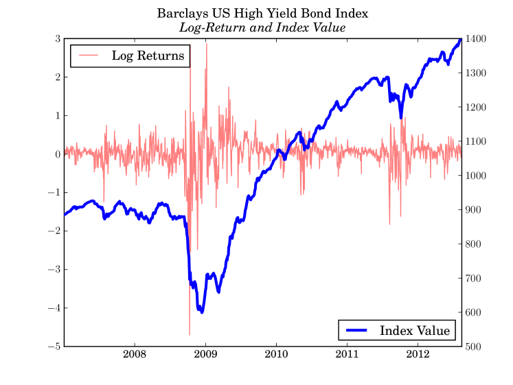
Figure 4.1: Barclays US High Yield Bond Index – Daily log-returns (in %) and index value from January 3rd, 2007 and July 31st, 2012.

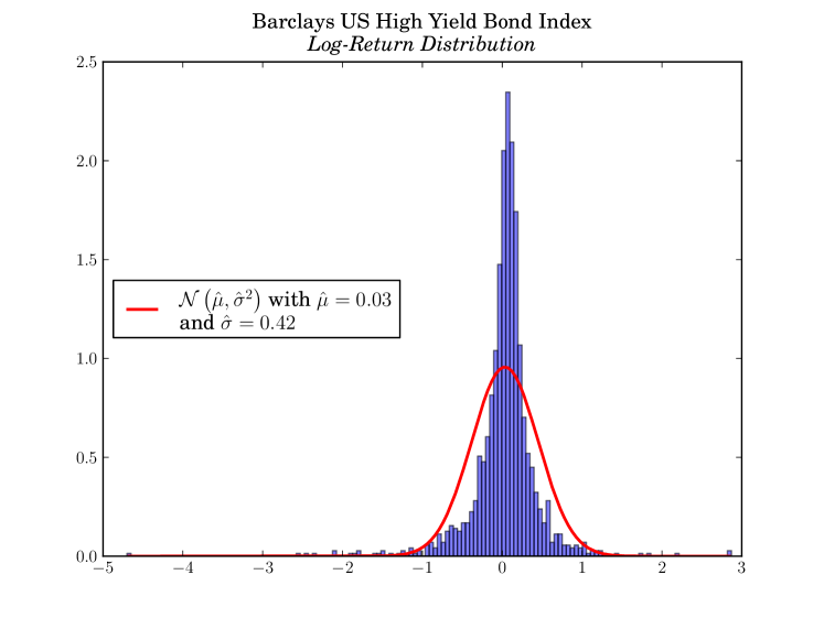
Figure 4.2: Histogram of the daily returns. The returns show negative sample skewness equal to $-1.63$ and a sample kurtosis equal to $24.08$. The sample mean $\hat{\mu}$ and standard deviation $\hat{\sigma}^{2}$ are in %.

4.1 Optimization with Differential Evolution

The main challenge that we faced from an optimization point of view is the fact the objective function (3.2) possesses several local optima. To overcome this issue, we have decided to use the optimizer described in Ardia and Mullen (2013). The main motivations for us to choose it is its easiness to use, its capacity to handle local optima and its ability to manage constraints about the parameters. Moreover, it was successfully tested in Ardia et al. (2011b) on diffusion problems. Finally, this kind of algorithm has proved to be flexible enough for us to customize it for the rolling analyses that we are dealing with in this paper. We call the variant we will describe later differential evolution algorithm with memory.

Optimization methods based on Differential Evolution (DE) is a class of search algorithms introduced by Storn and Price (1997) that belongs to the class of evolutionary algorithms. These algorithms assume no special mathematical property about the target function, like differentiability for gradient descents or quasi-Newton methods. It means that DE can handle non-continuous or very ill-conditioned optimization problems by searching a very large number of candidate solutions; we note that this number of candidate solutions can be fitted to the computational power one has at disposal. The price to pay on this lack of assumption is that optimization algorithms relying on DE are never guaranteed to converge towards an optimal solution. However, such meta-heuristics still seem to deliver good performances on continuous problems, see e.g. Price et al. (2005).

Roughly speaking, DE-based optimization algorithms exploit bio-inspired operations such as crossover, mutation and selection of candidate populations in order to optimize an objective function over several successive generations. Let $f:\mathbb{R}^{d}\longrightarrow\mathbb{R}$ denote the $d$-dimensional objective function that must be optimized. For the sake of simplicity, we assume that $f$ has to be minimized; this is not restrictive, as $f$ can easily be maximized by minimizing $-f$. The DE algorithm begins with a population of $v$ initial vectors $\bm{x}_{i}\in\mathbb{R}^{d}$, with $1\leq i\leq v$, that can either be randomly chosen or provided by the user. For a certain number of rounds, fixed in advance, one iterates then the following operations: for each vector $\bm{x}_{i}\in\mathbb{R}^{d}$, one selects at random three other vectors $\bm{x}_{a}$, $\bm{x}_{b}$ and $\bm{x}_{c}$, with $1\leq a,b,c,i\leq t$ being all distinct, as well as a random index $1\leq\rho\leq d$. Then, the successor $\bm{x}_{i}^{\prime}$ of $\bm{x}_{i}$ is computed as follows: given a crossover probability of $\pi\in[0,1]$, a differential weight $\omega\in[0,1]$ and $\bm{x_{i}}=(x_{i,1},\dots,x_{i,d})^{\mathsf{T}}$, for each $1\leq j\leq d$, one draws a number $r_{j}$ uniformly at random. If $r_{j}<\pi$, or if $j=\rho$, then one sets $x_{i,j}^{\prime}=x_{a,j}+\omega\cdot(x_{b,j}-x_{c,j})$; otherwise, $x_{i,j}^{\prime}=x_{i,j}$ keeps untouched. Once this mutation done, the resulting vector $\bm{x}^{\prime}$ is evaluated with respect to the objective function, and replaces $\bm{x}_{i}$ in the candidate population if it is better. Otherwise, $\bm{x}^{\prime}_{i}$ is rejected. For more details, we refer the reader to Price et al. (2005) and Storn and Price (1997). For practical purposes, several implementations of DE-based optimization algorithms are currently available, as illustrated by the web-based list of DE-based software for general purpose optimization maintained by Storn . In what follows, we rely on the package DEoptim, see Ardia and Mullen (2013); Mullen et al. (2011); Ardia et al. (2011a), which implements DE-based optimization in the R language and environment for statistical computing, see R Development Core Team (2008).

For the optimizer, we have used a maximum number of iterations of $250$, default values for the crossover probability of $\pi=0.5$ and for the differential weight $\omega=0.8$, as well as an initial population of $v=200$ vectors. We also have constrained the value of $\lambda$ to the interval $[0,252]$ to be compliant with the assumption $\lambda\Delta t<1$. The main challenge that we have faced for our rolling analysis is the lack of stability over time of some parameters of the objective function. This is illustrated in the upper graph of Figure 4.3, that depicts the values computed by the DE-based optimizer for $\lambda$.

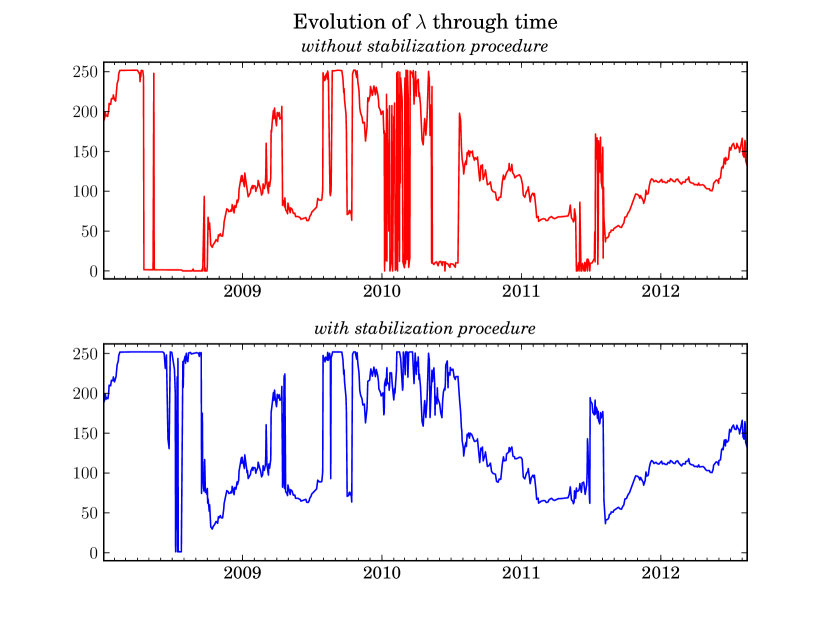
Figure 4.3: Evolution of $\lambda$ without and with the stabilization procedure. The stabilization procedure relies on feeding the initial population with the 50 last solutions, if available.

We can observe that this lack of stability can be extreme for certain periods of time. For instance, in the first half of 2010, we can see that $\lambda$ jumps from a high value near to its upper bound $252$ to a very low value the next date. This is due to the fact that objective function possesses several optima and that for each of these solutions, $\lambda$ can be very different.

In order to overcome this issue, we propose to add “memory” to the algorithm. Indeed, for each date, we compute a solution that maximizes the log-likelihood (3.2). Our idea consists in storing these solutions and to feed the initial population with the last 50 solutions of the optimization problem. Concretely, to determine the solution at a specific date, the initial population – whose size is $v=200$ – is fed with the solutions of the optimization problem at times $t-1,t-2,\ldots,t-50$. There is no reason why the solution at time $t$ is the same as time $t-1$, except if the objective function remain the same; however, it is very likely that the solution at $t-1$ will provide a good starting point for the current optimization problem if the objective function has changed, and directly an optimal solution if the objective function has not changed. With this procedure, we also have the guarantee that the solution for the date $t$ will not switch from one point to another with the same log-likelihood value at the next optimization problem of date $t+1$ if the objective function has not changed. The effect of this stabilization procedure are illustrated in the lower graph of Figure 4.3. The stabilization procedure is very important for the interpretation of our results. Without this stabilization procedure, it would be far more difficult and even impossible to interpret the results for some periods of time.

4.2 Discussion of our Results

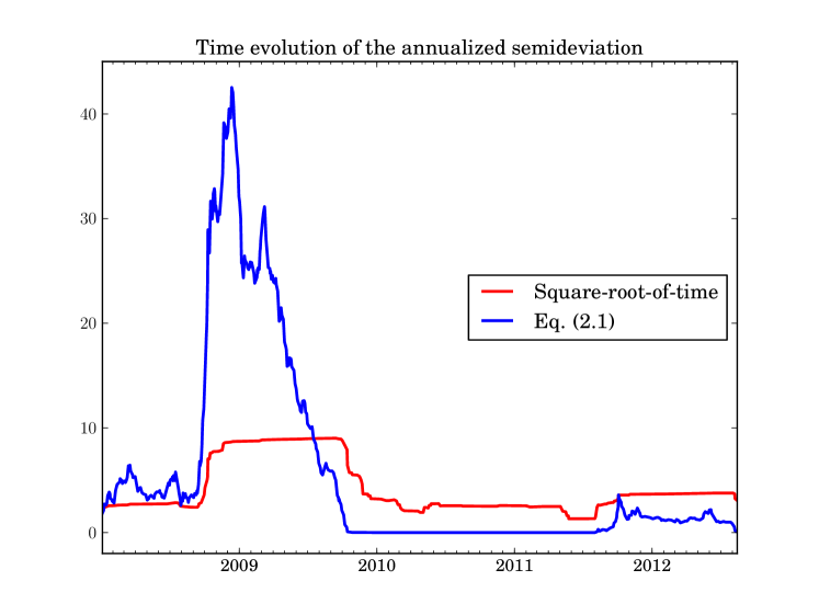
Figure 4.4: Comparison of the semideviation (in %) obtained via the square-root-of-time rule with the semideviation (in %) based on a jump-diffusion process. We can observe that the semideviation based on the square-root-of-time rule significantly underestimates the risk in periods of high volatility and overestimates the risk in periods of lower stress.

We start by comparing in Figure 4.4 the evolution of the annualized semideviation, i.e., the square root of the semivariance, computed thanks to the square-root-of-time rule to the semideviation computed through fitting a jump-diffusion process to the data under the constraint $\lambda\leq 252$ on which we applied our formula given in (3.6). It is quite striking to see that the risk estimated on the jump-diffusion process is up to 4 times larger than the one computed thanks to the square-root-of-time rule. At the beginning of 2009, the first one is larger than $40\%$ while the other is just below $10\%$. The risk is not only underestimated in period of crisis, but also seems to be overestimated when the market rallies or in period of low or medium stress. Indeed, we can observe that the jump-diffusion semideviation is almost zero from the end of 2009 to the end of 2011, while the square-root-of-time semideviation remains at a level around $2\%$ during that period.

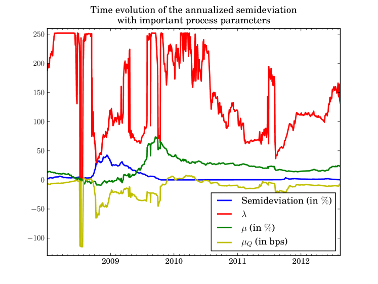
Figure 4.5: Time evolution of the jump-diffusion process parameters

4.2.1 Relationship between Important Process Parameters

To better understand how the jump-diffusion semideviation works, it is very important to understand the relationship between the different process parameters. Figure 4.5 illustrates the evolution through time of some important parameters of the jump-diffusion process, namely $\lambda$, $\mu$ and $\mu_{Q}$. We can observe a direct relationship between $\lambda$ and $\mu_{Q}$, namely that when $\lambda$ gets small, then $\mu_{Q}$ gets large (in absolute value). This behavior is quite easy to interpret: in normal market conditions, $\lambda$ is rather high, while $\mu_{Q}$ is rather low. The combination of these two parameters under normal market conditions captures a well-known effect in credit portfolios, a negative asymmetry in their return distribution.

The parameter $\mu$ has an offsetting effect counterbalancing the compound Poisson process. For example, let us assume that $\lambda=252$ and that $\mu_{Q}$ has an average size of 1 basis point. In that case, the cumulative annual impact of the accidents driven by the Poisson process is on average a negative return of $252\times 1=252$ basis points. Let us imagine that the annual return that we can expect from our investment is $7\%$, then it is very likely that the statistical estimation of $\mu$ would be around $10\%$ (note that from (1.6), we also have to take into account the role of $\sigma$ to determine the annual expected return). In crisis situation, $\lambda$ really captures the frequency of extreme events and its value typically drops from 252 to smaller values, sometimes close to 1. By contrast, $\mu$ is by construction less sensitive to these extreme accidents, even though we can see that it is impacted, by looking at Figure 4.5. Indeed, we can observe that $\mu$ has dropped to negative values during the 2008 financial crisis.

It is also quite interesting to have a look at what happened during the rally phase that started in March 2009. We can observe that $\mu$ has peaked to values larger than $60\%$. It is worth mentioning that even though the value $\mu$ has been very large at the end of 2009 due to a strong rally in the market, $\mu_{Q}$ stayed negative during that phase. It is only in year 2010 that $\mu_{Q}$ had positive values. This situation is quite exceptional, as we are used to negative skewness in the returns for credit portfolios. However, under some very particular circumstances, they can exhibit positive skewness and the values of $\mu_{Q}$ cannot be interpreted any more as losses, but as gains.

Note also that the jump-diffusion semideviation can be very close to zero in very special cases, and in particular when $\mu$ is much larger than $\lambda\cdot\mu_{Q}$, when $\mu_{Q}$ is negative or in the situation where both $\mu$ and $\mu_{Q}$ are positive. This just means that in this kind of situation, the probability of obtaining a annualized return below zero is very low, resulting in a semideviation close to zero.

The two worst crisis periods that the financial markets have experienced during the last five years are, by order of importance, the 2008 financial crisis and the US Debt Ceiling crisis in 2011. After weeks of negotiation, President Obama signed the Budget Control Act of 2011 into law on August 2, the date estimated by the department of the Treasury where the borrowing authority of the US would be exhausted. Four days later, on August 5, the credit-rating agency Standard & Poor’s downgraded the credit rating of US government bond for the first time in the country’s history. Markets around the world experienced their most volatile week since the 2008 financial crisis with the Dow Jones Industrial Average plunging for 635 points (or $5.6\%$) in a single day. However, the yields from the US Treasuries dropped as investors were more concerned by the European sovereign-debt crisis and by the economic prospect for the world economy and fled into the safety of US government bonds. This is a reason why we could see the jump-diffusion semideviation increasing substantially during that period.

4.2.2 Relationship between $\lambda$ and the Semideviation

It is worth studying the relationship between $\lambda$ and the semideviation of the jump-diffusion process. In Figure 4.6, we give the evolution of the semideviation based on different values of $\lambda$.

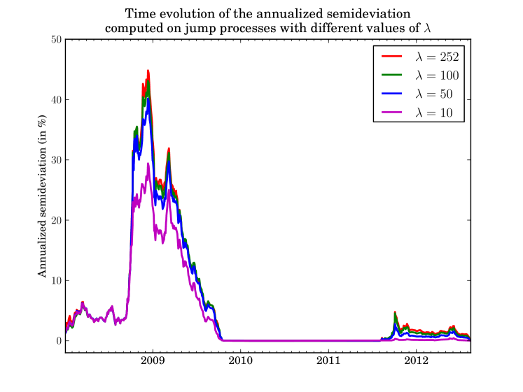
Figure 4.6: Evolution of the semideviations (in %) for different values of $\lambda$. The curve in red corresponds to the constraint $\lambda=252$, in green to $\lambda=100$, in blue to $\lambda=50$ and in violet to $\lambda=10$. Note that the curves in red and in green are almost identical.

This analysis clearly shows that the assumption made about $\lambda$ has a huge impact on the computation of the semideviation. In particular, it has been a standard practice since the publication of the work of Ball and Torous (1983) to use a Bernoulli jump diffusion process as an approximation of the true diffusion process by making the assumption that $\lambda\Delta t$ is small. However, our analysis in Figure 4.4 indicates that a model with a larger $\lambda$ fits best the data. Obviously, the motivation of Ball and Torous was to capture large and infrequent events by opposition to small and frequent jumps. However, imposing to $\lambda\Delta t$ to be small has the undesired consequence of underestimating the risk in periods of high volatility. Indeed, the graph in Figure 4.6 shows that the semideviation obtained with $\lambda=252$ can be as much as 50 % larger in a period of stress than the semideviation computed with the constraint that $\lambda=10$. This observation was the main motivation for us to extend the work of Ball and Torous by allowing models where the frequency of the jumps is not imposed anymore, but driven by the data.

In §3.2, we have shown that when $\lambda$ is large, then the jump-diffusion return distribution should be close to the distribution of a pure diffusion process but with different parameters. Rather than superposing the semideviation computed out of a jump-diffusion process with $\lambda=252$ with a pure diffusion process, we have put in Figure 4.7 the jump-diffusion semideviation and its difference with the semideviation obtained from a pure diffusion process.

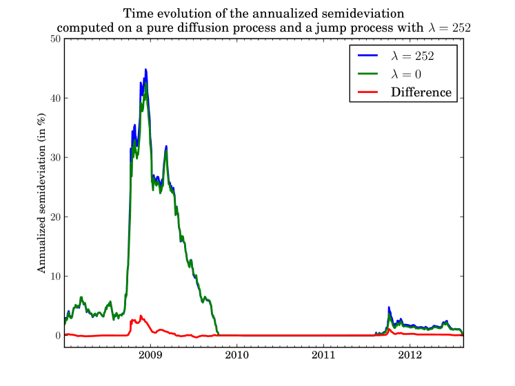
Figure 4.7: Comparison between the semideviation (in %) obtained from a jump diffusion process with $\lambda=252$ with a pure diffusion process with $\lambda=0$. The blue and green lines represent the jump-diffusion and pure diffusion semideviations, respectively, while the red one is the difference between the two. Even though the magnitude of the semideviations are similar, we can observe that the difference is substantial during the 2008 financial crisis.

The difference is small, except during the 2008 financial crisis. During that period, the difference can be larger by several %. The central limit theorem tells us that the annualized return distribution should converge to a normal distribution whose parameters are given in (3.7). But the parameters of the pure diffusion process have been determined by maximization of the log-likelihood and may give results quite different from the ones in (3.7). Moreover, we can see that the two semideviations are diverging in period of crisis, i.e., when it is difficult to calibrate the models due to the appearance of extreme events that make the determination of the parameters of the models quite challenging.

To illustrate this fact, we have depicted the evolution of the log-likelihood value for both processes on Figure 4.8. We have also compared the jump-diffusion and the Bernoulli jump-diffusion semideviations which should be the same based on the results from §3.2. Our results are displayed on Figure 4.9. The difference is negligible over all the period, meaning that our methodology provides the same results as the one based on the model of Ball and Torous provided $\lambda$ is constrained to be small.

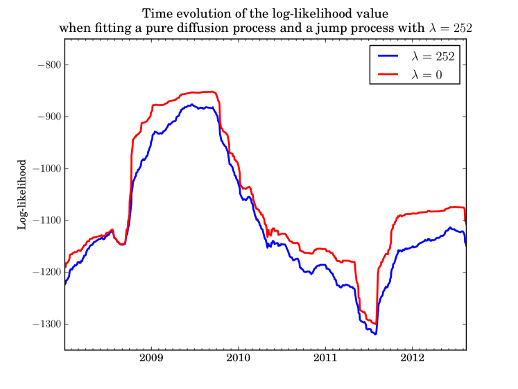
Figure 4.8: Comparison of the log-likelihood for the jump-diffusion process (in blue) with $\lambda=252$ and with the pure diffusion process (in red). In both cases, we can see that the log-likelihood is smaller in periods of high market stress, which means that the calibration of the model is also more challenging.

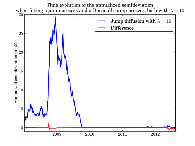
Figure 4.9: Comparison between the semideviation (in %) obtained from a jump diffusion process (in blue) and the difference with a Ball and Torous jump-diffusion (in red). In both cases, we have set $\lambda=10$. The difference is very small compared to the level of the semideviation.

4.2.3 Evolution of $\sigma$

Finally, we compare in Figure 4.10 the time evolution of the volatility $\sigma$ when fitting a jump process and a pure diffusion process. One can observe that the $\sigma$ obtained for a pure diffusion process is larger in magnitude than the one obtained for a jump diffusion process; this comes without any surprise, as in the second case, the volatility is also captured by the jumps. A second fact that we would like to outline is that $\sigma$ appears to be quite unstable for the jump process. This can be interpreted as a possible misspecification of the model, as the jumps appear to influence the value of $\sigma$. In other words, assuming a constant $\sigma$ might be a wrong hypothesis for our data, and this can be translated as a further motivation to study processes with stochastic volatility including jumps in returns and in volatility, as we will do it in the next section.

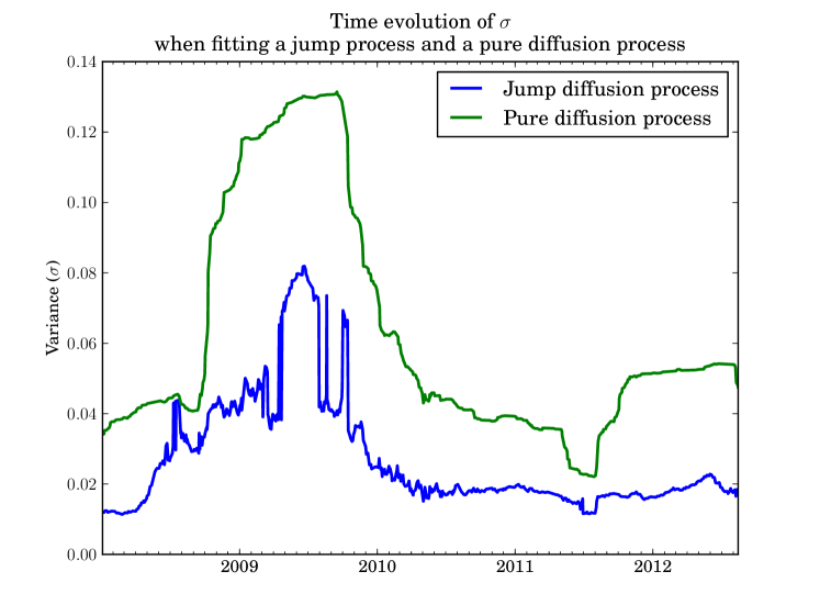
Figure 4.10: Comparison between the time evolution of the parameter $\sigma$ obtained when fitting a jump process (in blue) and a pure diffusion process (in green).

5 Extension to Stochastic Volatility Models with Jumps in Returns and Volatility

We explain now how to extend the methodology we developed before to processes involving stochastic volatility with jumps in returns and volatility. This section is structured as follows. In §5.1, we recall the importance of considering jumps in returns and in volatility. Then, in §5.2, we describe the stochastic volatility model with jumps in returns and in volatility that we consider, which is an extension of the model analyzed by  Eraker et al. (2003). The only difference is that we have replaced the Bernoulli jump process by the more general model that we have developed in §3. We continue by addressing in §5.3 the statistical estimation of the model parameters and of their posterior distributions. We have followed the approach developed in Numatsi and Rengifo (2010) and our implementation is based on a script developed in the R language provided by the same authors that we have modified in order to be able to cope with our approach. Once the parameters have been estimated, we show in §5.4 how to compute an annualized semivariance. In a nutshell, the first step consists in generating the returns over a 1-year horizon and then to compute the semivariance thanks to numerical integration. Finally, we exhibit some experimental results in §5.5.

5.1 Importance of Jumps in Returns and Volatility

Modeling accurately the price of stocks is an important topic in financial engineering. A major breakthrough was the Black and Scholes (1973) model, that however suffers from at least two major drawbacks. The first one is that the stock price follows a lognormal distribution and the second one is that its volatility is constant. Several studies (see Chernov et al. (1999), for instance) have emphasized that the asset returns’ unconditional distributions show a greater degree of kurtosis than implied by the normality assumption, and that volatility clustering is present in the data, suggesting random changes in returns’ volatility. An extension of this model is to integrate large movements in the stock prices making possible to model financial crashes, like the Black Monday (October 19th, 1987). They were introduced in the form of jump-diffusion models, see Merton (1976); Cox and Ross (1976). An important extension of the Black-Scholes model was to use stochastic volatility rather than considering it as constant, see for instance Hull and White (1987); Scott (1987); Heston (1993). Bates (1996) and Scott (1997) combined these two approaches and introduced the stochastic volatility model with jumps in returns. Event though their new approach has helped better characterize the behavior of stock prices, several studies have shown that models with both diffusive stochastic volatility and jumps in return were incapable of fully capturing the empirical features of equity index returns, see for instance Bakshi et al. (1997); Bates (2000); Pan (2002). Their main weakness is that they do not capture well the empirical fact that the conditional volatility of returns rapidly increases. By adding jumps in the volatility, then the volatility process is better specified. Duffie et al. (2000) were the first to introduce a model with jumps in both returns and volatility. Eraker et al. (2003) have shown that the new model with jumps in volatility performed better than previous ones, and resulted in no major misspecification in the volatility process.

5.2 Extension of the work of Eraker, Johannes, and Polson

As mentionned above, Eraker et al. (2003) consider a jump diffusion process with jumps in returns and in volatility. These jumps arrive simultaneously, with the jump sizes being correlated. According to the model, the logarithm of an asset’s price $Y_{t}=\log(S_{t})$ solves

(5.1) $$\left(\begin{array}[]{c}dY_{t}\\ dV_{t}\end{array}\right)=\left(\begin{array}[]{c}\mu\\ \kappa(\theta-V_{t}^{-})\end{array}\right)dt+\sqrt{V_{t^{-}}}\left(\begin{array}[]{cc}1&0\\ \rho\sigma_{\nu}&\sqrt{(1-\rho^{2})}\sigma_{\nu}\end{array}\right)d\bm{W}_{t}+\left(\begin{array}[]{c}\xi^{y}\\ \xi^{\nu}\end{array}\right)dN_{t}$$

where $V_{t}^{−}=\lim_{s\uparrow t}V_{s}$, $\bm{W}_{t}=(W_{t}^{(1)}\ W_{t}^{(2)})^{\mathsf{T}}$ is a standard Brownian motion in $\mathbb{R}^{2}$ and $(\cdot)^{\mathsf{T}}$ denotes the transpose of a matrix or a vector. The jump arrival $N_{t}$ is a Poisson process with constant intensity $\lambda$, and this model assumes that the jump arrivals for the returns and the volatility are contemporaneous. The variables $\xi^{y}$ and $\xi^{\nu}$ denote the jump sizes in returns and volatility, respectively. The jump size in volatility follows an exponential distribution $\xi^{\nu}\sim\exp(\mu_{v})$ while the jump sizes in returns and volatility are correlated with $\xi^{y}|\xi^{\nu}\sim\mathcal{N}(\mu_{y}+\rho_{j}\xi^{\nu},\sigma_{y}^{2})$.

Their methodology relies on Markov Chain Monte Carlo (MCMC) methods. The basis for their MCMC estimation is the time-discretization of (5.1):

$$Y_{t+\Delta t}-Y_{t} = \mu\Delta t+\sqrt{V_{t}\Delta t}\varepsilon_{t+\Delta t}^{y}+\xi_{t+\Delta t}^{y}J_{t+\Delta t},$$

(5.2) $$V_{t+\Delta t}-V_{t} = \kappa(\theta-V_{t})\Delta t+\sigma_{\nu}\sqrt{V_{t}\Delta t}\varepsilon_{t+\Delta t}^{\nu}+\xi_{t+\Delta t}^{\nu}J_{t+\Delta t},$$

where $J_{t+\Delta t}^{k}=1$ indicates a jump arrival. $\varepsilon_{t+\Delta t}^{y}$, $\varepsilon_{t+\Delta t}^{\nu}$ are standard normal random variables with correlation $\rho$ and $\Delta t$ is the time-discretization interval (i.e., one day). The jump sizes retain their distributional structure and the jump times are Bernoulli random variables with constant intensity $\lambda\Delta t$. The authors apply then Bayesian techniques to compute the model parameters $\bm{\Theta}$. The posterior distribution summarizes the sample information regarding the parameters $\bm{\Theta}$ as well as the latent volatility, jump times, and jump sizes:

(5.3) $$\Pr(\bm{\Theta},J,\xi^{y},\xi^{\nu},V|\bm{Y})\propto\Pr(\bm{Y}|\bm{\Theta},J,\xi^{y},\xi^{\nu},V)\Pr(\bm{\Theta},J,\xi^{y},\xi^{\nu},V)$$

where $J,\xi^{y},\xi^{\nu},V$ are vectors containing the time series of the relevant variables. The posterior combines the likelihood $\Pr(\bm{Y}|\bm{\Theta},J,\xi^{y},\xi^{\nu},V)$ and the prior $\Pr(\bm{\Theta},J,\xi^{y},\xi^{\nu},V|\bm{Y})$. As the posterior distribution is not known in closed form, the MCMC-based algorithm generates samples by iteratively drawing from the following conditional posteriors:

Parameters: $$\Pr(\bm{\Theta}_{i}|\bm{\Theta}_{-i},J,\xi^{y},\xi^{\nu},V,\bm{Y}) i=1,\dots,k$$

Jump times: $$\Pr(J_{t}=1|\bm{\Theta},\xi^{y},\xi^{\nu},V,\bm{Y}) i=1,\dots,T$$

Jump sizes: $$\Pr(\xi_{t}^{y}|\bm{\Theta},J_{t}=1,\xi^{\nu},V,\bm{Y}) i=1,\dots,T$$

$$\Pr(\xi_{t}^{\nu}|\bm{\Theta},J_{t}=1,V,\bm{Y}) i=1,\dots,T$$

Volatility: $$\Pr(V_{t}|V_{t+\Delta t},V_{t-\Delta t},\bm{\Theta},J,\xi^{y},\xi^{\nu},\bm{Y}) i=1,\dots,T$$

where $\bm{\Theta}_{-i}$ denotes the elements of the parameter vector, except $\bm{\Theta}_{i}$. Drawing from these distributions is straightforward, with the exception of the volatility, as its distribution is not of standard form. To sample from it, the authors use a random-walk Metropolis algorithm. For $\rho$, they use an independence Metropolis algorithm with a proposal density centered at the sample correlation between the Brownian increments. For a review of these MCMC techniques, we recommend Johannes and Polson (2009) where the authors provide a review of the theory behind MCMC algorithms in the context of continuous-time financial econometrics. The algorithm of Eraker et al. (2003) produces a set of draws $\left\{\bm{\Theta}^{(g)},J^{(g)},\xi^{y(g)},\xi^{\nu(g)},V^{(g)}\right\}_{g=1}^{G}$ which are samples from $\Pr(\bm{\Theta},J,\xi^{y},\xi^{\nu},V|\bm{Y})$.

Our approach relies on the methodology developed in Eraker et al. (2003). The only difference is that we have replaced the Bernoulli jump process by the jump process described in §3. This change is quite straightforward. In (5.2), $J_{t+\Delta t}$ can take only two values and its posterior is Bernoulli with parameter $\lambda\Delta t$. To compute the Bernoulli probability, the authors use the conditional independence of increments to volatility and returns to get

$$\Pr(J_{t+\Delta t}=1|V_{t+\Delta t},V_{t},Y_{t+\Delta t},\xi_{t+\Delta t}^{y},\xi_{t+\Delta t}^{\nu},\bm{\Theta})\propto$$

$$\lambda\Delta t\times\Pr(Y_{t+\Delta t},V_{t+\Delta t}|V_{t},J_{t+\Delta t}=1,\xi_{t+\Delta t}^{y},\xi_{t+\Delta t}^{\nu},\bm{\Theta}).$$

Our generalization is straightforward. Following the approach explained in §3, $J_{t+\Delta t}$ can take any value between 0 and $m$. Then

$$\Pr(J_{t+\Delta t}=m|V_{t+\Delta t},V_{t},Y_{t+\Delta t},\xi_{t+\Delta t}^{y},\xi_{t+\Delta t}^{\nu},\bm{\Theta})\propto$$

$$p_{k}\times\Pr(Y_{t+\Delta t},V_{t+\Delta t}|V_{t},J_{t+\Delta t}=m,\xi_{t+\Delta t}^{y},\xi_{t+\Delta t}^{\nu},\bm{\Theta}),$$

with $p_{k}=\frac{e^{-\lambda\Delta t}(\lambda\Delta t)^{k}}{k!}$ for $k=0,\dots,m-1$ and with $p_{m}=\sum_{k=0}^{m-1}p_{k}$.

5.3 Parameters Estimation

We have followed the approach developed by Numatsi and Rengifo (2010) for the estimation of the model parameters. These authors describe an implementation in R of the methodology exposed by Eraker et al. (2003) and apply it on FTSE 100 daily returns. We assume that we have daily data at times $t_{i}$ for $i=1,\dots,T$ and with $t_{i+1}-t_{i}=\Delta t=1\text{ day}$. The bivariate density function under consideration is given by

(5.4) $$f(\bm{B}_{t_{i}})=\frac{1}{2\pi|\bm{\Sigma}|^{0.5}}\exp\left(-\frac{1}{2}(\bm{B}_{t_{i}}-\mathrm{E}[\bm{B}_{t_{i}}])^{\mathsf{T}}\bm{\Sigma}_{t_{i}}^{-1}(\bm{B}_{t_{i}}-\mathrm{E}[\bm{B}_{t_{i}}])\right),$$

where $|\cdot|$ denotes the determinant of matrix. The likelihood function is simply given by $\prod_{i=1}^{n}f(\bm{B}_{t_{i}})$ with

(5.5) $$\bm{B}_{t_{i}}=\left(\begin{array}[]{c}\Delta y_{t_{i}}\\ \Delta\nu_{t_{i}}\end{array}\right)$$

(5.6) $$\mathrm{E}[\bm{B}_{t_{i}}]=\left(\begin{array}[]{c}\mu+\xi_{t_{i}}^{y}\xi J_{t_{i}}\\ \kappa(\theta-V_{t_{i-1}})+\xi_{t_{i}}^{\nu}J_{t_{i}}\end{array}\right)\\$$

(5.7) $$\bm{\Sigma}_{t_{i}}=\mathrm{Cov}[\Delta y_{t_{i}},\Delta\nu_{t_{i}}]=\left(\begin{array}[]{cc}V_{t_{i-1}}&\rho\sigma_{\nu}V_{t_{i-1}}\\ \rho\sigma_{\nu}V_{t_{i-1}}&\sigma_{\nu}^{2}V_{t_{i-1}}\end{array}\right)\\$$

where $\Delta y_{t_{i}}=Y_{t_{i}}-Y_{t_{i-1}}$ and $\Delta\nu_{t_{i}}=V_{t_{i}}-V_{t_{i-1}}$. The joint distribution is given by the product of the likelihood times the distributions of the state variables times the priors of the parameters, more specifically:

$$\left[\prod_{i=1}^{T}f(\bm{B}_{t_{i}})\right]\times\left[\prod_{i=1}^{T}f(\xi_{t_{i}}^{y})\times f(\xi_{t_{i}}^{\nu})\times f(J_{t_{i}})\right]$$

$$\times\left[f(\mu)\times f(\kappa)\times f(\theta)\times f(\rho)\times f(\sigma_{\nu}^{2})\times f(\mu_{y})\times f(\rho_{J})\times f(\sigma_{y}^{2})\right]$$

$$\times\left[f(\mu_{\nu})\times f(\lambda)\right]$$

The distributions of the state variables are respectively given by $\xi_{t_{i}}^{\nu}\sim\exp(\mu_{\nu})$, $\xi_{t_{i}}^{y}\sim\mathcal{N}(\mu_{y}+\rho_{J}\xi_{t_{i}}^{\nu}$, $\sigma_{y}^{2})$, and $J_{t_{i}}\sim\mathcal{B}(\lambda)$. In Numatsi and Rengifo (2010), the authors impose little information through priors, that follow the same distributions than in Eraker et al. (2003): $\mu\sim\mathcal{N}(0,1)$, $\kappa\sim\mathcal{N}(0,1)$, $\theta\sim\mathcal{N}(0,1)$, $\rho\sim\mathcal{U}(-1,1)$, $\sigma_{\nu}^{2}\sim\mathcal{IG}(2.5,0.1)$, $\mu_{y}\sim\mathcal{N}(0,100)$, $\rho_{J}\sim\mathcal{N}(0,1)$, $\sigma_{y}^{2}\sim\mathcal{IG}(5,20)$, $\mu_{\nu}\sim\mathcal{G}(20,10)$, and $\lambda\sim\beta(2,40)$. Following our approach, we only made the following change: we have relaxed the assumption about the Bernoulli process to consider the more general process proposed in §3. It may be also tempting to change the assumptions about the distribution of $\lambda$, but the $\beta$ distribution is so flexible that it can cope with a wide variety of assumptions about these parameters. For example, the $\beta(1,1)$ gives a uniform variable which can be used if we want to have a uninformative distribution.

It is important to store the sampled parameters and the vector of state variables at each iteration. The mean of each parameter over the number of iterations gives us the parameter estimate. The convergence is checked using trace plots showing the history of the chain for each parameter. ACF plots is used to analyze the correlation structure of draws. Finally, the quality of the fit may be assessed through the mean squared errors and the normal QQ plot. The standardized error is defined as follows:

$$\frac{Y_{t+\Delta t}-Y_{t}-\mu\Delta t-\xi_{t+\Delta t}^{y}J_{t+\Delta t}^{y}}{\sqrt{V_{t+\Delta t}\Delta t}}=\varepsilon_{t+\Delta t}^{y}.$$

5.4 Computing the Semideviation

Once we have managed to estimate the parameters of the model on daily data, we still have to compute an annualized semideviation. The first step consists in simulating the returns over the $\tau$ horizon, where $\tau$ is typically 1-year if we are interested in computing an annualized semideviation. We start by simulating a Poisson process $N_{\tau}$ with jump intensity $\lambda$. The output of this simulation consists of the number $N$ of jumps occurring between times 0 and $\tau$, in addition to the times $0\leq j_{1}\leq\dots\leq j_{N}\leq\tau$ at which these jumps occur. For each interval $[j_{i-1},j_{i}]$, we simulate the diffusion parts of the return and volatility processes according to an Euler discretization schema for the Heston model, this procedure being explained later in the section. This gives us preliminary values $Y_{j_{i}}^{-}$ and $V_{j_{i}}^{-}$ for the return and variance processes at time $j_{i}$. Next, we simulate jump sizes for the jumps in the two processes. These jumps are given by $\xi_{j_{i}}^{y}$ and $\xi_{j_{i}}^{\nu}$, respectively. The final values of the two processes at time $j_{i}$ can be calculated as:

(5.8) $$Y_{j_{i}} = Y_{j_{i}}^{-}+\xi_{j_{i}}^{y}$$

(5.9) $$V_{j_{i}} = V_{j_{i}}^{-}+\xi_{j_{i}}^{\nu}$$

If $j_{N}\neq\tau$, then no jump occurs in the interval $[j_{N},\tau]$, and we can apply the Euler discretization schema for the Heston model to get the values of $Y_{\tau}$ and $V_{\tau}$.

In the following, we explain how to implement the Euler discretization schema for the Heston model. Discretizing the two equations (5.1) and ignoring the jump part, the difference between $Y_{t+\Delta t}$ and $Y_{t}$ and the difference between $V_{t+\Delta t}$ and $V_{t}$ is simply given by

$$Y_{t+\Delta t}-Y_{t} = \mu\Delta t+\sqrt{V_{t}}\left(\Delta W_{t}^{(1)}\right),$$

(5.10) $$V_{t+\Delta t}-V_{t} = \kappa(\theta-V_{t})\Delta t+\sigma_{\nu}\sqrt{V_{t}}\left(\rho\Delta W_{t}^{(1)}+\sqrt{1-\rho^{2}}\Delta W_{t}^{(2)}\right).$$

As already mentioned before, we typically use $\Delta t=1$ day to discretize both processes. To simulate the Brownian increments $\Delta W_{t}^{(1)}$ and $\Delta W_{t}^{(2)}$, we use the fact that each increment is independent of the others. Each such increment is normally distributed with mean 0 and variance $\Delta t$. However, using (5.10) for the simulations may generate negative volatilities. This is a well-known effect that has been addressed several times in the literature. Following Lord et al. (2006), we slightly modify (5.10) to prevent the simulation from generating negative values:

(5.11) $$V_{t+\Delta t}-V_{t}=\kappa(\theta-V_{t}^{+})\Delta t+\sigma_{\nu}\sqrt{V_{t}^{+}}\left(\rho\Delta W_{t}^{(1)}+\sqrt{1-\rho^{2}}\Delta W_{t}^{(2)}\right),$$

where $V_{t}^{+}$ is the maximum between $0$ and $V_{t}$. If the time between different jumps is smaller that the discretization step $\Delta t$, then it simply means that we have several jumps occurring during that time interval. In that case, we just have to simulate the appropriate number of jumps, both for the return and for the volatility, during that period. In the end, the return over the period $[0,\tau]$ is just $Y_{\tau}$. By repeating this procedure $M$ times, we get $M$ realizations of the accumulated returns over the period $[0,\tau]$, which make it possible to estimate its density. In our tests, we have used a Gaussian kernel to estimate it. This can easily be done in R by using the density() function. Then, one can obtain the semivariance by numerically integrating the expression given in (1.1). For this, we have used the QUADPACK library via the use of the integrate() function in R. QUADPACK is a well known numerical analysis library implemented in FORTRAN 77 and containing very efficient methods for numerical integration of one-dimensional functions.

5.5 Results

We ran the algorithm using 100’000 iterations with 10’000 burn-in iterations. Table 5.1 provides parameter posterior means and their computed standard errors.

Parameter	Value (100k iter.)
$\mu$	0.0333 (0.0132)
$\mu_{y}$	-0.0222 (0.2055)
$\mu_{\nu}$	0.0028 (0.0007)
$\theta$	0.2087 (0.0147)
$\kappa$	0.9059 (0.0433)
$\rho$	-0.0058 (0.2595)
$\rho_{J}$	0.0050 (2.0007)
$\lambda$	0.0236 (0.0293)
$\sigma_{y}$	1.0829 (0.1379)
$\sigma_{\nu}$	0.2060 (0.0204)

Table 5.1: Estimated parameters based on 100’000 iterations. The time unit is the day rather than a year, meaning that parameters should be interpreted on a daily basis. $\mu$, $\mu_{y}$, $\mu_{\nu}$, $\sigma_{y}$, and $\sigma_{\nu}$ are in %.

The return mean $\mu$ is close to the daily return mean from the data ($0.0325\%$). The long-term mean of the $V_{t}$, given by $\mathrm{E}[V_{t}]=\theta+(\mu_{\nu}\lambda)/\kappa$, is equal to $0.2088\%$. This value is not far away from the variance of returns, which is equal to $0.1751$. The jump returns are normally distributed with mean $-0.0222\%$ and standard deviation $0.2055\%$. Concretely, it means that there is a $68\%$ likelihood of having a jump return between $-23\text{ bps}$ and $+18\text{ bps}$. The parameters $\sigma_{y}$ and $\sigma_{\nu}$ are $1.0829\%$ and $0.2060\%$, respectively. Finally, the intensity of the jumps is $0.0236$. This means that, on average, there are approximately 6 jumps per year. This is a bit low in comparison with the number of jumps that we have observed in our data, as we would rather expect an intensity around $0.05$. However, this empirical intensity was computed considering that differences in returns above $2.57$ deviations from the mean could be considered as jumps. Some caution must be taken, since this empirical intensity is very sensitive to the number of standard deviations used as threshold for defining the jumps. More details about the implementation can be found in Appendix C.

In a second step, we have computed an annualized semideviation based on that process. We have followed the methodology explained in §5.4 to first compute the simulated returns and then the semideviation.

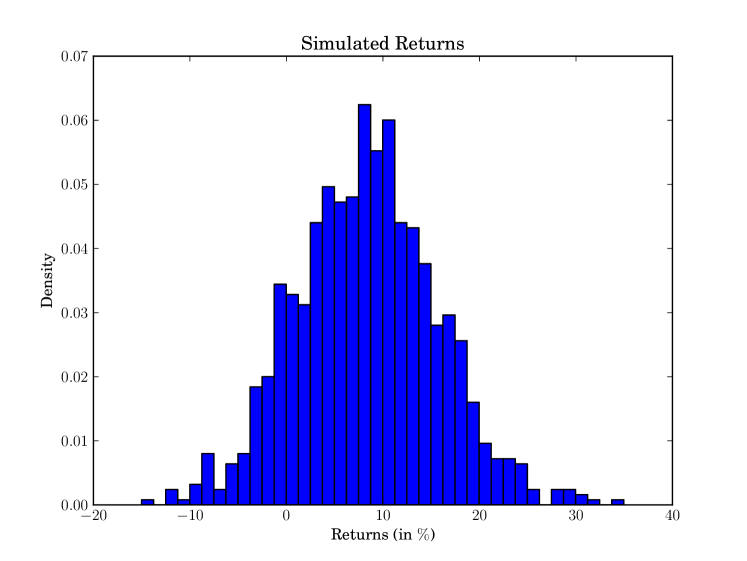
Figure 5.1: This graph shows the histogram of the returns based on 1’000 simulations.

Our tests have shown that 1’000 simulations were sufficient to get an accurate estimation of the density from which we have derived a semideviation. Note that this semideviation is based on the whole historical data. It was not possible for us to do the same rolling analysis that we have performed before, assuming a constant volatility, for the two following reasons. The first one is that the estimation of the parameters is very time-consuming. Around 7 hours were necessary to generate the parameters for the whole period with an Intel${}^{\mbox{\scriptsize{\textregistered}}}$ Core${}^{\mbox{\scriptsize{\texttrademark}}}$ i5-3470 CPU @ 3.20 GHz. Assuming that we would have to perform a rolling analysis based on 1-year of history over the same period, then we would have to run more than 1000 times this analysis. This is not impossible to realize but would typically require parallel computing techniques. The second reason for not having performed this analysis is that we have to check the convergence of the process for each period we consider in the rolling analysis, a task that is difficult to fully automate. As a reminder, the convergence can be checked with trace plots showing the history of the chain for each parameter, with ACF plots to analyze the correlation structure of draws, and the quality of the fit may be assessed through the mean squared errors and the normal QQ plot. So these two reasons have prevented us from doing this rolling analysis when we consider the model with stochastic volatility and jumps in returns and in volatility. However, we have performed some analyses based on 1 year of data for the two worst periods: during the credit crunch crisis in 2008 and in 2011. Table 5.2 summarizes the results and compares the semideviations obtained from the different models that we have explored in this paper.

Year	SD1	SD2	SD3	SD4
2008-2012	4.70	1.21	1.39	1.74
2008	8.71	31.59	31.72	32.16
2011	3.69	1.31	1.34	2.90

Table 5.2: Annualized semideviations (in %) for different periods. SD1 is based on the square-root-of-time rule, SD2 on a jump-diffusion model with constant volatility, SD3 on a pure diffusion model with a constant volatility, and SD4 is based on a jump diffusion model with stochastic volatility and jumps in returns and in volatility.

We can observe that the semideviation SD4 obtained with a stochastic volatility model seems to be more in line with the semideviations SD2 (based on a jump-diffusion model) and SD3 (based on a pure diffusion model) rather than SD1 (square-root-of-time rule). This is not very surprising since SD4 may be interpreted as a refinement of SD2, explaining why the two analytics should not be so different.

6 Conclusion and Future Venues of Research

In this paper, we propose a generalization of the Ball-Torous approximation of a jump-diffusion process and we show how to compute the semideviation based on several jump-diffusion models. We have in particular considered a very exhaustive example based on the Barclays US High Yield Index, whose returns show negative skewness and fat tails. It is a common practice to impose a bound on the Poisson process intensity parameter to make sure that only the large accidents are captured by the jumps process. However, our analysis clearly shows that the risk may be underestimated in such a situation. Without constraining the intensity parameter, the semideviation may be more than $50$ % larger than the one obtained by arbitrary limiting this parameter in order to capture only large jumps.

We see at least two reasons why our approach should be preferred. The first one is that we do not impose any arbitrary constraint on the intensity parameter. With our method, this parameter is determined in order to obtain the best fit to the data. Jumps may occur very often in certain periods and can be very uncommon (as rare as a few ones per year) in others. The second reason is that imposing an arbitrary limit on the intensity parameter may result in an underestimation of the risk. Capturing the risk as accurately as possible is one of the most important mission in risk management. It is the reason why the “traditional” approach based on the work of Ball and Torous does not seem appropriate in our context. Moreover, one of our conclusions is that the use of the square-root-of-time rule may either underestimate the risk in periods of high volatility or underestimate it in periods of lower stress.

We also provide in this paper a generalization of the work of Eraker, Johannes and Polson, who consider a jump diffusion model with stochastic volatility and jumps in returns and in volatility. As in the case where the volatility is constant, we have extended their approach by replacing the jump Bernoulli process by a more general process being able to model several accidents per day when the intensity parameter is high. The parameter estimation methods are based on MCMC methods. In particular, we have used a Gibbs sampler when the conditional distributions were known and variants of the Metropolis algorithm when it was not the case. We also provide a procedure to compute an annualized semideviation once the parameters of the model have been estimated.

It was not possible for us to go as far as we would like to when we have considered the model with stochastic volatility with jumps in returns and in volatility. It would have been very useful to be able to do the same rolling analyses that we have performed when the volatility was kept constant. However, such analyses would have been too much time consuming from a computational point of view and it would have been complicated to automate the check of the convergence of the process that needs to be done for each period in the rolling analysis. This was clearly a limitation when we have tried to determine empirically the relationship between the daily semideviation and its annualized version.

We really think that the use of the semideviation (or semivariance) could benefit the finance industry by providing a useful and powerful risk measure. This risk metric has been proposed a very long time ago but its difficulty to be computed and its lack of nice properties for its scaling made it hard to implement. However, we have shown in this article that it is still possible to calculate it even when we consider very complex stochastic processes and that some useful formula for its time scaling can be derived under some mild assumptions. Finally, we hope that this paper will help democratize its use in the asset management industry.
 
Disclaimer: The views expressed in this article are the sole responsibility of the authors and do not necessarily reflect those of Pictet Asset Management SA. Any remaining errors or shortcomings are the authors’ responsibility.

Appendix A Proof of Theorem 2.1

As a first step, we note the two following identities:

(A.1) $$\int_{-\infty}^{a}t\phi(t)\,dt=-\phi(a)\text{ and }\int_{-\infty}^{a}t^{2}\phi(t)\,dt=-a\phi(a)+\Phi(a).$$

The first one can be easily obtained by observing that $\frac{d\phi}{dt}=-t\phi(t)$ and $\lim_{t\to-\infty}\phi(t)=0$. Then,

$$\int_{-\infty}^{a}t\phi(t)\,dt=-\int_{-\infty}^{a}\frac{d}{dt}\phi(t)\,dt=\phi(a).$$

For obtaining the second identity, one can proceed as follows: we note that, for a standardized normal density $\phi$, $\int t\phi(t)\,dt=-\phi(t)$. Integrating by part, we get

$$\int_{-\infty}^{a}t^{2}\phi(t)\,dt=\int_{-\infty}^{a}t(t\phi(t))\,dt=-t\phi(t)\Bigl{|}_{-\infty}^{a}+\int_{-\infty}^{a}\phi(t)\,dt.$$

We can conclude by noting that $\lim_{t\to-\infty}t\phi(t)=0$. Those two identities are useful to prove the following result.

Proposition A.1.

Let $W\sim\mathcal{N}(\mu_{1},\sigma_{1}^{2})$, with a density function

$$f_{W}(w)=\frac{1}{\sigma_{1}\sqrt{2\pi}}\exp\left(-\frac{1}{2}\left(\frac{w-\mu_{1}}{\sigma_{1}}\right)^{2}\right),$$

and let $\tilde{D}=\frac{D-\mu_{1}}{\sigma_{1}}$; then, the semivariance of $f_{W}$ is given by

(A.2) $$\int_{-\infty}^{D}f_{W}(w)(D-w)^{2}dw=(D-\mu_{1})^{2}\Phi(\tilde{D})+\sigma_{1}(D-\mu_{1})f(\tilde{D})+\sigma_{1}^{2}\Phi(\tilde{D})$$

Proof.

By first using the change of variable $x=\frac{w-\mu_{1}}{\sigma_{1}}$ and the identities given in (A.1), we obtain the following straightforward development.

$$\int_{-\infty}^{D}f_{W}(w)(D-w)^{2}dw=\int_{-\infty}^{\tilde{D}}f(x)\left(D-(\sigma_{1}x+\mu_{1})\right)^{2}dx=$$

$$\int_{-\infty}^{\tilde{D}}(D-\mu_{1})^{2}f(x)dx+\int_{-\infty}^{\tilde{D}}2\sigma_{1}(\mu_{1}-D)xf(x)dx+\int_{-\infty}^{\tilde{D}}\sigma_{1}^{2}x^{2}f(x)dx=$$

$$(D-\mu_{1})^{2}\Phi(\tilde{D})+2\sigma_{1}(D-\mu_{1})f(\tilde{D})+\sigma_{1}^{2}\left(-\tilde{D}f(\tilde{D})+\Phi(\tilde{D})\right)=$$

$$(D-\mu_{1})^{2}\Phi(\tilde{D})+\sigma_{1}(D-\mu_{1})f(\tilde{D})+\sigma_{1}^{2}\Phi(\tilde{D})$$

∎

Taking into account that the log returns follow the density given in (1.7), we can apply Proposition A.1 on (1.7) to obtain the formula of Theorem 2.1.

Appendix B Use of a Jump-Diffusion Process to Model a Bond Benchmark Index

Using a jump-diffusion process is a standard practice for modeling a stock price. We explain here why it is possible to use this model for a bond benchmark index, because this may seem disturbing at a first sight. Indeed, the particularities of a stock and of a bond are quite different. In particular, a bond has a well-defined maturity, while it is not the case for a stock. Moreover, the clean price of a bond converges to 100 at its maturity. This is the well-known bond pull-to-par effect.

However, when considering a bond benchmark, most of criticisms in favor of not using an equity model in this context become irrelevant. Indeed, bond benchmarks have some characteristics that are quite different from a bond. For example, they are typically rebalanced on a monthly basis and their maturity are (almost) kept constant, while the maturity of a bond decreases linearly with time. The bonds with the shortest maturity (for example less than 1 year) are automatically removed from the index. A direct consequence of holding the maturity (almost) constant is that the pull-to-par effect at the portfolio level is not relevant anymore.

Another distinction between a bond and a stock is that a bond pays coupons while a stock pays dividends. When a coupon is paid, its dirty price falls for an amount equivalent to the coupons. However, it is not necessary to model the coupon payments for bond benchmarks, since the rules they obey imply that the coupons are automatically reinvested. Concretely, it means that the payment of a coupon does not impact the benchmark index.

Moreover, in a diffusion model, the stock price increases exponentially if we ignore the random part of the model. This is a direct consequence of the fact the returns are not additive, but must be compounded. This also applies to a bond benchmark index where the performance is also compounded.

Finally, as stock markets may experience crashes, bond markets may also suffered from extremely severe and sudden losses justifying the use of jumps in returns and in volatility.

All these remarks suggest that using a jump-diffusion process to model a bond benchmark index seems to be appropriate, even though the dynamics driving bonds are different from the ones driving stocks. But at the portfolio level, and when we consider a bond benchmark with a constant maturity, there is no fundamental reason for not approximating the dynamics of the index level as if it were a stock price.

Appendix C Details about the Implementation

Our MCMC algorithm is implemented in R language and relies on the code provided by Numatsi and Rengifo (2010). We have modified their implementation in order to cope with the model that we have introduced in this paper. The starting values for our algorithm were generated as follows. The volatility vector was created using a three-month rolling window. We considered as jumps absolute returns (the absolute value of the returns) that were above $2.57$ standard deviations above the mean (after accounting for outliers). For a standardized normal distribution, $2.57$ corresponds to its $0.995$-quantile, meaning that we should expect that approximately $1\%$ of the absolute returns to be larger that this threshold. Indeed, in our data, we had more than $14\%$ of the data exceeding this threshold, confirming the presence of jumps in returns. Once these “accidents” have been identified, we still need to determine the jump return size, the jump volatility size and the number of jumps that have happened. Indeed, with our methodology, it is possible to have more than a single jump occurring during a specific date. Provided that the jump sizes are by construction far larger than that returns observed during the days without “accidents”, we have considered that the jump size corresponds to the observed daily returns. For example, if we have identified a jump and if the observed return is -67 bps for that date, then we consider that the jump size is the same amount. We have made a similar assumption for the volatility. So the volatility jump simply correspond to the difference in volatility between the actual estimation for a particular day and the day before. The process followed by the sum of the jump returns is a Poisson compound variable with normally distributed jumps. The same for the process followed by the sum of the volatility jumps, except that the jumps are this time exponentially distributed. Provided that the jumps can be negative or positive for returns but not for the volatilities (always positive), it is much easier to consider the volatility to determine the number of jumps. It is the reason why we consider a compound Poisson process $X$ for the jumps in volatility where the Poisson process results in a $\mathcal{P}(\lambda)$ and the jump sizes are exponential variables $\xi^{\nu}$ of parameter $\nu$. It is easy to show that the distribution function $F(x)$ of the process $X$ is simply given by

$$F(x)=\Pr(X\leq x)=\sum_{k=0}^{+\infty}p_{k}\Pr\left(\sum_{i=1}^{k}\xi^{\nu}\right),$$

where $p_{k}=e^{-\lambda}\frac{\lambda^{k}}{k!}$. If there is no jump, then $X=0$ with probability $p_{0}=e^{-\lambda}$. A direct consequence is that the density does not exist. In order to overcome this issue, we propose to estimate $\lambda$ based on the proportion of days having at least a jump. The probability of having no accident in a particular day is $e^{-\lambda}\approx 1-\lambda$, when $\lambda$ is small. From that formula, we can simply estimate $\lambda$ by the ratio of days with at least one jump over the total number of days within that period.

Once these parameters have been estimated, we still need to determine the number of jumps occurring when an accident is detected. It is well-known that the convolution of $k$ iid exponential variables is given by a Gamma distribution with parameters $k$ and $\lambda$. So, based on the observation of the jump size, we can determine the number of jumps by determining which $k$ gives the highest density.

Having determined the state space variables, we can now tackle the problem of estimating the model parameters. We have implemented either the Gibbs sampler or Metropolis-Hasting depending on whether or not we knew the closed form of the parameters’ distributions. In order to able to compare our results with those in Eraker et al. (2003) and in Numatsi and Rengifo (2010), we have used the same priors. Note that little information is imposed through priors. They are as follows: $\mu\sim\mathcal{N}(0,1),\kappa\sim\mathcal{N}(0,1),\kappa\theta\sim\mathcal{N}(0,1),\rho\sim\mathcal{U}(-1,1),\sigma_{\nu}^{2}\sim\mathcal{IG}(2.5,0.1),\mu_{y}\sim\mathcal{N}(0,100),\rho_{J}\sim\mathcal{N}(0,1),\sigma_{y}^{2}\sim\mathcal{IG}(5,20),\mu_{\nu}\sim\mathcal{G}(20,10)$, and $\lambda\sim\beta(2,40)$. Another reason for us to use parameters provided by other studies is to guarantee that the priors have been determined independently from their posterior distributions. In Eraker et al. (2003), it was also shown that these priors may lead to very different posteriors when applied to S&P 500 and Nasdaq 100 index returns. Moreover, the main objective of our work is not to challenge the estimation of the parameters and in particular the assumptions about the priors, but merely to show that it is possible to compute a semideviation even when we consider complex stochastic processes.

References

- Ardia et al. (2011a) Ardia, D., Boudt, K., Carl, P., Mullen, K. M., and Peterson, B. G. (2011a). Differential evolution with DEoptim – an application to non-convex portfolio optimization. The R Journal, 3(1):27–34.
- Ardia et al. (2011b) Ardia, D., David, J., Arango, O., and Gómez, N. D. G. (2011b). Jump-diffusion calibration using differential evolution. Willmott, 2011(55):76–79.
- Ardia and Mullen (2013) Ardia, D. and Mullen, K. M. (2013). DEoptim: Differential evolution optimization in R, version 2.2-2. http://CRAN.R-project.org/package=DEoptim.
- Bakshi et al. (1997) Bakshi, G., Cao, C., and Chen, Z. (1997). Empirical performance of alternative option pricing models. Journal of Finance, 52:2003 – 2049.
- Ball and Torous (1983) Ball, C. A. and Torous, W. N. (1983). A simplified jump process for common stock returns. Journal of Financial and Quantitative Analysis, 18:53–65.
- Ball and Torous (1985) Ball, C. A. and Torous, W. N. (1985). On jumps in common stock prices and their impact on call option pricing. The Journal of Finance, 40(1):155–173.
- Bates (1996) Bates, D. (1996). Jumps and stochastic volatility: the exchange rate processes implicit in deutschemark options. Review of Financial Studies, 9:69–107.
- Bates (2000) Bates, D. (2000). Post 87 crash fears in SP 500 futures options. Journal of Econometrics, 94:181–238.
- Bawa (1975) Bawa, V. S. (1975). Optimal rules for ordering uncertain prospects. Journal of Financial Economics, 2(1):95–121.
- Beckers (1981) Beckers, S. (1981). A note on estimating the parameters of the jump-diffusion model of stock returns. Journal of Financial and Quantitative Analysis, 16.
- Black and Scholes (1973) Black, F. and Scholes, M. (1973). The pricing of options and corporate liabilities. The Journal of Political Economy, pages 637–654.
- Chernov et al. (1999) Chernov, M., Gallant, A. R., Ghysels, E., and Tauchen, G. (1999). A new class of stochastic volatility models with jumps: Theory and estimation. SSRN eLibrary.
- Cont and Tankov (2004) Cont, R. and Tankov, P. (2004). Financial Modelling with Jump Processes. Chapman & Hall.
- Cox and Ross (1976) Cox, J. C. and Ross, S. A. (1976). The valuation of options for alternative stochastic processes. Journal of Financial Economics, 3:145–166.
- Daníelsson and Zigrand (2006) Daníelsson, J. and Zigrand, J.-P. (2006). On time-scaling of risk and the square-root-of-time rule. Journal of Banking & Finance, 30(10):2701–2713.
- Duffie et al. (2000) Duffie, D., Pan, J., and Singleton, K. J. (2000). Transform analysis and asset pricing for affine jump-diffusions. Econometrica, pages 1343–1376.
- Eraker et al. (2003) Eraker, B., Johannes, M., and Polson, N. (2003). The impact of jumps in volatility and returns. The Journal of Finance, 58(3):1269–1300.
- Fishburn (1977) Fishburn, P. C. (1977). Mean-risk analysis with risk associated with below-target returns. American Economic Review, 67(2):116–126.
- Heston (1993) Heston, S. (1993). A closed-form solution for options with stochastic volatility with applications to bond and currency options. The Review of Financial Studies, 6:1993.
- Honore (1998) Honore, P. (1998). Pitfalls in estimating jump-diffusion models. Working Paper
- Hull and White (1987) Hull, J. C. and White, A. (1987). The pricing of options on assets with stochastic volatilities. Journal of Finance, 42:281–300.
- Johannes and Polson (2009) Johannes, M. and Polson, N. (2009). Handbook of Financial Econometrics, volume 2, chapter MCMC Methods for Continuous-Time Financial Econometrics. Elsevier Science.
- Kiefer (1978) Kiefer, N. (1978). Discrete parameter variation: Efficient estimation in diffusion process. Econometrica, 2:427–434.
- Lord et al. (2006) Lord, R., Koekkoek, R., and van Dijk, D. (2006). A comparison of biased simulation schemes for stochastic volatility models. Technical report, University Rotterdam, Rabobank International and Robeco Alternative Investments.
- Markowitz (1952) Markowitz, H. M. (1952). Portfolio selection. Journal of Finance, 7(1):77–91.
- Markowitz (1959) Markowitz, H. M. (1959). Portfolio selection. John Wiley and Sons.
- Merton (1976) Merton, R. C. (1976). Option pricing when underlying stock returns are discontinuous. Journal of Financial Economics, pages 125–144.
- Mullen et al. (2011) Mullen, K. M., Ardia, D., Gil, D. L., Windover, D., and Cline, J. (2011). DEoptim: An R package for global optimization by differential evoluation. Journal of Statistical Software, 40(6).
- Numatsi and Rengifo (2010) Numatsi, A. and Rengifo, E. (2010). Stochastic volatility model with jumps in returns and volatility: An R-package implementation. In Vinod, H., editor, Advances in Social Science Research Using R. Springer Science+Business Media.
- Pan (2002) Pan, J. (2002). The jump-risk premia implicit in options: Evidence from an integrated time-series study. Journal of Financial Economics, pages 3–50.
- Price et al. (2005) Price, K., Storn, R. M., and Lampinen, J. A. (2005). Differential evolution – a practical approach to global optimization. Natural Computing Series. Springer-Verlag.
- R Development Core Team (2008) R Development Core Team (2008). R: A Language and Environment for Statistical Computing. R Foundation for Statistical Computing, Vienna, Austria. http://www.R-project.org.
- Roy (1952) Roy, A. D. (1952). Safety first and the holding of assets. Econometrica, 20(3):431–449.
- Scott (1997) Scott, L. (1997). Pricing stock options in a jump-diffusion model with stochastic volatility and interest rates: Applications of Fourier inversion methods. Mathematical Finance, 7:413–426.
- Scott (1987) Scott, L. O. (1987). Option pricing when the variance changes randomly: Theory, estimation, and an application. Journal of Financial and Quantitative Analysis, 22:419–438.
- Sharpe (1966) Sharpe, W. F. (1966). Mutual fund performance. Journal of Business, 39(1):119–138. Part II.
- Sortino and Van Der Meer (1991) Sortino, F. A. and Van Der Meer, R. (1991). Downside risk. Journal of Portfolio Management, 17(4):27–32.
- Storn and Price (1997) Storn, R. and Price, K. (1997). Differential evolution – a simple and efficient heuristic for global optimization over continuous spaces. Journal of Global Optimization, 11(4):341–359.
- (39) Storn, R. M. Differential evolution for continuous function optimization. http://www.icsi.berkeley.edu/~storn/code.html.