Mirror Prox Algorithm for Multi-Term Composite Minimization and Semi-Separable Problems
Abstract
In the paper, we develop a composite version of Mirror Prox algorithm for solving convex-concave saddle point problems and monotone variational inequalities of special structure, allowing to cover saddle point/variational analogies of what is usually called “composite minimization” (minimizing a sum of an easy-to-handle nonsmooth and a general-type smooth convex functions “as if” there were no nonsmooth component at all). We demonstrate that the composite Mirror Prox inherits the favourable (and unimprovable already in the large-scale bilinear saddle point case) efficiency estimate of its prototype. We demonstrate that the proposed approach can be successfully applied to Lasso-type problems with several penalizing terms (e.g. acting together and nuclear norm regularization) and to problems of semi-separable structures considered in the alternating directions methods, implying in both cases methods with the complexity bounds.
Keywords:
numerical algorithms for variational problems, composite optimization, minimization problems with multi-term penalty, proximal methods
MSC(AMS):
65K10, 65K05, 90C06, 90C25, 90C47.
1 Introduction
1.1 Motivation
Our work is inspired by the recent trend of seeking efficient ways for solving problems with hybrid regularizations or mixed penalty functions in fields such as machine learning, image restoration, signal processing and many others. We are about to present two instructive examples (for motivations, see, e.g., [6, 2, 7]).
Example 1. (Matrix completion)
Our first motivating example is matrix completion problem, where we want to reconstruct the original matrix , known to be both sparse and low-rank, given noisy observations of part of the entries. Specifically, our observation is , where is a given set of cells in an matrix, is the restriction of onto , and is a random noise. A natural way to recover from is to solve the optimization problem
| (1) |
where are regularization parameters. Here is the Frobenius norm, is the -norm, and ( are the singular values of ) is the nuclear norm of a matrix .
Example 2. (Image recovery)
Our second motivating example is image recovery problem, where we want to recover an image from its noisy observations , where is a given affine mapping (e.g. the restriction operator defined as above, or some blur operator), and is a random noise. Assume that the image can be decomposed as where is of low rank, is the matrix of contamination by a “smooth background signal”, and is a sparse matrix of “singular corruption.” Under this assumption in order to recover from it is natural to solve the optimization problem
| (2) |
where are regularization parameters. Here is the total variation of an image :
These and other examples motivate addressing the following multi-term composite minimization problem
| (3) |
and, more generally, the semi-separable problem
| (4) |
Here for the domains are closed and convex, are convex Lipschitz-continuous functions, and are convex functions which are “simple and fit” .111The precise meaning of simplicity and fitting will be specified later. As of now, it suffices to give a couple of examples. When is the norm, can be the entire space, or the centered at the origin -ball, ; when is the nuclear norm, can be the entire space, or the centered at the origin Frobenius/nuclear norm ball.
The problem of multi-term composite minimization (3) has been considered (in a somewhat different setting) in [21] for . When , problem (3) becomes the usual composite minimization problem:
| (5) |
which is well studied in the case where is a smooth convex function and is a simple non-smooth function. For instance, it was shown that the composite versions of Fast Gradient Method originating in Nesterov’s seminal work [20] and further developed by many authors (see, e.g., [3, 4, 8, 26, 24] and references therein), as applied to (5), work as if there were no nonsmooth term at all and exhibit the convergence rate, which is the optimal rate attainable by first order algorithms of large-scale smooth convex optimization. Note that these algorithms cannot be directly applied to problems (3) with .
The problem with semi-separable structures (4) for , has also been extensively studied using the augmented Lagrangian approach (see, e.g., [25, 5, 23, 27, 11, 12, 16, 22] and references therein). In particular, much work was carried out on the alternating directions method of multipliers (ADMM, see [5] for an overview), which optimizes the augmented Lagrangian in an alternating fashion and exhibits an overall convergence rate. Note that the available accuracy bounds for those algorithms involve optimal values of Lagrange multipliers of the equality constraints (cf. [22]). Several variants of this method have been developed recently to adjust to the case for (see, e.g.[10]), however, most of these algorithms require to solve iteratively subproblems of type (5) especially with the presence of non-smooth terms in the objective.
1.2 Our contribution
In this paper we do not assume smoothness of functions , but, instead, we suppose that are saddle point representable:
| (6) |
where are smooth functions which are convex-concave (i.e., convex in their first and concave in the second argument), are convex and compact, and are simple convex functions on . Let us consider, for instance, the multi-term composite minimization problem (3). Under (6), the primal problem (3) allows for the saddle point reformulation:
| (7) |
Note that when there are no ’s, problem (7) becomes a convex-concave saddle point problem with smooth cost function, studied in [14]. In particular, it was shown in [14] that Mirror Prox algorithm originating from [17], when applied to the saddle point problem (7), exhibits the “theoretically optimal” convergence rate . Our goal in this paper is to develop novel -converging first order algorithms for problem (7) (and also the related saddle point reformulation of the problem in (4)), which appears to be the best rate known, under circumstances, from the literature (and established there in essentially less general setting than the one considered below).
Our key observation is that composite problem (3), (6) can be reformulated as a smooth linearly constrained saddle point problem by simply moving the nonsmooth terms into the problem domain. Namely, problem (3) , (6) can be written as
We can further approximate the resulting problem by penalizing the equality constraints, thus passing to
| (8) |
where are penalty parameters and .
We solve the convex-concave saddle point problem (8) with smooth cost function by -converging Mirror Prox algorithm. It is worth to mention that if the functions , are Lipschitz continuous on the domains , and are selected properly, the saddle point problem is exactly equivalent to the problem of interest.
The monotone operator associated with the saddle point problem in (8) has a special structure: the variables can be split into two blocks (all -, - and -variables) and (all - and -variables) in such a way that the induced partition of is with the -component depending solely on and constant -component . We demonstrate below that in this case the basic Mirror Prox algorithm admits a “composite” version which works essentially “as if” there were no -component at all. This composite version of Mirror Prox will be the working horse of all subsequent developments.
The main body of this paper is organized as follows. In section 2 we present required background on variational inequalities with monotone operators and convex-concave saddle points. In section 3 we present and justify the composite Mirror Prox algorithm. In sections 4 and 5, we apply our approach to problems (3), (6) and (4), (6). In section 4.4, we illustrate our approach (including numerical results) as applied to the motivating examples. All proofs missing in the main body of the paper are relegated to the appendix.
2 Preliminaries: Variational Inequalities and Accuracy Certificates
Execution protocols and accuracy certificates.
Let be a nonempty closed convex set in a Euclidean space and be a vector field.
Suppose that we process by an algorithm which generates
a sequence of search points , , and computes the vectors , so that after steps we have at our disposal -step execution protocol
. By definition, an accuracy certificate for this protocol is simply a collection of nonnegative reals summing up to 1.
We associate with the protocol and accuracy certificate two quantities as follows:
-
•
Approximate solution , which is a point of ;
-
•
Resolution on a subset of given by
(9)
The role of those notions in the optimization context is explained next222our exposition follows [18]..
Variational inequalities.
Assume that is monotone, i.e.,
| (10) |
and let our goal be to approximate a weak solution to the variational inequality (v.i.) associated with ; weak solution is defined as a point such that
| (11) |
A natural (in)accuracy measure of a candidate weak solution to is the dual gap function
| (12) |
This inaccuracy is a convex nonnegative function which vanishes exactly at the set of weak solutions to the vi .
Proposition 2.1
For every , every execution protocol and every accuracy certificate one has . Besides this, assuming monotone, for every closed convex set such that one has
| (13) |
Proof. Indeed, is a convex combination of the points with coefficients , whence . With as in the premise of Proposition, we have
where the first is due to monotonicity of .
Convex-concave saddle point problems.
Now let , where is a closed convex subset in Euclidean space , , and , and let be a locally Lipschitz continuous function which is convex in and concave in . give rise to the saddle point problem
| (14) |
two induced convex optimization problems
| (15) |
and a vector field specified (in general, non-uniquely) by the relations
It is well known that is monotone on , and that weak solutions to the vi are exactly the saddle points of on . These saddle points exist if and only if and are solvable with equal optimal values, in which case the saddle points are exactly the pairs comprised by optimal solutions to and . In general, , with equality definitely taking place when at least one of the sets is bounded; if both are bounded, saddle points do exist. To avoid unnecessary complications, from now on, when speaking about a convex-concave saddle point problem, we assume that the problem is proper, meaning that and are reals; this definitely is the case when is bounded.
A natural (in)accuracy measure for a candidate to the role of a saddle point of is the quantity
| (16) |
This inaccuracy is nonnegative and is the sum of the duality gap (always nonnegative and vanishing when one of the sets is bounded) and the inaccuracies, in terms of respective objectives, of as a candidate solution to and as a candidate solution to .
The role of accuracy certificates in convex-concave saddle point problems stems from the following observation:
Proposition 2.2
Let be nonempty closed convex sets, be a locally Lipschitz continuous convex-concave function, and be the associated monotone vector field on .
Let be a -step execution protocol associated with and be an associated accuracy certificate. Then .
Assume, further, that and are closed convex sets such that
| (17) |
Then
| (18) |
In addition, setting , for every we have
| (19) |
In particular, when the problem is solvable with an optimal solution , we have
| (20) |
3 Composite Mirror Prox Algorithm
3.1 The situation
Let be a nonempty closed convex domain in a Euclidean space , be a Euclidean space, and be a nonempty closed convex domain in . We denote vectors from by with blocks belonging to and , respectively.
We assume that
-
A1:
is equipped with a norm , the conjugate norm being , and is equipped with a distance-generating function (d.g.f.) (that is, with a continuously differentiable convex function ) which is compatible with , meaning that is strongly convex, modulus 1, w.r.t. .
Note that d.g.f. defines the Bregman distance
(22) where the concluding inequality follows from strong convexity, modulus 1, of the d.g.f. w.r.t. .
In the sequel, we refer to the pair as to proximal setup for .
-
A2:
the image of under the projection is contained in .
-
A3:
we are given a vector field on of the special structure as follows:
with and . Note that is independent of .
We assume also that
(23) with some , .
-
A4:
the linear form of is bounded from below on and is coercive on w.r.t. : whenever , is a sequence such that is bounded and as , we have , .
Our goal
in this section is to show that in the situation in question, proximal type processing (say, is monotone on , and we want to solve the variational inequality given by and ) can be implemented “as if” there were no -components in the domain and in .
A generic application we are aiming at is as follows. We want to solve a “composite” saddle point problem
| (24) |
where
-
•
and are nonempty closed convex sets in Euclidean spaces
-
•
is a smooth (with Lipschitz continuous gradient) convex-concave function on
-
•
and are convex functions, perhaps nonsmooth, but “fitting” the domains , in the following sense: for , we can equip with a norm , and - with a compatible with this norm d.g.f. in such a way that optimization problems of the form
(25) are easy to solve.
Our ultimate goal is to solve (24) “as if” there were no (perhaps) nonsmooth terms . With our approach, we intend to “get rid” of the nonsmooth terms by “moving” them into the description of problem’s domains. To this end, we act as follows:
-
•
For , we set and set
thus ensuring that , where ;
-
•
We rewrite the problem of interest equivalently as
(26) Note that is convex-concave and smooth. The associated monotone operator is
and is of the structure required in A3. Note that is Lipschitz continuous, so that (23) is satisfied with properly selected and with .
We intend to process the reformulated saddle point problem (26) with a properly modified state-of-the-art Mirror Prox (MP) saddle point algorithm [17]. In its basic version and as applied to a variational inequality with Lipschitz continuous monotone operator (in particular, to a convex-concave saddle point problem with smooth cost function), this algorithm exhibits rate of convergence, which is the best rate achievable with First Order saddle point algorithms as applied to large-scale saddle point problems (even those with bilinear cost function). The basic MP would require to equip the domain of (26) with a d.g.f. resulting in an easy-to-solve auxiliary problems of the form
| (27) |
which would require to “account nonlinearly” for the -variables (since should be a strongly convex in both - and -variables). While it is easy to construct from our postulated “building blocks” , leading to easy-to-solve problems (25), this construction results in auxiliary problems (27) somehow more complicated than problems (25). To overcome this difficulty, below we develop a “composite” Mirror Prox algorithm taking advantage of the special structure of , as expressed in A3, and preserving the favorable efficiency estimates of the prototype. The modified MP operates with the auxiliary problems of the form
that is, with pairs of uncoupled problems
recalling that , these problems are nothing but the easy-to-solve problems (25).
3.2 Composite Mirror-Prox algorithm
Given the situation described in section 3.1, we define the associated prox-mapping: for and ,
| (28) |
Observe that is well defined whenever – the required is nonempty due to the strong convexity of on and assumption A4 (for verification, see item 0o in Appendix A). Now consider the process as follows:
| (29) |
where ; the latter relation, due to the above, implies that the recurrence (29) is well defined.
Theorem 3.1
In the setting of section 3.1, assuming that A1–A4 hold, consider the Composite Mirror Prox recurrence (29) (CoMP) with stepsizes , satisfying the relation:
| (30) |
Then the corresponding execution protocol admits accuracy certificate such that for every it holds
| (31) |
Relation (30) is definitely satisfied when , or, in the case of , when .
Corollary 3.1
Under the premise of Theorem 3.1, for every , setting
we ensure that and that
(i) In the case when is monotone on , we have
| (32) |
(ii) Let , and let be the monotone vector field associated with the saddle point problem (14) with convex-concave locally Lipschitz continuous cost function . Then
| (33) |
In addition, assuming that problem in (15) is solvable with optimal solution and denoting by the projection of onto , we have
| (34) |
Remark 3.1
When is Lipschitz continuous (that is, (23) holds true with some and ), the requirements on the stepsizes imposed in the premise of Theorem 3.1 reduce to for all and are definitely satisfied with the constant stepsizes . Thus, in the case under consideration we can assume w.l.o.g. that , thus ensuring that the upper bound on in (31) is . As a result, (34) becomes
| (35) |
3.3 Modifications
In this section, we demonstrate that in fact our algorithm admits some freedom in building approximate solutions, freedom which can be used to improve to some extent solutions’ quality. Modifications to be presented originate from [19]. We assume that we are in the situation described in section 3.1, and assumptions A1 – A4 are in force. In addition, we assume that
-
A5:
The vector field described in A3 is monotone, and the variational inequality given by has a weak solution:
(36)
Lemma 3.1
In the situation from section 3.1 and under assumptions A1 – A5, for let us set
| (37) |
(this quantity is finite since is continuously differentiable on ), and let
be the trajectory of the -step Mirror Prox algorithm (29) with stepsizes which ensure (30) for . Then for all and ,
| (38) |
with defined in (36).
Proposition 3.1
In the situation of section 3.1 and under assumptions A1 – A5, let be a positive integer, and let be the execution protocol generated by -step Composite Mirror Prox recurrence (29) with stepsizes ensuring (30). Let also be a collection of positive reals summing up to 1 and such that
| (39) |
Then for every , with one has
| (40) |
Corollary 3.2
Under the premise and in the notation of Proposition 3.1, setting
we ensure that . Besides this,
(i) Let be a closed convex subset of such that and the projection of on the -space is contained in -ball of radius centered at . Then
| (41) |
(ii) Let and be the monotone vector field associated with saddle point problem (14) with convex-concave locally Lipschitz continuous cost function . Let, further, be closed convex subsets of , , such that and the projection of onto the -space is contained in -ball of radius centered at . Then
| (42) |
4 Multi-Term Composite Minimization
4.1 Problem setting
We intend to consider problem (3), (6) in the situation as follows. For a nonnegative integer and we are given
-
1.
Euclidean spaces and along with their nonempty closed convex subsets and , respectively;
-
2.
Proximal setups for and , that is, norms on , norms on , and d.g.f.’s , compatible with and , respectively;
-
3.
Affine mappings , where is the identity mapping on ;
-
4.
Lipschitz continuous convex functions along with their saddle point representations
(43) where are smooth (with Lipschitz continuous gradients) functions convex in and concave in , and are Lipschitz continuous convex functions such that the problems of the form
(44) are easy to solve;
-
5.
Lipschitz continuous convex functions such that the problems of the form
(45) are easy to solve;
-
6.
For , the norms on are given, with conjugate norms , along with d.g.f.’s which are strongly convex, modulus 1, w.r.t. such that the problems
(46) are easy to solve.
The outlined data define the sets
The problem of interest
(3), (6) along with its saddle point reformulation in the just defined situation read
| Opt | (47a) | |||
| (47b) | ||||
| which we rewrite equivalently as | ||||
| (47c) | ||||
From now on we make the following assumptions
B1: We have , ;
B2: For , the sets are bounded. Further, the functions are below bounded on , and the functions are coercive on : whenever , , are such that as , we have .
Note that B1 and B2 imply that the saddle point problem (47c) is solvable; let be the corresponding saddle point.
4.2 Course of actions
Given , , we approximate (47c) by the problem
| (48a) | ||||
| (48b) | ||||
where
Observe that the monotone operator associated with the saddle point problem in (48b) is given by
| (49) |
Now let us set
-
•
-
•
,
so that , cf. assumption A2 in section 3.1.
The variational inequality associated with the saddle point problem in (48b) can be treated as the variational inequality on the domain with the monotone operator
where
| (50) |
This operator meets the structural assumptions A3 and A4 from section 3.1 (A4 is guaranteed by B2). We can equip and its embedding space with the proximal setup given by
| (51) |
where , , and , , are positive aggregation parameters. Observe that carrying out a step of the CoMP algorithm presented in section 3.2 requires computing at points of and solving auxiliary problems of the form
with positive , and we have assumed that these problems are easy to solve.
4.3 “Exact penalty”
Let us make one more assumption:
C: For ,
- •
are Lipschitz continuous on with constants w.r.t. ,
- •
are Lipschitz continuous on with constants w.r.t. .
Given a feasible solution , to the saddle point problem (48b), let us set
thus getting another feasible (by assumption B1) solution to (48b). We call correction of . For we clearly have
and . Hence for we have
We see that under the condition
| (52) |
correction does not increase the value of the primal objective of (48b), whence the saddle point value of (48b) is the optimal value Opt in the problem of interest (47a). Since the opposite inequality is evident, we arrive at the following
Proposition 4.1
- (i)
- (ii)
As a corollary, under the premise of Proposition 4.1, when applying to the saddle point problem (48b) the CoMP algorithm induced by the above setup and passing “at no cost” from the approximate solutions generated by CoMP to the corrections of ’s, we get feasible solutions to the problem of interest (47a) satisfying the error bound
| (54) |
where is the Lipschitz constant of induced by the norm given by (51), and is induced by the d.g.f. given by the same (51) and the -component of the starting point. Note that and are compact, whence is finite.
Remark.
Note that the value of the penalty in (52) which guarantees the validity of correction (the bound (53) of Proposition 4.1) may be very conservative. When implementing the algorithm the coefficients of penalization can be adjusted on-line. Indeed, let (cf (15)). We always have . It follows that independently of how are selected, we have
| (55) |
for every feasible solution to (48b) and the same inequality holds for its correction . When is a component of a good (with small ) approximate solution to the saddle point problem (48b), is small. If also is small, we are done; otherwise we can either increase in a fixed ratio the current values of all , or only of those for which passing from to results in “significant” quantities
and solve the updated saddle point problem (48b).
4.4 Numerical illustrations
4.4.1 Matrix completion
Problem of interest.
In the experiments to be reported, we applied the just outlined approach to Example 1, that is, to the problem
| (56) |
where is a given set of cells in an matrix, and is the restriction of onto ; this restriction is treated as a vector from , . Thus, (56) is a kind of matrix completion problem where we want to recover a sparse and low rank matrix given noisy observations of its entries in cells from . Note that (56) is a special case of (47b) with , , the identity mapping , and , (so that can be defined as singletons, and set to 0, ).
Implementing the CoMP algorithm.
When implementing the CoMP algorithm, we used the Frobenius norm on in the role of , and , and the function in the role of d.g.f.’s , , .
The aggregation weights in (51) were chosen as and , where is a guess of the quantity , where is the optimal solution (56). With , our aggregation would roughly optimize the right hand side in (54), provided the starting point is the origin.
The coefficient in (48b) was adjusted dynamically as explained at the end of section 4.3. Specifically, we start with a small (0.001) value of and restart the solution process, increasing by factor 3 the previous value of , each time when the -component of current approximate solution and its correction violate the inequality for some small tolerance (we used e-4), cf. (55).
The stepsizes in the CoMP algorithm were adjusted dynamically, specifically, as follows. At a step , given a current guess for the stepsize, we set , perform the step and check whether . If this is the case, we pass to step , the new guess for the stepsize being times the old one. If is positive, we decrease in a fixed proportion (in our implementation – by factor 0.8), repeat the step, and proceed in this fashion until the resulting value of becomes nonpositive. When it happens, we pass to step , and use the value of we have ended up with as our new guess for the stepsize.
In all our experiments, the starting point was given by the matrix (“observations of entries in cells from and zeros in all other cells”) according to , , , .
Lower bounding the optimal value.
When running the CoMP algorithm, we at every step have at our disposal an approximate solution to the problem of interest (59); is nothing but the -component of the approximate solution generated by CoMP as applied to the saddle point approximation of (59) corresponding to the current value of , see (49). We have at our disposal also the value of the objective of (56) at ; this quantity is a byproduct of checking whether we should update the current value of 333With our implementation, we run this test for both search points and approximate solutions generated by the algorithm. As a result, we have at our disposal the best found so far value , along with the corresponding value of : . In order to understand how good is the best generated so far approximate solution to the problem of interest, we need to upper bound the quantity , or, which is the same, to lower bound Opt. This is a nontrivial task, since the domain of the problem of interest is unbounded, while the usual techniques for online bounding from below the optimal value in a convex minimization problem require the domain to be bounded. We are about to describe a technique for lower bounding Opt utilizing the structure of (56).
Let be an optimal solution to (56) (it clearly exists since and ). Assume that at a step we have at our disposal an upper bound on , and let
Let us look at the saddle point approximation of the problem of interest
| (57) |
associated with current value of , and let
Observe that the point belongs to (recall that ) and that
It follows that
Further, by Proposition 2.2 as applied to and we have444note that the latter relation implies that what was denoted by in Proposition 2.2 is nothing but .
where is the execution protocol generated by CoMP as applied to the saddle point problem (57) (i.e., since the last restart preceding step till this step), and is the associated accuracy certificate. We conclude that
and is easy to compute (since the resolution is just the maximum of a readily given by affine function over ). Setting , we get nondecreasing with lower bounds on Opt. Note that this component of our lower bounding is independent of the particular structure of .
It remains to explain how to get an upper bound on , and this is where the special structure of is used. Recalling that , let us set
It is immediately seen that replacing the entries in by their magnitudes, remains intact, and that for we have
so that is an easy to compute nonnegative and nonincreasing convex function of . Now, by definition of , the function where
is a lower bound on . As a result, given an upper bound on , the easy-to-compute quantity
is an upper bound on . Since is nonincreasing in , is nonincreasing in as well.
Generating the data.
In the experiments to be reported, the data of (56) were generated as follows. Given , we build “true” matrix , with and vectors sampled, independently of each other, as follows: we draw a vector from the standard Gaussian distribution , and then zero out part of the entries, with probability of replacing a particular entry with zero selected in such a way that the sparsity of is about a desired level (in our experiments, we wanted to have about 10% of nonzero entries). The set of “observed cells” was built at random, with probability 0.25 for a particular cell to be in . Finally, was generated as , where the entries of were independently of each other drawn from the standard Gaussian distribution, and
We used .555If the goal of solving (56) were to recover , our and would, perhaps, be too large. Our goal, however, was solving (56) as an “optimization beast,” and we were interested in “meaningful” contribution of and to the objective of the problem, and thus in not too small and . Finally, our guess for the Frobenius norm of the optimal solution to (56) is defined as follows. Note that the quantity is an estimate of . We define the estimate of “as if” the optimal solution were , and all entries of were of the same order of magnitude
Numerical results.
The results of the first series of experiments are presented in Table 1. The comments are as follows.
In the “small” experiment , the largest where we were able to solve (56) in a reasonable time by CVX [13] using the state-of-the-art mosek [1] Interior-Point solver and thus knew the “exact” optimal value), CoMP exhibited fast convergence: relative accuracies 1.1e-3 and 6.2e-6 are achieved in 64 and 4096 steps (1.2 sec and 74.9 sec, respectively, as compared to 4756.7 sec taken by CVX).
In larger experiments ( and , meaning design dimensions 262,144 and 1,048,576, respectively), the running times look moderate, and the convergence pattern of the CoMP still looks promising666Recall that we do not expect linear convergence, just one.. Note that our lower bounding, while somehow working, is very conservative: it overestimates the “optimality gap” by 2-3 orders of magnitude for moderate and large values of in the experiment. More accurate performance evaluation would require a less conservative lower bounding of the optimal value (as of now, we are not aware of any alternative).
In the second series of experiments, the data of (56) were generated in such a way that the true optimal solution and optimal value to the problem were known from the very beginning. To this end we take as the collection of all cells of an matrix, which, via optimality conditions, allows to select making our “true” matrix the optimal solution to (56). The results are presented in Table 2.
It should be mentioned that in these experiments the value of resulting in negligibly small, as compared to , values of in (55) was found in the first 10-30 steps of the algorithm, with no restarts afterwards.
| 8 | 16 | 32 | 64 | 128 | 256 | 512 | 1024 | 2048 | 4096 | |
| CPU, sec | 0.1 | 0.3 | 0.6 | 1.2 | 2.3 | 4.7 | 9.4 | 18.7 | 37.5 | 74.9 |
| 2.0e-2 | 1.8e-2 | 1.8e-2 | 1.4e-2 | 5.3e-3 | 5.0e-3 | 1.3e-3 | 7.8e-4 | 3.2e-4 | 8.3e-5 | |
| 4.8e0 | 4.5e0 | 4.2e0 | 3.7e0 | 2.1e0 | 6.3e-1 | 2.1e-1 | 1.3e-1 | 6.0e-2 | 3.4e-2 | |
| 1.5e-3 | 1.3e-3 | 1.3e-3 | 1.1e-3 | 4.0e-4 | 3.7e-4 | 9.5e-5 | 5.8e-5 | 2.4e-5 | 6.2e-6 | |
| 3.6e-1 | 3.4e-1 | 3.2e-1 | 2.8e-1 | 1.5e-1 | 4.7e-2 | 1.6e-2 | 9.4e-3 | 4.5e-3 | 2.6e-3 | |
| 4.8e1 | 5.4e1 | 5.4e1 | 6.7e1 | 1.8e2 | 1.9e2 | 7.5e2 | 1.2e3 | 2.9e3 | 1.1e4 | |
| 3.0e0 | 3.2e0 | 3.7e0 | 3.9e0 | 6.9e0 | 2.3e1 | 6.7e1 | 1.1e2 | 2.4e2 | 4.1e2 | |
| (a) , (CVX CPU 4756.7 sec) | ||||||||||
| 8 | 16 | 32 | 64 | 128 | 256 | 512 | 1024 | 2048 | ||
| CPU, sec | 3.7 | 7.5 | 15.0 | 29.9 | 59.8 | 119.6 | 239.2 | 478.4 | 992.0 | |
| 4.4e1 | 4.4e1 | 4.3e1 | 4.2e1 | 4.1e1 | 3.7e1 | 2.3e1 | 1.2e1 | 5.1e0 | ||
| 2.4e-1 | 2.4e-1 | 2.4e-1 | 2.4e-1 | 2.2e-1 | 2.0e-1 | 1.3-1 | 6.4e-2 | 2.8e-2 | ||
| 4.4e0 | 4.4e0 | 4.5e0 | 4.6e0 | 4.8e0 | 5.5e0 | 8.5e0 | 1.7e1 | 3.8e1 | ||
| (b) , (CVX not tested) | ||||||||||
| 8 | 16 | 32 | 64 | 128 | 256 | 512 | 1024 | |||
| CPU, sec | 23.5 | 46.9 | 93.8 | 187.6 | 375.3 | 750.6 | 1501.2 | 3002.3 | ||
| 1.5e2 | 1.5e2 | 1.3e2 | 1.2e2 | 1.1e2 | 8.0e1 | 1.6e1 | 5.4e0 | |||
| 2.4e-1 | 2.2e-1 | 2.2e-1 | 1.9e-1 | 1.7e-01 | 1.2e-1 | 2.4e-2 | 8.1e-3 | |||
| 4.6e0 | 4.8e0 | 5.3e0 | 5.7e0 | 6.3e0 | 8.9e0 | 4.5e1 | 1.3e2 | |||
| (c) , (CVX not tested) | ||||||||||
Remarks.
For the sake of simplicity, so far we were considering problem (56), where minimization is carried out over running through the entire space of matrices. What happens if we restrict to reside in a given closed convex domain ?
It is immediately seen that the construction we have presented can be straightforwardly modified for the cases when is a centered at the origin ball in the Frobenius or norm, or the intersection of such a set with the space of symmetric matrices. We could also handle the case when is the centered at the origin nuclear norm ball (or intersection of this ball with the space of symmetric matrices, or with the cone of positive semidefinite symmetric matrices), but to this end one needs to “swap the penalties” – to write the representation (47c) of problem (56) as
where “fits” (meaning that we can point out a d.g.f. for which, taken along with , results in easy-to-solve auxiliary problems (45)). We can take, e.g. and define as the entire space, or a centered at the origin Frobenius/ norm ball large enough to contain .
| 1 | 7 | 8 | 12 | 128 | 256 | 512 | 1024 | |
| CPU, sec | 1.3 | 8.3 | 9.3 | 11.0 | 65.9 | 125.0 | 244.7 | 486.0 |
| 92.9 | 1.58 | 0.30 | 0.110 | 0.095 | 0.076 | 0.069 | 0.069 | |
| 700.9 | 92.4 | 69.5 | 54.6 | 52.8 | 44.2 | 21.2 | 3.07 | |
| 0.153 | 2.6e-3 | 5.0e-4 | 1.8e-4 | 1.6e-4 | 1.3e-4 | 1.1e-4 | 1.1e-4 | |
| 1.153 | 0.152 | 0.114 | 0.090 | 0.087 | 0.073 | 0.035 | 0.005 | |
| (a) , | ||||||||
| 1 | 7 | 8 | 128 | 256 | 512 | |||
| CPU, sec | 8.9 | 48.1 | 51.9 | 392.7 | 752.1 | 1464.9 | ||
| 371.4 | 3.48 | 0.21 | 0.21 | 0.19 | 0.16 | |||
| 2772 | 241.7 | 201.2 | 147.3 | 146.5 | 122.9 | |||
| 0.154 | 1.5e-3 | 9e-5 | 9e-5 | 8e-5 | 7e-5 | |||
| 1.155 | 0.101 | 0.084 | 0.061 | 0.061 | 0.051 | |||
| (b) , | ||||||||
4.4.2 Image decomposition
Problem of interest.
In the experiments to be reported, we applied the just outlined approach to Example 2, that is, to the problem
| (58) |
where is a given linear mapping.
Problem reformulation.
Next we rewrite (59) as a linearly constrained saddle-point problem with “simple” penalties:
| Opt |
where
and further approximate the resulting problem with its penalized version:
| (62) |
with
Note that the function is Lipschitz continuous in with respect to the Euclidean norm on with corresponding Lipschitz constant , which is the spectral norm (the principal singular value) of . Further, is Lipschitz-continuous in with respect to the Euclidean norm on with the Lipschitz constant . With the help of the result of Proposition 4.1 we conclude that to ensure the “exact penalty” property it suffices to choose . Let us denote
We equip the embedding space of with the norm
and with the proximal setup with
Implementing the CoMP algorithm.
When implementing the CoMP algorithm, we use the above proximal setup with adaptive aggregation parameters where is our guess for the upper bound of , that is, whenever the norm of the current solution exceeds of the guess value, we increase by factor and update the scales accordingly. The penalty and stepsizes are adjusted dynamically the same way as explained in the last experiment.
Numerical results.
In the first series of experiments, we build the observation matrix by first generating a random matrix with rank and another random matrix with sparsity , so that the observation matrix is a sum of these two matrices and of random noise of level ; we take as the identity mapping. We use . The very preliminary results of this series of experiments are presented in Table 3. Note that unlike the matrix completion problem, discussed in section 4.4.1, here we are not able to generate the problem with known optimal solutions. Better performance evaluation would require good lower bounding of the true optimal value, which is however problematic due to unbounded problem domain.
| 8 | 16 | 32 | 64 | 128 | 256 | 512 | 1024 | 2048 | |
| CPU, sec | 0.1 | 0.2 | 0.4 | 0.8 | 1.6 | 3.1 | 6.3 | 12.6 | 25.2 |
| 1.5e1 | 2.8e0 | 6.2e-1 | 2.3e-1 | 1.1e-1 | 4.2e-2 | 1.5e-2 | 4.4e-3 | 0.0e0 | |
| 9.5e-1 | 1.8e-1 | 4.0e-2 | 1.5e-2 | 7.0e-3 | 2.7e-3 | 9.9e-4 | 2.8e-4 | 0.0e0 | |
| 1.5e1 | 2.8e0 | 6.2e-1 | 2.3e-1 | 1.1e-1 | 4.5e-2 | 1.8e-2 | 6.6e-3 | 2.2e-3 | |
| 9.5e-1 | 1.8e-1 | 4.0e-2 | 1.5e-2 | 7.1e-3 | 2.9e-3 | 1.1e-3 | 4.2e-4 | 1.4e-4 | |
| (a) , (CVX CPU 4525.5 sec) | |||||||||
| 8 | 16 | 32 | 64 | 128 | 256 | 512 | 1024 | 2048 | |
| CPU, sec | 6.2 | 12.3 | 24.7 | 49.3 | 98.6 | 197.2 | 394.4 | 788.9 | 1577.8 |
| 1.1e2 | 5.8e1 | 2.7e1 | 1.3e1 | 6.2e0 | 2.9e0 | 1.2e0 | 3.9e-1 | 0.0e0 | |
| 9.0e-1 | 4.9e-1 | 2.3e-1 | 1.1e-1 | 5.2e-2 | 2.5e-2 | 1.0e-2 | 3.3e-3 | 0.0e0 | |
| (b) (CVX not tested) | |||||||||
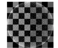
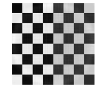
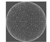
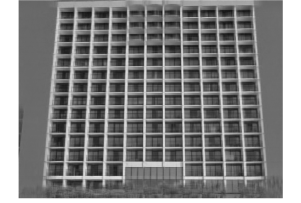
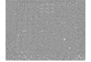
In the second experiment we implemented the CoMP algorithm to decompose real images and extract the underlying low rank/sparse singular distortion/smooth background components. The purpose of these experiments is to illustrate how the algorithm performs with the choice of small regularization parameters which is meaningful from the point of view of applications to image recovery. Image decomposition results for two images are provided on figures 1 and 2. On figure 1 we present the decomposition of the observed image of size . We apply the model (59) with regularization parameters . We run iterations of CoMP (total of sec MATLAB, Intel i5-2400S @2.5GHz CPU). The first component has approximate rank ; the relative error of the reconstruction .
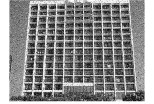
Figure 2 shows the decomposition of the observed image of size after iterations of CoMP (CPU sec). The regularization parameters of the model (59) were set to .
The relative error of the reconstruction .


5 Semi-Separable Convex Problems
5.1 Preliminaries
Our problem of interest in this section is problem (4), (6), namely,
| (66) |
where is some norm and is the conjugate norm. A straightforward approach to (66) would be to rewrite it as a saddle point problem
| (67) |
and solve by the mirror-prox algorithm from section 3.2 adjusted to work with an unbounded domain , or, alternatively, we could replace with with “large enough” and use the above algorithm “as is.” The potential problem with this approach is that if the -component of the saddle point of (67) is of large -norm (or “large enough” is indeed large), the (theoretical) efficiency estimate would be bad since it is proportional to the magnitude of (resp., to ). To circumvent this difficulty, we apply to (66) the sophisticated policy originating from [15]. This policy requires the set to be bounded, which we assume below.
Course of actions.
Note that our problem of interest is of the generic form
| (68) |
where is a convex compact set in a Euclidean space , and are convex and Lipschitz continuous functions. For the time being, we focus on (68) and assume that the problem is feasible and thus solvable.
We intend to solve (68) by the generic algorithm presented in [15]; for our now purposes, the following description of the algorithm will do:
-
1.
The algorithm works in stages. Stage is associated with working parameter . We set .
-
2.
At stage , we apply a first order method to the problem
(69) The only property of the algorithm which matters here is its ability, when run on , to produce in course of steps iterates , upper bounds on and lower bounds on in such a way that
-
(a)
for every , the -th iterate of as applied to belongs to ;
-
(b)
the upper bounds are nonincreasing in (this is “for free”) and “are achievable,” that is, they are of the form
where is a vector which we have at our disposal at step of stage ;
-
(c)
the lower bounds should be nondecreasing in t (this again is “for free”);
-
(d)
for some nonincreasing sequence , , we should have
for all and .
Note that since (68) is solvable, we clearly have , implying that the quantity is a lower bound on Opt. Thus, at step of stage we have at our disposal a number of valid lower bounds on Opt; we denote the best (the largest) of these bounds , so that
(70) for all , and is nondecreasing in time777in what follows, we call a collection of reals nonincreasing in time, if whenever , same as whenever and . “Nondecreasing in time” is defined similarly..
-
(a)
-
3.
When the First Order oracle is invoked at step of stage , we get at our disposal a triple . We assume that all these triples are somehow memorized. Thus, after calling First Order oracle at step of stage , we have at our disposal a finite set on the 2D plane such that for every point we have at our disposal a vector such that and ; the set (in today terminology, a filter) is comprised of all pairs generated so far. We set
(71) -
4.
Let , so that is a segment in . Unless we have arrived at (i.e., got an optimal solution to (68), see (72)), is not a singleton (since otherwise were 0). Observe also that are nested: whenever , same as whenever and .
We continue iterations of stage while is “well-centered” in , e.g., belongs to the mid-third of the segment. When this condition is violated, we start stage , specifying as the midpoint of .
The properties of the aforementioned routine are summarized in the following statement (cf. [15]).
Proposition 5.1
(i) is nonincreasing in time. Furthermore, at step of stage , we have at our disposal a solution to (68) such that
| (72) |
so that belongs to the domain of problem (68) and is both -feasible and -optimal.
(ii) For every , the number of stages until a pair with is found obeys the bound
| (73) |
where is an a priori upper bound on . Besides this, the number of steps at each stage does not exceed
| (74) |
5.2 Composite Mirror Prox algorithm for Semi-Separable Optimization
Problem setup
we consider now is as follows (cf. section 4.1). For every , , we are given
-
1.
Euclidean spaces and along with their nonempty closed and bounded convex subsets and , respectively;
-
2.
proximal setups for and , that is, norms on , norms on , and d.g.f.’s , , which are compatible with and , respectively;
-
3.
linear mapping , where is a Euclidean space;
-
4.
Lipschitz continuous convex functions along with their saddle point representations
(75) where are smooth (with Lipschitz continuous gradients) functions convex in and concave in , and are Lipschitz continuous convex functions such that the problems of the form
(76) are easy to solve;
-
5.
Lipschitz continuous convex functions such that the problems of the form
are easy to solve;
-
6.
a norm on , with conjugate norm , along with a d.g.f. compatible with and is such that problems of the form
are easy to solve.
The outlined data define the sets
The problem of interest here is problem (66), (75):
| (79) | |||
| (82) |
Solving (82)
using the approach in the previous section amounts to resolving a sequence of problems as in (69) where, with a slight abuse of notation,
Here are finite constants introduced to make compact, as required in the premise of Proposition 5.1; it is immediately seen that the magnitudes of these constants (same as their very presence) does not affect the algorithm we are about to describe.
The algorithm we intend to use will solve by reducing the problem to the saddle point problem
| (85) |
where .
Setting
can be thought of as the domain of the variational inequality associated with (85), the monotone operator in question being
| (86) |
By exactly the same reasons as in section 4, with properly assembled norm on the embedding space of and d.g.f., (85) can be solved by the Mirror Prox algorithm from section 3.2. Let us denote
the approximate solution obtained in course of steps of CoMP when solving , and let
be the corresponding value of the objective of . It holds
| (87) |
where is explicitly given by the proximal setup we use and by the related Lipschitz constant of (note that this constant can be chosen to be independent of ). We assume that computing the corresponding objective value is a part of step (these computations increase the complexity of a step by factor at most ), and thus that . By (87), the quantity is a valid lower bound on the optimal value of , and thus we can ensure that . The bottom line is that with the outlined implementation, we have
for all , with given by (87). Consequently, by Proposition 5.1, the total number of CoMP steps needed to find a belonging to the domain of the problem of interest (66) -feasible and -optimal solution to this problem can be upper-bounded by
where and are readily given by the smoothness parameters of and by the proximal setup we use.
5.3 Numerical illustration: -minimization
Problem of interest.
We consider the simple minimization problem
| (88) |
where , and . Note that this problem can also be written in the semi-separable form
if the data is partitioned into blocks: and .
Our main purpose here is to test the approach described in 5.1 and compare it to the simplest approach where we directly apply CoMP to the (saddle point reformulation of the) problem with large enough value of . For the sake of simplicity, we work with the case when and .
Generating the data.
In the experiments to be reported, the data of (88) were generated as follows. Given , we first build a sparse solution by drawing random vector from the standard Gaussian distribution , zeroing out part of the entries and scaling the resulting vector to enforce . We also build a dual solution by scaling a random vector from distribution to satisfy for a prescribed . Next we generate and such that and are indeed the optimal primal and dual solutions to the minimization problem (88), i.e. and . To achieve this, we set
where , and is a submatrix randomly selected from the DFT matrix . We expect that the larger is the -norm of the dual solution, the harder is problem (88).
Implementing the algorithm.
When implementing the algorithm from section 5.2, we apply at each stage CoMP to the saddle point problem
The proximal setup for CoMP is given by equipping the embedding space of with the norm and equipping with the d.g.f. . In the sequel we refer to the resulting algorithm as sequential CoMP. For comparison, we solve the same problem by applying CoMP to the saddle point problem
with ; the resulting algorithm is referred to as simple CoMP. Both sequential CoMP and simple CoMP algorithms are terminated when the relative nonoptimality and constraint violation are both less than , namely,
| sequential CoMP | simple CoMP | |||||
|---|---|---|---|---|---|---|
| steps | CPU(sec) | steps | CPU(sec) | |||
| 1024 | 512 | 1 | 7653 | 18.68 | 31645 | 67.78 |
| 5 | 43130 | 44.66 | 90736 | 90.67 | ||
| 10 | 48290 | 49.04 | 93989 | 93.28 | ||
| 4096 | 2048 | 1 | 28408 | 85.83 | 46258 | 141.10 |
| 5 | 45825 | 199.96 | 93483 | 387.88 | ||
| 10 | 52082 | 179.10 | 98222 | 328.31 | ||
| 16384 | 8192 | 1 | 43646 | 358.26 | 92441 | 815.97 |
| 5 | 48660 | 454.70 | 93035 | 784.05 | ||
| 10 | 55898 | 646.36 | 101881 | 1405.80 | ||
| 65536 | 32768 | 1 | 45153 | 3976.51 | 92036 | 4522.43 |
| 5 | 55684 | 4138.62 | 100341 | 8054.35 | ||
| 10 | 69745 | 6214.18 | 109551 | 9441.46 | ||
| 262144 | 131072 | 1 | 46418 | 6872.64 | 96044 | 14456.99 |
| 5 | 69638 | 10186.51 | 109735 | 16483.62 | ||
| 10 | 82365 | 12395.67 | 95756 | 13634.60 | ||
Numerical results
are presented in Table 4. One can immediately see that to achieve the desired accuracy, the simple CoMP with set to , i.e., to the exact magnitude of the true Lagrangian multiplier, requires almost twice as many steps as the sequential CoMP. In more realistic examples, the simple CoMP will additionally suffer from the fact that the magnitude of the optimal Lagrange multiplier is not known in advance, and the penalty in should be somehow tuned “online.”
References
- [1] E. D. Andersen and K. D. Andersen. The MOSEK optimization tools manual. http://www.mosek.com/fileadmin/products/6_0/tools/doc/pdf/tools.pdf.
- [2] J.-F. Aujol and A. Chambolle. Dual norms and image decomposition models. International Journal of Computer Vision, 63(1):85–104, 2005.
- [3] A. Beck and M. Teboulle. A fast iterative shrinkage-thresholding algorithm for linear inverse problems. SIAM Journal on Imaging Sciences, 2(1):183–202, 2009.
- [4] S. Becker, J. Bobin, and E. J. Candès. Nesta: a fast and accurate first-order method for sparse recovery. SIAM Journal on Imaging Sciences, 4(1):1–39, 2011.
- [5] S. Boyd, N. Parikh, E. Chu, B. Peleato, and J. Eckstein. Distributed optimization and statistical learning via the alternating direction method of multipliers. Foundations and Trends® in Machine Learning, 3(1):122–122, 2010.
- [6] A. Buades, B. Coll, and J.-M. Morel. A review of image denoising algorithms, with a new one. Multiscale Modeling & Simulation, 4(2):490–530, 2005.
- [7] E. J. Candés, X. Li, Y. Ma, and J. Wright. Robust principal component analysis? Journal of the ACM (JACM), 58(3):11, 2011.
- [8] A. Chambolle and T. Pock. A first-order primal-dual algorithm for convex problems with applications to imaging. Journal of Mathematical Imaging and Vision, 40(1):120–145, 2011.
- [9] G. Chen and M. Teboulle. Convergence analysis of a proximal-like minimization algorithm using bregman functions. SIAM Journal on Optimization, 3(3):538–543, 1993.
- [10] W. Deng, M.-J. Lai, Z. Peng, and W. Yin. Parallel multi-block admm with o (1/k) convergence, 2013. http://www.optimization-online.org/DB_HTML/2014/03/4282.html.
- [11] D. Goldfarb and S. Ma. Fast multiple-splitting algorithms for convex optimization. SIAM Journal on Optimization, 22(2):533–556, 2012.
- [12] D. Goldfarb, S. Ma, and K. Scheinberg. Fast alternating linearization methods for minimizing the sum of two convex functions. Mathematical Programming, 141(1-2):349–382, 2013.
- [13] M. Grant, S. Boyd, and Y. Ye. Cvx: Matlab software for disciplined convex programming, 2008.
- [14] A. Juditsky and A. Nemirovski. First-order methods for nonsmooth largescale convex minimization: I general purpose methods; ii utilizing problems structure. In S. Sra, S. Nowozin, and S. Wright, editors, Optimization for Machine Learning, pages 121–183. The MIT Press, 2011.
- [15] C. Lemaréchal, A. Nemirovskii, and Y. Nesterov. New variants of bundle methods. Mathematical Programming, 69(1-3):111–147, 1995.
- [16] R. D. Monteiro and B. F. Svaiter. Iteration-complexity of block-decomposition algorithms and the alternating direction method of multipliers. SIAM Journal on Optimization, 23(1):475–507, 2013.
- [17] A. Nemirovski. Prox-method with rate of convergence o (1/t) for variational inequalities with lipschitz continuous monotone operators and smooth convex-concave saddle point problems. SIAM Journal on Optimization, 15(1):229–251, 2004.
- [18] A. Nemirovski, S. Onn, and U. G. Rothblum. Accuracy certificates for computational problems with convex structure. Mathematics of Operations Research, 35(1):52–78, 2010.
- [19] A. Nemirovski and R. Rubinstein. An efficient stochastic approximation algorithm for stochastic saddle point problems. In M. Dror, P. L’Ecuyer, and F. Szidarovszky, editors, Modeling Uncertainty and examination of stochastic theory, methods, and applications, pages 155–184. Kluwer Academic Publishers, 2002.
- [20] Y. Nesterov. Gradient methods for minimizing composite functions. Mathematical Programming, 140(1):125–161, 2013.
- [21] F. Orabona, A. Argyriou, and N. Srebro. Prisma: Proximal iterative smoothing algorithm. arXiv preprint arXiv:1206.2372, 2012.
- [22] Y. Ouyang, Y. Chen, G. Lan, and E. Pasiliao Jr. An accelerated linearized alternating direction method of multipliers, 2014. http://arxiv.org/abs/1401.6607.
- [23] Z. Qin and D. Goldfarb. Structured sparsity via alternating direction methods. The Journal of Machine Learning Research, 13:1373–1406, 2012.
- [24] K. Scheinberg, D. Goldfarb, and X. Bai. Fast first-order methods for composite convex optimization with backtracking. http://www.optimization-online.org/DB_FILE/2011/04/3004.pdf, 2011. http://www.optimization-online.org/DB_FILE/2011/04/3004.pdf.
- [25] P. Tseng. Alternating projection-proximal methods for convex programming and variational inequalities. SIAM Journal on Optimization, 7(4):951–965, 1997.
- [26] P. Tseng. On accelerated proximal gradient methods for convex-concave optimization. submitted to SIAM Journal on Optimization, 2008.
- [27] Z. Wen, D. Goldfarb, and W. Yin. Alternating direction augmented lagrangian methods for semidefinite programming. Mathematical Programming Computation, 2(3-4):203–230, 2010.
Appendix A Proof of Theorem 3.1
0o.
Let us verify that the prox-mapping (28) indeed is well defined whenever with . All we need is to show that whenever , , and , , are such that as , we have
Indeed, assuming the opposite and passing to a subsequence, we make the sequence bounded. Since is strongly convex, modulus 1, w.r.t. , and the linear function of is below bounded on by A4, boundedness of the sequence implies boundedness of the sequence , and since as , we get as . Since is coercive in on by A4, and , we conclude that , , while the sequence is bounded since the sequence is so and is continuously differentiable. Thus, is bounded, , , implying that , , which is the desired contradiction
1o
2o.
When applying (90) with , , , and we obtain:
| (91) |
and applying (90) with , , , and we get:
| (92) |
Adding (92) to (91) we obtain for every
| (93) | |||||
Due to the strong convexity, modulus 1, of w.r.t. , for all . Therefore,
where the last inequality is due to (23). Note that implies that
Let us assume that the stepsizes ensure that (30) holds, meaning that (which, by the above analysis, is definitely the case when ; when , we can take also ). When summing up inequalities (93) over and taking into account that , we conclude that for all ,
Appendix B Proof of Lemma 3.1
Proof. All we need to verify is the second inequality in (38). To this end note that when , the inequality in (38) holds true by definition of . Now let . Summing up the inequalities (93) over , we get for every :
(we have used (30)). When is , the left hand side in the resulting inequality is , and we arrive at
whence
whence also
and therefore
| (94) |
and (38) follows.
Appendix C Proof of Proposition 3.1
Appendix D Proof of Proposition 5.1
1o.
are concave piecewise linear functions on which clearly are pointwise nonincreasing in time. As a result, is nonincreasing in time. Further, we have
where and sum up to 1. Recalling that for every we have at our disposal such that and , setting and invoking convexity of , we get
and (72) follows, due to .
2o.
We have for some which we have at our disposal at step , implying that . Hence by definition of it holds
where the concluding inequality is given by (70). Thus, . On the other hand, if stage does not terminate in course of the first steps, is well-centered in the segment where the concave function is nonnegative. We conclude that . Thus, if a stage does not terminate in course of the first steps, we have , which implies (74). Further, is the midpoint of the segment , where is the last step of stage (when , we should define as ), and is not well-centered in the segment , which clearly implies that . Thus, for all . On the other hand, when , we have (since is Lipschitz continuous with constant 888we assume w.l.o.g. that and vanishes at (at least) one endpoint of ). Thus, the number of stages before is reached indeed obeys the bound (73).