The scalar mesons in multi-channel $\pi\pi$ scattering and decays of the $\psi$ and $\Upsilon$ families

Abstract

The $f_{0}$ mesons are studied in a combined analysis of data on the isoscalar S-wave processes $\pi\pi\to\pi\pi,K\overline{K},\eta\eta$ and on decays $J/\psi\to\phi(\pi\pi,K\overline{K})$, $\psi(2S)\to J/\psi(\pi\pi)$, and $\Upsilon(2S)\to\Upsilon(1S)\pi\pi$ from the Argus, Crystal Ball, CLEO, CUSB, DM2, Mark II, Mark III, and BES II collaborations. The method of analysis, based on analyticity and unitarity and using an uniformization procedure, is set forth with some details. Some spectroscopic implications from results of the analysis are discussed.

I Introduction

The problem of scalar mesons, particularly their nature, parameters, and status of some of them, is still not solved PDG12 . E.g., applying our method of the uniformizing variable in the 3-channel analyses of multi-channel $\pi\pi$ scattering SBKN-PRD10 ; SBL-PRD12 we have obtained parameters of the $f_{0}(500)$ and $f_{0}(1500)$ which differ considerably from results of analyses utilizing other methods (mainly based on dispersion relations or Breit-Wigner approaches). Reasons for this difference were understood in our works SBKLN-PRD12 ; SBKLN-1206_3438 ; SBKLN-1207_6937 . We have shown that when studying wide multi-channel resonances, as the scalar ones, the Riemann-surface structure of the $S$-matrix of considered processes must be allowed for properly. For the scalar states this is, as minimum, the 8-sheeted Riemann surface. This is related with a necessity to analyze jointly coupled processes $\pi\pi\to\pi\pi,K\overline{K},\eta\eta$ because, as it was shown, studying only $\pi\pi$ scattering it is impossible to obtain correct values for parameters of the scalar states. Calculating masses, total widths and coupling constants of resonances with channels, one must use the poles on sheets II, IV and VIII, depending on the state type.

From these results an important conclusion can be drawn: Even if a wide resonance does not decay into a channel which opens above its mass but it is strongly connected with this channel, one ought to consider this state taking into account the Riemann-surface sheets related to the threshold branch-point of this channel. I.e., the dispersion relation approach in which amplitudes are considered only on the 2-sheeted Riemann surface does not suit for correct determination of this resonance parameters.

Note importance of our above-indicated conclusions because our approach is based only on the demand for analyticity and unitarity of the amplitude using an uniformization procedure. The construction of the amplitude is essentially free from any dynamical (model) assumptions utilizing only the mathematical fact that a local behaviour of analytic functions determined on the Riemann surface is governed by the nearest singularities on all corresponding sheets. Therefore it seems that our approach permits us to omit theoretical prejudice in extracting the resonance parameters.

Analyzing only $\pi\pi\to\pi\pi,K\overline{K},\eta\eta(\eta\eta^{\prime})$ SBL-PRD12 in the 3-channel approach, we have shown that experimental data on the $\pi\pi$ scattering below 1 GeV admit two possibilities for parameters of the $f_{0}(500)$ with mass, relatively near to the $\rho$-meson mass, and with the total widths about 600 and 950 MeV – solutions “A” and “B”, respectively.

Furthermore, it was shown that for the states $f_{0}(1370)$, $f_{0}(1500)$ (as a superposition of two states, broad and narrow), and $f_{0}(1710)$, there are four scenarios of possible representation by poles and zeros on the Riemann surface giving similar descriptions of the above processes and, however, quite different parameters of some resonances. E.g., for the $f_{0}(500)$ (A solution), $f_{0}(1370)$ and $f_{0}(1710)$, a following spread of values is obtained for the masses and total widths respectively: 605-735 and 567-686 MeV, 1326-1404 and 223-345 MeV, and 1751-1759 and 118-207 MeV.

Adding to the combined analysis the data on decays $J/\psi\to\phi(\pi\pi,K\overline{K})$ from the Mark III, DM2 and BES II collaborations Mark_III , we have considerably diminished a quantity of the possible scenarios SBKLN-1207_6937 . Moreover the di-pion mass distribution in the $J/\psi\to\phi\pi\pi$ decay of the BES II data from the threshold to about 850 MeV prefers surely the solution with the wider $f_{0}(500)$ – B-solution. This is a problem because most of physicists PDG12 prefer a narrower $f_{0}(500)$. Therefore, here we expanded our combined analysis adding also accessible data on the decays $\psi(2S)\to J/\psi(\pi\pi)$ and $\Upsilon(2S)\to\Upsilon(1S)\pi\pi$ from the Argus, Crystal Ball, CLEO, CUSB, and Mark II collaborations Mark_II ; Argus .

There are also other problems related to interpretation of scalar mesons, e.g., as to an assignment of the scalar mesons to lower $q{\bar{q}}$ nonets. There is a number of properties of the scalar mesons, which do not allow to make up satisfactorily the lowest nonet. The main of them is inaccordance of the approximately equal masses of the $f_{0}(980)$ and $a_{0}(980)$ and the found $s{\bar{s}}$ dominance in the wave function of the $f_{0}(980)$. If these states are in the same nonet, the $f_{0}(980)$ must be heavier by 250-300 MeV than $a_{0}(980)$ because the difference of masses of $s$- and $u$-quarks is 120-150 MeV. In connection with this, various variants for solution are proposed. The most popular one is the 4-quark interpretation of ${f_{0}}(980)$ and ${a_{0}}(980)$ mesons, in favour of which as though additional arguments have been found on the basis of interpretation of the experimental data on the decays $\phi\to\gamma\pi^{0}\pi^{0},\gamma\pi^{0}\eta$ Achasov-4q . However, the 4-quark model, beautifully solving the old problem of the unusual properties of scalar mesons, sets new questions. Where are the 2-quark states, their radial excitations and the other members of 4-quark multiplets $9,9^{*},36$ and $36^{*}$, which are predicted to exist below 2.5 GeV Jaffe-4q ? We proposed our way to solve this problem.

Existence of the $f_{0}(1370)$ meson is still not obvious. In some works, e.g., in MO-02-2 ; Ochs10 one did not find any evidence for the existence of the $f_{0}(1370)$. On the other hand, in Ref. Bugg1370 a number of data requiring apparently the existence of the $f_{0}(1370)$ is indicated. We have shown SBL-PRD12 that an existence of the $f_{0}(1370)$ does not contradict the data on processes $\pi\pi\to\pi\pi,K\overline{K},\eta\eta(\eta\eta^{\prime})$ and if this state exists, it has a dominant $s{\bar{s}}$ component. In the hidden gauge unitary approach, the $f_{0}(1370)$ appears dynamically generated as a $\rho\rho$ state Geng_Oset and the $f_{0}(1710)$ as generated from the $K^{\ast}\bar{K}^{\ast}$ interaction.

Further we shall consider mainly the 3-channel case because it was shown that this is a minimal number of channels needed for obtaining correct values of scalar resonance parameters. However for convenience and having in mind other problems, we shall mention sometimes the 2- and N-channel cases.

II Method of the uniformizing variable in the 3-channel $\pi\pi$ scattering

Our model-independent method which essentially utilizes a uniformizing variable can be used only for the 2-channel case and under some conditions for the 3-channel one. Only in these cases we obtain a simple symmetric (easily interpreted) picture of the resonance poles and zeros of the $S$-matrix on the uniformization plane. The 2- or 3-channel $S$-matrix is determined on the 4- or 8-sheeted Riemann surface, respectively. The matrix elements $S_{ij}$, where $i,j=1,2,3$ denote channels, have the right-hand cuts along the real axis of the $s$ complex plane ($s$ is the invariant total energy squared), starting with the channel thresholds $s_{i}$ ($i=1,2,3$), and the left-hand cuts related to the crossed channels. The Riemann-surface sheets, denoted by the Roman numbers, are numbered according to the signs of analytic continuations of the square roots $\sqrt{s-s_{i}}$ as follows

	I	II	III	IV	V	VI	VII	VIII
$\mbox{Im}\sqrt{s-s_{1}}$	$+$	$-$	$-$	$+$	$+$	$-$	$-$	$+$
$\mbox{Im}\sqrt{s-s_{2}}$	$+$	$+$	$-$	$-$	$-$	$-$	$+$	$+$
$\mbox{Im}\sqrt{s-s_{3}}$	$+$	$+$	$+$	$+$	$-$	$-$	$-$	$-$

The sewing together of the Riemann surface sheets is shown in Fig. 1.

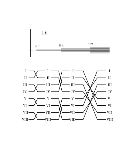
Figure 1: Sewing together the sheets of the Riemann surface.

Our approach is based on general principles, as analyticity and unitarity, and realizes an idea of the consistent account of the nearest (to the physical region) singularities on all sheets of the Riemann surface of the $S$-matrix, thus giving a chance to obtain a model-independent information on multi-channel resonances from the analysis of data on the coupled processes. The main model-independent contribution of resonances is given by poles and corresponding zeros on the Riemann surface. A reasonable and simple description of the background should be a criterion of correctness of this statement. Obviously, we deal with renormalized quantities, and the poles of S-matrix correspond to dressed particles.

If a resonance has the only decay mode (1-channel case), the general statement about a behaviour of the process amplitude is that at energy values in a proximity to the resonance the amplitude describes the propagation of resonance as if it is a free particle. This means that in the matrix element the resonance (in the limit of its narrow width) is represented by a pair of complex conjugate poles on sheet II and by a pair of conjugate zeros on the physical sheet at the same points of complex energy. This model-independent statement about the poles as the nearest singularities holds also when taking account of the finite width of a resonance. Obviously, the statement that the poles corresponding to resonances are the nearest (to the physical region) singularities holds also in the multi-channel case.

In order to obtain an arrangement of poles and zeros of multi-channel resonance on the Riemann surface, we use the proved fact that on the physical sheet, the $S$-matrix elements can possess only the resonance zeros (beyond the real axis), at least, around the physical region. Therefore it is necessary to obtain formulas expressing analytic continuations of the $S$-matrix elements to all sheets in terms of those on the physical sheet KMS-nc96 .

To this end, let us consider the $N$-channel $S$-matrix (all channels are two-particle ones) determined on the $2^{N}$-sheeted Riemann surface. The Riemann surface has the right-hand (unitary) cuts along the real axis of the $s$-variable complex plane $(s_{i},\infty)$  ($i=1,2,\cdots,N$ means a channel) through which the physical sheet is sewed together with other sheets. The branch points are at the vanishing values of the channel momenta  ${k_{\alpha}}=(s/4-m_{\alpha}^{2})^{1/2}$. For now we will neglect the left-hand cut in the Riemann-surface structure related with the crossing-channel contributions, whose contribution, in principle, can be taken into account in the background of the corresponding amplitudes.

In the following it is convenient to use enumeration of sheets (see, e.g., Kato-AP65 ): the physical sheet is denoted as $L_{0}$, other sheets through $L_{i_{1}\cdots i_{k}}$ where  $i_{1}\cdots i_{k}$  are a system of subscripts of those channel-momenta $k_{i_{n}}$ which change signs at analytical continuations from the physical sheet onto the indicated one. Then the analytical continuations of $S$-matrix elements $S_{ik}$ to the unphysical sheet $L_{i_{1}\cdots i_{k}}$ are $S_{ik}^{(i_{1}\cdots i_{k})}$. We will obtain the formula expressing $S_{ik}^{(i_{1}\cdots i_{k})}$ in terms of $S_{ik}^{(0)}$ (matrix elements $S_{ik}$ on the physical sheet $L_{0}$), using the reality property of the analytic functions and the $N$-channel unitarity. The direct derivation of these formulas requires rather bulky algebra. It can be simplified if we use Hermiticity of the $K$-matrix.

To this end, first, we shall introduce the notation:  ${\bf S}^{[i_{1}\cdots i_{k}]}$  means a matrix in which all the rows are composed of the vanishing elements but the rows $i_{1},\cdots,i_{k},$ that consist of elements $S_{i_{n}i_{m}}$. In the matrix  ${\bf S}^{\{i_{1}\cdots i_{k}\}}$, on the contrary, the rows $i_{1},\cdots,i_{k}$ are zeros. Therefore,

$${\bf S}^{[i_{1}\cdots i_{k}]}+{\bf S}^{\{i_{1}\cdots i_{k}\}}={\bf S}.$$ (1)

Further  ${\bf\Delta}^{[i_{1}\cdots i_{k}]}$  and  ${\bf\Delta}^{\{i_{1}\cdots i_{k}\}}$  denote the diagonal matrices with the elements

$$\Delta_{ii}^{[i_{1}\cdots i_{k}]}=\left\{\begin{array}[]{l}1\quad\mbox{if}~{}~{}i\in(i_{1}\cdots i_{k}),\\ 0\quad\mbox{for remaining}~{}~{}i,\end{array}\right.\quad\mbox{and}\quad\Delta_{ii}^{\{i_{1}\cdots i_{k}\}}=\left\{\begin{array}[]{l}0\quad\mbox{if}~{}~{}i\in(i_{1}\cdots i_{k}),\\ 1\quad\mbox{for remaining}~{}~{}i,\end{array}\right.$$

respectively. Further using relation of the $S$- and $K$-matrices

$${\bf S}=\frac{I+i{\bf\rho}^{1/2}{\bf K}{\bf\rho}^{1/2}}{I-i{\bf\rho}^{1/2}{\bf K}{\bf\rho}^{1/2}}~{}~{}~{}{\rm where}~{}~{}\rho_{ij}=0~{}(i\neq j),~{}~{}\rho_{ii}={2k_{i}}/{\sqrt{s}}$$ (2)

and  ${\bf S}{\bf S}^{+}={\bf I}$, it is easy to obtain that ${\bf K}={\bf K}^{+}$, i.e., the $K$-matrix has no discontinuity when going across the two-particle unitary cuts and has the same value in all sheets of the Riemann surface of the $S$-matrix. Using the latter fact, we obtain the needed formula. The analytical continuations of the $S$-matrix to the sheet $L_{i_{1}\cdots i_{k}}$ will be represented as

$${\bf S}^{(i_{1}\cdots i_{k})}=\frac{{\bf S}^{(0)\{i_{1}\cdots i_{k}\}}-i{\bf\Delta}^{[i_{1}\cdots i_{k}]}}{{\bf\Delta}^{\{i_{1}\cdots i_{k}\}}-i{\bf S}^{(0)[i_{1}\cdots i_{k}]}}.$$ (3)

From the last formula the corresponding relations for the $S$-matrix elements can be derived by the formula for the matrix division. In Table 1 the result is shown for the 3-channel case. We have returned to more standard enumeration of sheets by Roman numerals I, II,…,VIII.

	$L_{0}$	$L_{1}$	$L_{12}$	$L_{2}$	$L_{23}$	$L_{123}$	$L_{13}$	$L_{3}$
Process	I	II	III	IV	V	VI	VII	VIII
$1\to 1$	$S_{11}$	$\frac{1}{S_{11}}$	$\frac{S_{22}}{D_{33}}$	$\frac{D_{33}}{S_{22}}$	$\frac{\det S}{D_{11}}$	$\frac{D_{11}}{\det S}$	$\frac{S_{33}}{D_{22}}$	$\frac{D_{22}}{S_{33}}$
$1\to 2$	$S_{12}$	$\frac{iS_{12}}{S_{11}}$	$\frac{-S_{12}}{D_{33}}$	$\frac{iS_{12}}{S_{22}}$	$\frac{iD_{12}}{D_{11}}$	$\frac{-D_{12}}{\det S}$	$\frac{iD_{12}}{D_{22}}$	$\frac{D_{12}}{S_{33}}$
$2\to 2$	$S_{22}$	$\frac{D_{33}}{S_{11}}$	$\frac{S_{11}}{D_{33}}$	$\frac{1}{S_{22}}$	$\frac{S_{33}}{D_{11}}$	$\frac{D_{22}}{\det S}$	$\frac{\det S}{D_{22}}$	$\frac{D_{11}}{S_{33}}$
$1\to 3$	$S_{13}$	$\frac{iS_{13}}{S_{11}}$	$\frac{-iD_{13}}{D_{33}}$	$\frac{-D_{13}}{S_{22}}$	$\frac{-iD_{13}}{D_{11}}$	$\frac{D_{13}}{\det S}$	$\frac{-S_{13}}{D_{22}}$	$\frac{iS_{13}}{S_{33}}$
$2\to 3$	$S_{23}$	$\frac{D_{23}}{S_{11}}$	$\frac{iD_{23}}{D_{33}}$	$\frac{iS_{23}}{S_{22}}$	$\frac{-S_{23}}{D_{11}}$	$\frac{-D_{23}}{\det S}$	$\frac{iD_{23}}{D_{22}}$	$\frac{iS_{23}}{S_{33}}$
$3\to 3$	$S_{33}$	$\frac{D_{22}}{S_{11}}$	$\frac{\det S}{D_{33}}$	$\frac{D_{11}}{S_{22}}$	$\frac{S_{22}}{D_{11}}$	$\frac{D_{33}}{\det S}$	$\frac{S_{11}}{D_{22}}$	$\frac{1}{S_{33}}$

Table 1: Analytic continuations of the 3-channel $S$-matrix elements to unphysical sheets.

In Table 1, the superscript $I$ is omitted to simplify the notation, $\det S$ is the determinant of the $3\times 3$ $S$-matrix on sheet I, $D_{\alpha\beta}$ is the minor of the element $S_{\alpha\beta}$, that is, $D_{11}=S_{22}S_{33}-S_{23}^{2}$, $D_{22}=S_{11}S_{33}-S_{13}^{2}$, $D_{33}=S_{11}S_{22}-S_{12}^{2}$, $D_{12}=S_{12}S_{33}-S_{13}S_{23}$, $D_{23}=S_{11}S_{23}-S_{12}S_{13}$, etc.

These formulas show how singularities and resonance poles and zeros are transferred from the matrix element $S_{11}$ to matrix elements of coupled processes. Starting from the resonance zeros on sheet I, one can obtain the arrangement of poles and zeros of resonance on the whole Riemann surface.

Let us explain in the 2-channel example how a pole cluster describing resonance arises. In the 1-channel consideration of the scattering $1\to 1$ the main model-independent contribution of resonance is given by a pair of conjugate poles on sheet II and by a pair of conjugate zeros on sheet I at the same points of complex energy in $S_{11}$. (Conjugate poles and zeros are needed for real analyticity.) In the 2-channel consideration of the processes $1\to 1$, $1\to 2$ and $2\to 2$, we have

$$S_{11}^{\rm II}=\frac{1}{S_{11}^{\rm I}},\qquad~{}~{}~{}~{}~{}~{}~{}~{}~{}~{}~{}~{}~{}S_{11}^{\rm III}=\frac{S_{22}^{\rm I}}{S_{11}^{\rm I}S_{22}^{I}-(S_{12}^{\rm I})^{2}},\quad S_{11}^{\rm IV}=\frac{S_{11}^{\rm I}S_{22}^{\rm I}-(S_{12}^{\rm I})^{2}}{S_{22}^{I}},$$ (4)

$$S_{22}^{\rm II}=\frac{S_{11}^{\rm I}S_{22}^{\rm I}-(S_{12}^{\rm I})^{2}}{S_{11}^{\rm I}},\quad S_{22}^{\rm III}=\frac{S_{11}^{\rm I}}{S_{11}^{\rm I}S_{22}^{\rm I}-(S_{12}^{\rm I})^{2}},\quad S_{22}^{\rm IV}=\frac{1}{S_{22}^{\rm I}},$$ (5)

$$S_{12}^{\rm II}=\frac{iS_{12}^{\rm I}}{S_{11}^{\rm I}},\qquad~{}~{}~{}~{}~{}~{}~{}~{}~{}~{}~{}~{}~{}S_{12}^{\rm III}=\frac{-S_{12}^{\rm I}}{S_{11}^{\rm I}S_{22}^{\rm I}-(S_{12}^{\rm I})^{2}},\quad S_{12}^{\rm IV}=\frac{iS_{12}^{\rm I}}{S_{22}^{\rm I}}.$$ (6)

In $S_{11}$ a resonance is represented by a pair of conjugate poles on sheet II and by a pair of conjugate zeros on sheet I and also by a pair of conjugate poles on sheet III and by a pair of conjugate zeros on sheet IV at the same points of complex energy if the coupling of channels is absent ($S_{12}=0$). If the resonance decays into both channels and/or takes part in exchanges in the crossing channels, the coupling of channels arises ($S_{12}\not=0$). Then positions of the poles on sheet III (and of corresponding zeros on sheet IV) turn out to be shifted with respect to the positions of zeros on sheet I. Thus we obtain the cluster (of type (a)) of poles and zeros.

In the 2-channel case, 3 types of resonances are obtained corresponding to a pair of conjugate zeros on sheet I only in $S_{11}$ – the type (a), only in $S_{22}$ – (b), and simultaneously in $S_{11}$ and $S_{22}$ – (c).
In the 3-channel case, we obtain 7 types of resonances corresponding to 7 possible situations when there are resonance zeros on sheet I only in $S_{11}$ – (a);   $S_{22}$ – (b);   $S_{33}$ – (c);   $S_{11}$ and $S_{22}$ – (d);   $S_{22}$ and $S_{33}$ – (e);   $S_{11}$ and $S_{33}$ – (f);   $S_{11}$, $S_{22}$ and $S_{33}$ – (g). The resonance of every type is represented by the pair of complex-conjugate clusters (of poles and zeros on the Riemann surface).

A necessary and sufficient condition for existence of the multi-channel resonance is its representation by one of the types of pole clusters. A main model-independent contribution of resonances is given by the pole clusters and possible remaining small (model-dependent) contributions of resonances can be included in the background. This is confirmed further by the obtained very simple description of the background.

The cluster type is related to the nature of state. E.g., if we consider the $\pi\pi$, $K\overline{K}$ and $\eta\eta$ channels, then a resonance, coupled relatively more strongly to the $\pi\pi$ channel than to the $K\overline{K}$ and $\eta\eta$ ones is described by the cluster of type (a). In the opposite case, it is represented by the cluster of type (e) (say, the state with the dominant $s{\bar{s}}$ component). The glueball must be represented by the cluster of type (g) as a necessary condition for the ideal case. Whereas cases (a), (b) and (c) can be related to the resonance representation by Breit-Wigner forms, cases (d), (e), (f) and (g) practically are lost at the Breit-Wigner description.

One can formulate a model-independent test as a necessary condition to distinguish a bound state of colorless particles (e.g., a $K\overline{K}$ molecule) and a $q{\bar{q}}$ bound state KMS-nc96 ; Morgan_Penn_93 .

In the 1-channel case, the existence of the particle bound-state means the presence of a pole on the real axis under the threshold on the physical sheet.

In the 2-channel case, existence of the bound-state in channel 2 ($K\overline{K}$ molecule) that, however, can decay into channel 1 ($\pi\pi$ decay), would imply the presence of the pair of complex conjugate poles on sheet II under the second-channel threshold without the corresponding shifted pair of poles on sheet III.

In the 3-channel case, the bound state in channel 3 ($\eta\eta$) that, however, can decay into channels 1 ($\pi\pi$ decay) and 2 ($K\overline{K}$ decay), is represented by the pair of complex conjugate poles on sheet II and by the pair of shifted poles on sheet III under the $\eta\eta$ threshold without the corresponding poles on sheets VI and VII.

According to this test, earlier we rejected interpretation of the $f_{0}(980)$ as the $K\overline{K}$ molecule because this state is represented by the cluster of type (a) in the 2-channel analysis of processes $\pi\pi\to\pi\pi,K\overline{K}$ and, therefore, does not satisfy the necessary condition to be the $K\overline{K}$ molecule KMS-nc96 .

It is convenient to use the Le Couteur-Newton relations LeCou . They express the $S$-matrix elements of all coupled processes in terms of the Jost matrix determinant $d(k_{1},\cdots,k_{N})\equiv d(s)$ that is a real analytic function with the only branch-points at $k_{i}=0$:

$$S_{ii}(s)=\frac{d^{(i)}(s)}{d(s)},$$ (7)

$$\left|{\begin{array}[]{ccc}S_{i_{1}i_{1}}(s)&\cdots&S_{i_{1}i_{k}}(s)\\ \vdots&\vdots&\vdots\\ S_{i_{k}i_{1}}(s)&\cdots&S_{i_{k}i_{k}}(s)\end{array}}\right|=\frac{d^{(i_{1}\cdots i_{k})}(s)}{d(s)}.$$ (8)

Rather simple derivation of these relations, using the $ND^{-1}$ representation of amplitudes and Hermiticity of the $K$-matrix, can be found in Ref. Kato-AP65 . The analytical structure of the $S$-matrix on all Riemann sheets given above is thus expressed in a compact way by these relations. The real analyticity implies

$$d(s^{*})=d^{*}(s)~{}~{}~{}~{}{\rm for~{}all}~{}s.$$ (9)

The unitarity condition requires further restrictions on the $d$-function for physical $s$-values which will be discussed below in the example of 3-channel $S$-matrix.

In order to use really the representation of resonances by various pole clusters, it ought to transform our multi-valued $S$-matrix, determined on the 8-sheeted Riemann surface, to one-valued function. But that function can be uniformized only on torus with the help of a simple mapping. This is unsatisfactory for our purpose. Therefore, we neglect the influence of the lowest ($\pi\pi$) threshold branch-point (however, unitarity on the $\pi\pi$ cut is taken into account). This approximation means the consideration of the nearest to the physical region semi-sheets of the Riemann surface of the $S$-matrix. In fact, we construct a 4-sheeted model of the initial 8-sheeted Riemann surface that is in accordance with our approach of a consistent account of the nearest singularities on all the relevant sheets.

In the corresponding uniformizing variable, we have neglected the $\pi\pi$-threshold branch-point and taken into account the $K\overline{K}$- and $\eta\eta$-threshold branch-points and the left-hand branch-point at $s=0$:

$$w=\frac{\sqrt{(s-s_{2})s_{3}}+\sqrt{(s-s_{3})s_{2}}}{\sqrt{s(s_{3}-s_{2})}}~{}~{}~{}~{}(s_{2}=4m_{K}^{2}~{}{\rm and}~{}s_{3}=4m_{\eta}^{2}).$$ (10)

In Figs. 2 and 3 we show the representation of resonances of all types (a), (b),…, (g) on the uniformization $w$-plane for the 3-channel-$\pi\pi$-scattering $S$-matrix element.

Figure 2: Uniformization $w$-plane for the 3-channel-$\pi\pi$-scattering matrix element. Representation of resonances of types (a), (b), (c) and (d) is shown.

Figure 3: Representation of resonances of types (e), (f), and (g).

On the $w$-plane, the Le Couteur–Newton relations are somewhat modified taking account of the used model of initial 8-sheeted Riemann surface (note that on the $w$-plane the points $w_{0}$, $-w_{0}^{-1}$, $-w_{0}$, and $w_{0}^{-1}$ correspond to the $s$-variable point $s_{0}$ on sheets I, IV, V, and VIII, respectively):

$$S_{11}=\frac{d^{*}(-w^{*})}{d(w)},~{}~{}~{}~{}~{}~{}~{}~{}S_{22}=\frac{d(-w^{-1})}{d(w)},~{}~{}~{}~{}~{}~{}~{}~{}S_{33}=\frac{d(w^{-1})}{d(w)},$$ (11)

$$S_{11}S_{22}-S_{12}^{2}=\frac{d^{*}({w^{*}}^{-1})}{d(w)},~{}~{}~{}~{}~{}~{}~{}~{}S_{11}S_{33}-S_{13}^{2}=\frac{d^{*}(-{w^{*}}^{-1})}{d(w)},~{}~{}$$ (12)

$$S_{22}S_{33}-S_{23}^{2}=\frac{d(-w)}{d(w)}.$$ (13)

Since the used model Riemann surface means only the consideration of the semi-sheets of the initial Riemann surface nearest to the physical region, then in this case there is no point in saying for the property of the real analyticity of the amplitudes. The 3-channel unitarity requires the following relations to hold for physical $w$-values:

$$|d(-w^{*})|\leq|d(w)|,\quad|d(-w^{-1})|\leq|d(w)|,\quad|d(w^{-1})|\leq|d(w)|,$$ (14)

$$|d({w^{*}}^{-1})|=|d(-{w^{*}}^{-1})|=|d(-w)|=|d(w)|.$$ (15)

The $S$-matrix elements in Le Couteur–Newton relations are taken as the products  $S=S_{B}S_{res}$; the main (model-independent) contribution of resonances, given by the pole clusters, is included in the resonance part $S_{res}$; possible remaining small (model-dependent) contributions of resonances and influence of channels which are not taken explicitly into account in the uniformizing variable are included in the background part $S_{B}$. The d-function for the resonance part is

$$d_{res}(w)=w^{-\frac{M}{2}}\prod_{r=1}^{M}(w+w_{r}^{*})$$ (16)

where $M$ is the number of resonance zeros, for the background part is

$$d_{B}=\mbox{exp}[-i\sum_{n=1}^{3}\frac{\sqrt{s-s_{n}}}{2m_{n}}(\alpha_{n}+i\beta_{n})],$$ (17)

$$\alpha_{n}=a_{n1}+a_{n\sigma}\frac{s-s_{\sigma}}{s_{\sigma}}\theta(s-s_{\sigma})+a_{nv}\frac{s-s_{v}}{s_{v}}\theta(s-s_{v}),$$

$$\beta_{n}=b_{n1}+b_{n\sigma}\frac{s-s_{\sigma}}{s_{\sigma}}\theta(s-s_{\sigma})+b_{nv}\frac{s-s_{v}}{s_{v}}\theta(s-s_{v})$$

where $s_{\sigma}$ is the $\sigma\sigma$ threshold; $s_{v}$ is the combined threshold of the $\eta\eta^{\prime}$, $\rho\rho$ and $\omega\omega$ channels.

Formalism for calculating di-meson mass distributions of the decays $J/\psi\to\phi(\pi\pi,K\overline{K})$ and $V^{\prime}\to V\pi\pi$ (e.g., $\psi(2S)\to J/\psi(\pi\pi)$ and $\Upsilon(2S)\to\Upsilon(1S)\pi\pi$) can be found in Refs. Morgan_Penn_93 ; Zou_Bugg_94 . There is assumed that pairs of pseudo-scalar mesons of final states have $I=J=0$ and only they undergo strong interactions, whereas a final vector meson ($\phi$, $V$) acts as a spectator. The amplitudes for decays are related with the scattering amplitudes $T_{ij}$ $(i,j=1-\pi\pi,2-K\overline{K})$ as follows:

$$F(J/\psi\to\phi\pi\pi)=\sqrt{2/3}~{}[c_{1}(s)T_{11}+c_{2}(s)T_{21}],$$ (18)

$$F(J/\psi\to\phi K\overline{K})=\sqrt{1/2}~{}[c_{1}(s)T_{12}+c_{2}(s)T_{22}],$$ (19)

$$F(V^{\prime}\to V\pi\pi~{}(V=\psi,\Upsilon))=[(d_{1},e_{1})T_{11}+(d_{2},e_{2})T_{21}]$$ (20)

where   $c_{1}=\gamma_{10}+\gamma_{11}s$,   $c_{2}=\alpha_{2}/(s-\beta_{2})+\gamma_{20}+\gamma_{21}s$,   and $(d_{i},e_{i})=(\delta_{i0},\rho_{i0})+(\delta_{i1},\rho_{i1})s$   are functions of couplings of the $J/\psi$, $\psi(2S)$ and $\Upsilon(2S)$ to channel $i$;  $\alpha_{2}$, $\beta_{2}$, $\gamma_{i0}$, $\gamma_{i1}$, $\delta_{i0}$, $\rho_{i0}$, $\delta_{i1}$ and $\rho_{i1}$ are free parameters. The pole term in $c_{2}$ is an approximation of possible $\phi K$ states, not forbidden by OZI rules when considering quark diagrams of these processes. Obviously this pole should be situated on the real $s$-axis below the $\pi\pi$ threshold. This is an effective inclusion of the effect of so called “crossed channel final state interactions” in $J/\psi\to\phi K\overline{K}$, which was studied largely, e.g., in Ref. Guo .

The expressions

$$N|F|^{2}\sqrt{(s-s_{i})\bigl{(}m_{\psi}^{2}-(\sqrt{s}-m_{\phi})^{2}\bigr{)}\bigl{(}m_{\psi}^{2}-(\sqrt{s}+m_{\phi})^{2}\bigr{)}}$$

for $J/\psi\to\phi\pi\pi,\phi K\overline{K}$ (and the analogues ones for $V^{\prime}\to V\pi\pi$) give the di-meson mass distributions. N (a normalization constant to data of the experiments) is 0.7512 for Mark III, 0.3705 for DM2, 5.699 for BES II, 1.015 for Mark II, 0.98 for Crystal Ball(80), 4.3439 for Argus, 2.1776 for CLEO, 1.2011 for CUSB, and 0.0788 for Crystal Ball(85).

III The combined 3-channel analysis of data on isoscalar S-wave processes $\pi\pi\to\pi\pi,K\overline{K},\eta\eta$ and on $J/\psi\to\phi(\pi\pi,K\overline{K})$, $\psi(2S)\to J/\psi(\pi\pi)$ and $\Upsilon(2S)\to\Upsilon(1S)\pi\pi$

For the data on multi-channel $\pi\pi$ scattering we used the results of phase analyses which are given for phase shifts of the amplitudes $\delta_{\alpha\beta}$ and for the modules of the $S$-matrix elements $\eta_{\alpha\beta}=|S_{\alpha\beta}|$ ($\alpha,\beta=1,~{}2,~{}3$):

$$S_{\alpha\alpha}=\eta_{\alpha\alpha}e^{2i\delta_{\alpha\alpha}},~{}~{}~{}~{}~{}S_{\alpha\beta}=i\eta_{\alpha\beta}e^{i\phi_{\alpha\beta}}.$$ (21)

If below the third threshold there is the 2-channel unitarity then the relations

$$\eta_{11}=\eta_{22},~{}~{}\eta_{12}=(1-{\eta_{11}}^{2})^{1/2},~{}~{}\phi_{12}=\delta_{11}+\delta_{22}$$ (22)

are fulfilled in this energy region.

For the $\pi\pi$ scattering, the data from the threshold to 1.89 GeV are taken from Refs. expd_pipi . For $\pi\pi\to K\overline{K}$, practically all the accessible data are used expd_pipiKK . For $\pi\pi\to\eta\eta$, we used data for $|S_{13}|^{2}$ from the threshold to 1.72 GeV expd_eta_eta . For decays $J/\psi\to\phi\pi\pi,\phi K\overline{K}$ we have taken data from Mark III , from DM2 and from BES II Mark_III ; for $\psi(2S)\to J/\psi(\pi^{+}\pi^{-})$ from Mark II and for $\psi(2S)\to J/\psi(\pi^{0}\pi^{0})$ from Crystal Ball Collaborations(80) Mark_II ; for $\Upsilon(2S)\to\Upsilon(1S)(\pi^{+}\pi^{-},\pi^{0}\pi^{0})$ from Argus, CLEO, CUSB, and Crystal Ball collaborations(85) Argus .

In this combined analyses of the coupled scattering processes and decays, it appears that to achieve a consistency with the PDG tables (to have a narrow state) it is necessary to consider two states in the 1500-MeV region – the narrow $f_{0}(1500)$ and wide $f_{0}^{\prime}(1500)$ (which is needed for description of the multi-channel $\pi\pi$ scattering).

We have obtained the following preferable scenarios: the $f_{0}(500)$ is described by the cluster of type (a); the $f_{0}(1370)$ and $f_{0}(1500)$, type (c) and $f_{0}^{\prime}(1500)$, type (g); the $f_{0}(980)$ is represented only by the pole on sheet II and shifted pole on sheet III. However, the $f_{0}(1710)$ can be described by clusters either of type (b) or (c). For definiteness, we have taken type (c). Parameters of resonances and background are changed very insignificantly in comparison with our analysis SBKLN-1207_6937 performed without consideration of decays $\psi(2S)\to J/\psi(\pi\pi)$ and $\Upsilon(2S)\to\Upsilon(1S)\pi\pi$ – confirming our previous results.

Parameters of the coupling functions of the decay particles ($J/\psi$, $\psi(2S)$ and $\Upsilon(2S)$) to channel $i$, obtained in the analysis, are  ${\alpha_{2},\beta_{2}}=$ 0.0843, 0.0385, ${\gamma_{10},\gamma_{11},\gamma_{20},\gamma_{21}}=1.1826$, 1.2798, -1.9393, -0.9808, ${\delta_{10},\delta_{11},\delta_{20},\delta_{21}}=$ -0.127, 16.621, 5.983, -57.653, ${\rho_{10},\rho_{11},\rho_{20},\rho_{21}}=$0.405, 47.0963, 1.3352, -21.4343.

There is retained the fact that the di-pion mass distribution of the $J/\psi\to\phi\pi\pi$ decay of the BESIII data from the threshold to about 850 MeV prefers surely the solution with the wider $f_{0}(500)$ – B-solution. Therefore further we will discuss mainly the B solution.

Satisfactory combined description of all analyzed processes is obtained with the total $\chi^{2}/\mbox{NDF}=568.57/(481-65)\approx 1.37$; for the $\pi\pi$ scattering, $\chi^{2}/\mbox{NDF}\approx 1.15$; for $\pi\pi\to K\overline{K}$, $\chi^{2}/\mbox{NDF}\approx 1.65$; for $\pi\pi\to\eta\eta$, $\chi^{2}/\mbox{ndp}\approx 0.87$; for decays $J/\psi\to\phi(\pi\pi,K\overline{K})$, $\chi^{2}/\mbox{ndp}\approx 1.21$; for $\psi(2S)\to J/\psi(\pi\pi)$, $\chi^{2}/\mbox{ndp}\approx 2.43$; for $\Upsilon(2S)\to\Upsilon(1S)\pi\pi$, $\chi^{2}/\mbox{ndp}\approx 1.01$.

In Figs. 4–8, we show results of fitting to the experimental data.

Figure 4: The phase shifts and modules of the $S$-matrix element in the $S$-wave $\pi\pi$-scattering (upper panel, data from expd_pipi ), in $\pi\pi\to K\overline{K}$ (middle panel, data from expd_pipiKK ), and the squared module of the $\pi\pi\to\eta\eta$ $S$-matrix element (lower figure, data from expd_eta_eta ).

Figure 5: The $J/\psi\to\phi\pi\pi,\phi K\overline{K}$ decays. The upper panel shows the fit to data of Mark III, the lower to DM2.

Figure 6: The $J/\psi\to\phi\pi\pi$ decay; the data of BES II collaboration.

The di-pion mass distribution in decay $J/\psi\to\phi\pi\pi$, obtained the BES II collaboration and having rather small errors (Fig. 6), rejects dramatically the A solution with the narrower $f_{0}(600)$. The corresponding curve lies considerably below the data from the threshold to about 850 MeV .

Figure 7: The $\psi(2S)\to J/\psi\pi\pi$ decays. The left figure shows the fit to the Mark II data, the right to Crystal Ball(80).

Figure 8: The $\Upsilon(2S)\to\Upsilon(1S)\pi\pi$ decays. The upper panel shows the fit to data of Argus (left) and CLEO (right), the lower to CUSB (left) and Crystal Ball (85) (right).

The obtained background parameters are:
$a_{11}=0.0$, $a_{1\sigma}=0.0199$, $a_{1v}=0.0$, $b_{11}=b_{1\sigma}=0.0$, $b_{1v}=0.0338$, $a_{21}=-2.4649$, $a_{2\sigma}=-2.3222$, $a_{2v}=-6.611$, $b_{21}=b_{2\sigma}=0.0$, $b_{2v}=7.073$, $b_{31}=0.6421$, $b_{3\sigma}=0.4851$, $b_{3v}=0$; $s_{\sigma}=1.6338~{}{\rm GeV}^{2}$, $s_{v}=2.0857~{}{\rm GeV}^{2}$.

The very simple description of the $\pi\pi$-scattering background (underlined values) confirms well our assumption $S=S_{B}S_{res}$ and also that representation of multi-channel resonances by the pole clusters on the uniformization plane is good and quite sufficient. Moreover, this shows that the consideration of the left-hand branch-point at $s=0$ in the uniformizing variable solves partly a problem of some approaches (see, e.g., Achasov-Shest ) that the wide-resonance parameters are strongly controlled by the non-resonant background. Note also that the zero background of the $\pi\pi$ scattering, in addition to the fact that $f_{0}(500)$ is described by the cluster, indicates this state to be the resonance (not a dynamically generated state). The point is that after the account of the left-hand branch-point at $s=0$ remaining contributions of the crossed $u$- and $t$-channels are meson exchanges. The elastic background of the $\pi\pi$ scattering is related mainly to contributions of the crossed channels. Its zero value means that the exchange by nearest $\rho$-meson is obliterated by the exchange by a particle of near mass contributing with opposite sign (the scalar $f_{0}(500)$) SKN-epja .

In Table 2 the obtained pole-clusters for the $f_{0}$ resonances are shown on the $\sqrt{s}$-plane.

${\rm Sheet}$		$f_{0}(500)$	$f_{0}(980)$	$f_{0}(1370)$	$f_{0}(1500)$	$f_{0}^{\prime}(1500)$	$f_{0}(1710)$
II	${\rm E}_{r}$	$514.5\pm 12.4$	$1008.1\pm 3.1$			$1512.7\pm 4.9$
	$\Gamma_{r}/2$	$465.6\pm 5.9$	$32.0\pm 1.5$			$285.8\pm 12.9$
III	${\rm E}_{r}$	$544.8\pm 17.7$	$976.2\pm 5.8$	$1387.6\pm 24.4$		$1506.2\pm 9.0$
	$\Gamma_{r}/2$	$465.6\pm 5.9$	$53.0\pm 2.6$	$166.9\pm 41.8$		$127.9\pm 10.6$
IV	${\rm E}_{r}$			1387.6$\pm$24.4		1512.7$\pm$4.9
	$\Gamma_{r}/2$			$178.5\pm 37.2$		$216.0\pm 17.6$
V	${\rm E}_{r}$			1387.6$\pm$24.4	$1493.9\pm 3.1$	$1498.9\pm 7.2$	$1732.8\pm 43.2$
	$\Gamma_{r}/2$			$260.9\pm 73.7$	$72.8\pm 3.9$	$142.2\pm 6.0$	$114.8\pm 61.5$
VI	${\rm E}_{r}$	$566.5\pm 29.1$		1387.6$\pm$24.4	$1493.9\pm 5.6$	$1511.4\pm 4.3$	1732.8$\pm$43.2
	$\Gamma_{r}/2$	$465.6\pm 5.9$		$249.3\pm 83.1$	$58.4\pm 2.8$	$179.1\pm 4.0$	$111.2\pm 8.8$
VII	${\rm E}_{r}$	$536.2\pm 25.5$			$1493.9\pm 5.0$	$1500.5\pm 9.3$	1732.8$\pm$43.2
	$\Gamma_{r}/2$	$465.6\pm 5.9$			$47.8\pm 9.3$	$99.7\pm 18.0$	$55.2\pm 38.0$
VIII	${\rm E}_{r}$				$1493.9\pm 3.2$	1512.7$\pm$4.9	1732.8$\pm$43.2
	$\Gamma_{r}/2$				$62.2\pm 9.2$	$299.6\pm 14.5$	$58.8\pm 16.4$

Table 2: The pole clusters for resonances on the $\sqrt{s}$-plane.  $\sqrt{s_{r}}\!=\!{\rm E}_{r}\!-\!i\Gamma_{r}/2$ [MeV].

Generally, wide multi-channel states are most adequately represented by pole clusters, because the pole clusters give the main model-independent effect of resonances. The pole positions are rather stable characteristics for various models, whereas masses and widths are very model-dependent for wide resonances. However, mass values are needed in some cases, e.g., in mass relations for multiplets. Therefore, we stress that such parameters of the wide multi-channel states, as masses, total widths and coupling constants with channels, should be calculated using the poles on sheets II, IV and VIII, because only on these sheets the analytic continuations have the forms:

$$\propto 1/S_{11}^{\rm I},~{}~{}\propto 1/S_{22}^{\rm I}~{}~{}{\rm and}~{}~{}\propto 1/S_{33}^{\rm I},$$

respectively, i.e., the pole positions of resonances are at the same points of the complex-energy plane, as the resonance zeros on the physical sheet, and are not shifted due to the coupling of channels.

It appears that neglecting the above-indicated principle can cause misunderstandings. This concerns especially the analyses which do not consider the structure of the Riemann surface of the $S$-matrix. For example, in literature there is a common opinion (delusion) that the resonance parameters should be calculated using resonance poles nearest to the physical region. This is right only in the one-channel case. In the multi-channel case this is not correct. It is obvious that, e.g., the resonance pole on sheet III, which is situated above the second threshold, is nearer to the physical region than the pole on sheet II from the pole cluster of the same resonance since above the $K\overline{K}$ threshold the physical region (an upper edge of the right-hand cut) is joined directly with sheet III. Therefore, the pole on sheet III influences most strongly on the energy behaviour of the amplitude and this pole will be found in the analyses, not taking into account the structure of the Riemann surface and the representation of resonances by the pole clusters.

E.g., if the resonance part of amplitude is taken as

$$T^{res}=\sqrt{s}~{}\Gamma_{el}/(m_{res}^{2}-s-i\sqrt{s}~{}\Gamma_{tot}),$$ (23)

for the mass and total width, one obtains

$$m_{res}=\sqrt{{\rm E}_{r}^{2}+\left(\Gamma_{r}/2\right)^{2}}~{}~{}~{}{\rm and}~{}~{}~{}\Gamma_{tot}=\Gamma_{r},$$ (24)

where the pole position $\sqrt{s_{r}}\!=\!{\rm E}_{r}\!-\!i\Gamma_{r}/2$ must be taken on sheets II, IV, VIII, depending on the resonance classification. In Table 3 the obtained values are given.

$f_{0}(500)$ $f_{0}(980)$ $f_{0}(1370)$ $f_{0}(1500)$ $f_{0}^{\prime}(1500)$ $f_{0}(1710)$ $m_{res}$[MeV] 693.9$\pm$10.0 1008.1$\pm$3.1 1399.0$\pm$24.7 1495.2$\pm$3.2 1539.5$\pm$5.4 1733.8$\pm$43.2 $\Gamma_{tot}$[MeV] 931.2$\pm$11.8 64.0$\pm$3.0 357.0$\pm$74.4 124.4$\pm$18.4 571.6$\pm$25.8 117.6$\pm$32.8

Table 3: The masses and total widths of the $f_{0}$ resonances.

IV Discussion and conclusions

• In the combined analysis of data on isoscalar S-wave processes $\pi\pi\to\pi\pi,K\overline{K},\eta\eta$ and on decays $J/\psi\to\phi(\pi\pi,K\overline{K})$, $\psi(2S)\to J/\psi(\pi\pi)$ and $\Upsilon(2S)\to\Upsilon(1S)\pi\pi$ from the Argus, Crystal Ball, CLEO, CUSB, DM2, Mark II, Mark III, and BES II collaborations, an additional confirmation of the $f_{0}(500)$ with mass about 700 MeV and width 930 MeV is obtained. This mass value accords with prediction ($m_{\sigma}\approx m_{\rho}$) on the basis of mended symmetry by Weinberg Wei90 and with a refined analysis using the large-$N_{c}$ consistency conditions between the unitarization and resonance saturation suggesting $m_{\rho}-m_{\sigma}=O(N_{c}^{-1})$ Nieves-Arriola . Also, e.g., the prediction of a soft-wall AdS/QCD approach GLSV_13 for the mass of the lowest $f_{0}$ meson – 721 MeV – practically coincides with the value obtained in our work.

  Note that for the $f_{0}(500)$, the found pole position on sheet II is $514.5\pm 12.4-i(465.6\pm 5.9)$ MeV. The real part is in a good agreement with the results of other analyses cited in the PDG tables of 2012: The PDG estimation for the $f_{0}(500)$ pole is $400\div 550-i(200\div 350)$ MeV. The obtained imaginary part is larger than that given in these other analyses. The above discussion concerns solution B. The imaginary part of $f_{0}(500)$ pole in solution A (343 MeV) SBL-PRD12 is in agreement with the PDG estimation. However, solution A is inconsistent to data on the $J/\psi\to\phi\pi\pi$ decay from BES II collaboration: The corresponding curve in Fig. 6 lies considerably below the data from the threshold to about 850 MeV. Therefore, solution A is not considered in this paper. A partial explanation why in other works one obtains smaller width of the $f_{0}(500)$ (in comparison with our result) was given in Refs. SBKLN-1206_3438 ; SBKLN-PRD12 . Anyway there stays a question of too large width of the $f_{0}(500)$. One can suppose that we observe a superposition of two states – the $\sigma$-meson and a dynamically generated $4\pi$ state.

• Indication for $f_{0}(980)$ is obtained to be a non-$q{\bar{q}}$ state, e.g., the bound $\eta\eta$ state, because this state lies slightly above the $K\overline{K}$ threshold and is described by the pole on sheet II and by the shifted pole on sheet III without the corresponding (for standard clusters) poles on sheets VI and VII. The obtained parameters for $f_{0}(980)$ are $m_{res}=1008.1\pm 3.1$ MeV and $\Gamma_{tot}=64\pm 3$ MeV. For the popular (some time ago) interpretation of the $f_{0}(980)$ as a $K\overline{K}$ molecule Isgur ; Jansen ; BGL it was important that the mass value of this state was below the $K\overline{K}$ threshold. In the PDG tables of 2010 its mass is 980$\pm$10 MeV. We found in all combined analyses of the multi-channel $\pi\pi$ scattering the $f_{0}(980)$ slightly above 1 GeV, as in the dispersion-relations analysis only of the $\pi\pi$ scattering GarciaMKPRE-11 . In the PDG tables of 2012, for the mass of $f_{0}(980)$ an important alteration appeared: now there is given the estimation 990$\pm$20 MeV.

• The ${f_{0}}(1370)$ and $f_{0}(1710)$ have the dominant $s{\bar{s}}$ component. The conclusion about the ${f_{0}}(1370)$ agrees quite well with that by the Crystal Barrel Collaboration Amsler95 where the ${f_{0}}(1370)$ is identified as $\eta\eta$ resonance in the $\pi^{0}\eta\eta$ final state of the ${\bar{p}}p$ annihilation. This explains also quite well why one did not find this state considering only the $\pi\pi$ scattering MO-02-2 ; Ochs10 . The conclusion about the $f_{0}(1710)$ is consistent with the experimental facts that this state is observed in $\gamma\gamma\to K_{S}K_{S}$ Braccini99 but not in $\gamma\gamma\to\pi^{+}\pi^{-}$ Barate00 .

• In the 1500-MeV region, there are two states: the $f_{0}(1500)$ ($m_{res}\approx 1495$ MeV, $\Gamma_{tot}\approx 124$ MeV) and the $f_{0}^{\prime}(1500)$ ($m_{res}\approx 1539$ MeV, $\Gamma_{tot}\approx 574$ MeV). The $f_{0}^{\prime}(1500)$ is interpreted as a glueball taking into account its biggest width among the enclosing states Anisovich97 . As to the large width of glueball, it is worth to indicate Ref. Ellis-Lanik . There an effective QCD Lagrangian with the broken scale and chiral symmetry is used, where a glueball is introduced to theory as a dilaton and its existence is related to breaking of scale symmetry in QCD. The $\pi\pi$ decay width of the glueball, estimated using low-energy theorems, is $\Gamma(G\to\pi\pi)\approx 0.6\,{\rm GeV}\times(m_{G}/1\,{\rm GeV})^{5}$ where $m_{G}$ is the glueball mass. I.e., if the glueball with the mass about 1 GeV exists, then its width would be near 600 MeV. Of course, the use of the above formula is doubtful above 1 GeV, however, a trend for the glueball to be wide is apparently seen. On the other hand, a two-flavour linear sigma model with global chiral symmetry and (axial-)vector mesons as well as an additional glueball degree of freedom where the glueball is also introduced as a dilaton Parganlija-glbl , there arises the rather narrow resonance in the 1500-MeV region as predominantly a glueball with a subdominant $qq$ component. On second thoughts, this result can be considered as preliminary due to using a quite rough flavor-symmetry SU($N_{f}=3$) in the calculations or, e.g., evaluating the $4\pi$ decay, the intermediate state consisting of two $f_{0}(500)$ mesons is not included. In Ref. GGLF , where the two-pseudoscalar and two-photon decays of the scalars between 1–2 GeV were analyzed in the framework of a chiral Lagrangian and the glueball was included as a flavor-blind composite mesonic field, the glueball was found to be rather narrow.

• Taking into account the discovery of isodoublet $K_{0}^{*}(800)$ PDG12 (see also SBGL-PPN10 ), we propose the following assignment of the scalar mesons to lower nonets, excluding the $f_{0}(980)$ as the non-$q{\bar{q}}$ state. The lowest nonet: the isovector $a_{0}(980)$, the isodoublet $K_{0}^{*}(900)$, and $f_{0}(500)$ and $f_{0}(1370)$ as mixtures of the 8th component of octet and the SU(3) singlet. The Gell-Mann–Okubo (GM-O) formula

  $$3m_{f_{8}}^{2}=4m_{K_{0}^{*}}^{2}-m_{a_{0}}^{2}$$

  gives  $m_{f_{8}}=870$ MeV. In relation for masses of nonet

  $$m_{\sigma}+m_{f_{0}(1370)}=2m_{K_{0}^{*}(900)}$$

  the left-hand side is by about 14% bigger than the right-hand one.

• For the next nonet we find: the isovector $a_{0}(1450)$, the isodoublet $K_{0}^{*}(1450)$, and two isoscalars $f_{0}(1500)$ and $f_{0}(1710)$. From the GM-O formula, $m_{f_{8}}\approx 1450$ MeV. In formula

  $$m_{f_{0}(1500)}+m_{f_{0}(1710)}=2m_{K_{0}^{*}(1450)}$$

  the left-hand side is by about 10% bigger than the right-hand one.

• This assignment removes a number of questions, stood earlier when placing the scalar mesons to nonets, and does not put any new. The mass formulas indicate to non-simple mixing scheme. The breaking of the last two mass relations tells us that the $\sigma\!-\!f_{0}(1370)$ and $f_{0}(1500)\!-\!f_{0}(1710)$ systems get additional contributions absent in the $K_{0}^{*}(900)$ and $K_{0}^{*}(1450)$, respectively. A search of the adequate mixing scheme is complicated by the fact that here there is also a remaining chiral symmetry, though, on the other hand, this permits one to predict correctly, e.g., the $\sigma$-meson mass Wei90 .

References

- (1) J. Beringer et al. (PDG), Phys. Rev. D86 010001 (2012).
- (2) Yu.S. Surovtsev, P. Bydžovský, R. Kamiński, and M. Nagy, Phys. Rev. D81 016001 (2010).
- (3) Yu.S. Surovtsev, P. Bydžovský and V.E. Lyubovitskij, Phys. Rev. D85 036002 (2012).
- (4) Yu.S. Surovtsev, P. Bydžovský, R. Kamiński, V.E. Lyubovitskij, M. Nagy, Phys. Rev. D86 116002 (2012).
- (5) Yu.S. Surovtsev, P. Bydžovský, R. Kamiński, V.E. Lyubovitskij, and M. Nagy, arXiv:1206.3438[hep-ph] (2012).
- (6) Yu.S. Surovtsev, P. Bydžovský, R. Kamiński, V.E. Lyubovitskij, and M. Nagy, arXiv:1207.6937[hep-ph] (2012).
- (7) W. Lockman (Mark III), Proceedings of the Hadron’89 Conference, ed. F. Binon et al. (Editions Frontières, Gif-sur-Yvette,1989) p.109; A. Falvard et al. (DM2), Phys. Rev. D38 2706 (1988); M. Ablikim et al. (BES II), Phys. Lett. B607 243 (2005).
- (8) G. Gidal et al. (Mark II), Phys. Lett. B107 153 (1981); M. Oreglia et al. (Crystal Ball(80)), Phys. Rev. Lett. 45 959 (1980).
- (9) H. Albrecht et al. (Argus), Phys. Lett. B134 137 (1984); D. Gelphman et al. (Crystal Ball(85)), Phys. Rev. D32 2893 (1985); D. Besson et al. (CLEO), Phys. Rev. D30 1433 (1984); V. Fonseca et al. (CUSB), Nucl. Phys. B242 31 (1984);
- (10) N.N. Achasov, Nucl. Phys. A675 279c (2000).
- (11) R.L. Jaffe, Phys. Rev. D15 267, 281 (1977).
- (12) P. Minkowski and W. Ochs, Eur. Phys. J. C9 283 (1999); arXiv:hep-ph/0209223 (2002); hep-ph/0209225 (2002).
- (13) W. Ochs, AIP Conf. Proc. 1257 252 (2010); arXiv:1001.4486[hep-ph] (2010).
- (14) D.V. Bugg, Eur. Phys. J. C C52 55 (2007); arXiv: hep-ex/0706.1341; arXiv: 0710.4452 [hep-ex].
- (15) L.S. Geng and E. Oset, Phys. Rev. D79 074009 (2009); arXiv:0812.1199 [hep-ph].
- (16) D. Krupa, V.A. Meshcheryakov and Yu.S. Surovtsev, Nuovo Cim. A109 281 (1996).
- (17) M. Kato, Ann. Phys. 31 130 (1965).
- (18) D. Morgan and M.R. Pennington, Phys. Rev. D48 1185, 5422 (1993).
- (19) K.J. Le Couteur, Proc. R. London, Ser. A 256 115 (1960); R.G. Newton, J. Math. Phys. 2 188 (1961).
- (20) B.S. Zou and D.V. Bugg, Phys. Rev. D50 591 (1994).
- (21) B. Liu, M. Buescher, F.-K. Guo, C. Hanhart, and U.-G. Meissner, Eur. Phys. J. C63 93 (2009).
- (22) J.R. Batley et al., Eur. Phys. J. C54 411 (2008); B. Hyams et al., Nucl. Phys. B64 134 (1973); B100 205 (1975); A. Zylbersztejn et al., Phys. Lett. B38 457 (1972); P. Sonderegger and P. Bonamy, in Proc. 5th Int. Conference on Elementary Particles, Lund, 1969, 372; J.R. Bensinger et al., Phys. Lett. B36 134 (1971); J.P. Baton et al., Phys. Lett. B33 525, 528 (1970); P. Baillon et al., Phys. Lett. B38, 555 (1972); L. Rosselet et al., Phys. Rev. D15 574 (1977); A.A. Kartamyshev et al., Pis’ma Zh. Eksp. Theor. Fiz. 25 68 (1977); A.A. Bel’kov et al., Pis’ma Zh. Eksp. Theor. Fiz. 29 652 (1979); S.D. Protopopescu et al., Phys. Rev. D7 1279 (1973); P. Estabrooks and A.D. Martin, Nucl. Phys. B79 301 (1974).
- (23) W. Wetzel et al., Nucl. Phys. B115 208 (1976); V.A. Polychronakos et al., Phys. Rev. D19 1317 (1979); P. Estabrooks, Phys. Rev. D19 2678 (1979); D. Cohen et al., Phys. Rev. D22 2595 (1980); G. Costa et al., Nucl. Phys. B175 402 (1980); A. Etkin et al., Phys. Rev. D25 1786 (1982).
- (24) F. Binon et al., Nuovo Cim. A78 313 (1983).
- (25) N.N. Achasov and G.N. Shestakov, Phys. Rev. D49 5779 (1994).
- (26) Yu.S. Surovtsev, D. Krupa, and M. Nagy, Eur. Phys. J. A15 409 (2002); Czechoslovak Journal of Physics 56 807 (2006).
- (27) S. Weinberg, Phys. Rev. Lett. 65 1177 (1990).
- (28) J. Nieves and E.R. Arriola, Phys. Rev. D80 045023 (2009).
- (29) T. Gutsche, V.E. Lyubovitskij, I. Schmidt, and A. Vega, Phys. Rev. D87 056001 (2013); arXiv:1212.5196 [hep-ph] (2012).
- (30) J. Weinstein and N. Isgur, Phys. Rev. Lett. 48 659 (1982); Phys. Rev. D27 588 (1983); D41 2236 (1990).
- (31) G. Jansen, B.C. Pearce, K. Holinde, and J. Speth, Phys. Rev. D52 2690 (1995).
- (32) T. Branz, T. Gutsche, and V. E. Lyubovitskij, Eur. Phys. J. A37 303 (2008).
- (33) R. García-Martín, R. Kamiński, R. Peláez, and J. Ruiz de Elvira, Phys. Rev. Lett. 107 072001 (2011).
- (34) C. Amsler et al., Phys. Lett. B355 425 (1995).
- (35) S. Braccini, Frascati Phys. Series XV 53 (1999).
- (36) R. Barate et al., Phys. Lett. B472 189 (2000).
- (37) V.V. Anisovich et al., Nucl. Phys. A (Proc Suppl.) 56 270 (1997).
- (38) J. Ellis and J. Lánik, Phys. Lett. B150 289 (1985).
- (39) S. Janowski, D. Parganlija, F. Giacosa, and D. H. Rischke, Phys. Rev. D84 054007 (2011).
- (40) F.Giacosa, T. Gutsche, V. E. Lyubovitskij, and A. Faessler, Phys. Rev. D72, 094006 (2005).
- (41) Yu.S. Surovtsev, T. Branz, T. Gutsche, and V.E. Lyubovitskij, Physics of Particles and Nuclei 41 990 (2010).