Using linear gluon polarization inside an unpolarized proton to determine the Higgs spin and parity

Abstract

Gluons inside an unpolarized proton are in general linearly polarized in the direction of their transverse momentum, rendering the LHC effectively a polarized gluon collider. This polarization can be utilized in the determination of the spin and parity of the newly found Higgs-like boson. We focus here on the determination of the spin using the azimuthal Collins-Soper angle $\phi$ distribution.

In July 2012 the ATLAS and CMS collaborations announced the discovery of a new resonance [1; 2] in their search for the Standard Model (SM) Higgs boson. The current experimental challenge is the verification of all its properties as predicted by the SM, in particular its spin and parity [3; 4; 5; 6]. The SM spin and parity prediction needs to be verified in all its decay channels independently.

In the diphoton decay channel the analysis method is based on measuring the polar Collins-Soper (CS) angle $\theta$, which does not contain any information on the parity of the coupling, nor can it be used to distinguish between all possible spin-2 coupling scenarios [7; 8; 9; 10; 11]. We propose a measurement of the Higgs transverse momentum distribution as a way to determine its parity and a measurement of the azimuthal CS angle $\phi$ as an additional way to determine its spin and to distinguish between the different spin-2 coupling possibilities [12; 13; 14].

The underlying principle of these methods, relies on the fact that gluons are linearly polarized in the direction of their transverse momentum when extracted from an unpolarized proton. This effect is, as far as we know, not taken into account in event generators, which generate transverse momentum by parton showers that leave the gluons unpolarized and consequently does not show up in ‘standard’ analyses. Using the framework of Transverse Momentum Dependent (TMD) factorization one can systematically take into account partonic transverse momentum and polarization.

Transverse Momentum Dependent factorization

In the framework of Transverse Momentum Dependent factorization, the full $pp\to\gamma\gamma X$ cross section is split into a partonic $gg\to\gamma\gamma$ cross section and two TMD gluon correlators, that describe the distribution of gluons inside a proton as a function of not only its momentum along the direction of the proton, but also transverse to it. More specifically, the differential cross section for the inclusive production of a photon pair from gluon-gluon fusion is written as [15; 16; 17],

$$\frac{\mathrm{d}\sigma}{\mathrm{d}^{4}q\mathrm{d}\Omega}\propto\int\!\!\mathrm{d}^{2}{\bf p}_{\scriptscriptstyle T}\mathrm{d}^{2}{\bf k}_{\scriptscriptstyle T}\delta^{2}({\bf p}_{\scriptscriptstyle T}+{\bf k}_{\scriptscriptstyle T}-{\bf q}_{\scriptscriptstyle T})\mathcal{M}_{\mu\rho\kappa\lambda}\left(\mathcal{M}_{\nu\sigma}^{\quad\kappa\lambda}\right)^{*}\\ \Phi_{g}^{\mu\nu}(x_{1},{\bf p}_{\scriptscriptstyle T},\zeta_{1},\mu)\,\Phi_{g}^{\rho\sigma}(x_{2},{\bf k}_{\scriptscriptstyle T},\zeta_{2},\mu),$$ (1)

with the longitudinal momentum fractions $x_{1}={q\cdot P_{2}}/{P_{1}\cdot P_{2}}$ and $x_{2}={q\cdot P_{1}}/{P_{1}\cdot P_{2}}$, $q$ the momentum of the photon pair, $\mathcal{M}$ the $gg\to\gamma\gamma$ partonic hard scattering matrix element and $\Phi$ the following gluon TMD correlator in an unpolarized proton,

$$\Phi_{g}^{\mu\nu}(x,{\bf p}_{\scriptscriptstyle T},\zeta,\mu) \equiv\int\frac{\mathrm{d}(\xi\cdot P)\,\mathrm{d}^{2}\xi_{\scriptscriptstyle T}}{(xP\cdot n)^{2}(2\pi)^{3}}e^{i(xP+p_{\scriptscriptstyle T})\cdot\xi}\left\langle P\left|F_{a}^{n\nu}(0)\left(\mathcal{U}_{[0,\xi]}^{n[\text{--}]}\right)_{ab}F_{b}^{n\mu}(\xi)\right|P\right\rangle\Big{|}_{\xi\cdot P^{\prime}=0}$$

$$=-\frac{1}{2x}\bigg{\{}g_{\scriptscriptstyle T}^{\mu\nu}f_{1}^{g}(x,{\bf p}_{\scriptscriptstyle T}^{2},\zeta,\mu)-\bigg{(}\frac{p_{\scriptscriptstyle T}^{\mu}p_{\scriptscriptstyle T}^{\nu}}{M_{p}^{2}}\,{+}\,g_{\scriptscriptstyle T}^{\mu\nu}\frac{{\bf p}_{\scriptscriptstyle T}^{2}}{2M_{p}^{2}}\bigg{)}h_{1}^{\perp\,g}(x,{\bf p}_{\scriptscriptstyle T}^{2},\zeta,\mu)\bigg{\}}+\text{HT},$$ (2)

with $p_{{\scriptscriptstyle T}}^{2}=-{\bf p}_{\scriptscriptstyle T}^{2}$ and $g^{\mu\nu}_{{\scriptscriptstyle T}}=g^{\mu\nu}-P^{\mu}P^{\prime\nu}/P{\cdot}P^{\prime}-P^{\prime\mu}P^{\nu}/P{\cdot}P^{\prime}$, where $P$ and $P^{\prime}$ are the momenta of the colliding protons and $M_{p}$ their mass. The gauge link $\mathcal{U}_{[0,\xi]}^{n[\text{--}]}$ for this process arises from initial state interactions. It runs from $0$ to $\xi$ via minus infinity along the direction $n$, which is a time-like dimensionless four-vector with no transverse components such that $\zeta^{2}=(2n{\cdot}P)^{2}/n^{2}$.

In principle, Eqs. (1) and (Transverse Momentum Dependent factorization) also contain soft factors, but with the appropriate choice of $\zeta$ (of around 1.5 times $\sqrt{s}$), one can neglect their contribution, at least up to next-to-leading order [15; 17]. To avoid the appearance of large logarithms in ${\cal M}$, the renormalization scale $\mu$ needs to be of order $M_{h}$.

The second line of Eq. (Transverse Momentum Dependent factorization) contains the parametrization of the TMD correlator in the conventions of Ref. [18], where $f_{1}^{g}$ is the unpolarized gluon distribution and $h_{1}^{\perp\,g}$ the linearly polarized gluon distribution. The Higher Twist (HT) terms only give power suppressed contributions at small transverse momentum.

The effect of the linearly polarized gluon distribution is such that, for positive values, the probability of finding a gluon with linear polarization along its transverse momentum is larger than the probability of finding it perpendicular to it. For negative values, this is reversed. Full gluon polarization corresponds to $h_{1}^{\perp g}$ saturating its upper bound, i.e., $|h_{1}^{\perp g}|=2M_{p}^{2}/{\bf p}_{\scriptscriptstyle T}^{2}f_{1}^{g}$ [18].

General structure of the cross section

The general structure of the differential cross section for the process $pp\to\gamma\gamma X$ follows from Eq. (1) and (Transverse Momentum Dependent factorization) and can be written as (cf. Ref. [19])

$$\frac{\mathrm{d}\sigma}{\mathrm{d}Q\mathrm{d}Y\mathrm{d}^{2}{\bf q}_{\scriptscriptstyle T}\,\mathrm{d}\cos\theta\,\mathrm{d}\phi}\propto F_{1}\,\mathcal{C}\left[f_{1}^{g}f_{1}^{g}\right]+F_{2}\,\mathcal{C}\left[w_{2}\,h_{1}^{\perp g}h_{1}^{\perp g}\right]+F_{3}\,\mathcal{C}\left[w_{3}f_{1}^{g}h_{1}^{\perp g}+(x_{1}\leftrightarrow x_{2})\right]\cos(2\phi)\\ +F_{3}^{\prime}\,\mathcal{C}\left[w_{3}f_{1}^{g}h_{1}^{\perp g}-(x_{1}\leftrightarrow x_{2})\right]\sin(2\phi)+F_{4}\,\mathcal{C}\left[w_{4}\,h_{1}^{\perp g}h_{1}^{\perp g}\right]\cos(4\phi),$$ (3)

up to corrections that are ${\bf q}_{\scriptscriptstyle T}^{2}/Q^{2}$ suppressed at small ${\bf q}_{\scriptscriptstyle T}$. The cross section is differential in $Q$, $Y$ and ${\bf q}_{\scriptscriptstyle T}$, which are the invariant mass, rapidity and transverse momentum of the pair in the lab frame and in the Collins-Soper angles $\theta$ and $\phi$. The latter two are defined as the polar and azimuthal angle in the Collins-Soper frame [20], which is the diphoton rest frame with the $\hat{x}\hat{z}$-plane spanned by the 3-momenta of the colliding protons and the $\hat{x}$-axis set by their bisector. The convolution $\mathcal{C}$ is defined as

$$\mathcal{C}[w\,f\,g]\equiv\int\!\mathrm{d}^{2}{\bf p}_{\scriptscriptstyle T}\int\!\mathrm{d}^{2}{\bf k}_{\scriptscriptstyle T}\,\delta^{2}({\bf p}_{\scriptscriptstyle T}+{\bf k}_{\scriptscriptstyle T}-{\bf q}_{{\scriptscriptstyle T}})w({\bf p}_{\scriptscriptstyle T},{\bf k}_{\scriptscriptstyle T})\,f(x_{1},{\bf p}_{\scriptscriptstyle T}^{2})\,g(x_{2},{\bf k}_{\scriptscriptstyle T}^{2}),$$ (4)

in which the longitudinal momentum fractions are given in the aforementioned kinematical variables by

$$x_{1,2}=e^{\pm Y}\sqrt{\frac{Q^{2}+{\bf q}_{\scriptscriptstyle T}^{2}}{s}}.$$ (5)

The weights that appear in the convolutions are defined as

$$w_{2} \equiv\frac{2({\bf k}_{\scriptscriptstyle T}{\cdot}{\bf p}_{\scriptscriptstyle T})^{2}-{\bf k}_{\scriptscriptstyle T}^{2}{\bf p}_{\scriptscriptstyle T}^{2}}{4M_{p}^{4}},$$

$$w_{3} \equiv\frac{{\bf q}_{\scriptscriptstyle T}^{2}{\bf k}_{\scriptscriptstyle T}^{2}-2({\bf q}_{\scriptscriptstyle T}{\cdot}{\bf k}_{\scriptscriptstyle T})^{2}}{2M_{p}^{2}{\bf q}_{\scriptscriptstyle T}^{2}},$$

$$w_{4} \equiv 2\left[\frac{{\bf p}_{\scriptscriptstyle T}{\cdot}{\bf k}_{\scriptscriptstyle T}}{2M_{p}^{2}}-\frac{({\bf p}_{\scriptscriptstyle T}{\cdot}{\bf q}_{\scriptscriptstyle T})({\bf k}_{\scriptscriptstyle T}{\cdot}{\bf q}_{\scriptscriptstyle T})}{M_{p}^{2}{\bf q}_{\scriptscriptstyle T}^{2}}\right]^{2}-\frac{{\bf p}_{\scriptscriptstyle T}^{2}{\bf k}_{\scriptscriptstyle T}^{2}}{4M_{p}^{4}},$$ (6)

and the $F_{i}$ factors can be expressed as,

$$F_{1} =\sum_{\lambda_{1},\lambda_{2},\lambda_{3},\lambda_{4}}M^{{\lambda_{1}\lambda_{2}\lambda_{3}\lambda_{4}}}\left(M^{{\lambda_{1}\lambda_{2}\lambda_{3}\lambda_{4}}}\right)^{*},$$

$$F_{2} =2\sum_{\lambda_{3},\lambda_{4}}\text{Re}\left[M^{++\lambda_{3}\lambda_{4}}\left(M^{--\lambda_{3}\lambda_{4}}\right)^{*}\right],$$

$$F_{3} =\sum_{\lambda,\lambda_{3},\lambda_{4}}\text{Re}\left[M^{\lambda-\lambda_{3}\lambda_{4}}\left(M^{\lambda+\lambda_{3}\lambda_{4}}\right)^{*}+M^{+\lambda\lambda_{3}\lambda_{4}}\left(M^{-\lambda\lambda_{3}\lambda_{4}}\right)^{*}\right],$$

$$F_{3}^{\prime} =\sum_{\lambda,\lambda_{3},\lambda_{4}}\text{Im}\left[M^{\lambda-\lambda_{3}\lambda_{4}}\left(M^{\lambda+\lambda_{3}\lambda_{4}}\right)^{*}-M^{+\lambda\lambda_{3}\lambda_{4}}\left(M^{-\lambda\lambda_{3}\lambda_{4}}\right)^{*}\right],$$

$$F_{4} =2\sum_{\lambda_{3},\lambda_{4}}\text{Re}\left[M^{+-\lambda_{3}\lambda_{4}}\left(M^{-+\lambda_{3}\lambda_{4}}\right)^{*}\right],$$ (7)

in terms of the $gg\to\gamma\gamma$ helicity amplitudes, that are defined by

$$M^{\lambda_{1}\lambda_{2}\lambda_{3}\lambda_{4}}\equiv\epsilon_{\mu}^{\lambda_{1}}(p)^{*}\epsilon_{\nu}^{\lambda_{2}}(k)^{*}M^{\mu\nu\rho\sigma}\epsilon_{\rho}^{\lambda_{3}}(q_{1})\epsilon_{\sigma}^{\lambda_{4}}(q_{2}),$$ (8)

in terms of the covariant polarization vectors,

$$\epsilon_{\lambda}^{\mu}(p)=\epsilon_{-\lambda}^{\mu}(k) =\frac{1}{2\sqrt{\Delta}}\left(\epsilon^{\mu pkq_{1}}-i\lambda L^{\mu}\right),$$

$$\epsilon_{\lambda}^{\mu}(q_{1})=\epsilon_{-\lambda}^{\mu}(q_{2}) =\frac{1}{2\sqrt{\Delta}}\left(\epsilon^{\mu pkq_{1}}-i\lambda K^{\mu}\right),$$ (9)

in which

$$\Delta \equiv(k\cdot q_{1})(p\cdot q_{1})(p\cdot k)$$

$$L^{\mu} \equiv(k\cdot q_{1})p^{\mu}+(p\cdot q_{1})k^{\mu}-(p\cdot k)q_{1}^{\mu},$$

$$K^{\mu} \equiv(k\cdot q_{1})p^{\mu}-(p\cdot q_{1})k^{\mu}+(p\cdot q_{1}-k\cdot q_{1})q_{1}^{\mu}.$$ (10)

Partonic cross section

We will consider the partonic process $gg\to X_{i}\to\gamma\gamma$, where $X_{i}$ can either be a spin-0, spin-1 or spin-2 boson. The helicity amplitudes, as defined in Eq. (8), will be given in the following matrix notation,

$$M_{X_{i}}=\left(\begin{array}[]{ccccc}M^{+-+-}&M^{+-++}&M^{+---}&M^{+--+}\\ M^{+++-}&M^{++++}&M^{++--}&M^{++-+}\\ M^{--+-}&M^{--++}&M^{----}&M^{---+}\\ M^{-++-}&M^{-+++}&M^{-+--}&M^{-+-+}\\ \end{array}\right).$$ (11)

Spin-0

For a spin-0 boson the helicity amplitudes read

$$M_{X_{0}}=\left(\begin{array}[]{ccccc}0&0&0&0\\ 0&\,\,V_{gg0}^{++}{V_{\gamma\gamma 0}^{++}}^{*}&\,\,V_{gg0}^{++}{V_{\gamma\gamma 0}^{--}}^{*}&0\\ 0&V_{gg0}^{--}{V_{\gamma\gamma 0}^{++}}^{*}&V_{gg0}^{--}{V_{\gamma\gamma 0}^{--}}^{*}&0\\ 0&0&0&0\\ \end{array}\right),$$ (12)

in which $V_{gg0}^{\pm\pm}$ and $V_{\gamma\gamma 0}^{\pm\pm}$ are the $ggX_{0}$ and $\gamma\gamma X_{0}$ helicity vertices. We will assume equal coupling to gluons and photons and express the helicity vertices in the conventions of Refs. [8] and [9], i.e.,

$$V_{gg0}^{++} =V_{\gamma\gamma 0}^{++}=a_{1}+\frac{1}{2}ia_{3},$$

$$V_{gg0}^{--} =V_{\gamma\gamma 0}^{--}=a_{1}-\frac{1}{2}ia_{3},$$ (13)

up to a constant factor that will be irrelevant for us as we will only be interested in distributions and not the absolute size of the cross section. In this parametrization of the vertex, the following non-zero $F$ factors in Eq. (3) are obtained

$$F_{1} =(4|a_{1}|^{2}+|a_{3}|^{2})^{2},$$

$$F_{2} =(4|a_{1}|^{2}+|a_{3}|^{2})(4|a_{1}|^{2}-|a_{3}|^{2}),$$ (14)

again up to a constant factor.

Spin-1

For a spin-1 boson the helicity amplitudes would read

$$M_{X_{1}}=\left(\begin{array}[]{ccccc}0&0&0&0\\ 0&-V_{gg1}^{++}{V_{\gamma\gamma 1}^{++}}^{*}\cos\theta&-V_{gg1}^{++}{V_{\gamma\gamma 1}^{--}}^{*}\cos\theta&0\\ 0&\,\,-V_{gg1}^{--}{V_{\gamma\gamma 1}^{++}}^{*}\cos\theta&\,\,-V_{gg1}^{--}{V_{\gamma\gamma 1}^{--}}^{*}\cos\theta&0\\ 0&0&0&0\\ \end{array}\right),$$ (15)

which has the following behavior under interchange of either initial or final state particles, $M_{X_{1}}(\theta)=-M_{X_{1}}(\theta+\pi)$. However, for identical particles in either the initial our final state, one should have $M_{X_{1}}(\theta)=M_{X_{1}}(\theta+\pi)$. This implies that, for identical particles, $V_{1}^{++}=V_{1}^{--}=0$ and that this partonic channel is thus forbidden, in accordance with the Landau-Yang theorem [21; 22]. In case of non-identical particles, the behavior of a spin-1 resonance would be equal to that of a spin-0 boson, but with a characteristic $\cos^{2}\theta$ dependence of the cross section.

Spin-2

For a spin-2 boson the helicity amplitudes read

$$M_{X_{2}}=\\ \left(\begin{array}[]{ccccc}V_{gg2}^{+-}{V_{\gamma\gamma 2}^{+-}}^{*}\cos^{4}\left(\frac{\theta}{2}\right)&V_{gg2}^{+-}{V_{\gamma\gamma 2}^{++}}^{*}\sqrt{\frac{3}{8}}\sin^{2}(\theta)&V_{gg2}^{+-}{V_{\gamma\gamma 2}^{--}}^{*}\sqrt{\frac{3}{8}}\sin^{2}(\theta)&V_{gg2}^{+-}{V_{\gamma\gamma 2}^{-+}}^{*}\sin^{4}\left(\frac{\theta}{2}\right)\\ V_{gg2}^{++}{V_{\gamma\gamma 2}^{+-}}^{*}\sqrt{\frac{3}{8}}\sin^{2}(\theta)&V_{gg2}^{++}{V_{\gamma\gamma 2}^{++}}^{*}\frac{3\cos(2\theta)+1}{4}&V_{gg2}^{++}{V_{\gamma\gamma 2}^{--}}^{*}\frac{3\cos(2\theta)+1}{4}&V_{gg2}^{++}{V_{\gamma\gamma 2}^{-+}}^{*}\sqrt{\frac{3}{8}}\sin^{2}(\theta)\\ V_{gg2}^{--}{V_{\gamma\gamma 2}^{+-}}^{*}\sqrt{\frac{3}{8}}\sin^{2}(\theta)&V_{gg2}^{--}{V_{\gamma\gamma 2}^{++}}^{*}\frac{3\cos(2\theta)+1}{4}&V_{gg2}^{--}{V_{\gamma\gamma 2}^{--}}^{*}\frac{3\cos(2\theta)+1}{4}&V_{gg2}^{--}{V_{\gamma\gamma 2}^{-+}}^{*}\sqrt{\frac{3}{8}}\sin^{2}(\theta)\\ V_{gg2}^{-+}{V_{\gamma\gamma 2}^{+-}}^{*}\sin^{4}\left(\frac{\theta}{2}\right)&V_{gg2}^{-+}{V_{\gamma\gamma 2}^{++}}^{*}\sqrt{\frac{3}{8}}\sin^{2}(\theta)&V_{gg2}^{-+}{V_{\gamma\gamma 2}^{--}}^{*}\sqrt{\frac{3}{8}}\sin^{2}(\theta)&V_{gg2}^{-+}{V_{\gamma\gamma 2}^{-+}}^{*}\cos^{4}\left(\frac{\theta}{2}\right)\\ \end{array}\right),$$ (16)

in which $V_{gg2}^{\pm\pm}$ and $V_{\gamma\gamma 2}^{\pm\pm}$ are the $ggX_{2}$ and $\gamma\gamma X_{2}$ helicity vertices. We will assume equal vertices for gluons and photons, and express them in the conventions of Refs. [8] and [9], i.e.,

$$V_{gg2}^{+-} =V_{gg2}^{-+}=V_{\gamma\gamma 2}^{+-}=V_{\gamma\gamma 2}^{-+}=c_{1},$$

$$V_{gg2}^{++} =V_{\gamma\gamma 2}^{++}=\frac{1}{\sqrt{6}}[c_{1}+4c_{2}-i2(c_{5}-2c_{6})],$$

$$V_{gg2}^{--} =V_{\gamma\gamma 2}^{--}=\frac{1}{\sqrt{6}}[c_{1}+4c_{2}+i2(c_{5}-2c_{6})],$$ (17)

up to a constant factor. In the remainder, $c_{6}$ will be dropped as it can, in the coupling to massless particles, not be distinguished from $c_{5}$. The following non-zero $F$ factors in Eq. (3) are obtained

$$F_{1} =18A^{+}|c_{1}|^{2}\sin^{4}\theta+{A^{+}}^{2}\!\left(1-6\cos^{2}\theta+9\cos^{4}\theta\right)+9|c_{1}|^{4}\left(1+6\cos^{2}\theta+\cos^{4}\theta\right),$$

$$F_{2} =9\,A^{-}|c_{1}|^{2}\sin^{4}\theta+A^{-}A^{+}\left(1-6\cos^{2}\theta+9\cos^{4}\theta\right),$$

$$F_{3} =6\,B^{-}\,\left[A^{+}(3\cos^{2}\theta-1)+3|c_{1}|^{2}(\cos^{2}\theta+1)\right]\sin^{2}\theta,$$

$$F_{3}^{\prime} =12\,\text{Re}(c_{1}c_{5}^{*})\,\left[A^{+}(3\cos^{2}\theta-1)+3|c_{1}|^{2}(\cos^{2}\theta+1)\right]\sin^{2}\theta,$$

$$F_{4} =18\,|c_{1}|^{2}\,\left[B^{+}+2|c_{5}|^{2}\right]\sin^{4}\theta,$$ (18)

up to a constant factor and where we have defined $A^{\pm}\equiv|c_{1}+4c_{2}|^{2}\pm 4|c_{5}|^{2}$, $B^{\pm}\equiv|c_{1}+2c_{2}|^{2}\pm 4|c_{2}|^{2}$.

Results

We will concentrate here on the CS $\phi$ distribution and refer for predictions on the transverse momentum distribution to our Ref. [14]. In addition to our Ref. [14] we will also consider forward Higgs production, which can be used to search for a $CP$-violating spin-2 Higgs coupling.

To make numerical predictions we will use the the various coupling scenarios that are defined in Ref. [9], to which we will add $2_{h^{\prime}}^{+}$, $2_{h^{\prime\prime}}^{+}$ and $2_{\text{CPV}}$. The first two scenarios that we add serve as an example of two spin-2 coupling hypotheses that are indistinguishable in the $\theta$ distribution, but do have a different $\phi$ distribution. The last one serves as an example of a spin-2 coupling that violates $CP$ symmetry. The scenarios are summarized in Table 1.

	$0^{+}$	$0^{-}$	$2_{m}^{+}$	$2_{h}^{+}$	$2_{h^{\prime}}^{+}$	$2_{h^{\prime\prime}}^{+}$	$2_{h}^{-}$	$2_{\text{CPV}}$
$a_{1}$	1	0	-	-	-	-	-	-
$a_{3}$	0	1	-	-	-	-	-	-
$c_{1}$	-	-	1	0	1	1	0	1
$c_{2}$	-	-	$-\frac{1}{4}$	1	1	$-\frac{3}{2}$	0	0
$c_{5}$	-	-	0	0	0	0	1	5

Table 1: Various spin, parity and coupling scenarios.

To make numerical predictions we use the same Ansatz for $f_{1}^{g}$ as described in our Ref. [14]. For forward Higgs production, we now also need $f_{1}^{g}$ at $x=m_{H}/\sqrt{s}\exp[\pm Y]$, whereas in the aforementioned Ref. $f_{1}^{g}$ was only considered at $x=m_{H}/\sqrt{s}$. Within the range of rapidity that we will consider, $|Y|\leq 1$, we will approximate the shape of $f_{1}^{g}$ to be independent of $x$, i.e., in the language of Ref. [14] only $A_{0}$ depends on $x$.

The linearly polarized gluon distribution will be expressed in terms of the degree of polarization $\mathcal{P}$ and the unpolarized gluon distribution, i.e., $h_{1}^{\perp g}=\mathcal{P}\,2M_{p}^{2}/{\bf p}_{\scriptscriptstyle T}^{2}f_{1}^{g}$. The degree of polarization $\mathcal{P}$, as function of $x$ and ${\bf p}_{\scriptscriptstyle T}$, will be calculated using the methods described in Ref. [23].

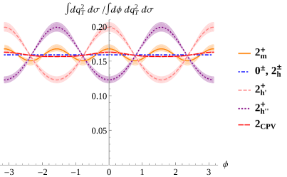
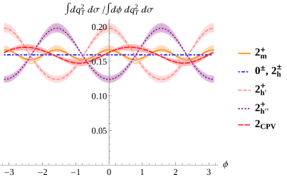
Figure 1: Plot of the CS $\phi$ distribution in the process $pp\to X_{i}X\to\gamma\gamma X$ for a 125 GeV resonance $X_{i}$ at a center of mass energy of 8 TeV, for various $X_{i}$ coupling scenarios at $\theta=\pi/2$ and at $Y=0$ (left) and $Y=1$ (right). The upper limit on the $q_{\scriptscriptstyle T}$ integration has been chosen as $M_{h}/2$. The shaded area is due to the uncertainty in the degree of polarization.

In Figure 1 we show our prediction for the CS $\phi$ distribution for central and forward Higgs production. The backward distribution can be obtained from the forward one by replacing $\phi\to-\phi$. From the plot we can see that various spin-2 coupling scenarios produce non-isotropic $\phi$ distributions. The difference from the isotropic spin-0 distribution is of such a size that, with the given collected data set, it might well be possible to put constraints on various spin-2 coupling hypotheses. Especially the benchmark scenarios $2_{h^{\prime}}$ and $2_{h^{\prime\prime}}$ are significantly different from the spin-0 scenario and could therefore relatively easily be excluded. The $2_{\text{CPV}}$ benchmark scenario displays a characteristic asymmetric $\phi$ distribution in the forward region that can only be caused by a $CP$-violating coupling.

Conclusion

We have presented the CS angle $\phi$ distribution in the process $pp\to X_{i}X\to\gamma\gamma X$, for $X_{i}$ a spin-0 and spin-2 boson with generic couplings, taking into account the fact that gluons inside an unpolarized proton are partially linearly polarized. Numerical predictions of the $\phi$ distribution show that various spin-2 coupling scenarios differ substantially from the isotropic spin-0 prediction, to an extent that a measurement of this distribution, based on the current data set collected by ATLAS and CMS, might already be enough to exclude these scenarios.

References

• [1] G. Aad et al. [ATLAS Collaboration], Phys. Lett. B 716, 1 (2012)
• [2] S. Chatrchyan et al. [CMS Collaboration], Phys. Lett. B 716, 30 (2012)
• [3] G. Aad et al. [ATLAS Collaboration], Phys. Lett. B 726, 120 (2013)
• [4] S. Chatrchyan et al. [CMS Collaboration], Phys. Rev. Lett.  110, 081803 (2013)
• [5] [ATLAS Collaboration], ATLAS-CONF-2013-040, ATLAS-CONF-2013-029.
• [6] [CMS Collaboration], CMS-PAS-HIG-13-005, CMS-PAS-HIG-13-016.
• [7] S. Y. Choi, D. J. Miller, 2, M. M. Muhlleitner and P. M. Zerwas, Phys. Lett. B 553, 61 (2003)
• [8] Y. Gao, A. V. Gritsan, Z. Guo, K. Melnikov, M. Schulze and N. V. Tran, Phys. Rev. D 81, 075022 (2010)
• [9] S. Bolognesi et al. Phys. Rev. D 86, 095031 (2012)
• [10] S. Y. Choi, M. M. Muhlleitner and P. M. Zerwas, Phys. Lett. B 718, 1031 (2013)
• [11] J. Ellis, R. Fok, D. S. Hwang, V. Sanz and T. You, Eur. Phys. J. C 73, 2488 (2013)
• [12] D. Boer, W. J. den Dunnen, C. Pisano, M. Schlegel and W. Vogelsang, Phys. Rev. Lett.  108, 032002 (2012)
• [13] W. J. den Dunnen, D. Boer, C. Pisano, M. Schlegel and W. Vogelsang, arXiv:1205.6931 [hep-ph].
• [14] D. Boer, W. J. den Dunnen, C. Pisano and M. Schlegel, Phys. Rev. Lett.  111, 032002 (2013)
• [15] X. -d. Ji, J. -P. Ma and F. Yuan, JHEP 0507, 020 (2005)
• [16] P. Sun, B. -W. Xiao and F. Yuan, Phys. Rev. D 84, 094005 (2011)
• [17] J. P. Ma, J. X. Wang and S. Zhao, Phys. Rev. D 88, 014027 (2013)
• [18] P. J. Mulders and J. Rodrigues, Phys. Rev. D 63, 094021 (2001)
• [19] J. -W. Qiu, M. Schlegel and W. Vogelsang, Phys. Rev. Lett.  107, 062001 (2011)
• [20] J. C. Collins and D. E. Soper, Phys. Rev. D 16, 2219 (1977).
• [21] L. D. Landau, Dokl. Akad. Nauk Ser. Fiz.  60, 207 (1948).
• [22] C. -N. Yang, Phys. Rev.  77, 242 (1950).
• [23] W. J. den Dunnen and M. Schlegel, arXiv:1310.4965 [hep-ph].