High order structure preserving explicit methods for solving linear-quadratic optimal control problems and differential games

Abstract

We present high order explicit geometric integrators to solve linear-quadratic optimal control problems and $N$-player differential games. These problems are described by a system coupled non-linear differential equations with boundary conditions. We propose first to integrate backward in time the non-autonomous matrix Riccati differential equations and next to integrate forward in time the coupled system of equations for the Riccati and the state vector. This can be achieved by using appropriate splitting methods, which we show they preserve most qualitative properties of the exact solution. Since the coupled system of equations is usually explicitly time dependent, a preliminary analysis has to be considered. We consider the time as two new coordinates, and this allows us to integrate the whole system forward in time using splitting methods while preserving the most relevant qualitative structure of the exact solution. If the system is a perturbation of an exactly solvable problem, the performance of the splitting methods considerably improves. Some numerical examples are also considered which show the performance of the proposed methods.

1 Introduction

Linear-quadratic (LQ) optimal control problems appear in many different fields in engineering abou03mre ; anderson90ocl ; reid ; speyer10poo as well as in quantum mechanics palao02qcb ; peirce88oco ; zhu98arm (see also brif10coq and references therein). In general, LQ optimal control problems are described by coupled systems of nonlinear differential equations with boundary conditions. The particular algebraic structure of the equations makes that, in general, the solutions have some qualitative properties which are relevant for the theoretical study, and for this reason we consider its preservation by the numerical methods to be of great interest in order to get reliable and accurate results.

Numerical methods for solving non linear BVPs are usually more involved (and computationally more costly) than initial value problems IVPs ascher88nso ; keller76nso ; na79cmi . We consider the numerical integration of LQ optimal control problems with high order explicit and structure preserving methods, i.e. methods which preserve most qualitative properties of the problem. These methods are referred as structure preserving methods. The method are explicit and the algorithms can be used with variable step as well as variable order, and they have a simple way to estimate the accuracy of the method.

The main idea is that, once the problem is reformulated as an IVP, to split the vector field into parts which are exactly solvable and such that each part preserves the desired structure of the solution. Then, high order splitting methods can be used. If the problem is explicitly time dependent or it can be considered as a small perturbation of an exactly solvable problem, the correct split and the splitting methods to be used require a more careful analysis. These methods can also be considered as exponential methods which have shown a high performance for linear problems blanes09tme ; blanes02hoo ; iser ; iserles99ots , and are usually referred as geometric numerical integrators.

The methods proposed are also adjusted for solving linear-quadratic $N$-player differential games (which have been extensively studied from the theoretical point of view anderson90ocl ; ba95 ; Cr71 ; engw ; SH69 ) since they can be considered as optimal linear control problems.

The paper is organized as follows. In Section 2 we introduce the equations to be solved in a LQ optimal control problem and present the non-linear matrix Riccati equation as an equivalent linear system of equations. In Section 3 we formulate the problem as an IVP with a previous backward time integration of the Riccati equation, we present a brief introduction to splitting methods and we show how these methods can be used on autonomous and non-autonomous problems. The case of perturbed systems is and the preservation of some qualitative properties by splitting methods is also considered. Section 4 considers the generalization to the numerical integration of differential games, and Section 5 is devoted to numerical experiments to illustrate the performance of the methods. Finally, Section 6 gives the conclusions of the work.

2 LQ optimal control problems

Let us consider the LQ optimal control problem

$$x^{\prime}=A(t)x+B(t)u(t),\quad\ \ x(0)=x_{0}\,,\quad\ \ 0=t_{0}\leq t\leq t_{f}=T\,,$$ (1)

where the unknown $x(t)\in\mathbb{R}^{n}$ is the dynamic state. Here $A(t)\in\mathbb{R}^{n\times n}\,$, $B(t)\in\mathbb{R}^{n\times r}$, and $\ u(t)\in\mathbb{R}^{r}$ is the control.

We consider a quadratic cost function given by

$$J=x^{T}(T)\,Q_{T}\,x(T)+\int_{0}^{T}\left\{x^{T}(t)Q(t)x(t)+u^{T}(t)R(t)u(t)\right\}dt\,,$$

where $Q(t),Q_{T}\in\mathbb{R}^{n\times n}$, are symmetric non-negative matrices, $R(t)\in\mathbb{R}^{r\times r}$ is symmetric and positive definite (i.e. $Q(t),Q_{T}\geq 0,\ R>0$) and $z^{T}$ denotes the transpose of $z$. It is well known that the optimal control is reached when $u$ is written as abou03mre ; anderson90ocl ; speyer10poo

$$u(t)\,=\,-\,R^{-1}(t)\,B^{T}(t)\,P(t)\,x(t)\,,$$ (2)

with $\,P(t)\in\mathbb{R}^{n\times n}\,$ satisfying the matrix Riccati differential equation (RDEs) with final conditions

$$P^{\prime}=-Q(t)-A^{T}(t)P-PA(t)+PS(t)P,\qquad P(T)=Q_{T},$$ (3)

wherein

$$S(t)\,=\,B(t)\,R^{-1}(t)\,B^{T}(t)\,,$$ (4)

is a symmetric $n\times n$ matrix and $S(t)\geq 0$. It is known that $P(t)$ is also a symmetric and non-negative matrix. Substituting (2) into (1) we have that

$$x^{\prime}=\Big{(}A(t)-S(t)P(t)\Big{)}x,\quad\ \ x(0)=x_{0}\,.$$ (5)

Notice that the product $S(t)P(t)$ is a non-negative matrix and the preservation of this property by numerical methods is important to stabilize the evolution of the state vector.

The goal is to compute $u(t)$ to be used to control the system, and this requires to numerically solve the coupled system of non linear differential equations with boundary conditions (3) and (5). The numerical solution of non linear BVPs is usually very involved, with computationally costly methods and significant storage requirements (one has to numerically integrate backward in time some of the equations, to store intermediate results and to make a forward integration using the stored results, or to use shooting methods ascher88nso ; na79cmi ).

We present a new algorithm which solves the problem as an IVP and then it allows to use variable step and variable order methods while preserving the geometric structure of the problem. In addition, the methods need low storage requirements and allows an immediate evaluation of the controls along the integration, being of great interest for real time control problems.

To this purpose it is useful to write the non-linear matrix RDE as an equivalent linear differential equation.

2.1 The matrix Riccati differential equation

For solving the RDE (3), it is usual to consider the following decomposition $PU=V$, with $U(t),V(t)\in\mathbb{R}^{n\times n}$. Let us denote

$$y(t)=\left[\begin{array}[]{c}U\\ V\end{array}\right];\quad K(t)=\left[\begin{array}[]{ccc}A(t)&-S(t)\\ -Q(t)&-A^{T}(t)\end{array}\right],$$

where $y(t)\in\mathbb{R}^{2n\times n},\ K(t)\in\mathbb{R}^{2n\times 2n}$, $S(t)$ is given by (4), and the matrices $A(t)$ and $Q(t)$, are given by (1) and (2), respectively. Then, it is easy to check that $y(t)$ is the solution of the IVP

$$y^{\prime}(t)=K(t)\,y(t);\qquad\quad y(T)=\left[\begin{array}[]{c}U(T)\\ V(T)\end{array}\right]=\left[\begin{array}[]{c}I\\ Q_{T}\end{array}\right]\,,$$ (6)

with conditions at the end of the interval, to be integrated backward in time. By engw ; JP95 , if (6) has an appropriate solution with $U(t)$ non singular, the solution of (3) can be calculated by

$$P(t)\,=\,V(t)\,U(t)^{-1}\,.$$ (7)

Conditions under which $U^{-1}$ exists are known (see abou03mre ; JoPo and references therein). In this work we assume $U(t)$ is non-singular, otherwise $P(t)$ would be unbounded and the equation for the state vector would not be well defined.

3 Geometric integrators for solving LQ optimal control problems

The coupled system of equations to be solve is given by

$$\frac{d}{dt}\left[\begin{array}[]{c}U\\ V\end{array}\right] = \left[\begin{array}[]{ccc}A(t)&-S(t)\\ -Q(t)&-A^{T}(t)\end{array}\right]\left[\begin{array}[]{c}U\\ V\end{array}\right],\quad\quad\left[\begin{array}[]{c}U(T)\\ V(T)\end{array}\right]=\left[\begin{array}[]{c}I\\ Q_{T}\end{array}\right]$$ (18)

$$\frac{dx}{dt} = \Big{(}A(t)-S(t)\,V(t)\,U(t)^{-1}\,\Big{)}x,\qquad\ \ x(0)=x_{0}\,.$$ (19)

Since the equation (18) is independent of (19), we propose to integrate backward the RDE to get $U(t_{0}),V(t_{0})$ with sufficiently high accuracy. The method for this backward integration can take large steps without frequent outputs and no storage requirement are necessary. Different methods can be used, and the best choice can depend on each particular problem (i.e. if the equation is autonomous, or if it is non-autonomous but the time-dependent matrices have a smooth time variation, etc.).

Intermediate solutions are not needed in this preliminary integration so, we have much freedom on the choice of the numerical method for the backward integration. This allows a fast way to get the initial conditions, $U(t_{0}),V(t_{0})$, for the RDE. Next, we have to integrate forward in time the following IVP

$$\frac{d}{dt}\left[\begin{array}[]{c}U\\ V\end{array}\right] = \left[\begin{array}[]{ccc}A(t)&-S(t)\\ -Q(t)&-A^{T}(t)\end{array}\right]\left[\begin{array}[]{c}U\\ V\end{array}\right],\quad\quad\left[\begin{array}[]{c}U(t_{0})\\ V(t_{0})\end{array}\right]=\left[\begin{array}[]{c}U_{0}\\ V_{0}\end{array}\right]$$

$$\frac{dx}{dt} = \Big{(}A(t)+S(t)\,V(t)\,U(t)^{-1}\,\Big{)}x,\qquad\ \ x(0)=x_{0}\,$$

$$u(t) = -\,R^{-1}(t)\,B^{T}(t)\,V(t)\,U(t)^{-1}\,x(t)\,.$$

The linearized RDE and the equation for the state vector can be written in short as follows

$$\begin{array}[]{rcl}v^{\prime}&=&M(t)v\\ x^{\prime}&=&N(t,\hat{v})x\end{array}$$ (21)

with $v=[U^{T}\ V^{T}]^{T},\ \hat{v}=VU^{-1}=P$ and $M,N$ are matrices of appropriate dimensions. This system of equations is separable into insolvable parts and then splitting methods can be used in a simple way to solve this problem. These methods preserve most qualitative properties of the solutions. Let us briefly introduce the idea of splitting methods as well as the particular methods which will be used.

3.1 Splitting Methods

Let us consider the initial value problem

$$x^{\prime}=f(x),\qquad x_{0}=x(0)\in\mathbb{R}^{D}$$ (22)

with $f:\mathbb{R}^{D}\longrightarrow\mathbb{R}^{D}$ and solution $x(t)=\varphi_{t}(x_{0})$, and suppose that the vector field is separable

$$f(x)=f^{[a]}(x)+f^{[b]}(x),$$ (23)

in such a way that the equations

$$x^{\prime} = f^{[a]}(x),\qquad x(0)=x_{0}^{a},$$ (24)

$$x^{\prime} = f^{[b]}(x),\qquad x(0)=x_{0}^{b},$$ (25)

can be integrated exactly, with solutions $x(h)=\varphi_{h}^{[a]}(x_{0}^{a})$ and $x(h)=\varphi_{h}^{[b]}(x_{0}^{b})$, respectively, at $t=h$, the time step. It is well known that the composition, $\chi_{h}=\varphi^{[b]}_{h}\circ\varphi^{[a]}_{h}$, is a first order method and

$$\psi_{h}=\varphi^{[a]}_{h/2}\circ\varphi^{[b]}_{h}\circ\varphi^{[a]}_{h/2},$$ (26)

is a symmetric second order method. Higher order methods can be obtained by composition

$$\psi_{h}=\varphi^{[b]}_{b_{m}h}\circ\varphi^{[a]}_{a_{m}h}\circ\cdots\circ\varphi^{[a]}_{a_{2}h}\circ\varphi^{[b]}_{b_{1}h}\circ\varphi^{[a]}_{a_{1}h},$$ (27)

for appropriate choices of coefficients $a_{i},b_{i}$. For simplicity, we denote the composition as : $b_{m}\,a_{m}\,\ldots\,b_{1}\,a_{1}$. For example, an efficient fourth-order method is given by the following sequence blanes02psp

$$b_{7}\,a_{7}\,b_{6}\,a_{6}\,b_{5}\,a_{5}\,b_{4}\,a_{4}\,b_{3}\,a_{3}\,b_{2}\,a_{2}\,b_{1}\,a_{1}$$

with $a_{1}=0$ and the scheme is symmetric ($a_{8-i}=a_{i+1},\ b_{8-i}=b_{i},\ i=1,2,\ldots$) so, it can be written as follows

$$b_{1}\,a_{2}\,b_{2}\,a_{3}\,b_{3}\,a_{4}\,b_{4}\,a_{4}\,b_{3}\,a_{3}\,b_{2}\,a_{2}\,b_{1}$$ (28)

which is a 6-stage method. It has 6 coefficients $b_{i}$ and 7 coefficients $a_{i}$, but the last evaluation of one step can be reused in the first map in the following step, and it is not counted for the computational cost (it is called the First Same As Last (FSAL) property). A sixth-order method is given by the following 10-stage symmetric sequence

$$a_{1}\,b_{1}\,a_{2}\,b_{2}\,a_{3}\,b_{3}\,a_{4}\,b_{4}\,a_{5}\,b_{5}\,a_{6}\,b_{5}\,a_{4}\,b_{4}\,a_{4}\,b_{3}\,a_{3}\,b_{2}\,a_{2}\,b_{1}\,a_{1}.$$ (29)

The coefficients of both methods (taken from blanes02psp ) are collected in Table 1 for convenience of the reader.

Table 1: Coefficients for different splitting methods

Coefficients of the 6-stage 4th-order method (28) $b_{1}=0.0792036964311957$ $a_{2}=0.209515106613362$ $b_{2}=0.353172906049774$ $a_{3}=-0.143851773179818$ $b_{3}=-0.0420650803577195$ $a_{4}=1/2-(a_{2}+a_{3})$ $b_{4}=1-2(b_{1}+b_{2}+b_{3})$

Coefficients of the 10-stage 6th-order method (29) $a_{1}=0.0502627644003922$ $b_{1}=0.148816447901042$ $a_{2}=0.413514300428344$ $b_{2}=-0.132385865767784$ $a_{3}=0.0450798897943977$ $b_{3}=0.067307604692185$ $a_{4}=-0.188054853819569$ $b_{4}=0.432666402578175$ $a_{5}=0.541960678450780$ $b_{5}=1/2-(b_{1}+\ldots+b_{4})$ $a_{6}=1-2(a_{1}+\ldots+a_{5})$ Coefficients of the 2-stage (4,2) method (41) $\displaystyle a_{1}=\frac{3-\sqrt{3}}{6}$ $b_{1}=1/2$ $a_{2}=1-2a_{1}$ Coefficients of the 5-stage (8,4) method (42) $a_{1}=0.07534696026989288842$ $b_{1}=0.19022593937367661925$ $a_{2}=0.5179168546882567823$ $b_{2}=0.84652407044352625706$ $a_{3}=1/2-(a_{1}+a_{2})$ $b_{3}=1-2(b_{1}+b_{2})$

The splitting methods we have presented are valid for autonomous equations because the exact solution of the equation (22) can be written formally as the exponential a Lie operator, $\varphi_{t}=\exp\big{(}t\ L_{f}\big{)}$, with $L_{f}\equiv f\cdot\nabla$. The map $\varphi_{t}$ can be approximated by a composition of exponentials of Lie operators associated to the vector fields $f^{[a]}$ and $f^{[b]}$. If the problem is non-autonomous, as usually is the case for LQ optimal control problems, one can take the time as a new coordinate and transform the original non-autonomous equation into an autonomous one in an extended phase space. However, for our problem it is advantageous to consider the time not as one but as two independent coordinates, and this has to be combined with an appropriate splitting method. For this reason, we consider separately the autonomous from the non-autonomous LQ optimal control problem.

3.2 The autonomous case

If the system is autonomous, we can compute the solution of the RDE (18) at $t_{0}$ as follows.

$$\left[\begin{array}[]{c}U_{0}\\ V_{0}\end{array}\right]=\exp\left((t_{0}-T)\left[\begin{array}[]{ccc}A&-S\\ -Q&-A^{T}\end{array}\right]\right)\left[\begin{array}[]{c}U_{T}\\ V_{T}\end{array}\right],$$ (30)

which can be accurately computed, for example, by a scaling and squaring method almohy10cta ; moler03ndw i.e. if we take $K_{i}$ as an accurate approximation to the scaled exponential

$$K_{i}\simeq\exp\left(\frac{(t_{0}-T)}{2^{i}}\left[\begin{array}[]{ccc}A&-S\\ -Q&-A^{T}\end{array}\right]\right)$$ (31)

(here $K_{i}$ can be, for example, a diagonal Padé approximation or a Taylor approximation) then

$$\left[\begin{array}[]{c}U_{0}\\ V_{0}\end{array}\right]\simeq\underbrace{\left(\cdots\left(K_{i}\right)^{2}\cdots\right)^{2}}_{i-times}\left[\begin{array}[]{c}U_{T}\\ V_{T}\end{array}\right],$$ (32)

which provides an accurate approximation to $U_{0},V_{0}$ from $U_{T},V_{T}$ with no intermediate results. Next, one has to integrate forward in time the system (21) which takes the form:

$$\frac{d}{dt}\left[\begin{array}[]{c}v\\ x\end{array}\right]=\left[\begin{array}[]{c}Mv\\ N(\hat{v})x\end{array}\right]$$ (33)

which is separable into two solvable parts

$$\frac{d}{dt}\left[\begin{array}[]{c}v\\ x\end{array}\right]=\left[\begin{array}[]{c}Mv\\ 0\end{array}\right],\qquad\qquad\frac{d}{dt}\left[\begin{array}[]{c}v\\ x\end{array}\right]=\left[\begin{array}[]{c}0\\ N(\hat{v})x\end{array}\right].$$ (34)

The following algorithm can be used to advance one time step, $h$, from $t_{n}$ to $t_{n+1}=t_{n}+h$, by using an splitting method with coefficients $\{a_{i},b_{i}\}_{i=1}^{m}$

$$\begin{array}[]{l}(v^{0},x^{0})=(v_{n},x_{n})\\ {\bf do}\ \ i=1,\ldots,m\\ \quad{x}^{i}=\exp\left(a_{i}hN(\hat{v}^{i-1})\right)x^{i-1}\\ \quad{v}^{i}=\exp\left(b_{i}hM\right)v^{i-1}\\ {\bf enddo}\\ (v_{n+1},x_{n+1})=(v^{m},x^{m})\\ u_{n+1}=-\,R^{-1}\,B^{T}\,V_{n+1}\,U_{n+1}^{-1}\,x_{n+1}\,.\end{array}$$

In order to save computational cost, we can compute and store the following exponentials

$$E_{i}=\exp\left(b_{i}hM\right),\qquad i=1,2,\ldots,m.$$

To take advantage of the FSAL property to save the computation of a map, one has to slightly adjust the previous algorithm. Notice that this algorithm allows to compute the controls, $u_{n}$, jointly with the numerical solution of the equations and this can be convenient for real time experiments. Obviously, at $t=T$ we must reach the exact solution $P(T)=Q_{T}$ with accuracy up to round off accuracy.

3.3 The non-autonomous case

If the system is non-autonomous, the solution of the RDE has no analytic solution in a closed form. In this case we have to solve numerically the RDE backward in time using, for example, high order Magnus integrators (e.g. a method of order six or eight blanes02hoo ) which have shown a high performance while preserving most qualitative properties. Other methods like a high order extrapolation method can also be used. Once we have $U_{0},V_{0}$, we need to integrate forward in time the system of non autonomous equations. If we split the system as in the autonomous case, we end up with two non-autonomous problems, both with no solution in a closed form. We are then looking for an alternative split which provides the same accuracy while preserving the qualitative structure of the problem. This can be achieved by frozen the time following a proper sequence. To this purpose, we take the time not as a new coordinate, but as two new coordinates as follows

$$\left\{\begin{array}[]{rcl}\displaystyle v^{\prime}&=&M(t_{1})v\\ \displaystyle x^{\prime}&=&N(t_{2},\hat{v})x\\ \displaystyle t_{1}^{\prime}&=&1\\ \displaystyle t_{2}^{\prime}&=&1\end{array}\right.$$ (35)

where $\,{}^{\prime}\equiv\frac{d}{dt},\,$ and which we split as follows

$$\left\{\begin{array}[]{rcl}\displaystyle v^{\prime}&=&M(t_{1})v\\ \displaystyle x^{\prime}&=&0\\ \displaystyle t_{1}^{\prime}&=&0\\ \displaystyle t_{2}^{\prime}&=&1\end{array}\right.\qquad\qquad\left\{\begin{array}[]{rcl}\displaystyle v^{\prime}&=&0\\ \displaystyle x^{\prime}&=&N(t_{2},\hat{v})x\\ \displaystyle t_{1}^{\prime}&=&1\\ \displaystyle t_{2}^{\prime}&=&0\end{array}\right.$$ (36)

This corresponds to two linear autonomous equations in the extended phase space, and each part is now exactly solvable. Then, the same splitting methods as in the autonomous case can be used. The algorithm for one time step, $h$, is given by:

$$\begin{array}[]{l}(v^{0},x^{0},t_{1}^{0},t_{2}^{0})=(v_{n},x_{n},t_{n},t_{n})\\ {\bf do}\ \ i=1,m\\ \quad{x}^{i}=\exp\big{(}\,a_{i}hN(t_{1}^{i-1},\hat{v}^{i-1})\,\big{)}x^{i-1}\\ \quad t_{2}^{i}=t_{2}^{i-1}+a_{i}h\\ \quad{v}^{i}=\exp\big{(}\,b_{i}hM(t_{2}^{i})\,\big{)}v^{i-1}\\ \quad t_{1}^{i}=t_{1}^{i-1}+b_{i}h\\ {\bf enddo}\\ (v_{n+1},x_{n+1},t_{n+1},t_{n+1})=(v^{m},x^{m},t_{1}^{m},t_{2}^{m})\\ u_{n+1}=-\,R^{-1}(t_{n+1})\,B^{T}(t_{n+1})\,V_{n+1}\,U_{n+1}^{-1}\,x_{n+1}\,.\end{array}$$ (37)

Since the matrix $M(t)$ changes at each step, the exponentials, $\exp\big{(}b_{i}hM(t_{2}^{i})\big{)}$, need to be computed at each step. If this is the most time consuming part of the algorithm, it is possible to look for an algorithm in which the exponentials can be replaced by a much more economical symmetric second order approximation, as for example a second order diagonal Padé approximation

$$\Phi_{b_{i}h}^{[b]}(t_{2}^{i})=\frac{I+\frac{1}{2}b_{i}hM(t_{2}^{i})}{I-\frac{1}{2}b_{i}hM(t_{2}^{i})}=\exp(b_{i}hM(t_{2}^{i}))+\mathcal{O}(h^{3}).$$

In general, $M$ belongs to the Lie algebra of symplectic matrices and the exponential belongs to the associated symplectic Lie group. Diagonal Padé approximations preserve this group property for the symplectic algebra iser . Now it is important to keep in mind that one can not use the coefficients from Table 1 since they are designed for problems which are separable in two parts such that both are exactly solved.

We can proceed as follows. Let $S^{[2]}_{h}$ be the following symmetric second order method

$$S^{[2]}_{h}=\varphi^{[a]}_{h/2}\circ\Phi_{h}^{[b]}\circ\varphi^{[a]}_{h/2}:\left\{\begin{array}[]{l}\quad x^{1/2}=\exp\left(\frac{h}{2}N(t_{1}^{0},\hat{v}^{0})\right)x^{0}\\ \quad t_{2}^{1/2}=t_{2}^{0}+\frac{h}{2}\\ \quad v^{1}=\Phi^{[b]}_{h}(t_{2}^{1/2})v^{i-1}\\ \quad t_{1}^{1}=t_{1}^{0}+h\\ \quad x^{1}=\exp\left(\frac{h}{2}N(t_{1}^{1},\hat{v}^{1})\right)x^{1/2}\\ \quad t_{2}^{1}=t_{2}^{1/2}+\frac{h}{2}\\ \end{array}\right.$$ (38)

Taking $S^{[2]}_{h}$ as the basic method, we can build methods of order, $p$, with $p>2$, as a composition of this basic method

$$S^{[p]}_{h}=\prod_{i=1}^{m}S^{[2]}_{\alpha_{i}h}.$$ (39)

The following fourth-order method shows a good performance to get solutions up to relatively high accuracies (for methods built in this way)

$$S^{[4]}_{h}=S^{[2]}_{\alpha_{1}h}\circ S^{[2]}_{\alpha_{1}h}\circ S^{[2]}_{\alpha_{2}h}\circ S^{[2]}_{\alpha_{1}h}\circ S^{[2]}_{\alpha_{1}h}$$

with $\alpha_{1}=1/(4-4^{1/3}),\ \alpha_{2}=-4^{1/3}/(4-4^{1/3})$. Several sets of coefficients for methods of different orders and number of stages are collected in hairer06gni ; mclachlan02sm .

Notice that at $t=T$ we must reach a numerical approximation close to the exact solution $P(T)=Q_{T}$. The methods presented in this work will approximate this value with accuracy up to the order of the method, i.e. $P_{ap}(T)=Q_{T}+\mathcal{O}(h^{p})$, and this can be used as a measure of the accuracy of the algorithm.

3.4 Methods for near-integrable problems

In some cases, LQ optimal control problems can be formulated as a small perturbation of an exactly solvable problem (or which can be easily solved by a numerical method). In this case it can be convenient to split between the dominant part and the perturbation, and to use splitting methods designed for separable problems with this structure. Then, if we have the IVP

$$x^{\prime}=f^{[a]}(x)+\varepsilon f^{[b]}(x)$$ (40)

where $|\varepsilon|\ll 1$ and both equations are either exactly solvable or can be efficiently solved by a numerical method, splitting methods tailored for this problem usually have a very good performance. For example, two highly efficient methods are given by the following compositions and whose coefficients from mclachlan95cmi are collected in Table 1

$$a_{1}\,b_{1}\,a_{2}\,b_{1}\,a_{1}$$ (41)

which is referred as a (4,2) method (a second order methods which, in the limit $\varepsilon\rightarrow 0$, behaves as a fourth order method) and

$$a_{1}\,b_{1}\,a_{2}\,b_{2}\,a_{3}\,b_{3}\,a_{3}\,b_{2}\,a_{2}\,b_{1}\,a_{1}$$ (42)

which corresponds to a (8,4) method. More elaborated methods with more stages are given in blanes13nfo .

If the problem is non-autonomous

$$x^{\prime}=f^{[a]}(x,t)+\varepsilon f^{[b]}(x,t)$$ (43)

it is still possible to take the time as a new coordinate (only one new coordinate instead of two contrarily to the previous and more general case) and the structure of a near integrable problem remains, in the extended phase space, if we split the system as follows blanes10sac

$$\frac{d}{dt}\left[\begin{array}[]{c}x\\ t_{1}\end{array}\right]=\left[\begin{array}[]{c}f^{[a]}(x,t_{1})\\ 1\end{array}\right]+\varepsilon\left[\begin{array}[]{c}f^{[b]}(x,t_{1})\\ 0\end{array}\right].$$ (44)

If the time is considered as two different coordinates as in the general separable case, this structure of a perturbed problem is lost. This requires to integrate exactly or up to high accuracy the non-autonomous equation associated to the dominant part

$$x^{\prime}=f^{[a]}(x,t),$$ (45)

and to solve the perturbed part with the time frozen.

For example, LQ optimal control problems where the matrix $A$ is constant and $\|A\|\gg\|S\|$ and $\|A\|\gg\|Q\|$ have this structure. We can split the problem as follows

$$x^{\prime}=f^{[a]}(x,t)\ :\ \left\{\begin{array}[]{rcl}\left[\begin{array}[]{c}U\\ V\end{array}\right]^{\prime}&=&\left[\begin{array}[]{ccc}A&0\\ 0&-A^{T}\end{array}\right]\left[\begin{array}[]{c}U\\ V\end{array}\right],\\ x^{\prime}&=&\Big{(}A-S(t)\,V(t)\,U(t)^{-1}\,\Big{)}x\end{array}\right.$$ (46)

with solution for the matrix RDE: $U=e^{(t-t^{*})A}U^{*},\ V=e^{-(t-t^{*})A^{T}}V^{*}$, where $U^{*},\,V^{*}$ are the initial conditions at each stage at $t=t^{*}$. The equation for the state vector is then

$$x^{\prime}=\Big{(}A+S(t)\,e^{-(t-t^{*})A^{T}}V^{*}\,U^{*-1}e^{-(t-t^{*})A}\,\Big{)}x.$$

This is a linear equation of the form

$$x^{\prime}=M(t)x$$ (47)

which in general has no analytical solution in a closed form, but can be numerically solved to high accuracy by using, for example, a Magnus integrator blanes09tme . Notice that, for the numerical integration, the matrix $M(t)$ has to be evaluated on a number of quadrature nodes, $t_{i}=t^{*}+c_{i}h$, for a time step, $h$. Then, the exponentials $e^{-c_{i}hA}$ have to be evaluated only once at the nodes of the quadrature rule and can be used on each time step.

Magnus integrators are exponential integrators which preserve most qualitative properties of the exact solution. The methods are explicit and usually have similar stability properties than implicit methods because most implicit methods can be seen as rational approximations to the exponentials appearing in the Magnus integrators. Standard Magnus integrators blanes09tme involve commutators of the matrix $M(t)$ evaluated a different instants. Magnus integrators which do not involve commutators (commutator-free methods) also exist and in many cases are simpler to implement. For example, a fourth-order method for the integration from $t_{n}$ to $t_{n+1}=t_{n}+h$ is given by

$$x_{n+1}=\exp\left(\frac{h}{12}\left(-M_{0}+4M_{1/2}+3M_{1}\right)\right)\exp\left(\frac{h}{12}\left(3M_{0}+4M_{1/2}-M_{1}\right)\right)x_{n},$$

where $M_{i}=M(t_{n}+ih)$. High order commutator-free methods can be found in alvermann11hoc ; blanes06fas .

Next, the coordinate $t_{1}$ is advanced and for the perturbation we have to solve the autonomous problem ($x^{\prime}=\varepsilon f^{[b]}(x,t_{1})$)

$$\frac{d}{dt}\left[\begin{array}[]{c}U\\ V\end{array}\right] = \left[\begin{array}[]{ccc}0&-S(t_{1})\\ -Q(t_{1})&0\end{array}\right]\left[\begin{array}[]{c}U\\ V\end{array}\right],$$ (54)

where the value of $t_{1}$ is frozen. Since $\|Q\|$ and $\|S\|$ are small, it suffices, for most practical purposes, to approximate the exact solution by a low order Taylor method.

3.5 Structure preservation of the splitting methods

It is well known that given the autonomous matrix RDE

$$P^{\prime}=-Q-A^{T}P-PA+PSP,\qquad P(T)=Q_{T},$$ (55)

where $Q,S,Q_{T}$ are symmetric non negative matrices, the solution $P(t)$ is also a symmetric matrix and $P(t)\geq 0,\ t\in[0,T]$. The same result is also valid for the non-autonomous equation

$$P^{\prime}=-Q(t)-A^{T}(t)P-PA(t)+PS(t)P,\qquad P(T)=Q_{T},$$ (56)

if the time-dependent matrices $Q(t),A(t),S(t)$ are continuous, $Q(t),S(t)$ are symmetric and non negative for $t\in[0,T]$ and $Q_{T}$ is a symmetric non negative matrix.

This is a very important property because the matrix $P(t)$ is coupled with the equation for the state vector and plays an important role on its stability. Standard methods do not preserve the positivity property of the matrix $P$. However, some of the splitting methods we have presented in this work will preserve this property.

Notice that in the split (36) one freezes the time in the matrix RDE and solves exactly the corresponding autonomous equation

$$P^{\prime}=-Q(t_{1})-A^{T}(t_{1})P-PA(t_{1})+PS(t_{1})P,\qquad P(t^{*})=P^{*},$$ (57)

where $Q(t_{1}),S(t_{1})$ are symmetric non negative matrices. Then if $P^{*}$ is a symmetric non negative matrix the numerical solution $P_{ap}(t)$ is also a symmetric matrix and $P_{ap}(t)\geq 0,\ t\in[t^{*}-h,t^{*}]$.

Unfortunately, it is well known that splitting methods of order higher than two necessarily have at least one coefficient $a_{i}$ negative and at least one coefficient $b_{i}$ negative, and then splitting methods of order greater than two can not guarantee positivity (a similar result was obtained for the preservation of positivity of commutator-free methods studied in blanes12mif ). One expects, however, a better preservation of this property with respect to standard methods. In a splitting method we can choose either the coefficients $a_{i}$ or $b_{i}$ to advance the RDE. If positivity is an important property, it is convenient to advance the RDE with maps associated to the coefficients having the smaller negative value. For example, we have interchanged the coefficients $a_{i}$ and $b_{i}$ in the 6-stage fourth-order method (28) as given in blanes02psp so $\ \min\{b_{i}\}>\min\{a_{i}\}\$ because the RDE is advanced with the coefficients $b_{i}$ in the algorithm.

4 Differential games with $N$ players

Let us now consider the problem of differential games with $N$ players given by the equations

$$x^{\prime}(t)=A(t)x(t)+\sum_{i=1}^{N}B_{i}(t)u_{i}(t),\qquad x(0)=x_{0}\,,$$ (58)

and the quadratic cost function

$$J_{i}=x^{T}(T)\,Q_{iT}\,x(T)$$ (59)

$$+\int_{0}^{T}\left\{x^{T}(t)Q_{i}(t)x(t)+u_{i}^{T}(t)R_{ii}(t)u_{i}(t)+\sum_{j=1,j\neq i}^{N}u_{j}^{T}(t)R_{ij}(t)u_{j}(t)\right\}dt$$

$i=1,\ldots,N$. From SH69 , for a zero sum game it is necessary that $R_{ij}\neq 0$, $i\neq j$, but in a non-zero sum game it is natural to choose $R_{ij}=0$, $i\neq j$, because in the most frequent applications the cost function of each player does not contain the other player control. In this way, the quadratic cost function $J_{i}$ depends only on the control $u_{i}$.

Let us first consider a non-cooperative non-zero sum game where each player, in order to minimize their cost function, determines his action in an independent way knowing only the initial state of the game and the model structure. Under these conditions the optimal controls are given by

$$u_{i}(t)\,=\,-\,R_{ii}^{-1}(t)\,B_{i}^{T}(t)\,P_{i}(t)\,x(t)\,,\qquad i=1,\ldots,N,$$

where the matrices $P_{i}$, satisfy the coupled matrix RDEs

$$\begin{array}[]{c}P^{\prime}_{i}=-Q_{i}(t)-A^{T}(t)P_{i}-P_{i}A(t)+\sum_{j=1}^{N}P_{i}S_{j}(t)P_{j}\end{array}$$ (60)

with $S_{i}(t)=B_{i}(t)\,R_{ii}^{-1}(t)\,B_{i}^{T}(t)$, $i=1,\ldots,N$. If we denote by

$$W(t)=\left[\begin{array}[]{c}P_{1}(t)\\ \vdots\\ P_{N}(t)\end{array}\right]\in\mathbb{R}^{Nn\times n}\,,\qquad C(t)=\left[\begin{array}[]{c}-Q_{1}(t)\\ \vdots\\ -Q_{N}(t)\end{array}\right]\in\mathbb{R}^{Nn\times N}\,,$$ (61)

$$B(t)=\left[\,-S_{1}(t)\ \ \cdots\ \ -S_{N}(t)\,\right]\in\mathbb{R}^{n\times Nn}\,,$$ (62)

$$D(t)\,=\,\left[\begin{array}[]{cccc}A^{T}(t)&0&\cdots&0\\ 0&A^{T}(t)&\cdots&0\\ \vdots&\vdots&\ddots&\vdots\\ 0&0&\cdots&A^{T}(t)\end{array}\right]\in\mathbb{R}^{Nn\times Nn}\,,$$ (63)

then, the coupled system (60) can be written as

$$W^{\prime}(t)=C(t)-D(t)W(t)-W(t)A(t)-W(t)B(t)W(t)\,.$$

From JoPo ; reid , if we consider $\,y(t)\in\mathbb{R}^{(N+1)n\times n}\,$ the solution of the linear equation

$$y^{\prime}(t)\,=\,\left[\begin{array}[]{cr}A(t)&B(t)\\ C(t)&-D(t)\end{array}\right]\,y(t)\,;\quad\quad y(T)=\left[\begin{array}[]{c}U(T)\\ V_{1}(T)\\ \vdots\\ V_{N}(T)\end{array}\right]=\left[\begin{array}[]{c}I\\ Q_{1T}\\ \vdots\\ Q_{NT}\end{array}\right]\,,$$ (64)

where $Z=[V_{1}^{T},\ldots,V_{N}^{T}]^{T}$ and $Z_{T}=[Q_{1T}^{T},\ldots,Q_{NT}^{T}]^{T}$,and we have that $P_{i}(t)\,=\,V_{i}(t)\,U(t)^{-1}.$

As in the previous case, we can integrate backward in time the coupled RDEs (64) with a highly accurate method. Once the initial conditions are obtained, we can integrate forward in time the whole systems, which provides us the numerical values of the controls along the time. The system to be solved is:

$$\frac{d}{dt}\left[\begin{array}[]{c}U\\ Z\end{array}\right] = \left[\begin{array}[]{ccc}A(t)&B(t)\\ -C(t)&-D(t)\end{array}\right]\left[\begin{array}[]{c}U\\ Z\end{array}\right],\quad\quad\left[\begin{array}[]{c}U(t_{0})\\ Z(t_{0})\end{array}\right]=\left[\begin{array}[]{c}U_{0}\\ Z_{0}\end{array}\right]$$ (75)

$$\frac{dx}{dt} = \Big{(}A(t)-\sum_{i=1}^{N}S_{i}(t)\,V_{i}(t)\,U(t)^{-1}\,\Big{)}x,\qquad\ \ x(0)=x_{0}\,$$ (76)

$$u_{i}(t) = -\,R_{ii}^{-1}(t)\,B_{i}^{T}(t)\,V_{i}(t)\,U(t)^{-1}\,x(t)\,.$$ (77)

This problem has formally the same structure as the LQ optimal control problem, and the numerical integration can be carried out using the same methods as previously. The main difference remains on the size of the matrices, and then its computational cost. For a large number of players it can be advantageous to consider approximations for the exponentials associated to the coupled RDEs.

4.1 Integrators for the zero sum game

From SH69 , for a zero sum game it is necessary that $R_{ij}\neq 0$, $i\neq j$. In this way, the quadratic cost functions $J_{i}$ depend on all controls $u_{i}$, $i=1,\ldots,N\,$. For simplicity in the presentation, we consider the case of two players. The coupled Riccati differential equations to be solved are

$$\begin{array}[]{rcl}P^{\prime}_{1}&=&-Q_{1}(t)-A^{T}(t)P_{1}-P_{1}A(t)+P_{1}S_{1}(t)P_{1}+P_{1}S_{2}(t)P_{2}+P_{2}S_{22}(t)P_{2}\,,\\ P^{\prime}_{2}&=&-Q_{2}(t)-A^{T}(t)P_{2}-P_{2}A(t)+P_{2}S_{2}(t)P_{2}+P_{2}S_{1}(t)P_{1}+P_{1}S_{11}(t)P_{1}\,,\end{array}$$

with the final conditions, $P_{1}(T)=Q_{1T}\,,\ \ P_{2}(T)=Q_{2T}\,,$ wherein

$$S_{ij}(t)\,=\,B_{i}(t)\,R_{ij}^{-1}(t)\,B_{i}^{T}(t)\,;\ \ i=1,\,2\,.$$

This problem can not be reformulated as a linear problem. This means we can not use exponential methods as previously. To integrate backward the coupled RDEs we can use a highly accurate method to avoid the loss in the preservation of the qualitative properties. A high order extrapolation method based on a symmetric second order integrator, say $\Phi_{h}^{[b]}$, would be a good choice. Then, this symmetric second order method can be used as the map in the composition (38) for the forward time integration, and we can use the composition methods given in (39).

5 Numerical examples

In order to test the performance of the numerical methods presented in this work we consider the problem of air pollutant emissions studied in kata and we have generalized this problem to the case of $N$ regions ($N$ players) and the constant parameters are replaced by time dependent functions

$$x^{\prime}=-a(t)x+b(t)\sum_{i=1}^{N}u_{i}(t);\qquad x(0)=x_{0}.$$ (78)

Here $x(t)\in\mathbb{R}$ is the excess of the pollutant in the atmosphere, $u_{i}(t)\in\mathbb{R}$, $i=1,\ldots,N$, denote the emissions of each region and $a(t)$, $b(t)$ are positive functions related with the intervention of the nature on environment. The cost functions to minimize is given by

$$J_{i}=\int_{0}^{T}e^{-\rho t}\left\{c_{i}(t)u_{i}^{2}(t)+d_{i}(t)x^{2}(t)\right\}\,dt\,,\ \ i=1,\ldots,N\,,$$ (79)

where $c_{i}(t)$, $d_{i}(t)$, are positive functions related to the costs of emission and pollution withstand respectively, and $\rho$ is a refresh rate. With an appropriate change of constants, the problem (78)-(79) can be applied to other situations, such as financial problems.

In our notation, $R_{ij}=0$, $i\neq j$, $Q_{iT}=0$, $Q_{i}(t)=d_{i}(t)e^{-\rho t}$, $R_{ii}=c_{i}(t)e^{-\rho t}$, and $S_{i}=b(t)^{2}e^{\rho t}/c_{i}(t)$, $i=1,\ldots,N$.

Then, we have:

• the equation (64) with the data

  $$y^{\prime}(t)=K(t)y(t)\,,\ \qquad y(T)=\left[1,\,0,\,\ldots\,,0\right]^{T}\,;$$

  $$y(t)=\left[\begin{array}[]{c}u(t)\\ v_{1}(t)\\ \vdots\\ v_{N}(t)\end{array}\right]\,;\ \ K(t)=\left[\begin{array}[]{cccc}-a(t)&-\displaystyle\frac{b(t)^{2}}{c_{1}(t)}e^{\rho t}&\cdots&-\displaystyle\frac{b(t)^{2}}{c_{N}(t)}e^{\rho t}\\ -d_{1}(t)e^{-\rho t}&a(t)&\cdots&0\\ \vdots&\vdots&\ddots&\vdots\\ -d_{N}(t)e^{-\rho t}&0&\cdots&a(t)\end{array}\right]\,,$$ (80)

  that must be solved from $t=T$ to $t=0$.

• To integrate forward in time the IVP

  $$y^{\prime}(t) = K(t)y(t)\,,\ \qquad y(0)=y_{0}\,,$$ (81)

  $$x^{\prime} = \left(-a(t)-b(t)^{2}e^{\rho t}\sum_{i=1}^{N}\frac{1}{c_{i}(t)}\,\frac{v_{i}(t)}{u(t)}\right)x\,,\ \ x(0)=x_{0}\,,$$ (82)

  $$u_{i}(t) = -\,\frac{1}{c_{i}(t)}\,e^{\rho t}\,b(t)\,\frac{v_{i}(t)}{u(t)}\,x(t)\,,\qquad\ i=1,\ldots,N.$$ (83)

In our numerical experiments we take $T=1$, initial conditions, $x_{0}=10$ and consider the case of $N=10$ players, and we will take different choices for the functions and parameters in order to analyze the performance of the methods on different conditions.

The new methods, denoted by SP$n$, where $n$ is the order of the method for the methods given in Table 1, will be tested versus the following standard numerical methods:

• RK4: The well known 4-stage fourth-order Runge-Kutta method.

• ODE45: The variable step and variable order algorithm ode45 implemented in Matlab.

• ODE113: The variable step and variable order algorithm ode113 implemented in Matlab.

We first consider the different cases for the autonomous problem and next we consider other cases in which different explicitly time-dependent functions are taken into account.

The autonomous problem

We first consider the case where the RDE is autonomous, which corresponds to the case $\rho=0$ and the functions $a,b,c_{i},d_{i}$ take constant values, so $K$ in (80) is a constant matrix and the solution to get the initial conditions $y(0)$ is given by

$$y(0)=e^{-TK}y(T).$$

The initial conditions for the matrix RDE is computed up to round off accuracy and the performance of the methods is measured by taking into account the forward time integration. The solution at $t=T$ satisfies that $u_{i}(T)=0,\ i=1,\ldots,N$, and this is exactly satisfied, up to round off error, by the splitting methods so we measure the error as $|x(T)-x_{ap}(T)|$, where $x_{ap}$ is the approximated solution obtained by the numerical integrators.

1. We first take the following values for the parameters:

   $$a=b=1,\qquad c_{i}=\frac{1}{d_{i}}=\frac{10+i}{2}.$$

   We measure the accuracy versus the number of function evaluations for each method when the numerical integration is carried out using different values of the time step (or different values for the absolute and relative tolerances for the methods ODE45 and ODE113. In the numerical experiments we consider AbsTol=$10^{-i}$, RelTol=$10^{1-i},\ i=0,1,2,\ldots$ For the splitting methods we measure the cost as the number of stages. Obviously, the splitting methods require the evaluation of several exponentials of matrices and the computational cost will depend on the problem. However, for the autonomous case most exponentials can be computed at the beginning and be stored to be used repeatedly along the integration.

   

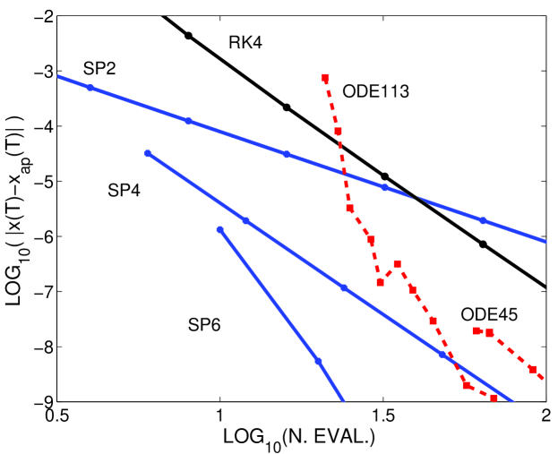
   Figure 1: Error $|x(T)-x_{ap}(T)|$ versus the number of evaluations for the autonomous case with 10 players and $a=b=1,\ c_{i}=1/d_{i}=(10+i)/2$.

   Figure 1 shows the results obtained. We observe that the splitting methods show more accurate results at the same number of evaluations. The performance of the new splitting methods could also be improved if the algorithms were implemented with variable order and variable step, as it is the case of ODE45 and ODE113.

2. We repeat the same experiment but for the case where

   $$a=2,\qquad b=1,\qquad c_{i}=\frac{1}{d_{i}}=\frac{100+i}{2}.$$

   This problem can be considered as a perturbed problem and we study the performance of the splitting methods (4,2) and (8,4) for the split given by (46) and (54), which are tailored for this class of problems.

   We solve separately the dominant part of the system, given by the equations

   $$\left[\begin{array}[]{c}u\\ v_{1}\\ \vdots\\ v_{N}\end{array}\right]^{\prime} = \left[\begin{array}[]{cccc}-2&0&\cdots&0\\ 0&2&\cdots&0\\ \vdots&\vdots&\ddots&\vdots\\ 0&0&\cdots&2\end{array}\right]\left[\begin{array}[]{c}u\\ v_{1}\\ \vdots\\ v_{N}\end{array}\right],\qquad\left[\begin{array}[]{c}u(t_{n})\\ v_{1}(t_{n})\\ \vdots\\ v_{N}(t_{n})\end{array}\right]=\left[\begin{array}[]{c}u_{n}\\ v_{1,n}\\ \vdots\\ v_{N,n}\end{array}\right]$$ (104)

   $$x^{\prime} = \left(-2-e^{\rho t}\sum_{i=1}^{N}\frac{1}{c_{i}}\,\frac{v_{i}(t)}{u(t)}\right)x\,,\qquad x(0)=x_{0}\,,$$ (105)

   where the RDE has trivial solution, which we plug into the equation of the state vector

   $$u(t) = e^{-2(t-t_{n})}u_{n}$$ (106)

   $$v_{i}(t) = e^{2(t-t_{n})}v_{i,n},\qquad i=1,\ldots,n$$ (107)

   $$x^{\prime} = \left(-2-e^{\rho t}e^{4(t-t_{n})}\sum_{i=1}^{N}\frac{1}{c_{i}}\,\frac{v_{i,n}}{u_{n}}\right)x\,.$$ (108)

   The equation for the state vector has exact solution since it is a scalar equation. In case it was a matrix equation, one could use, for example, a Magnus integrator, where the exponentials from the RDE can be computed for one time interval, and then used for all the integration. Figure 2 shows the results obtained. The schemes SP4 and SP6 lead to slightly worst results and are not showed.

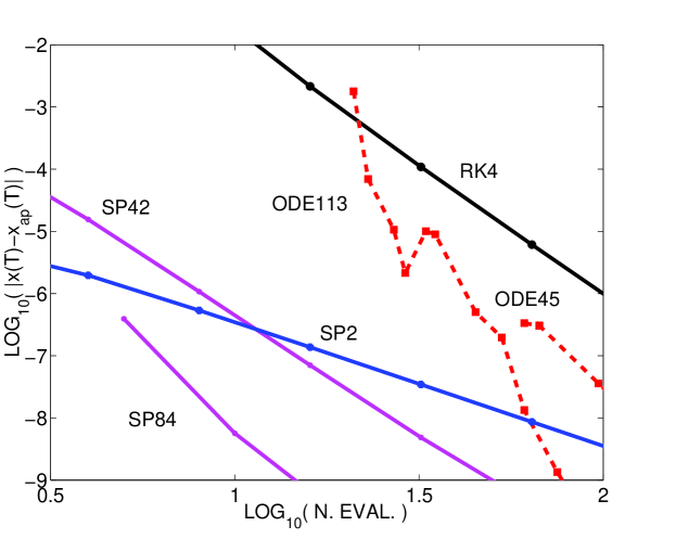
Figure 2: Error $|x(T)-x_{ap}(T)|$ versus the number of evaluations for the autonomous case with 10 players and $a=2,b=1,\ c_{i}=1/d_{i}=(100+i)/2$.

The non autonomous problem

We first consider the one player case, $N=1$, with the following choice for the functions and parameters

$$a(t)=2+\tanh\left(5(t-\frac{1}{2})\right),\quad\rho=\frac{1}{10},\quad b=1,\quad c_{1}=\frac{1}{d_{1}}=\frac{11}{2}.$$

where $a(t)\in[1,3]$, and we repeat the same experiments replacing the values of $c_{1},d_{1}$ by

$$c_{1}=\frac{1}{d_{1}}=\frac{101}{2}$$ (109)

which makes the system closer to a near integrable systems, in order to study the performance of the splitting methods in this case. We consider the split (36) and the algorithm (37). The case of one player corresponds to a LQ optimal control problem and, as already mentioned the solution of the RDE has to be a positive function. To show the superiority of the splitting methods when this property is important to be preserved, we measure the value of $P(T)=\frac{v(T)}{u(T)}$ for each method and choice of the time step. If this value is negative and smaller than a tolerance value, which we take $-10^{-8}$ (i.e. if $P_{ap}<-10^{-8}$) we marked this result with a circle.

Figure 3 illustrates the results obtained. The second order splitting methods preserves positivity for all time steps and the fourth- and sixth-order splitting methods do not preserve this property only for the largest time step, contrarily to the standard RK method or the methods implemented in Matlab. We observe that when the off diagonal coefficients of the RDE are small, the superiority of the splitting methods is even higher. We have repeated the numerical experiments with a higher number of players, and similar results are obtained.

Figure 3: Error $|x(T)-x_{ap}(T)|$ versus the number of evaluations for the autonomous case with 1 player and $a(t)=2+\tanh(5(t-1/2)),\ b=1,\ \rho=1/10$ and the following values for $c_{1},d_{1}$: Left panel $c_{1}=1/d_{1}=11/2$; right panel $c_{1}=1/d_{1}=101/2$. Solutions where $P_{ap}(T)<-10^{-8}\$ are marked with a circle.

6 Conclusions

We have considered the numerical integration of linear-quadratic optimal control problems and $N$-player differential games. These problems require to solve, backward in time, non-autonomous matrix Riccati differential equations which are coupled with the linear differential equations for the dynamic state. The solution of both problems allows to obtain the optimal control to be applied on the system in order to get the desired target. The system of equations which describe the problems have a particular algebraic structure which makes the solution to have some qualitative properties. We present high order explicit geometric integrators which preserve most qualitative properties. In particular, we analyze the positivity of the solution for the associated matrix Riccati differential equation, and we observe that the methods presented show a better preservation for this property. The coupled system of equations correspond to a non-linear boundary value problems which usually are solved by implicit and computationally very expensive algorithms. The methods proposed are explicit and are not iterative methods.

The methods proposed are high-order explicit geometric integrators which consider the time as two new coordinates. This allows us to integrate the whole system forward in time while preserving the most relevant qualitative structure of the exact solution. This allows an immediate evaluation of the control forward in time and then available for real time integrations. The numerical examples considered showed the performance of the proposed methods as well as the good preservation of some of the qualitative properties. Similar ideas could be used for solving non-linear optimal control problems after linearization blanes12mif , and using an iterative process, being this problem under consideration at this moment.

References

- (1) H. Abou-Kandil, G. Freiling, V. Ionescy and G. Jank, Matrix Riccati equations in control and systems theory. Burkhäuser Verlag, Basel. 2003.
- (2) Al-Mohy, A. H. and Higham, N. J. Computing the Action of the Matrix Exponential, with an Application to Exponential Integrators. SIAM J. Sci. Comp. 33, 488–511. 2011.
- (3) A. Alvermannand and H. Fehske, High-order commutator-free exponential time-propagation of driven quantum systems. J. Comput. Phys. 230, pp. 5930–5956. 2011.
- (4) B. D. O. Anderson and J. B. Moore, Optimal control: linear quadratic methods. Dover, New York. 1990.
- (5) Ascher, U. M., Mattheij, R. M. and Russell, R. D. Numerical solutions of boundary value problems for ordinary differential equations. Prentice-Hall. Englewood Cliffs, NJ. (1988).
- (6) P. Bader, S. Blanes, and E. Ponsoda, Structure preserving integrators for solving linear quadratic optimal control problems with applications to describe the flight of a quadrotor. Submitted. 2012.
- (7) T. Basar and G. J. Olsder, Dynamic non cooperative game theory, 2nd. Ed.. SIAM, Philadelphhia. 1999.
- (8) S. Blanes, F. Casas, A. Farrés, J. Laskar, J. Makazaga, and A. Murua, New families of symplectic splitting methods for numerical integration in dynamical astronomy. Appl. Numer. Math. 68 (2013), pp. 58-72.
- (9) S. Blanes, F. Casas, J. A. Oteo, and J. Ros, The Magnus expansion and some of its applications. Physics Reports, 470, pp. 151–238. 2009.
- (10) S. Blanes, F. Casas and J. Ros, High order optimized geometric integrators for linear differential equations. BIT, 42, pp. 262–284. 2002.
- (11) S. Blanes, F. Diele, C. Marangi, and S. Ragni, Splitting and composition methods for explicit time dependence in separable dynamical systems. J. Comput. Appl. Math., 235 (2010), pp. 646-659.
- (12) S. Blanes and P.C. Moan, Practical symplectic partitioned Runge-Kutta and Runge-Kutta-Nystr m methods, J. Comput. Appl. Math., 142 (2002), pp. 313-330.
- (13) S. Blanes and P.C. Moan, Fourth- and sixth-order commutator-free Magnus integrators for linear and non-linear dynamical systems, Appl. Num. Math., 56, pp. 1519-1537. 2006.
- (14) S. Blanes and E. Ponsoda, Magnus integrators for solving linear-quadratic differential games. J. Comput. Appl. Math. 236 (2012), pp. 3394-3408.
- (15) C. Brif, R. Chakrabarti, and H. Rabitz, Control of quantum phenomena: past, present and future. New J. Phys., 12, 075008 (68pp). 2010.
- (16) J. B. Cruz and C. I. Chen, Series Nash solution of two person non zero sum linear quadratic games. J. Optim. Theory Appl., 7, pp. 240-257. 1971.
- (17) J. Engwerda, LQ dynamic optimization and differential games. John Wiley and soons. 2005.
- (18) E. Hairer, C. Lubich and G. Wanner, Geometric Numerical Integration. Structure-Preserving Algorithms for Ordinary Differential Equations (2nd edition). Springer Series in Computational Mathematics, 31, Springer-Verlag, 2006.
- (19) A. Iserles, H. Z. Munthe-Kaas, S.P. Nørsett and A. Zanna, Lie group methods. Acta Numerica, 9, pp. 215–365. 2000.
- (20) A. Iserles and S. P. Nørsett, On the solution of linear differential equations in Lie groups. Philosophical Trans. Royal Soc., A 357,pp. 983–1019. 1999.
- (21) L. Jódar and E. Ponsoda, Non-autonomous Riccati-type matrix differential equations: existence interval, construction of continuous numerical solutions and error bounds. IMA J. Num. Anal., 15, pp. 61–74. 1995.
- (22) L. Jódar, E. Ponsoda and R. Company, Solutions of coupled Riccati equations arising in differential games. Control and Cybernetics, 24, No. 2, pp. 117–128. 1995.
- (23) V. Kaitala and M. Pohjola, Sustainable international agreement on greenhouse warming. A game theory study. Control and Game Theoretic Models of the Environment. Carraro and Filar Ed., Birkhauser, Boston, pp. 67–87. 1995.
- (24) H.B. Keller, Numerical solution of two point boundary value problems. CBMS-NSF Regional Conference Series in Applied Mathematics, 24, SIAM, Philadelphia. (1976).
- (25) R.I. McLachlan, Composition methods in the presence of small parameters, BIT 35 (1995), pp. 258 268.
- (26) R. I. McLachlan and, R. Quispel, Splitting Methods, Acta Numer., 11 (2002), pp. 341-434.
- (27) C. B. Moler and C. F. Van Loan, Nineteen Dubious Ways to Compute the Exponential of a Matrix, twenty-five years later. SIAM Review, 45, pp. 3–49. 2003.
- (28) Na, T.Y. Computational methods in engineering boundary value broblems. Mathematics in science and engineering, 145, Accademic Press, New York. (1979).
- (29) J.P. Palao and R. Kosloff, Quantum computing by an optimal control algorithm for unitry transformations. Phys. Rev. Lett., 28, 188304. 2002.
- (30) A.P. Peirce, M.A. Dahleh, and H. Rabitz, Optimal control of quantum-mechanical systems: existence, numerical approximation, and applications. Phys. Rev. A, 37, pp. 4950–4967. 1988.
- (31) W. T. Reid, Riccati Differential Equations. New York. Academic. 1972.
- (32) J.L. Speyer and D.H. Jacobson, Primer on optimal control theory. SIAM, Philadelphia, 2010.
- (33) A. W. Starr and Y. C. Ho, Non-zero sum differential games. J. Optim. Theory and Appl., 3, pp. 179–197. 1969.
- (34) W. Zhu and H. Rabitz, A rapid monotonically convergent iteration algorithm for quantum optimal control ever the expectation value of a positive definite operator, J. Chem. Phys. 109, pp. 385–391. 1998.