High-order splitting methods for separable non-autonomous parabolic equations

Abstract

We consider the numerical integration of non-autonomous separable parabolic equations using high order splitting methods with complex coefficients (methods with real coefficients of order greater than two necessarily have negative coefficients). We propose to consider a class of methods that allows us to evaluate all time-dependent operators at real values of the time, leading to schemes which are stable and simple to implement. If the system can be considered as the perturbation of an exactly solvable problem and the flow of the dominant part is advanced using real coefficients, it is possible to build highly efficient methods for these problems. We show the performance of this class of methods on several numerical examples and present some new improved schemes.

and  

1 Introduction

We consider the numerical integration of non-autonomous separable parabolic equations using high order splitting methods with complex coefficients. This class of methods has been recently used for the numerical integration of the autonomous case, showing good performances [5, 12, 17]. Splitting methods with real coefficients of order greater than two necessarily have negative coefficients and can not be used for solving these problems [4, 15, 21, 23]. However, solutions with complex coefficients with positive real part exist, and some of these methods can provide a high performance in spite the equations have to be solved in the complex domain. Previous works with applications among other in celestial mechanics and quantum mechanics where splitting methods with complex coefficients are considered already exist [2, 3, 13, 19, 20, 22, 23, 24].

A straightforward application of splitting methods with complex coefficients to non-autonomous problems require the evaluation of the time-dependent functions on the operators at complex times, and the corresponding flows in the numerical scheme are, in general, not well conditioned. In this work we propose to consider a class of splitting methods in which one set of the coefficients belong to the class of real and positive numbers. This can allow to evaluate all time-dependent operators at real values of the time, leading to schemes which are stable and simple to implement.

If the system can be considered as the perturbation of an exactly solvable problem (or easy to numerically solve) and the flow of the dominant part is advanced using the real coefficients, it is possible to build highly efficient methods for these problems.

1.1 The problem

Let us consider the non-autonomous separable PDE

$$\frac{du}{dt}={}A(t,u)+{}B(t,u),\qquad u(0)=u_{0},$$ (1.1)

$u(x,t)\in\mathbb{R}^{D}$, and where the (possibly unbounded) operators ${}A$, ${}B$ and ${}A+{}B$ generate $C^{0}$ semi-groups for positive $t$ over a finite or infinite Banach space. Equations of this form are encountered in the context of parabolic partial differential equations, an example being the inhomogeneous non-autonomous heat equation

$$\frac{\partial u}{\partial t}=\alpha(t)\Delta u+V(x,t)u,\quad\mbox{or}\quad\frac{\partial u}{\partial t}=\nabla(a(x,t)\nabla u)+V(x,t)u$$ (1.2)

where $t\geq 0$, $x\in\mathbb{R}^{d}$ or $x\in\mathbb{T}^{d}$ and $\Delta$ denotes the Laplacian with respect to the spatial coordinates, $x$. Another example corresponds to reaction-diffusion equations of the form

$$\frac{\partial u}{\partial t}=D(t)\Delta u+{}B(t,u),$$ (1.3)

where $D(t)$ is a matrix of diffusion coefficients (typically a diagonal matrix) and $B$ accounts for the reaction part. In general, $A(t,u),B(t,u)$ can also depend on $x,\nabla,$ etc., which are omitted for clarity in the presentation.

For simplicity, we write the non-linear equation (1.1) in the (apparently) linear form

$$\frac{du}{dt}=L_{A(t,u)}u+L_{B(t,u)}u,$$ (1.4)

where $L_{A},L_{B}$ are the Lie operators associated to ${}A,{}B$, i.e.

$$L_{A(t,u)}\equiv{}A(t,u)\frac{\partial}{\partial u},\qquad L_{B(t,u)}\equiv{}B(t,u)\frac{\partial}{\partial u}$$

which act on functions of $u$

If the problem is autonomous, the formal solution is given by $u(t)=\e^{t(L_{A(u)}+L_{B(u)})}u_{0}$, which is a short way to write

$$u(t)=\e^{t(L_{A(u)}+L_{B(u)})}u_{0}=\left.\sum_{k=0}^{\infty}\frac{t^{k}}{k!}\left({}A(u)\frac{\partial}{\partial u}+{}B(u)\frac{\partial}{\partial u}\right)^{k}u\ \right|_{u=u_{0}}.$$

If the subproblems

$$\frac{du}{dt}=A(u)\qquad\mbox{ and }\qquad\frac{du}{dt}=B(u)$$ (1.5)

have exact solutions or can efficiently be numerically solved, it is usual to consider splitting methods as numerical integrators. If we denote by $\e^{hL_{A(u)}},\ \e^{hL_{B(u)}}$ the exact $h$-flows for each problem in (1.5) (and for a sufficiently small time step, $h$) the simplest method within this class is the Lie-Trotter splitting

$$\e^{hL_{A(u)}}\,\e^{hL_{B(u)}}\qquad\mbox{ or }\qquad\e^{hL_{B(u)}}\,\e^{hL_{A(u)}},$$ (1.6)

which is a first order approximation in the time step to the solution, while the symmetrized version

$$S(h)=\e^{h/2\,L_{A(u)}}\,\e^{hL_{B(u)}}\,\e^{h/2\,L_{A(u)}}\qquad\mbox{ or }\qquad S(h)=\e^{h/2\,L_{B(u)}}\,\e^{hL_{A(u)}}\,\e^{h/2\,L_{B(u)}}$$ (1.7)

is referred to as Strang splitting, and is an approximation of order $2$, i.e. $S(h)=\e^{h(L_{A(u)+B(u)})}+\mathcal{O}(h^{3})$. Upon using an appropriate sequence of steps, high-order approximations can be obtained as

$$\Psi(h)=\e^{hb_{m+1}L_{B}}\,\e^{ha_{m}L_{A}}\,\cdots\,\e^{hb_{2}L_{B}}\,\e^{ha_{1}L_{A}}\,\e^{hb_{1}L_{B}},$$ (1.8)

and methods with real coefficients at any order can be obtained [14, 22, 26]. However, as already mentioned, splitting methods of order greater than two (with real coefficients) have at least one of the coefficients $a_{i}$ negative as well as at least one of the coefficients $b_{i}$ so, the flows $\e^{tL_{A}}$ and/or $\e^{tL_{B}}$ may not be well defined (this is indeed the case, for instance, for the Laplacian operator) and this prevents the use of methods which embed negative coefficients. For this reason, exponential splitting methods of at most order $p=2$ have been considered up to recently.

In order to circumvent this order-barrier, the papers [12] and [17] simultaneously presented a systematic analysis for a class of composition methods with complex coefficients having positive real parts. Using this extension from the real line to the complex plane, the authors of [12] and [17] built up methods of orders $3$ to $14$ by considering a technique known as triple-jump composition. More efficient high order methods are obtained in [5].

In this work we are interested, however, in the numerical integration of the non-autonomous problem (1.1) where the use of complex coefficients involve additional constraints as we will see. A method of choice for solving numerically (1.1) consists in advancing the solution alternatively along the exact (or numerical) solutions of the two problems

$$\frac{du}{dt}=A(t,u)\qquad\mbox{ and }\qquad\frac{du}{dt}=B(t,u).$$ (1.9)

The exact flows are, in general, not known. This is the case, for example, if $[L_{A(t_{i},u)},L_{A(t_{j},u)}]=L_{A(t_{i},u)}L_{A(t_{j},u)}-L_{A(t_{j},u)}L_{A(t_{i},u)}\neq 0$ (and similarly for $B(t)$). If the exact solution is not known, it can be replaced by a sufficiently accurate numerical approximation.

This procedure is equivalent to take the time as two new coordinates, $t_{1},t_{2}$

$$\left\{\begin{array}[]{l}u^{\prime}=A(t_{1},u)+B(t_{2},u)\\ t_{1}^{\prime}=1\\ t_{2}^{\prime}=1,\end{array}\right.$$ (1.10)

with ${}^{\prime}\equiv\frac{d}{dt}$, and to split the system in the extended space as follows [8]

$$\left\{\begin{array}[]{l}u^{\prime}=A(t_{1},u)\\ t_{1}^{\prime}=1\\ t_{2}^{\prime}=0\end{array}\right.\qquad\mbox{ and }\qquad\left\{\begin{array}[]{l}u^{\prime}=B(t_{2},u)\\ t_{1}^{\prime}=0\\ t_{2}^{\prime}=1.\end{array}\right.$$ (1.11)

A more convenient way to split the system which transforms the non-autonomous problems into autonomous is the following

$$\left\{\begin{array}[]{l}u^{\prime}=A(t_{1},u)\\ t_{1}^{\prime}=0\\ t_{2}^{\prime}=1\end{array}\right.\qquad\mbox{ and }\qquad\left\{\begin{array}[]{l}u^{\prime}=B(t_{2},u)\\ t_{1}^{\prime}=1\\ t_{2}^{\prime}=0.\end{array}\right.$$ (1.12)

Notice that the explicit time-dependency in $A$ and $B$ is frozen in each subproblem and the formal solution corresponds to the exponential of the Lie operators where the time dependency in the operators are frozen on each time interval. Unfortunately, to use splitting methods with complex coefficients for non-autonomous problems requires, in general, to compute $A(t,u),B(t,u)$ for $t\in\mathbb{C}$, leading, in general, to badly conditioned algorithms.

In this work we show that splitting method having one set of coefficients real and positive valued, i.e.

$$a_{i}\in\mathbb{R}^{+},\qquad b_{i}\in\mathbb{C}^{+},\qquad(\mbox{or}\quad a_{i}\in\mathbb{C}^{+},\qquad b_{i}\in\mathbb{R}^{+}),$$

allow to build algorithms where the operators $A(t,u),B(t,u)$ are evaluated only for $t\in\mathbb{R}$, leading to well defined methods. Several splitting methods with this structure have already been constructed.

We will also explore the case in which $\|B\|\ll\|A\|$, which we refer as a perturbed problem. We first show how this class of methods has to be used in these problems and next we study how to build high order efficient methods for these problems.

2 Splitting methods for non-autonomous problems

Suppose we have a splitting method with say, $a_{i}\in\mathbb{R}^{+}$ and $b_{i}\in\mathbb{C}^{+}$. To solve the eq. (1.9) we propose to take the time as one new coordinate and split the system as follows [8]

$$\left\{\begin{array}[]{l}u^{\prime}=A(t_{1},u)\\ t_{1}^{\prime}=1\end{array}\right.\qquad\mbox{ and }\qquad\left\{\begin{array}[]{l}u^{\prime}=B(t_{1},u)\\ t_{1}^{\prime}=0.\end{array}\right.$$ (2.1)

Let us denote by $\Phi_{A}^{[a_{i}h]}$ the map associated to the exact solution (or a sufficiently accurate numerical approximation) of the non-autonomous equation

$$\frac{du}{dt}={}A(t,u),\qquad\quad t\in[t_{n}+c_{i-1}h,t_{n}+c_{i}h]$$

with

$$c_{i}=\sum_{j=0}^{i}a_{j},$$

and $a_{0}=0$. Then, the splitting method (1.8) for the non-autonomous equation reads now

$$\Psi(h)=\e^{hb_{m+1}L_{B_{m}}}\,\Phi_{A}^{[a_{m}h]}\,\cdots\,\e^{hb_{2}L_{B_{1}}}\,\Phi_{A}^{[a_{1}h]}\,\e^{hb_{1}L_{B_{0}}},$$ (2.2)

where $B_{i}=B(t_{n}+c_{i}h,u).$ Notice that in this scheme, since $t_{1}$ is advanced with the coefficients $a_{i}$ (and then it takes real values) the operators $A(t,u)$ and $B(t,u)$ are evaluated on real values of $t$. On the other hand, if $A(t,u)$ is an unbounded operator and a numerical methods is used to approximate the flow $\Phi_{A}^{[h]}$, it must be well defined for $0\leq h<h^{*}$ for some positive $h^{*}$, and this is not guaranteed for general methods. For example, some commutator-free methods up to fourth-order can be used. Given the equation

$$\frac{du}{dt}=A(t,u),\qquad\qquad t\in[0,h]$$

we have that

$$\Phi_{A}^{[h]}=\e^{hL_{A(t_{n}+h/2,u)}}$$

corresponds to a symmetric second order method, and

$$\Phi_{A}^{[h]} = \e^{\frac{h}{2}(\alpha L_{A_{1}}+\beta L_{A_{2}})}\,\e^{\frac{h}{2}(\beta L_{A_{1}(u)}+\alpha L_{A_{2}(u)})}$$ (2.3)

$$= \Phi_{\frac{1}{2}(\beta A_{1}(u)+\alpha A_{2}(u))}^{[h]}\circ\Phi_{\frac{1}{2}(\alpha A_{1}(u)+\beta A_{2}(u))}^{[h]}$$

with $\alpha=\frac{1}{2}-\frac{\sqrt{3}}{3},\ \beta=1-\alpha$ and $A_{1}(u)=A\left(t_{n}+\left(\frac{1}{2}-\frac{\sqrt{3}}{6}\right)h,u\right),\ A_{2}(u)=A\left(t_{n}+\left(\frac{1}{2}+\frac{\sqrt{3}}{6}\right)h,u\right)$, corresponds to a fourth-order method [10, 25]. Notice that the Lie operators, since being derivatives, are written in the reverse order than the maps, and this is very important to keep inmind for non-linear non-autonomous problems in order to apply the method correctly (see [9] for more details on the Magnus series expansion and Magnus integrators for non-autonomous non-linear differential equations). This scheme corresponds to the composition of the 1-flow maps for the equations

$$u_{1}^{\prime} = \frac{h}{2}(\alpha A_{1}(u_{1})+\beta A_{2}(u_{1})),\qquad u_{1}(0)=u_{0}$$

$$u_{2}^{\prime} = \frac{h}{2}(\beta A_{1}(u_{2})+\alpha A_{2}(u_{2})),\qquad u_{2}(0)=u_{1}(1).$$ (2.4)

and the solution given by the map corresponds to $u_{2}(1)$. These second and fourth-order commutator-free methods can be used for unbounded operators and higher order commutator-free Magnus integrators for unbounded operators are under investigation at this moment [7].

2.1 Splitting methods for non-autonomous perturbed systems

In some cases, the system can be considered as the perturbation of an exactly solvable problem. In those cases, it is usually convenient to split into the dominant part and the perturbation and to build methods which take advantage of this relevant property. However, if the problem is non-autonomous and the time-dependency is not treated properly, the performance of the methods designed for perturbed problems deteriorate considerably.

Suppose that $\|B(t,u)\|\ll\|A(t,u)\|$. To make this fact more evident, we replace $B$ by $\varepsilon B$ with $|\varepsilon|\ll 1$. In the autonomous case, for example, the Lie-Trotter composition for this split satisfies

$$\e^{h(L_{A+\varepsilon B})}=\e^{h\,L_{A}}\e^{h\varepsilon L_{B}}+\frac{1}{2}\varepsilon h^{2}[L_{A},L_{B}]+\mathcal{O}(\varepsilon h^{3}),$$ (2.5)

i.e., it has a local error of order $\mathcal{O}(\varepsilon h^{2})$.

Since $A$ and $B$ are qualitatively different for perturbed problems, it is usual to consider $ABA$ and $BAB$ compositions.

An $m$-stage symmetric $BAB$ compositions given by

$$\Psi(h)=\e^{hb_{m+1}\varepsilon L_{B}}\,\e^{ha_{m}L_{A}}\,\cdots\,\e^{hb_{2}\varepsilon L_{B}}\,\e^{ha_{1}L_{A}}\,\e^{hb_{1}\varepsilon L_{B}},$$ (2.6)

with $a_{m+1-i}=a_{i},\ b_{m+2-1}=b_{i},\ i=1,2,\ldots$, and $ABA$ compositions are given by

$$\Psi(h)=\e^{ha_{m+1}L_{A}}\,\e^{hb_{m}\varepsilon L_{B}}\,\cdots\,\e^{ha_{2}L_{A}}\,\e^{hb_{1}\varepsilon L_{B}}\,\e^{ha_{1}L_{A}},$$ (2.7)

with $a_{m+2-i}=a_{i},\ b_{m+1-1}=b_{i},\ i=1,2,\ldots$. We will use the following short notation for these methods

$$(b_{m+1},a_{m},\,\cdots\,,b_{2},a_{1},b_{1})\qquad\mbox{and}\qquad(a_{m+1},b_{m},\,\cdots\,,a_{2},b_{1},a_{1}).$$

Notice that eq. (2.6) is a $BAB$ composition which, for the particular case where $b_{1}=b_{m+1}=0$ transforms into a $ABA$ composition (but with a different computational cost). It seems then natural to consider separately the following four cases:

1. $BAB:\quad a_{i}\in\mathbb{R}^{+},\quad b_{i}\in\mathbb{C}^{+}$,

2. $BAB:\quad a_{i}\in\mathbb{C}^{+},\quad b_{i}\in\mathbb{R}^{+}$,

3. $ABA:\quad a_{i}\in\mathbb{R}^{+},\quad b_{i}\in\mathbb{C}^{+}$,

4. $ABA:\quad a_{i}\in\mathbb{C}^{+},\quad b_{i}\in\mathbb{R}^{+}$.

The cases 2 and 4 require to split the system as follows

$$\left\{\begin{array}[]{l}u^{\prime}=A(t_{1},u)\\ t_{1}^{\prime}=0\end{array}\right.\qquad\mbox{ and }\qquad\left\{\begin{array}[]{l}u^{\prime}=\varepsilon B(t_{1},u)\\ t_{1}^{\prime}=1,\end{array}\right.$$ (2.8)

so $t_{1}$ will take real values. This split is similar to the one shown in the previous section by changing the roles of $A$ and $B$.

In the extended phase space these two systems are equivalent to solve separately the following system written in terms of Lie operators

$$\frac{d}{dt}\left\{\begin{array}[]{l}u\\ t_{1}\end{array}\right\}=\underbrace{\left({}A(t_{1},u)\frac{\partial}{\partial u}+0\cdot\frac{\partial}{\partial t_{1}}\right)}_{\mathcal{A}}\left\{\begin{array}[]{l}u\\ t_{1}\end{array}\right\}$$ (2.9)

$$\frac{d}{dt}\left\{\begin{array}[]{l}u\\ t_{1}\end{array}\right\}=\underbrace{\left(\varepsilon{}B(t_{1},u)\frac{\partial}{\partial u}+1\cdot\frac{\partial}{\partial t_{1}}\right)}_{\mathcal{B}}\left\{\begin{array}[]{l}u\\ t_{1}\end{array}\right\}.$$ (2.10)

The commutators of the Lie operators ${\mathcal{A}}$ and ${\mathcal{B}}$, which measure the error of the splitting methods in the extended phase space is

$$[h{\mathcal{A}},h{\mathcal{B}}]=h^{2}\big{(}{\mathcal{A}}{\mathcal{B}}-{\mathcal{B}}{\mathcal{A}}\big{)}=h^{2}\left(\varepsilon[{}A,{}B]-\frac{d{}A(t_{1},u)}{dt_{1}}\right)\frac{\partial}{\partial u}=\mathcal{O}(h^{2})$$

which is not proportional to $\varepsilon$ due to the term $\frac{dA(t_{1},u)}{dt_{1}}$, and this also happens with higher order commutators.

The cases 1 and 3 are associated to the split

$$\left\{\begin{array}[]{l}u^{\prime}=A(t_{1},u)\\ t_{1}^{\prime}=1\end{array}\right.\qquad\mbox{ and }\qquad\left\{\begin{array}[]{l}u^{\prime}=\varepsilon B(t_{1},u)\\ t_{1}^{\prime}=0.\end{array}\right.$$ (2.11)

This system can be written in the extended phase space as

$$\frac{d}{dt}\left\{\begin{array}[]{l}u\\ t_{1}\end{array}\right\}=\underbrace{\left({}A(t_{1},u)\frac{\partial}{\partial u}+1\cdot\frac{\partial}{\partial t_{1}}\right)}_{\mathcal{A}}\left\{\begin{array}[]{l}u\\ t_{1}\end{array}\right\}$$ (2.12)

$$\frac{d}{dt}\left\{\begin{array}[]{l}u\\ t_{1}\end{array}\right\}=\underbrace{\left(\varepsilon{}B(t_{1},u)\frac{\partial}{\partial u}+0\cdot\frac{\partial}{\partial t_{1}}\right)}_{\mathcal{B}}\left\{\begin{array}[]{l}u\\ t_{1}\end{array}\right\}$$ (2.13)

where now

$$[h{\mathcal{A}},h{\mathcal{B}}]=\varepsilon h^{2}\left([{}A,{}B]+\frac{dB(t_{1},u)}{dt_{1}}\right)\frac{\partial}{\partial u}=\mathcal{O}(\varepsilon h^{2})$$

which is proportional to the small parameter $\varepsilon$ (see [8] for more details).

Obviously, this split makes sense if one can exactly solve the non-autonomous equation associated to the dominant part

$$\frac{du}{dt}=A(t,u)$$ (2.14)

at a relatively low computational cost (or one can numerically solve it up to sufficiently high accuracy and at a relatively low computational cost) being the commutator-free Magnus integrators an appropriate choice in most cases. A similar methods was used in [1] for perturbed Schrödinger and Gross-Pitaevskii equations, but in those problems negative real coefficients are allowed.

2.2 Order conditions

For consistent symmetric methods we can formally write

$$\Psi(h) = \exp\left(h(L_{A}+\varepsilon L_{B})+h^{3}\,\left(\varepsilon\,p_{aba}[[L_{A},L_{B}],L_{A}]+\varepsilon^{2}\,p_{abb}[[L_{A},L_{B}],L_{B}])\right)\right.$$ (2.15)

$$\qquad\left.+h^{5}\left(\varepsilon\,p_{abaaa}[[[[L_{A},L_{B}],L_{A}],L_{A}],L_{A}]+\mathcal{O}(\varepsilon^{2})\right)+\mathcal{O}(\varepsilon h^{7})\right).$$

Following [6], for the composition (2.7) we have that (taking $m=s$)

$$p_{aba} \sim \frac{1}{2}\sum_{i=1}^{s}b_{i}c_{i}(1-c_{i})-\frac{1}{12},\qquad p_{abb}\sim\sum_{i=1}^{s}\frac{1}{2}b_{i}^{2}\,c_{i}+\sum_{1\leq i<j\leq s}b_{i}b_{j}c_{j}-\frac{1}{3},$$

$$p_{abaaa} \sim \sum_{i=1}^{s}b_{i}\,c_{i}^{4}-\frac{1}{5},$$ (2.16)

with $a_{0}=0$ and $c_{s+1}=1$. The symbol $\sim$ indicates that, if the low order conditions are satisfied, both terms are proportional so, if the r.h.s of $p_{aba}$ and $p_{abb}$ vanish then $p_{aba}=p_{abb}=0$. Here, the polynomial $p_{abaaa}$ corresponds to the dominant error term in fourth-order methods for perturbed problem. This algebraic analysis remains also valid for unbounded operators under appropriate conditions on the operators (see [16] for more details).

If we take $a_{1}=a_{m+1}=0$ we obtain a $BAB$ composition, and the equations of $p_{aba}$ and $p_{abb}$ can be easily adjusted to obtain $BAB$ compositions.

Second order symmetric methods which cancel the terms of order $h^{2p+1}\varepsilon$ for $p=1,2,\ldots,s$ and for different values of $s$ exist with positive and real coefficients [18]. The error of these methods is of order $\mathcal{O}(h^{2s+1}\varepsilon+h^{3}\varepsilon^{2})$ and we say the methods have effective order $(2s,2)$. For instance, a method which satisfies $p_{aba}=p_{abaaa}=0$ has effective order (6,2), and this can be attained with the sequence [18]

$$(b_{1},a_{1},b_{2},a_{2},b_{2},a_{1},b_{1})=\left(\frac{1}{12},\frac{5-\sqrt{5}}{10},\frac{5}{12},\frac{1}{\sqrt{5}},\frac{5}{12},\frac{5-\sqrt{5}}{10},\frac{1}{12}\right).$$ (2.17)

Fourth-order methods require to satisfy $p_{aba}=0,\ \ p_{abb}=0,$ and this can not be accomplished with $a_{i},b_{i}$ real and positive valued coefficients. We are then interested on the existence of methods in which $a_{i}\in\mathbb{R}^{+}$ and $b_{i}\in\mathbb{C}^{+}$. To get splitting methods where the coefficients satisfy these constraints we fix the values of the coefficients $a_{i}\in(0,1)$ such that consistency and symmetry is satisfied, and leave the coefficients $b_{i}$ to solve the order conditions. Obviously, since the coefficients are chosen real and positive, the equations only admit complex solutions for the coefficients $b_{i}$. Among all solutions obtained we will choose solutions with positive real part, i.e. $b_{i}\in\mathbb{C}^{+}$ from the set of all solutions found (in case these solutions exist).

Let us now analyse the number of free parameters and computational cost of $ABA$ and $BAB$ compositions in order to choose the most appropriate sequence: A symmetric $(2k)$-stage $BAB$ composition has $k$ coefficients $a_{i}$ and $k+1$ coefficients $b_{i}$ while an $ABA$ sequence has $k+1$ coefficients $a_{i}$ and $k$ coefficients $b_{i}$ so, the $BAB$ composition has one more free parameter to solve the equations. In addition, since the dominant part is associated to the coefficients $a_{i}$ and requires the numerical solution of a non-autonomous differential equation, it is not usually possible to concatenate the last map in one step with the first one in the following step, and in practice an $ABA$ composition with the same number of stages as a $BAB$ composition can be computationally more costly up to one additional stage. For these reasons (number of free parameters to solve the equations and the computational cost) we only consider in this work $BAB$ compositions.

2.3 Fourth-order methods

Fourth-order methods can be obtained with a 4-stage composition

$$(b_{1}\,a_{1}\,b_{2}\,a_{2}\,b_{3}\,a_{2}\,b_{2}\,a_{1}\,b_{1})$$ (2.18)

which satisfy the consistency conditions $a_{1}+a_{2}=1/2,\ \ 2(b_{1}+b_{2})+b_{3}=1.$ We can fix the values of $a_{1}$ such that $a_{1}\in(0,1/2)$ and take, e.g. $b_{1},b_{2}$ to solve the equations $p_{aba}=p_{abb}=0$. The choice $a_{1}=\frac{1}{4}$ leads to the solution obtained in [12]. However, we can take $a_{1}$ as a free parameter to minimise the dominant error term

$$\min_{a_{1}\in(0,1/2)}\left|Re(p_{abaaa})\right|=\min_{a_{1}\in(0,1/2)}\left|\sum_{i=1}^{4}Re(b_{i})\,c_{i}^{4}-\frac{1}{5}\right|.$$ (2.19)

The corresponding system of polynomial equations with two unknowns have only two solutions (complex conjugate to each other) for each choice of $a_{1}$ and with this process we obtain following method:

$$b_{1}= 0.018329102861074364-0.10677008344599524i,$$ (2.20)

$$a_{1}= 0.13505265889288437,$$

$$b_{2}= 0.2784394345454581+0.20041452008768607i,$$

$$a_{2}= 0.36494734110711563,$$

$$b_{3}= 0.40646292518693505-0.18728887328338165i.$$

A 5-stage $BAB$ composition has the same number of coefficient $b_{i}$ and for this reason we have not considered it. To vanish the dominant error term at order 6 we need at least a 6-stage composition

$$(b_{1}\,a_{1}\,b_{2}\,a_{2}\,b_{3}\,a_{3}\,b_{4}\,a_{3}\,b_{3}\,a_{2}\,b_{2}\,a_{1}\,b_{1})$$ (2.21)

where the coefficients $b_{i}$ are used to satisfy the conditions $p_{aba}=p_{abb}=p_{abaaa}=0.$ in addition to consistency.

The goal of this work is not to make an exhaustive search of methods but to show this class of methods are of interest for non-autonomous problems and to indicate how highly efficient methods could be obtained, and the optimal method can depend on the algebraic structure of each problem. Then, just as an illustration we take $a_{1}=a_{2}=a_{3}=\frac{1}{6}$. We have obtained one complex solution (and its complex conjugate) with coefficients:

$$a_{1}= a_{2}=a_{3}=1/6,$$ (2.22)

$$b_{1}= 0.05753968253968254-0.007886748775536424i,$$

$$b_{2}= 0.20476190476190473+0.04732049265321855i,$$

$$b_{3}= 0.16309523809523818-0.11830123163304637i,$$

$$b_{4}= 0.14920634920634912+0.15773497551072851i.$$

3 Numerical examples

To analyse the performance of the new methods we first consider a simple non-autonomous ODE as a test bench of the methods and next we apply the methods to a linear non-autonomous PDE and a non-linear non-autonomous PDE. We compare the performance of the methods with complex coefficients versus other methods which involve real coefficients. We choose the (6,2) splitting method (2.17) which is a method of second order. As a fourth-order method we consider extrapolation (which involves substraction of quantities) where the Strang splitting symmetric second order method is used as the basic scheme to raise the order. To be more precise, we consider

$$S(h)=\e^{h/2\,L_{B_{1}}}\,\e^{hL_{A_{0}}}\,\e^{h/2\,L_{B_{0}}}$$ (3.1)

where we denote $A_{i}=A(t_{n}+ih,u),\ B_{i}=B(t_{n}+ih,u)$. This scheme can be considered as the standard Strang decomposition applied to the non-autonomous system, but if we split it as shown in (1.12). If we take $S(h)$ as the basic method, high order methods by extrapolation can be obtained and they only involve positive time steps. A fourth-order method is given by the composition

$$\Phi^{[4]}(h)=\frac{4}{3}S\left(\frac{h}{2}\right)S\left(\frac{h}{2}\right)-\frac{1}{3}S(h)$$ (3.2)

which in our case it can be written as

$$\Phi^{[4]}(h)=\frac{4}{3}\e^{\frac{h}{4}\,L_{B_{1}}}\,\e^{\frac{h}{2}L_{A_{1/2}}}\,\e^{\frac{h}{2}\,L_{B_{1/2}}}\,\e^{\frac{h}{2}L_{A_{0}}}\,\e^{\frac{h}{4}\,L_{B_{0}}}-\frac{1}{3}\e^{\frac{h}{2}\,L_{B_{1}}}\,\e^{hL_{A_{0}}}\,\e^{\frac{h}{2}\,L_{B_{0}}}.$$ (3.3)

The following schemes with real coefficients are then considered:

• Strang: The second-order symmetric Strang splitting method (as a reference method);

• (6,2): The symmetric splitting method of effective order (6,2) whose coefficients are given in (2.17);

• (EXT4): The fourth-order extrapolation method (3.3);

and the following schemes with real coefficients and $a_{i}\in\mathbb{R}^{+}$ are considered:

• (RC4): The 4-stage fourth-order method from [12];

• (O4): The 4-stage fourth-order method built in [5], whose coefficients are available at http://www.gicas.uji.es/Research/splitting-complex.html, and referred as ”Order 4 (optimized)”;

• (SM4): The new optimized 4-stage fourth-order method given in (2.20);

• (SM(6,4)): The new 6-stage fourth-order method whose coefficients are given in (2.22);

The numerical approximations $u_{n}$ obtained by a given method, $\Psi(h)$, which involve complex coefficients are computed as $u_{n}=\Re(\Psi(h)u_{n-1})$, i.e. we project on the real axis after completing each time step. To measure the performance of the methods we compute the error of each method at the end of the time integration (we take as the exact solution a numerical approximation computed to a high precision) and we take as the cost of the method the number of evaluations of $\Phi^{[h]}_{A}$ which usually carries most of the computational cost.

Example 1

Let us consider the non-autonomous and non-linear perturbed equation

$$q^{\prime\prime}+\Omega(t)^{2}q=-\varepsilon\sum_{j=1}^{s}\sin(q-\omega_{j}t),\qquad q\in\mathbb{R}.$$ (3.4)

When $\Omega$ is a constant, the system describes the motion of a charged particle in a magnetic field perturbed by $s$ electrostatic plane waves, each with the same wavenumber and amplitude, but with different temporal frequencies $\omega_{j}$ [11]. This equation can be written as a first order system of equations

$$\frac{d}{dt}\left\{\begin{array}[]{c}q\\ p\end{array}\right\}=\left(\begin{array}[]{cc}0&1\\ -\Omega(t)^{2}&0\end{array}\right)\left\{\begin{array}[]{c}q\\ p\end{array}\right\}+\varepsilon\left\{\begin{array}[]{c}0\\ -\sum_{j=1}^{s}\sin(q-\omega_{j}t)\end{array}\right\}$$

which we split as follows

$$\frac{d}{dt}\left\{\begin{array}[]{c}q\\ p\end{array}\right\}=\left(\begin{array}[]{cc}0&1\\ -\Omega(t_{1})^{2}&0\end{array}\right)\left\{\begin{array}[]{c}q\\ p\end{array}\right\},\qquad\quad\frac{dt_{1}}{dt}=1$$

and

$$\frac{d}{dt}\left\{\begin{array}[]{c}q\\ p\end{array}\right\}=\varepsilon\left\{\begin{array}[]{c}0\\ -\sum_{j=1}^{s}\sin(q-\omega_{j}t_{1})\end{array}\right\}.$$

The linear part has, in general, no solution in closed form and we approximate its flow using the the 4th-order commutator-free Magnus integrator (2.3) which for this problem reads

$$\Phi^{[a_{i}h]}_{A} = \e^{\frac{a_{i}h}{2}(\beta A_{1}+\alpha A_{2})}\,\e^{\frac{a_{i}h}{2}(\alpha A_{1}+\beta A_{2})}$$ (3.5)

$$= \exp\left[\frac{a_{i}h}{2}\left(\begin{array}[]{cc}0&1\\ -(\beta\Omega_{1}^{2}+\alpha\Omega_{2}^{2})&0\end{array}\right)\right]\ \exp\left[\frac{a_{i}h}{2}\left(\begin{array}[]{cc}0&1\\ -(\alpha\Omega_{1}^{2}+\beta\Omega_{2}^{2})&0\end{array}\right)\right]$$ (3.10)

where $\Omega_{i}=\Omega(t_{n}+c_{i}h)$ and the exponential of each matrix can be easily computed taking into account that

$$\exp\left[\tau\left(\begin{array}[]{cc}0&1\\ -\Omega^{2}&0\end{array}\right)\right]=\left(\begin{array}[]{cc}\cos(\tau\Omega)&\frac{1}{\Omega}\sin(\tau\Omega)\\ -\Omega\sin(\tau\Omega)&\cos(\tau\Omega)\end{array}\right).$$ (3.11)

The evolution for the perturbation is immediate since both $q$ and $t$ are frozen.

Notice that if the computational cost is dominated by the evaluation of the time-dependent functions and the rotation matrix, then since $a_{i}\in\mathbb{R}$ the overall cost does not change considerably either if $b_{i}$ is real or complex.

For the numerical experiments we take $\Omega(t)=1+\frac{1}{2}\cos(\frac{3}{2}t)$ and the same initial conditions and parameters as given in [11]: $(q_{0},p_{0},t_{0})=(0,11.2075,0),\ s=3\ \omega_{j}=7j.$ We integrate for $t\in[0,2\pi]$ and measure the error at the final time. All the computations are done for $\varepsilon=1/4$ and $\varepsilon=1/10$. Fig. 1 shows the error versus the number of evaluations for different methods. We clearly observe the superiority of the methods which consider complex coefficients versus the lower order splitting methods with real coefficients or extrapolation when high accuracy is desired as well as the high performance of the new methods.

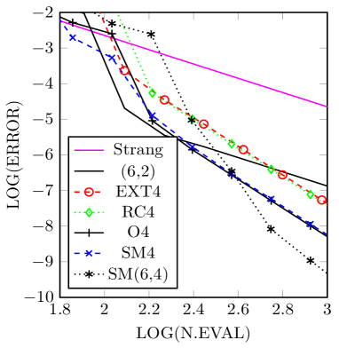
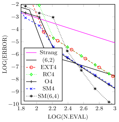
Figure 1: Error versus number of evaluations of $\Phi^{[h]}_{A}$ for the numerical integration in Example 1 at $t=2\pi$ for $\varepsilon=\frac{1}{4}$ (left panel) and $\varepsilon=\frac{1}{10}$ (right panel).

Example 2: A linear parabolic equation.

The next test-problem is the following scalar parabolic equation in one-dimension

$$\frac{\partial u(x,t)}{\partial t}=\alpha(t)^{2}\Delta u(x,t)+V(x,t)u(x,t),\qquad u(x,0)=u_{0}(x),$$ (3.12)

with $u_{0}(x)=\sin(2\pi x)$ and periodic boundary conditions in the space domain $[0,1]$. We take $\alpha(t)=\frac{1}{4}+\mu\cos(wt)$, $V(x,t)=\frac{1}{10}\left(3(1-e^{-t})+\sin(2\pi x)\right)$ and discretize in space

$$x_{j}=j(\delta x),\qquad j=1,\ldots,N\quad\mbox{ with }\quad\delta x=1/N,$$

thus arriving at the differential equation

$$\frac{dU}{dt}=\alpha(t)^{2}AU+B(t)U,$$ (3.13)

where $U=(U_{1},\ldots,U_{N})=(u_{1},\ldots,u_{N})\in\mathbb{R}^{N}$. The Laplacian $\Delta$ has been approximated by the matrix $A$ of size $N\times N$ given by

$$A=\frac{1}{(\delta x)^{2}}\begin{pmatrix}-2&1&&&1\\ 1&-2&1\\ &1&-2&1\\ &&\ddots&\ddots&\ddots\\ 1&&&1&-2\end{pmatrix},$$ (3.14)

and $B(t)=\mbox{diag}(V(x_{1},t),\ldots,V(x_{N},t))$. We take $\mu=1/6,\ w=2$, $N=100$ points and compare different composition methods by computing the corresponding approximate solution on the time interval $[0,1]$. We compute the $2$-norm error of the numerical solution with respect to the exact solution of the semidiscretised equation (computed numerically up to a sufficiently high accuracy) at time $t=1$. The results are collected in Fig. 2 where the superiority of the splitting methods with complex coefficients is also manifest.

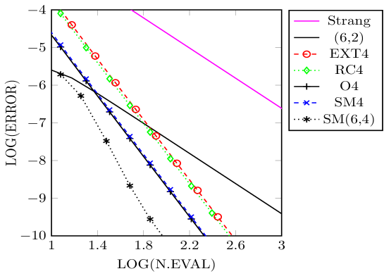
Figure 2: Efficiency comparison between algorithms for the linear parabolic equation (3.12) with parameters $\mu=1/6,w=2$ at final time $t=1$.

Example 3: The semi-linear reaction-diffusion equation of Fisher.

Our final test-problem is the following non-linear parabolic scalar equation in one-dimension

$$\frac{\partial u}{\partial t}=\alpha(t)^{2}\Delta u+F(u,t),\qquad u(x,0)=u_{0}(x),$$ (3.15)

with periodic boundary conditions in the space domain $[0,1]$. We take, in particular, the Fisher’s potential

$$F(u)=\gamma(t)u(1-u),$$

with $\gamma(t)=(2-e^{-\beta t})/100$ and $\alpha(t)=\frac{1}{4}+\mu\cos(wt)$.

The splitting considered here corresponds to solving, on one hand, the linear equation with $A$ given by (3.14) and on the other hand, the nonlinear ordinary differential equation

$$\frac{\partial u}{\partial t}=\gamma(t)u(1-u)$$

with initial condition $u(x,0)=u_{0}(x).$ After discretization in space, we arrive at the differential equation

$$\frac{dU}{dt}=\alpha(t)^{2}AU+F(U,t),$$ (3.16)

where $U=(U_{1},\ldots,U_{N})=(u_{1},\ldots,u_{N})\in\mathbb{R}^{N}$, A is a circulant matrix of size $N\times N$ as in the the previous linear case and $F(U,t)$ is now defined by

$$F(U,t)=\gamma(t)\big{(}U_{1}(1-U_{1}),\ldots,U_{N}(1-U_{N})\big{)}.$$

Here we consider splitting technique (2.11) as

$$\left\{\begin{array}[]{l}U^{\prime}=\alpha(t_{1})^{2}AU\\ t_{1}^{\prime}=1\end{array}\right.\qquad\mbox{ and }\qquad\left\{\begin{array}[]{l}U^{\prime}=\gamma_{1}U(1-U)\\ t_{1}^{\prime}=0.\end{array}\right.$$ (3.17)

where $\gamma_{1}=\gamma(t_{1})$. Since $\gamma(t)$ is frozen at real values of $t$, it must be considered as a constant, and the scalar equations can be solved analytically

$$u(x,h)=u_{0}(x)\frac{\e^{\gamma_{1}h}}{1+u_{0}(x)(\e^{\gamma_{1}h}-1)}\ ,$$

which is well defined for small complex time $h$. We proceed in the same way as for the previous linear case, starting with $u_{0}(x)=\sin(2\pi x)$.

We choose $\beta=1,\mu=1/6,\ w=2$, $N=100$ and compute the error at the final time $t=1$ by applying the same composition methods as in the linear case. The results are collected in Fig. 3.

Figure 3: Efficiency comparison between algorithms for the equation of Fisher with parameters $\beta=1,\mu=1/6,w=2$ at final time $t=1$.

4 Conclusions

We have considered the numerical integration of non-autonomous separable parabolic equations using high order splitting methods with complex coefficients. A straightforward application of splitting methods with complex coefficients to non-autonomous problems require the evaluation of the time-dependent functions on the operators at complex times, and the corresponding flows in the numerical scheme are, in general, not well conditioned. To avoid this trouble, in this work we consider a class of methods in which one set of the coefficients belong to the class of real and positive numbers. Taking the time as a new coordinate and an appropriate splitting of the system allows us to build numerical schemes where all time-dependent operators are evaluated at real values of the time. This technique shows a great interest for perturbed systems, and this problem is analysed in more detail. In this case, the flow of the dominant part has to be advanced using the real coefficients. We have analysed the algebraic structure of the problem and the cost of the algorithms in order to build efficient high order methods, and some few new methods are reported as an illustration. Higher order and more efficient methods require a considerably deeper analysis, and methods belonging to this class as well as more general methods are being considered by the authors of Ref. [5] and will be published elsewhere. Several numerical examples are considered where it is shown the good performance of this class of methods. We have shown that splitting methods with complex coefficients can also be used on non-autonomous non-linear parabolic problems and they can show a good performance so, high order and more efficient schemes following the guidelines presented in this work can be of great interest. We must also remark that order reductions are expected for problems with Dirichlet or Newman boundary conditions on bounded domains, and the performance of high order methods on these problems diminishes, being an interesting problem that needs further investigation.

References

- [1] P. Bader and S. Blanes, Fourier methods for the perturbed harmonic oscillator in linear and nonlinear Schrödinger equations. Phys. Rev. E. 83, 046711 (2011).
- [2] A.D. Bandrauk, E. Dehghanian, and H. Lu, Complex integration steps in decomposition of quantum exponential evolution operators. Chem. Phys. Lett., 419 (2006), pp. 346–350.
- [3] A.D. Bandrauk and Hai Shen, Improved exponential split operator method for solving the time-dependent Schrödinger equation. Chem. Phys. Lett., 176 (1991), pp. 428–432.
- [4] S. Blanes and F. Casas, On the necessity of negative coefficients for operator splitting schemes of order higher than two. Appl. Num. Math., 54 (2005), pp. 23–37.
- [5] S. Blanes, F. Casas, P. Chartier and A. Murua, Optimized high-order splitting methods for some classes of parabolic equations. Math. Comput., 82 (2013), pp. 1559–1576.
- [6] S. Blanes, F. Casas, A. Farrés, J. Laskar, J. Makazaga and A. Murua, New families of symplectic splitting methods for numerical integration in dynamical astronomy. Appl. Numer. Math., 68, (2013), pp. 58–72.
- [7] S. Blanes, F. Casas, and M. Thalhammer, Work in Progress.
- [8] S. Blanes, F. Diele C. Maragni, and S. Ragni, Splitting and composition methods for explicit time dependence in separable dynamical systems. J. Comput. Appl. Math., 235, (2010), pp. 646–659.
- [9] S. Blanes and P.C. Moan, Splitting Methods for non-autonomous differential equations, J. Comput. Phys., 170, (2001), pp. 205–230.
- [10] S. Blanes,P. C. Moan, Fourth-and sixth-order commutator-free Magnus integrators for linear and non-linear dynamical systems. Appl. Numer. Math., 56, (2006), pp. 1519–1537.
- [11] J. Candy and W. Rozmus, A symplectic integration algorithm for separable Hamiltonian functions, J. Comp. Phys., 92 (1991), pp. 230-256.
- [12] F. Castella, P. Chartier, S. Descombes, and G. Vilmart, Splitting methods with complex times for parabolic equations. BIT, 49 (2009), pp. 487–508.
- [13] J. E. Chambers, Symplectic integrators with complex time steps. Astron. J., 126 (2003), pp. 1119–1126.
- [14] M. Creutz and A. Gocksch, Higher-order hybrid Monte Carlo algorithms. Phys. Rev. Lett., 63 (1989), pp. 9–12.
- [15] D. Goldman and T. J. Kaper, th-order operator splitting schemes and nonreversible systems. SIAM J. Numer. Anal., 33 (1996), pp. 349–367.
- [16] E. Hansen and A. Ostermann, Exponential splitting for unbounded operators. Math. Comp., 78 (2009), pp. 1485–1496.
- [17] E. Hansen and A. Ostermann, High order splitting methods for analytic semigroups exist. BIT, 49 (2009), pp. 527–542.
- [18] R.I. McLachlan, Composition methods in the presence of small parameters, BIT, 35 (1995), pp. 258–268.
- [19] R.I. McLachlan and R. Quispel, Splitting methods. Acta Numerica, 11 (2002), pp. 341–434.
- [20] T. Prosen and I. Pizorn, High order non-unitary split-step decomposition of unitary operators. J. Phys. A: Math. Gen., 39 (2006), pp. 5957–5964.
- [21] Q. Sheng, Solving linear partial differential equations by exponential splitting. IMA J. Numer. Anal., 9 (1989), pp. 199–212.
- [22] M. Suzuki, Fractal decomposition of exponential operators with applications to many-body theories and Monte Carlo simulations. Phys. Lett. A, 146 (1990), pp. 319–323.
- [23] M. Suzuki, General theory of fractal path integrals with applications to many-body theories and statistical physics. J. Math. Phys., 32 (1991), pp. 400–407.
- [24] M. Suzuki, Hybrid exponential product formulas for unbounded operators with possible applications to Monte Carlo simulations. Phys. Lett. A, 201 (1995), pp. 425–428.
- [25] M. Thalhammer, A fourth-order commutator-free exponential integrator for nonautonomous differential equations. SIAM J.Numer. Anal., 44 (2006), pp. 851–864.
- [26] H. Yoshida, Construction of higher order symplectic integrators. Phys. Lett. A, 150 (1990), pp. 262–268.