Systematic properties of decelerating relativistic jets in low-luminosity radio galaxies

Abstract

We model the kiloparsec-scale synchrotron emission from jets in 10 Fanaroff-Riley Class I radio galaxies for which we have sensitive, high-resolution imaging and polarimetry from the Very Large Array. We assume that the jets are intrinsically symmetrical, axisymmetric, decelerating, relativistic outflows and we infer their inclination angles and the spatial variations of their flow velocities, magnetic field structures and emissivities using a common set of fitting functions. The inferred inclinations agree well with independent indicators. The spreading rates increase rapidly, then decrease, in a flaring region. The jets then recollimate to form conical outer regions at distance $r_{0}$ from the active galactic nucleus (AGN). The flaring regions are homologous when scaled by $r_{0}$. At $\approx$0.1$r_{0}$, the jets brighten abruptly at the onset of a high-emissivity region and we find an outflow speed of $\approx$0.8$c$, with a uniform transverse profile. Jet deceleration first becomes detectable at $\approx$0.2$r_{0}$ and the outflow often becomes slower at its edges than it is on-axis. Deceleration continues until $\approx$0.6$r_{0}$, after which the outflow speed is usually constant. The dominant magnetic-field component is longitudinal close to the AGN and toroidal after recollimation, but the field evolution is initially much slower than predicted by flux-freezing. In the flaring region, acceleration of ultrarelativistic particles is required to counterbalance the effects of adiabatic losses and account for observed X-ray synchrotron emission, but the brightness evolution of the outer jets is consistent with adiabatic losses alone. We interpret our results as effects of the interaction between the jets and their surroundings. The initial increase in brightness occurs in a rapidly falling external pressure gradient in a hot, dense, kpc-scale corona around the AGN. We interpret the high-emissivity region as the base of a transonic ‘spine’ and suggest that a subsonic shear layer starts to penetrate the flow there. Most of the resulting entrainment must occur before the jets start to recollimate.

1 Introduction

Jets from active galactic nuclei (AGNs) are important in many areas of astrophysics: they extract energy from supermassive black holes, produce the most energetic photons (and perhaps cosmic rays) we observe, act as conveyors of ultrarelativistic particles and magnetic fields from the parsec-scale environments of AGN to the multi-kiloparsec scales of extended radio galaxies and quasars, and supply copious amounts of energy to their surroundings, thereby preventing cooling and profoundly affecting the evolution of massive galaxies and clusters.

AGN jets are relativistic where they are first formed (Boettcher et al., 2012, and references therein). In this paper, we are concerned with jets in low-luminosity radio galaxies, whose flows are initially relativistic (e.g. Biretta et al. 1995; Giovannini et al. 2001; Hardcastle et al. 2003), but rapidly decelerate on kiloparsec scales (e.g. Laing et al. 1999).

We have made deep Very Large Array (VLA) observations of twin radio jets in nearby, low-luminosity radio galaxies with Fanaroff & Riley (1974) Class I (FR I) morphology, in which we can image both jets with high angular resolution transverse to their axes. Our goal is to understand the kinematics and dynamics of these jets. There are, as yet, no predictive theoretical models for FR I jets on kiloparsec scales. The problem of simulating the propagation of a very light, relativistic, magnetized jet in three dimensions is computationally prohibitive, with poorly known initial conditions: no simulation can yet hope to follow a jet all the way from its formation on scales comparable with the gravitational radius of the central black hole to the kiloparsec scales for which the most detailed observations are available. We have therefore adopted an empirical approach to jet modelling in which we attempt to infer basic flow parameters without introducing too many preconceptions about the underlying physics.

The jets we have observed exhibit systematic side-to-side asymmetries in total intensity and linear polarization that can be recognized as large-scale manifestations of Special Relativistic aberration. Our key assumption is that apparent asymmetries due to aberration are much larger than any intrinsic asymmetries over the faster parts of the jets. Specifically, we assume that the jets can be approximated as intrinsically symmetrical, axisymmetric, relativistic, stationary flows in which the magnetic fields are disordered but anisotropic. We adopt simple, parametrized functional forms for the geometries, velocity fields, intrinsic emissivity variations and three-dimensional magnetic field configurations of the outflows, calculate model brightness distributions and optimize the parameters by fitting to our observed $I$, $Q$ and $U$ images. Our kinematic models are described in a series of papers (Laing & Bridle, 2002a; Canvin & Laing, 2004; Canvin et al., 2005; Laing et al., 2006b; Laing & Bridle, 2012), where we present evidence for deceleration from relativistic to sub-relativistic speeds on kiloparsec scales. Starting from these kinematic models, we have also addressed the dynamics of jet deceleration using a conservation-law approach (Laing & Bridle, 2002b; Wang et al., 2009).

We now wish to look for systematic similarities and differences between the flow properties deduced by these methods for FR I radio galaxies with different luminosities and in different environments. During the course of our project, it became clear that some of the functional forms we had used in earlier papers were insufficiently general while others were unnecessarily complicated. Changes to the fitting functions that we had made as we refined our approach made it difficult to compare our results systematically across all of the sources we had observed. In this paper, we use the same set of fitting functions for all of the sources.

In Section 2, we give the essential information about the sources and our observational material. We outline the model-fitting technique in Section 3 and show comparisons between data and models in Section 4 in a way that emphasizes the systematic variation of the appearance of these jets with their inferred orientation to the line of sight. The results of the model fits are presented and described in Section 5. Consistency tests are outlined in Section 6 and the effects of intrinsic asymmetries on our results are explored in Section 7. We discuss the implications for jet physics in Section 8 and summarize our conclusions in Section 9. The fitting functions are listed for reference in Appendix A. The $\chi^{2}$ values for the fits are tabulated and plotted in Appendix B and Appendix C gives notes on individual model fits, emphasizing any differences from our published work. Vector images illustrating the polarization fits are shown in Appendix D. The model parameters and their errors are tabulated in Appendix E.

2 Observations and Image Processing

2.1 Source selection

We seek to model the jets in the subset of FR I radio galaxies whose large scale structure is currently fed by jets that: (a) have propagated far from their AGN, (b) are detectable and resolvable by polarimetry with the VLA on both sides of the nucleus and (c) are reasonably straight. These are the twin-jet sources as classified by Laing (1993) and Leahy (1993). Our selection eliminates some classes of radio source entirely (e.g. relic emission without jets, relaxed doubles whose jets disrupt very close to the nucleus, wide-angle tails and other objects whose jets remain well collimated and asymmetric until they disrupt, narrow-angle tails and any sources that are confined to the nuclear regions of their galaxies). For the 3CRR and B2 samples, roughly 35% and 46%, respectively, of the FR I sources are of the twin-jet type (Laing, Riley & Longair, 1983; Parma et al., 1987; Leahy, Bridle & Strom, 2000).

Table 1: Basic data for the sources in this paper. (1) Name as used in this paper; (2) alternative names; (3) redshift (bracketed if the distance is derived from a redshift-independent indicator); (4) metric distance; (5) linear scale, in kpc arcsec^-1; (6) references for redshift and distance.

Name	Alt.	$z$	$D$	Scale	Ref
	name		Mpc	kpc
				arcsec-1
1553+24		0.04263	180.8	0.841	7
0755+37	NGC 2484	0.04284	181.7	0.845	3
0206+35	UGC 1651	0.03773	160.2	0.748	2
	4C35.03
NGC 315		0.01649	70.4	0.335	5
3C 31	NGC 383	0.01701	72.6	0.346	6
NGC 193	UGC 408	0.01472	62.8	0.300	4
M 84	3C 272.1	(0.0035)	18.5	0.089	1,6
	NGC 4374
0326+39		0.02430	103.5	0.490	3
3C 296	NGC 5532	0.02470	105.2	0.498	3
3C 270	NGC 4261	(0.007465)	30.8	0.148	1,6
3C 449		0.017085	72.9	0.347	7

References: (1) Cappellari et al. (2011); (2) Falco et al. (1999); (3) Miller et al. (2002); (4) Ogando et al. (2008); (5) Smith et al. (2000); (6) Trager et al. (2000); (7) de Vaucouleurs et al. (1991)

We selected 10 twin-jet sources by the following criteria.

1. The jets are either straight and antiparallel or bend by sufficiently small angles that the images can be ‘straightened’ by a simple transformation (Section 2.3.1; Laing & Bridle, in preparation).

2. Any surrounding lobe emission is sufficiently weak to be subtracted using a simple linear interpolation across the jets (Section 2.3.2; Laing & Bridle, 2012).

3. There are significant brightness and polarization asymmetries in the jet bases for our models to fit.

4. The polarized emission from both jets can be imaged with adequate signal-to-noise ratio. This is essential in order to break the degeneracy between velocity and angle to the line of sight (Section 3.2).

We also show observations for one source we cannot model, 3C 449. This has highly symmetrical jets and is likely to be a side-on counterpart of the other sources, so we include it in studies of trends with inclination.

The sources considered here are listed in Table 1 in order of increasing fitted angle to the line of sight (Section 5), together with their redshifts and linear scales. For the two nearest galaxies, we adopted redshift-independent distances (Cappellari et al., 2011, and references therein). In the remaining cases, we derived the distances directly from the quoted redshifts without further correction, assuming a concordance cosmology with $H_{0}$ = 70 $\rm{km\,s^{-1}\,Mpc^{-1}}$, $\Omega_{\Lambda}=0.7$ and $\Omega_{\rm M}=0.3$.

2.2 Images

High-quality VLA images at 4.9 or 8.5 GHz are available for all of the sources. We started from images of Stokes $I$, $Q$ and $U$ at one or two resolutions. We then corrected the observed ${\mn@boldsymbol{E}}$-vector position angles for Faraday rotation using multifrequency, high-resolution rotation-measure (RM) images (except for 0326+39 and 1553+24, for which the corrections are close to zero) and checked that residual depolarization is negligible. From the corrected position angles, $\chi_{0}$, we derived zero-wavelength $Q$ and $U$ images: $Q_{0}=P\cos 2\chi_{0}$ and $U_{0}=P\sin 2\chi_{0}$, where $P=(Q^{2}+U^{2})^{1/2}$ is the polarized intensity. We fit to $I$, $Q_{0}$ and $U_{0}$ (from now on we drop the suffices). We define the direction of the apparent magnetic field to be $\chi_{0}+\pi/2$ (this is the same as the projected position angle on the sky for a uniform magnetic field, but not in the general case of an integration along the line of sight) and the scalar degree of polarization to be $p=P/I$.

In Table 2, we list the model fields and the sizes, resolutions and intensity ranges of the images displayed in this paper. We also give references to descriptions of the observations, data reduction, Faraday rotation correction and modelling.

Table 2: Radio data, image parameters and associated references. (1) Name; (2) label used in the figures; (3) $\log$ of the luminosity in extended emission at an emitted frequency of 1.4 GHz, in W Hz^-1; (4) observing frequency for the modelled images, in GHz; (5) model field, in arcsec; (6) – (8) refer to the lower-resolution images used for modelling and specifically to the plots in Figs 3 – 5 and 27; (6) beamwidth (FWHM, arcsec); (7) field size along the jet axis as plotted in the figures; (8) total-intensity maximum for Fig. 3; (9) – (11): as (6) – (8), but for the higher-resolution images; (12) references to radio observations and models.

Name		$\log(P_{\rm ext}$	$\nu$	Model	Resolution 1			Resolution 2			Refer-
		W Hz${}^{-1})$	GHz	field	FWHM	Field	$I_{\rm max}$	FWHM	Field	$I_{\rm max}$	ences
				arcsec	arcsec	arcsec	mJy	arcsec	arcsec	mJy
							beam-1			beam-1
1553+24	a	23.79	8.5	60.0	0.75	57.5	1.0	0.25	9.6	2.00	1
0755+37	b	25.02	4.9	66.0	1.30	63.0	3.0	0.40	10.0	5.0	8,10
0206+35	c	24.82	4.9	22.0	0.35	21.0	3.0				8,10
NGC 315	d	24.58	4.9	200.0	2.35	190.0	10.0	0.40	38.0	1.25	2, 7,11
3C 31	e	24.54	8.4	56.0	0.75	54.0	3.0	0.25	20.0	1.00	5, 8
NGC 193	f	23.96	4.9	120.0	1.35	117.0	3.0	0.45	17.0	1.50	9,11
M 84	g	23.42	4.9	40.0	0.40	25.0	3.0				9,11
0326+39	h	24.27	8.5	43.5	0.50	42.0	0.5	0.25	15.0	0.2	1, 9
3C 296	i	24.76	8.5	83.4	0.75	81.9	1.5	0.25	15.0	0.5	6, 9
3C 270	j	24.32	4.9	82.0	0.60	80.0	0.75				12
3C 449	k	24.38	8.5		1.25	90.0	1.5	0.80	52.5	1.0	3, 4

References for Table 2: 1 Canvin & Laing (2004); 2 Canvin et al. (2005); 3 Feretti et al. (1999); 4 Guidetti et al. (2010); 5 Laing & Bridle (2002a); 6 Laing et al. (2006b); 7 Laing et al. (2006a); 8 Laing et al. (2008a); 9 Laing et al. (2011); 10 Laing & Bridle (2012); 11 Laing & Bridle (in preparation); 12 Laing, Guidetti & Bridle (in preparation);

2.3 Complications: the symmetry assumption and bent jets, lobe subtraction, small-scale structure and backflow

2.3.1 The symmetry assumption and bent jets

Even if jets are exactly symmetrical where they are first formed, interactions between them and their environment introduce asymmetries and often become the dominant shapers of the large-scale radio structure. We aim to identify and model only those parts of the jets near the nucleus where relativistic effects dominate the observed asymmetries and to quantify the errors introduced by residual environmental effects.

For that reason, we initially restricted our modelling to straight, antiparallel jets. In some FR I sources, the jets bend in projection on the sky by small angles while maintaining their collimation, and these bends occur at discrete locations rather than forming continuously-curved ridge-lines. In such cases it is possible to ‘straighten’ the jets by a simple image transformation (Laing & Bridle, in preparation) in which the brightness distribution maintains its initial position angle up to some distance from the AGN, after which it is sheared in a constant direction in such a way that the ridge-line is rotated by a constant angle $\Delta$. This type of distortion is a position-dependent translation and therefore preserves surface brightness. We implement the transformation by polynomial interpolation of the brightness distributions in all three Stokes parameters, together with a rotation of the ${\mn@boldsymbol{E}}$-vector position angle by $-\Delta$ which in turn modifies $Q$ and $U$. After this transformation, $I$, $Q$ and $U$ all have the expected symmetries with respect to the projection of the jet axis on the sky.

This approach has allowed us to extend our earlier modelling of NGC 315 (Canvin et al., 2005) to larger distances, to improve our model for 3C 296 (Laing et al., 2006b) and to derive new models for NGC 193 and M 84. The images for these four sources shown below have all been corrected in this way. Additional uncertainties are obviously introduced by the use of a bending correction: we cannot determine the extent to which jets bend perpendicular to the plane of the sky (and hence any change in Doppler factor) and there may be other deviations from intrinsic symmetry. In NGC 315, 3C 296 and NGC 193, we expect these uncertainties to be small: the bends are $\leq$5^∘ in projection and/or restricted to the outermost parts of the jets which have low weight in the modelling. For M 84, the bends are both larger in amplitude ($5^{\circ}$ and $14^{\circ}$ for the main and counter-jets, respectively) and much closer to the nucleus, so larger errors are likely. Full details will be given by Laing & Bridle (in preparation).

2.3.2 Lobe subtraction

The jets in the majority of sources discussed here are surrounded, at least in projection, by extended lobes. In order to model the jets, any superposed lobe emission must be removed in all Stokes parameters. One possible approach is to exploit the spectral differences between jet and lobe emission; a second is to assume that the lobe emission varies slowly across the jet, and to use spatial interpolation to perform the subtraction (see Laing & Bridle 2012 for a comparison of these methods). We found that the latter approach gave superior results in all cases. We have applied it to all of the images in which there is significant lobe emission at the lower (or only) resolution used for modelling. The sources affected are: 0206+35, 0755+37, NGC 193, M 84, 3C 296 and 3C 270. We show only images after lobe subtraction. Full details are given by Laing & Bridle (2012, and in preparation) and Laing et al. (in preparation).

2.3.3 Small-scale structure

Conceptually, we assume stationary flow. In reality, all jets develop small-scale, stochastic structure. Our aim is not to describe the fluctuations, but rather to average over a complex and presumably time-variable flow pattern in such a way as to recover global structure in the brightness and polarization distributions. Our estimates of the flow parameters will be inaccurate if the brightness distributions are dominated by small numbers of compact features, especially if, as we would expect, they are not symmetrically located with respect to the AGN. We seek to mitigate this problem by identifying and fitting common features in the brightness and polarization distributions of multiple sources. We do not expect stochastic variations to bias the mean flow parameters for a sample of sources, since they should be uncorrelated with inclination.

2.3.4 Backflow

Many FR I radio galaxies have outer structures resembling the lobes of FR II sources, but without the compact hot-spots that are thought to mark the terminations of high-Mach-number jets. Our observations of two sources of this type, 0206+35 and 0755+37 (Laing et al., 2011; Laing & Bridle, 2012), revealed that the jets in both sources have two-component structures transverse to their axes. Close to the axis, the main jets are centre-brightened whereas the counter-jets are centre-darkened. Both are surrounded by broader collimated emission that is brighter on the counter-jet side. We modelled these jets as decelerating, relativistic outflows surrounded by slower (but still mildly relativistic) backflows (Laing & Bridle, 2012). In this paper, we are concerned primarily with the outflows and their relation to similar structures in other sources. When comparing models with observations, we perforce include the backflow component (otherwise we could not find an acceptable fit), but with the primary purpose of isolating and fitting the outflow. We do not duplicate our earlier, detailed discussion of backflow properties (Laing & Bridle, 2012).

3 Model fits

3.1 Assumptions

We make the following assumptions when calculating model brightness distributions.

1. The jets are intrinsically symmetrical, axisymmetric, stationary flows. After cosmological corrections are applied, the jet boundary is at rest in the observer’s frame.

2. The flow is laminar. If (as seems likely) the real flow has significant random motions, then we will determine average parameters weighted by the observed-frame emissivity.

3. The emission is optically thin synchrotron radiation. We do not include optically thick emission from the core in the model.

4. The radiating particles have a power-law energy distribution

   $$n(E){\rm d}E = n_{0}E^{-q}{\rm d}E$$ (1)

   with $q=2\alpha+1$, corresponding to a constant spectral index $\alpha$ with $I(\nu)\propto\nu^{-\alpha}$. In practice, we use the mean spectral index for the jets in a given source over the modelled region in our frequency range. This is a good approximation for all of our sources, for which $\alpha\approx 0.6$ (Laing & Bridle, 2013).

5. The pitch-angle distribution of the radiating electrons is random, in which case the maximum observed degree of polarization is $p_{0}=(3\alpha+3)/(3\alpha+5)\approx 0.7$.

6. The magnetic field is disordered on small scales, with many reversals, but anisotropic. We quantify the anisotropy using the two independent ratios of the rms field components along three orthogonal directions defined with respect to the flow streamlines. Both vector-ordered and disordered fields can produce high degrees of polarization. As we will show, the dominant field components are toroidal and longitudinal. Large-scale helical fields (with significant longitudinal as well as toroidal components) are inconsistent with observations because the distributions of angles between the field and the line of sight are different on opposite sides of the jet ridge-line and the transverse profiles of total intensity and linear polarization consequently show systematic asymmetries (Laing, 1981; Laing, Canvin & Bridle, 2003). They are also unlikely on such large scales because the longitudinal magnetic flux close to the AGN would then be unreasonably large (Begelman, Blandford & Rees, 1984). The combination of ordered toroidal and disordered longitudinal components would produce the same emission as a purely disordered configuration, however. We cannot distinguish between these two cases (and others with symmetrical field-angle distributions), but our estimates of field component ratio are essentially independent of the details of the configuration.

7. We define the scalar emissivity function

   $$\epsilon = n_{0}B^{1+\alpha},$$ (2)

   where $B$ is the rms total magnetic field (all quantities are defined in the rest frame). It is multiplied by a constant and by functions depending on the field structure to give the true emissivities $e$ in $I$, $Q$ or $U$ (Section 3.2).

8. Variations of velocity and field-ordering with position are smooth. We allow limited discontinuities in the emissivity function.

3.2 Principles

The key to our method is to determine the velocity and inclination angle independently by comparing emission from the main and counter-jets in both total intensity and linear polarization. For an emitting element moving at an angle $\theta$ to the line of sight ($0\leq\theta\leq\pi$, with $\theta=0$ towards the observer) and observed at frequency $\nu$, the emissivity $e$ in the observer’s frame is given by

$$e(\theta,\nu) = D^{2}(\theta)e^{\prime}(\theta^{\prime},\nu^{\prime}),$$ (3)

where $e^{\prime}$, $\theta^{\prime}$ and $\nu^{\prime}$ are measured in the rest frame of the emitting material (Begelman et al., 1984, equation C6). $D$ is the Doppler factor, which also relates the frequencies in the observed and rest frames:

$$D(\theta) = [\Gamma(1-\beta\cos\theta)]^{-1}$$ (4)

$$\nu = D(\theta)\nu^{\prime}.$$ (5)

Here, $\beta c$ is the bulk flow speed and $\Gamma=(1-\beta^{2})^{-1/2}$ is the bulk Lorentz factor. The angles to the line of sight in the two frames are related by

$$\sin\theta^{\prime} = D(\theta)\sin\theta.$$ (6)

For an optically thin source at distance $d$ with a power-law spectrum of spectral index $\alpha$ as defined in Section 3.1, the observed flux density $S$ is

$$S(\theta,\nu) = D^{2+\alpha}\int e^{\prime}(\theta,\nu){\rm d}V/d^{2}$$ (7)

The integration is performed in the observer’s frame, for which $dV$ is the volume element (Begelman et al., 1984, equation C7).

From now on, we consider antiparallel jets and take $\theta$ ($0\leq\theta\leq\pi/2$) to be the angle to the line of sight for the approaching one. The Doppler factors for the approaching and receding jets, $D_{\rm j}$ and $D_{\rm cj}$ are

$$D_{\rm j} = [\Gamma(1-\beta\cos\theta)]^{-1}$$ (8)

$$D_{\rm cj} = [\Gamma(1+\beta\cos\theta)]^{-1}$$ (9)

For isotropic emission in the rest frame, the jet/counter-jet ratio is then given by the well-known formula

$$\frac{I_{\rm j}}{I_{\rm cj}} = \left(\frac{1+\beta\cos\theta}{1-\beta\cos\theta}\right)^{2+\alpha}$$ (10)

We cannot determine $\beta$ and $\theta$ independently from this ratio alone. In general, however, emission is anisotropic in the rest frame and the angular dependences are different for the three Stokes parameters. This allows us to separate the two quantities.

In order to illustrate this point, we analyse two simple field configurations for which there are analytical expressions for the total and polarized intensity and which are good initial approximations to those we find in FR I jets (Section  5.4). We consider the idealized case of cylindrical, antiparallel jets with constant velocity. The field configurations are assumed not to vary along the jets and the particle densities and rms field strengths are independent of position. We also take $\alpha=1$ in order to simplify the formulae. We choose the zero-point of ${\mn@boldsymbol{E}}$-vector position angle to be the projection of the jet axis on the plane of the sky, so that $U=0$. The two configurations are as follows:

1. a field which has no longitudinal component, but which is orientated randomly in planes perpendicular to the jet axis (Laing, 1981, Section IIIa) and

2. a field which is orientated randomly within shells of given radius, but with no component perpendicular to the jet axis (Laing, 1981, Section IIIb, model B).

In the first configuration, the apparent magnetic field is always perpendicular to the jet axis ($Q>0$):

$$Q(\theta^{\prime}) = Kp_{0}\sin^{2}\theta^{\prime}$$ (11)

$$I(\theta^{\prime}) = K(2-\sin^{2}\theta^{\prime})$$ (12)

($K$ varies across the jet, but is the same for both Stokes parameters). In the observed frame, the ratios of polarized and total intensity are

$$\frac{Q_{\rm j}}{Q_{\rm cj}} = \left(\frac{D_{\rm j}}{D_{\rm cj}}\right)^{5}$$ (13)

$$= \left(\frac{1+\beta\cos\theta}{1-\beta\cos\theta}\right)^{5}$$

$$\frac{I_{\rm j}}{I_{\rm cj}} = \left(\frac{D_{\rm j}}{D_{\rm cj}}\right)^{3}\frac{2-D_{\rm j}^{2}}{2-D_{\rm cj}^{2}}$$ (14)

$$= \left(\frac{1+\beta\cos\theta}{1-\beta\cos\theta}\right)^{3}\frac{2-(1-\beta^{2})(1+\beta\cos\theta)^{-2}}{2-(1-\beta^{2})(1-\beta\cos\theta)^{-2}}$$

The degree of polarization in the approaching jet always exceeds that in the receding jet.

In the second configuration, the degree of polarization varies perpendicular to the jet. On-axis, the apparent magnetic field is again always transverse, and we have the same relations as in equations (11) and (12), but with $\theta^{\prime}$ offset by $\pi/2$:

$$Q(\theta^{\prime}) = Kp_{0}(1-\sin^{2}\theta^{\prime})$$ (15)

$$I(\theta^{\prime}) = K(1+\sin^{2}\theta^{\prime})$$ (16)

Consequently, the emission ratios in the observed frame are

$$\frac{Q_{\rm j}}{Q_{\rm cj}} = \left(\frac{D_{\rm j}}{D_{\rm cj}}\right)^{3}\frac{1-D_{\rm j}^{2}\sin^{2}\theta}{1-D_{\rm cj}^{2}\sin^{2}\theta}$$ (17)

$$= \left(\frac{1+\beta\cos\theta}{1-\beta\cos\theta}\right)^{3}\frac{1-(1-\beta^{2})(1-\beta\cos\theta)^{-2}}{1-(1-\beta^{2})(1+\beta\cos\theta)^{-2}}$$

$$\frac{I_{\rm j}}{I_{\rm cj}} = \left(\frac{D_{\rm j}}{D_{\rm cj}}\right)^{3}\frac{1+D_{\rm j}^{2}\sin^{2}\theta}{1+D_{\rm cj}^{2}\sin^{2}\theta}$$ (18)

$$= \left(\frac{1+\beta\cos\theta}{1-\beta\cos\theta}\right)^{3}\frac{1+(1-\beta^{2})(1-\beta\cos\theta)^{-2}}{1+(1-\beta^{2})(1+\beta\cos\theta)^{-2}}$$

If $\beta=\cos\theta$, the degree of polarization in the approaching jet $p_{\rm j}=|Q_{\rm j}|/I_{\rm j}=0$ (equation 17), whereas the receding jet has $p_{\rm cj}=2p_{0}\cos^{2}\theta/(1+\cos^{4}\theta)$ with a transverse apparent field (equations 15 and 16). At the edges of both jets, $Q/I=-p_{0}$ (longitudinal apparent field) and

$$\frac{I_{\rm j}}{I_{\rm cj}} = \frac{Q_{\rm j}}{Q_{\rm cj}}$$ (19)

$$= \left(\frac{D_{\rm j}}{D_{\rm cj}}\right)^{3}$$

$$= \left(\frac{1+\beta\cos\theta}{1-\beta\cos\theta}\right)^{3}$$

as in the isotropic case.

If we knew the field configuration a priori, we could use pairs of equations such as (13) and (14) or (17) and (18) to determine $\beta$ and $\theta$ independently. In practice, of course, the field configuration is unknown. The additional constraints we use to determine it are the transverse variations of total intensity and linear polarization across the two jets: profiles across both jets are necessary in order to provide integrations through the field distributions at different angles to the line of sight in the rest frame.

3.3 Resolving degeneracies using transverse profiles

It is clearly important to check whether the same observed brightness distributions (in $I$, $Q$ and $U$) could be produced by alternative combinations of velocity, magnetic field and emissivity function. First, we note that differences between the approaching and receding jets are barely affected by the form adopted for the emissivity function, which divides out from the jet/counter-jet ratio in any Stokes parameter in the limit of a uniform flow. There is a potential degeneracy between velocity and field structure, however. We infer the presence of a velocity gradient from the centrally-peaked transverse profile of intensity ratio $I_{\rm j}/I_{\rm cj}$ but there is a way to mimic this profile purely from the anisotropy of the rest-frame emission for one special field configuration, which we now discuss.

Even if the jets have uniform velocities, aberration can cause the angle between a well-ordered field and the line of sight in the rest frame, $\psi^{\prime}$, to be much smaller in the approaching jet. The emissivity ($\propto\sin^{1+\alpha}\psi^{\prime}$) is then much lower. If this happens at the edges of the jets but not on-axis, then the jet/counter-jet sidedness-ratio profile will be centrally peaked. Of the field configurations which are qualitatively consistent with the observed linear polarization, the only one that can produce this effect has a dominant toroidal component, with the field loops seen close to edge-on in the rest frame in the approaching jet ($\psi^{\prime}\approx 0$, so $\theta^{\prime}\approx\pi/2$ and $\beta\approx\cos\theta$). Profiles of sidedness ratio and $Q/I$ for this case are shown in Laing & Bridle (2012, their fig. A1). If we mistakenly assumed isotropic emission in the rest frame and did not look at the polarization, we might indeed conclude (incorrectly) that there is a transverse velocity gradient. However, the polarization of the approaching jet produced by this field configuration is not consistent with the observed one. A pure toroidal field always gives transverse apparent field with $p=p_{0}$ on-axis. If the field loops are viewed edge-on in the rest frame, then this extends over the entire width of the jet. In less perfectly aligned cases, transverse field and high polarization are still seen over much of the width of the jet (Laing & Bridle, 2012, Fig. A1). This is rarely observed.

In practice, solutions of this type do not fit our data: even starting with a purely toroidal field and the appropriate velocity to generate the observed transverse sidedness ratio gradients, our fitting algorithm (Section 3.6) converges to solutions with a transverse velocity gradient and a mixture of longitudinal and toroidal field, as only these can reproduce the observed polarization. We have also verified that the velocity gradient is still required even if the field component ratios are allowed to vary across the jets.

We are therefore confident that there are no significant degeneracies between transverse velocity profile and field structure for the jets we have observed and modelled, because the possibilities can be distinguished by their different polarization profiles.

3.4 Terminology

The term flaring is used in two contexts when describing the properties of kiloparsec-scale radio jets: to describe changes in jet geometry and of jet brightness.

Geometrical flaring of a jet refers to significant increases in its apparent spreading rate (opening angle) with increasing distance from the AGN. These changes (inferred from observing the outer isophotes of the jets) appear to be a continuous process on the scales we can resolve (i.e. the opening angle gradually increases, then decreases). Geometrical flaring can thus be ascribed to an extended region of the propagating jet, and the only observed discontinuity appears to be where the jet opening angle becomes constant.

Brightness flaring of kiloparsec-scale jets refers to significant increases in their apparent brightness with increasing distance from the AGN, often following an initial ‘gap’, or extended region in which the radio emission is weak or undetectable. Unlike geometrical flaring, brightness flaring usually has a well-defined onset (especially considering the effects of projection), so we can often define a single brightness flaring point with some precision.

The two phenomena are evidently connected in that the brightness flaring point generally occurs in a part of the flow where the jet opening angle is increasing with distance, i.e. within the geometrically flaring region. The term ‘flaring’ has been used elsewhere (e.g. Bridle 1982; Roberts 1986; Loken et al. 1995; Laing et al. 1999; Jetha, Hardcastle & Sakelliou 2006; Krause et al. 2012; Laing et al. 2011; Laing & Bridle 2012), to describe both phenomena. We continue this practice, but we will explicitly distinguish geometrical flaring and brightness flaring in what follows, to clarify the relationship(s) between them.

3.5 Fitting functions

The functions used to fit the jet outflows have been chosen empirically to have simple algebraic forms which together allow good fits to the brightness and polarization distributions and straightforward estimation of key physical parameters. The characterization of variations along the jets reflects the observation that there are distinct regions within which the quantities that we model (geometry, velocity, emissivity function and field structure) must vary in different ways. The regions are identifiable by changes in:

geometry

(the shapes of the outer isophotes);

velocity

(the gradient of the sidedness ratio);

emissivity function

(the logarithmic slope of the surface brightness) and

field structure

(the gradient of $Q/I$ on-axis).

In the latter two cases, the changes must be common to both jets. The observations thus lead to the concepts of fiducial locations (the boundaries between regions) and fiducial values defined at these locations, both at the centre and edge of the jet. The functional forms are chosen to interpolate smoothly between the fiducial locations and between the centre and edge. The precise form used for the interpolation functions is not critical (within reason) provided that the values at the fiducial locations are correct. For example, we have used different functions to fit the longitudinal and transverse velocity variations in 3C 31, but the inferred velocity field is very similar in all cases (Laing & Bridle, 2002a, their fig. 17, and this paper).

The fiducial distances and values, together with the functional forms, are defined in Sections 3.5.1 – 3.5.4, below. For completeness, we tabulate the complete coordinate definitions and functional forms in Appendix A (Table 5). Distances, angles and velocities are defined in the observer’s frame and intrinsic parameters for field and emissivity function refer to the rest frame of the emitting plasma.

3.5.1 Geometry and coordinate systems

The jet axis is inclined by an angle $\theta$ to the line of sight; $z$ and $x$ are coordinates along and transverse to the jet axis, respectively. We model on a grid whose size, set by the observed image, is fixed in projection on the sky. The corresponding physical size measured along the jet axis, $r_{\rm grid}$, then depends on $\theta$. Motivated by the discussion in Section 3.4, we divide a jet into geometrically flaring and outer regions, as shown in Fig. 1. The geometry is completely defined by the transition distance between the two regions, $r_{0}$, the radius of the jet at the transition between the regions, $x_{0}$, and the opening angle of expansion in the outer region, $\xi_{0}$.

In order to parametrize the spatial variations of velocity, emissivity function and field ordering, we use a coordinate system $(r,s)$ where the index $s$ is constant for a given streamline, running from 0 on-axis to 1 at the jet boundary, and $r$ increases monotonically with distance along it. The distance of a streamline from the jet axis is:

$$x(z,s) = a_{2}(s)z^{2}+a_{3}(s)z^{3}\makebox{~{}~{}~{}~{}(flaring region)}$$ (20)

$$x(z,s) = (z+A)\tan(\xi_{0}s)\makebox{~{}~{}~{}~{}~{}~{}(outer region)}$$ (21)

where $A=x_{0}/\sin\xi_{0}-r_{0}$. In the outer region, $s=\xi/\xi_{0}$, where $\xi$ is the angle between the flow vector and the jet axis. $a_{2}(s)$ and $a_{3}(s)$ are constant along a given streamline and are defined by the conditions that $x(z,s)$ and its derivative with respect to $z$, $x^{\prime}(z,s)$, are continuous at the transition between the two regions. The vertex of the flow in the outer region is displaced from the nucleus by a distance $A$ and the boundary surface between geometrically flaring and outer regions is a sphere of radius $r_{0}+A$ centred on the vertex. This geometry has the natural feature that the streamlines are orthogonal to the boundary surface where they cross it.

The coordinate along a streamline:

$$r = \frac{zr_{0}}{(r_{0}+A)\cos(\xi_{0}s)-A}\hskip 28.45274ptr\leq r_{0}$$ (22)

$$r = \frac{z+A}{\cos(\xi_{0}s)}-A\hskip 64.01869ptr\geq r_{0}$$ (23)

increases monotonically from 0 at the nucleus. The boundary between the flaring and outer regions is at $r=r_{0}$ regardless of the value of $s$. On the jet axis, $r$ is just the distance from the nucleus, $z$.

The geometry and coordinate system are exactly as used in earlier papers in this series (with the special case $A=0$ for 3C 31; Laing & Bridle 2002a).

Figure 1: The geometry of the model jet outflow, showing the flaring and outer regions and the three quantities $r_{0}$, $x_{0}$ and $\xi_{0}$ which define the shape of its outer surface. Three example streamlines are shown: $s=0$ (on-axis), $s=0.5$ and $s=1$ (the outer boundary).

We chose these functional forms as the simplest which match the observed outer isophotes of the jets on scales which we can resolve: an extrapolation of the flaring region geometry to smaller scales would not be consistent with higher-resolution observations, however.

3.5.2 Velocity

Our model velocity field is simplified significantly from those used in earlier papers, where we adopted rather complicated functional forms purely to enforce continuity in acceleration as well as velocity. In fact, a good fit does not require the velocity to vary smoothly, but merely to be continuous. We assume that the velocity is a separable function of distance coordinate and streamline index, $\beta(r,s)=\beta_{r}(r)\beta_{s}(s)$, with $\beta_{s}(0)=1$. The on-axis velocity $\beta_{r}(r)$ (Fig. 2a) is taken to have a constant value $\beta_{1}$ out to a distance $r_{v1}$ and to decrease linearly to $\beta_{0}$ at $r_{v0}$. Thereafter, either uniform acceleration or deceleration to velocity $\beta_{f}$ at $r=r_{\rm grid}$ is allowed. The transverse velocity variation $\beta_{s}(s)$ (Fig. 2b) has a truncated Gaussian form $\beta_{s}(s)=\exp[s^{2}\ln v(r)]$, specified by the fractional edge velocity, $v(r)\leq 1$ [we found that allowing $v(r)>1$ led to problems with the optimization as $\beta$ approached 1]. The precise form assumed for $\beta_{s}(s)$ does not make much difference either to the quality of the fit or to the derived values of $v$, provided that it is reasonably flat on-axis and decreases smoothly towards the edge: two alternatives were compared by Laing & Bridle (2002a). The values of $v(r)$ at the three fiducial distances $r_{v1}$, $r_{v0}$ and $r_{\rm grid}$ are $v_{1}$, $v_{0}$ and $v_{f}$, respectively. $v(r)=v_{1}$ for $r\leq r_{v1}$; intermediate values are determined by linear interpolation in $r$. The complete form for the velocity function is given in Table 5. It is defined by the fiducial distances $r_{v1}$ and $r_{v0}$, the on-axis velocities $\beta_{1}$, $\beta_{0}$ and $\beta_{f}$ and the fractional edge velocities $v_{1}$, $v_{0}$ and $v_{f}$.

Figure 2: Examples of the functional forms used to fit the jet velocity, emissivity function and field-component ratios. (a) On-axis velocity profile. (b) Transverse velocity profiles at the three fiducial distances, with the same on-axis velocities as in panel (a). (c) On-axis profile of the emissivity function $\epsilon=n_{0}B^{1+\alpha}$ (note the logarithmic scales). (d) Normalized transverse profiles of the emissivity function at three fiducial locations. (e) Profiles of the field ratio $j=\langle B^{2}_{r}\rangle^{1/2}/\langle B^{2}_{t}\rangle^{1/2}$ on-axis and at the edge of the jet. (f) Corresponding transverse profiles for the field ratios at the three fiducial distances. The functional form for the field ratio $k=\langle B^{2}_{l}\rangle^{1/2}/\langle B^{2}_{t}\rangle^{1/2}$ is identical.

3.5.3 Emissivity function

As in the case of the velocity, we take the emissivity function $\epsilon$ to be separable: $\epsilon(r,s)=\epsilon_{r}(r)\epsilon_{s}(s)$. $\epsilon_{r}(r)$ has a piecewise power-law dependence on $r$ (Fig. 2c). Close to the nucleus ($r\leq r_{e1}$), the index is $-E_{\rm in}$. At $r=r_{e1}$, the brightness flaring point, a discontinuity of a factor of $g_{1}$ is allowed. The flaring point marks the beginning of the high-emissivity region, with index $-E_{\rm mid}$, which again may end in a discontinuity (a factor of $g_{0}$). Thereafter, $\epsilon_{r}(r)$ is continuous, with indices $-E_{\rm out}$ from $r=r_{e0}$ up to recollimation ($r=r_{0}$) and $-E_{\rm far}$ from $r_{0}$ until the end of the grid.

The transverse variation of emissivity function again has a truncated Gaussian form, $\epsilon_{s}(s)=\exp[s^{2}\ln e(r)]$ (Fig. 2d), but the value of $e(r)$ is allowed to be $\leq$1 (centre-brightening) or $>$1) (limb-brightening). $e(r)=e_{1}$ for $r\leq r_{e1}$ and takes the values $e_{0}$ and $e_{f}$ at $r_{e0}$ and $r_{\rm grid}$, respectively. Intermediate values for $r>r_{e1}$ are determined by linear interpolation. The complete form of the emissivity function is given in Table 5. The defining parameters are the fiducial distances $r_{e1}$, $r_{e0}$; the on-axis slopes $E_{\rm in}$, $E_{\rm mid}$, $E_{\rm out}$, $E_{\rm far}$; the fractional edge emissivities $e_{1}$, $e_{0}$, $e_{f}$ and the discontinuities $g_{1}$, $g_{0}$.

The model emissivity is set to zero within a fixed projected distance from the nucleus to prevent confusion with the unresolved radio core emission, which we do not attempt to model. This corresponds to a linear distance of $r_{\rm min}$ along the jet axis.

3.5.4 Magnetic-field structure

The three rms magnetic-field components in the rest frame are: $\langle B_{l}^{2}\rangle^{1/2}$ (longitudinal, parallel to a streamline), $\langle B_{r}^{2}\rangle^{1/2}$ (radial, orthogonal to the streamline and outwards from the jet axis) and $\langle B_{t}^{2}\rangle^{1/2}$ (toroidal, orthogonal to the streamline in an azimuthal direction). The rms total field strength is $B=\langle B_{l}^{2}+B_{r}^{2}+B_{t}^{2}\rangle^{1/2}$. The magnetic-field structure is parametrized by the ratio of rms radial/toroidal field, $j=\langle B_{r}^{2}\rangle^{1/2}/\langle B_{t}^{2}\rangle^{1/2}$ and the longitudinal/toroidal ratio $k=\langle B_{l}^{2}\rangle^{1/2}/\langle B_{t}^{2}\rangle^{1/2}$.

We found that the truncated Gaussian form used for velocity and emissivity function did not provide a good description of the transverse variation of the field ratios. A field component ratio is therefore described in terms of its values at the centre and edge as functions of $r$, with a power-law interpolation between them. For the radial/toroidal ratio, $j(r,s)=j^{\rm cen}(r)+[j^{\rm edge}(r)-j^{\rm cen}(r)]s^{w_{j}}$. $w_{j}$ may be positive or negative. The longitudinal variation is defined by values at three fiducial locations. $j^{\rm edge}(r)=j_{1}^{\rm edge}$ for $r\leq r_{B1}$ and then varies linearly to $j_{0}^{\rm edge}$ at $r=r_{B0}$ and $j_{f}^{\rm edge}$ at $r=r_{\rm grid}$ (Fig. 2e). $j^{\rm cen}(r)$ is identical in form, and examples of the resulting transverse variations are plotted in Fig. 2(f). The full functional form for $j(r,s)$ is again given in Table 5. The longitudinal/toroidal field ratio $k(r,s)$ is described in an identical way.

The free parameters describing the field ordering are the fiducial distances $r_{B1}$, $r_{B0}$; indices $w_{j}$, $w_{k}$ and six values per ratio (three each for the centre and edge).

3.5.5 Fits close to the nucleus

Close to the nucleus (in practice upstream of the brightness flaring point, $r<r_{e1}$), the jets are often faint (at least on one side of the AGN) and poorly resolved. This violates the conditions needed for us to estimate inclination, emissivity function, velocity and field structure independently. The inclination is well determined from fits at larger distances, but we have chosen to assume that the velocity remains constant for $r<r_{v1}$ and that the emissivity function may have a discontinuity. This is not a unique choice, although it allows reasonable fits close to the AGN. For this reason, the parameters $E_{\rm in}$ (the emissivity function slope upstream of the flaring point) and $g_{1}$ (the emissivity function jump there) should not be taken too seriously. The faintness of the jets in this region means that this region has low weight in the modelling, so the remaining parameters are essentially determined by the brightness and polarization distributions at larger distances (where they are well constrained), and assumed to remain constant close to the AGN.

3.5.6 Minimal models

Although we need to retain the complete parameter set described above in order to compare all of the sources, the full complexity is not always required. Fits of essentially the same quality can be obtained using a limited subset of parameters, which may then be better constrained. One important example is the form of the velocity variation for $r>r_{v0}$. Deceleration is required by the data in one case (3C 31), and we therefore allow the velocity to increase or decrease linearly with distance until the end of the model grid. For the majority of the sources, the quality of the fit assuming a constant velocity at $r>r_{v0}$ is only slightly worse. Similarly, the data for some of the sources are fully consistent with an absence of transverse variation in the field-ordering parameters. We have therefore derived a set of minimal models for all except the two sources that require the full parameter set (3C 31 and M 84), as follows.

1. The on-axis velocity and its transverse profile remain constant for $r>r_{v0}$ ($\beta_{f}=\beta_{0}$ and $v_{f}=v_{0}$).

2. The transverse variation of emissivity function remains constant for $r>r_{e0}$ ($e_{f}=e_{0}$).

3. There is no further change in the field ordering parameters with distance for $r>r_{B0}$; their transverse profiles also remain constant.

This means that all of the parameters defined at the edge of the model grid ($r=r_{\rm grid}$; subscript $f$) become redundant. In a subset of cases, we make additional simplifications, as follows.

1. The power-law slope of the emissivity function variation with distance remains the same for $r>r_{e0}$, i.e. $E_{\rm far}=E_{\rm out}$.

2. There is no transverse variation of the field-ordering parameters, so the $j^{\rm edge}$, $k^{\rm edge}$, $w_{j}$ and $w_{k}$ parameters are not needed.

We use the minimal models explicitly in the discussion of flux-freezing and adiabatic models (Sections 8.3 and 8.4).

3.5.7 Backflow fits

As outlined in Section 2.3.4, our models for 0206+35 and 0755+37 include backflowing components. The functional forms used to fit backflow are exactly as described by Laing & Bridle (2012), but are also listed for completeness in Appendix A (Table 6).

3.6 Optimization

Having chosen a set of functional forms, we optimize the parameters by minimizing $\chi^{2}$ between the model and observations. The ‘noise’ on the observed images is dominated by small-scale brightness fluctuations (e.g. knots and filaments), and we estimate its value, $\Sigma$, by measuring the deviation from reflection symmetry. Our prescription for $\Sigma$ is $1/\sqrt{2}$ times the rms difference between the image and a copy of itself reflected across the jet axis for $I$ and $Q$ and $1/\sqrt{2}$ times their sum for $U$ ($I$ and $Q$ are symmetric under reflection and $U$ is antisymmetric for an axisymmetric model flow). These estimates of $\Sigma$ are dominated by real small-scale structure, but also include contributions from receiver noise and deconvolution artefacts: they are usually much larger than the off-source noise levels. Some small-scale features are mirror-symmetric, and we will underestimate their contributions to $\Sigma$.

We fit to images at one or two resolutions. The higher (or only) resolution is always the maximum possible. If the brightness sensitivity is too low to allow accurate imaging of the fainter parts of the jets, then we also use a second, lower resolution. We fit to the higher-resolution images over the central bright regions and the lower-resolution images elsewhere. We average the values of $\Sigma$ over the regions used in the fits at each resolution (this is a fairly crude approximation for the inner jet regions, where the surface brightness varies rapidly with position).

The algorithm works as follows:

1. At each pixel, determine the boundaries of the emission and integrate $I$, $Q$ and $U$ along the line of sight in the observed frame. At each evaluation of the integrand:

   1. account for relativistic aberration given the model velocity field.

   2. determine the geometry, field-ordering and emissivity function from the formulae given earlier;

   3. calculate the proper emissivity from the emissivity function and field ordering using a look-up table for the appropriate spectral index (Laing, 2002).

2. Normalize to the observed total intensity at the lower (or only) resolution, excluding the core.

3. Convolve the resulting $I$, $Q$ and $U$ images with the observing beam(s).

4. Evaluate $\chi^{2}$ and sum over resolutions and Stokes parameters.

5. Iterate using the downhill simplex algorithm (Nelder & Mead, 1965) as implemented by Press et al. (2007) to optimize the parameters.

Finally, we add the convolution of a point source with the observing beam at the position of the core (this is purely cosmetic).

Aside from the effect of projection, the fits to the geometry parameters $r_{0}$, $x_{0}$ and $\xi_{0}$ are essentially determined by the shapes of the observed outer isophotes. Fits to the transition distances for velocity, $r_{v1}$ and $r_{v0}$, are mostly affected by variations in the jet/counter-jet sidedness and $Q/I$ ratios with distance from the nucleus and those for emissivity function transitions ($r_{e1}$ and $r_{e0}$) by sharp changes in brightness gradient. We actually optimize all of the distances from the nucleus in projection on the sky, only converting afterwards to the jet frame. Equation (10) with $\beta=1$ gives an approximate upper limit to $\theta$. Finally, reproducing the observed asymmetry in linear polarization requires $\langle B^{2}_{l}\rangle\approx\langle B^{2}_{t}\rangle\gg\langle B^{2}_{r}\rangle$ near the AGN and dominant toroidal field at larger distances, so a good starting approximation for the field-ratio parameters is $j=0$ everywhere, with $k=1$ close to the AGN and $k=0$ at large distances. Finding an approximate starting point for the optimization is therefore reasonably straightforward.

The downhill simplex algorithm is a remarkably robust method for minimizing multidimensional functions whose derivatives are not known, but has the disadvantage that it is not guaranteed to converge to a global minimum. A particular issue for our problem is the coupling between $\theta$ and other parameters via the Doppler factor. We adopted a four-stage process to locate a global minimum. First, we made a coarse, but systematic exploration of possible starting conditions subject to the simple physical constraints identified above and allowing the parameters defining the outer boundary of the emission to vary, with $\chi^{2}$ measured over fixed areas including all of the emission. This always led to an acceptable model, but additional stages were required to refine it. The second step was to fix the outer boundary in projection and only to evaluate $\chi^{2}$ within it. We also found empirically that the downhill simplex algorithm, once close to the correct values of $\theta$, tended to ‘get stuck’, in the sense that it left the input $\theta$ unchanged and optimized all of the other parameters. The third stage was therefore to run a set of optimizations with fixed values of $\theta$ (and various starting simplexes), to plot $\chi^{2}$ against $\theta$ and to find the lower bound of the distribution. This always showed a clear minimum. Depending on the starting simplex, the algorithm often converged to values of $\chi^{2}$ slightly above the bound; occasionally, it found noticeably worse solutions. Once the global minimum was accurately located, the fourth and final stage was to verify its stability by optimizing all of the parameters, including $\theta$.

The full outflow models have up to 40 free parameters; the minimal models between 26 and 32 (Appendix A; Tables 5 and 6). In addition, we use nine parameters to fit the backflow components in 0755+37 and 0206+35. Our images have 1200 – 2700 independent points with adequate signal-to-noise in each of $I$, $Q$ and $U$, or 3600 – 8000 measurements in total, so the solutions are well constrained. A table of minimum $\chi^{2}$ values and numbers of independent points is given in Appendix B (Table 7). Fig. 26 shows plots of $\chi^{2}$ against $\theta$ from the third stage of optimization.

3.7 Error estimation

In multi-dimensional optimization problems of the type described here, estimates of some of the parameters are strongly correlated. We have also imposed additional constraints by our choice of fitting functions. Finally, we do not know the statistics (or even the rms level) of the ‘noise’ a priori. The use of the $\chi^{2}$ statistic allows effective optimization, but assessing confidence limits on parameters is extremely difficult. A full Bayesian Markov chain Monte Carlo analysis is becoming feasible on relatively modest clusters (each model evaluation takes between 6 and 15 s on a single Intel i5 core) and we plan to carry this out in the future. In the mean time, we adopted a simple ad hoc procedure whereby we scale the noise to make $\chi^{2}$ equal to the number of degrees of freedom, set a $\chi^{2}$ threshold corresponding to the formal 99% confidence limit for independent Gaussian errors and that number of degrees of freedom and rescale the threshold for the original noise level. We then vary single parameters in turn until $\chi^{2}$ reaches that threshold. The error estimates are qualitatively reasonable, in the sense that varying a parameter by its assigned error leads to a visibly unacceptable fit, and we believe that they give a good general impression of the range of allowed models. They should not be taken as referring to a specific confidence level.

Given the special role of the inclination, $\theta$, in optimization (Section 3.6), we also evaluated the range of $\theta$ over which we could find any solution with $\chi^{2}$ below the threshold, allowing all other parameters to vary (a crude marginalization over these parameters). The inclination range $\Delta\theta$ from this analysis is typically 5° – 15°, compared with the 2° – 5° range from our single-variable analysis, but acceptable fits can be found for 1553+24 over a 30° range of inclination (Fig. 26a; Appendix C). The remaining parameters vary very little from their best-fitting values over this range.

4 Model-data comparisons

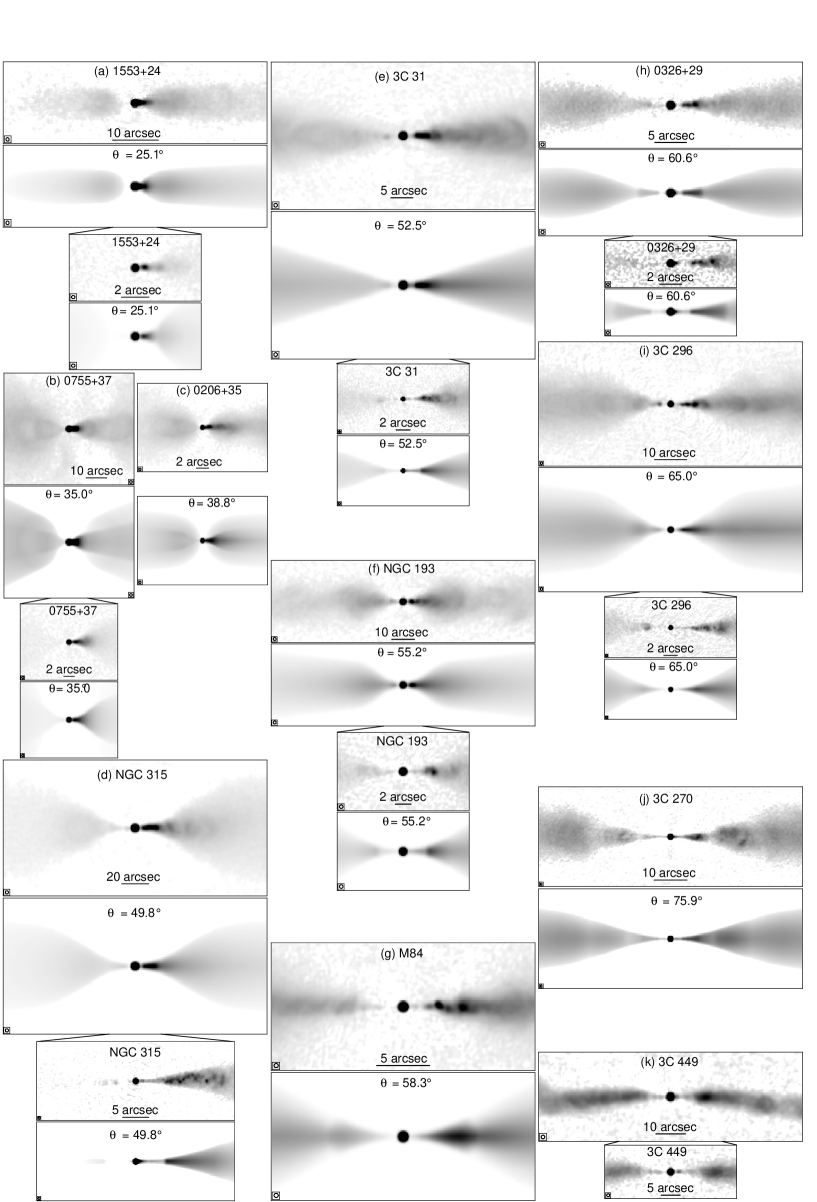
Figure 3: Comparison between observed and model total-intensity images. The plots are arranged in pairs. The upper and lower panels of each pair show the observed image (labelled with the source name) and the model image (with the fitted value of $\theta$), respectively. The angular scale is indicated by a labelled bar on the upper panel and the FWHM of the beam by a circle in one of the lower corners. If two image resolutions were used, then the comparison at high resolution is shown below that at low resolution with the relative areas indicated. The panels are in order of increasing angle to the line of sight, $\theta$. No model is shown for 3C 449 (panel k). Field sizes, grey-scale ranges and resolutions are all given in Table 2.

Figure 4: Comparison between observed and model images of the degree of polarization, $p=P/I$, in the range 0 – 0.7 as indicated by the labelled wedge. The layout is identical to that in Fig. 3. The observed values of $P$ have been corrected for Ricean bias (Wardle & Kronberg, 1974). The observed and model images are both blanked (grey) wherever $I<5\sigma_{I}$ ($\sigma_{I}$ is the off-source noise level). There are systematic errors in $p$ around the edges of the structure of 0755+37 (panel b), where the signal-to-noise ratio is low and there are large uncertainties in lobe subtraction.

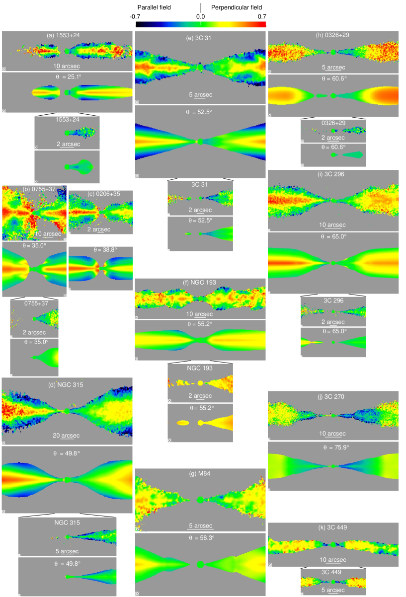
Figure 5: Comparison between observed and model images of the ratio $Q/I$ in the range $-0.7$ to 0.7 as indicated by the labelled wedge. The layout is identical to that in Fig. 3. The observed and model images are both blanked (grey) wherever $I<5\sigma_{I}$ ($\sigma_{I}$ is the off-source noise level).

Detailed comparisons between data and model fits (including profiles along and transverse to the jet axes) are presented elsewhere (Laing & Bridle, 2002a; Canvin & Laing, 2004; Canvin et al., 2005; Laing et al., 2006b; Laing & Bridle, 2012, Laing & Bridle, in preparation; Laing et al., in preparation). Here, we show images which summarize the results in such a way as to emphasize general features and trends with inclination (Figs 3 – 5 and 27). In all of the plots, the radio core component is at the centre and the brighter (approaching) jet is to the right. Panels (a) – (j) show model and observed images and are arranged in order of increasing fitted angle to the line of sight, $\theta$, which is indicated on the model panels. The final panel (k) shows the observations only for 3C 449. Leaving aside the small-scale structure which we cannot model, the overall quality of the fits is extremely good and a clear pattern of inclination-dependent features has emerged.

Fig. 3 shows the observed and model total-intensity images over identical brightness ranges (the peak intensities are listed in Table 2). All of the sources show initial geometrical flaring followed by recollimation to a uniformly expanding flow. The location of the brightness flaring point is clear at high resolution in all of the main jets. The jet/counter-jet ratio decreases monotonically with distance from the brightness flaring point, often reaching $I_{\rm j}/I_{\rm cj}\approx 1$ at the edges of the plots, as expected for flows decelerating to subrelativistic velocities. Our model fits require similar velocities at the brightness flaring point for all of the sources (Section 5.2), so the jet/counter-jet ratio there is anticorrelated with angle, as is evident from the sequence of plots. This sequence is completed by 3C 449, whose jet structure is highly symmetrical, and which we believe to have $\theta\approx 90^{\circ}$. The transverse intensity profiles also differ systematically, in the sense they tend to be centrally peaked in the main jets but flatter or even centre-darkened in the counter-jets. The outer isophotes on both sides of the nucleus are quite symmetrical, even if the on-axis brightness distributions are not. These phenomena are naturally interpreted as the effects of transverse velocity gradients: the flow is faster on-axis than at the jet boundaries.

In Fig. 4, we present images of the degree of polarization, $p=P/I$, in the range $0\leq p\leq 0.7$, with identical blanking for the observed and model images. In the coordinate system of Section 3.2, where the zero-point of ${\mn@boldsymbol{E}}$-vector position angle is the jet axis, the linear polarization is dominated by the $Q$ Stokes parameter: if the jets are approximately cylindrical, then the polarization ${\mn@boldsymbol{E}}$-vectors are either parallel or perpendicular to the axis, and $U\approx 0$. A clearer picture of the polarization asymmetries is therefore provided by images of $Q/I$, which we show in the range $-0.7\leq Q/I\leq 0.7$ in Fig. 5. Parallel and perpendicular apparent magnetic fields have $Q/I<0$ and $Q/I>0$, respectively. A full description of the linear polarization state requires all three Stokes parameters, and this is particularly important where $U$ and $Q$ are both significant, for example at the edges of the flaring regions: we display vectors with lengths proportional to $p$ and directions along the apparent magnetic field in Fig. 27. The vector plots have a similar format to Figs 3 – 5, but are on larger scales.

All of the modelled sources show a common pattern of asymmetry in $p$ which correlates with that seen in total intensity (Fig. 4). In the main (approaching) jet bases, $p$ is low close to the AGN on the jet axis, drops to $p\approx 0$ and then rises gradually with distance. It is larger at the same distance from the nucleus in the counter-jet, increasing monotonically with distance. $p$ is high on the jet axis (particularly in the counter-jet) and at the edges of both jets, dropping to low values at intermediate radii. In $Q/I$ (Fig. 5), this characteristic pattern becomes clearer. On-axis in the main jet, $Q/I$ is negative close to the nucleus, goes through 0 and becomes positive farther out. This is the well-known transition from longitudinal to transverse apparent field in the approaching jet bases of FR I sources (Bridle, 1984). The counter-jets behave differently: $Q/I$ is generally $>$0 everywhere on-axis (predominantly perpendicular apparent field), with a magnitude that increases with distance. $Q/I$ tends to be negative (longitudinal apparent field) at the edges of both jets, but particularly on the counter-jet side. These patterns are also clear in the vector plots (Fig. 27), where high degrees of polarization and close alignment of the field vectors with the outer boundary at the edges of the jets (particularly in the flaring region) are often evident.

The asymmetries in linear polarization at the bases of the jets are perfectly correlated with those in total intensity and well fitted by our models, consistent with the hypothesis that both are caused by relativistic aberration. 3C 449 is symmetrical in polarization structure, just as it is in total intensity, consistent with expectations for a source close to the plane of the sky.

At larger distances from the AGN, the pattern of transverse apparent field on-axis and longitudinal field at the edges persists in most of the modelled sources, but (like the total intensity) becomes more symmetrical as the jets decelerate. 0326+39 shows a different polarization distribution, with less transverse variation in $Q/I$ and no evidence for a parallel-field edge, indicating a qualitatively different intrinsic field configuration (Figs 5h and 27h).

The polarization images for 3C 270 show large deviations from axisymmetry, and the fits are therefore poor (Appendix C).

5 Model results

The values of the fitted parameters, their estimated errors and the angle range $\Delta\theta$ are tabulated in Appendix E.

In order to compare the sources, we show plots of outer isophotes, velocity, emissivity function and fractional field components over fixed multiples of the recollimation distance, $r_{0}$, in Figs 6 – 11, below.

5.1 Geometry

Fig. 6(a) shows the profiles of the model jet boundaries to the same linear scale, emphasizing that the majority of sources have recollimation distances, $r_{0}$, between 5 and 15 kpc. The conspicuous outliers are M 84 ($r_{0}=1.8$ kpc; the closest and least luminous of the sample members) and NGC 315 ($r_{0}=35$ kpc). The shapes of the geometrically flaring regions are remarkably similar: Fig 6(b) shows the outer boundaries of the jet outflows scaled to the same value of $r_{0}$. The ratio of width to length of the flaring region, $x_{0}/r_{0}$, has a mean value of 0.29 with an rms of 0.06. The majority of the outer jets have half-opening angles, $\xi_{0}$ in the range $2^{\circ}$ – $10^{\circ}$, the two exceptions with $\theta>10^{\circ}$ being 3C 31 and M 84 (Fig. 6c).

Figure 6: Plots of model jet geometry. (a) The outer boundaries of the model jet outflows in the plane containing the jet axis, drawn to the same linear scale and ordered by recollimation distance, $r_{0}$. The flaring and outer regions are plotted as full and dotted lines, respectively. (b) The outer boundaries (full lines), scaled to the same value of the recollimation distance, $r_{0}$. The dashed curves represent the boundaries between outer and flaring regions. (c) Histogram of the half-opening angle of the outer region, $\xi_{0}$.

5.2 Velocity

The model velocity fields for the jet outflows are plotted in Fig. 7(a) – (j) and longitudinal profiles on-axis and at the edges of the jets are shown in Fig. 7(k) and (l), respectively. The on-axis velocity first becomes well determined just downstream of the brightness flaring point, where it has a mean value $\langle\beta_{1}\rangle=0.81$, with a rms of 0.08 (compared with 0.06 expected from the estimated errors alone). All sources show unambiguous evidence for deceleration. There is usually a short region beyond the flaring point over which the velocity field shows no detectable variation with distance, although deceleration begins almost immediately in NGC 193. Rapid deceleration occurs over a limited range of distance: in most cases, the evidence for further deceleration or acceleration at $r>r_{v0}$ is weak, and the velocity is consistent with a constant value. In particular, the apparent accelerations in 0326+39 and 1553+24 are marginally significant (Canvin & Laing, 2004): minimal models with $\beta_{f}=\beta_{0}$ provide almost as good a fit (Table 7) and there are indications from the emissivity function evolution that they are physically more plausible (Section 8.4). In 3C 270, the velocity is consistent with 0 for $r>r_{v0}$ and in M 84 it is undetermined there. Only 3C 31 decelerates significantly after recollimation.

The sources can be divided into two groups by on-axis speed after deceleration, $\beta_{0}$. Four (3C 31, NGC 315, 0206+35 and 3C 296) have $\beta_{0}>0.5$. The remaining sources have $\beta_{0}<0.3$.

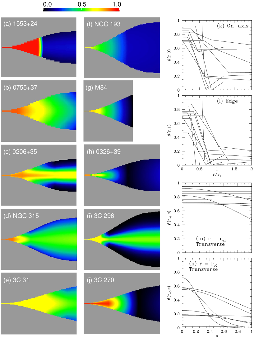
Figure 7: (a) – (j): false-colour plots of the model velocity fields, in the range $0\leq\beta\leq 1$. The maximum plot width is scaled to a distance of $r_{0}/0.85$ from the nucleus (a smaller region is plotted for M 84). The backflow components of the models for 0755+37 and 0206+35 are not shown. (k) and (l): longitudinal velocity profiles for all of the modelled sources. The distance coordinate, $r$, is normalized by the recollimation distance, $r_{0}$, and the maximum range is $2r_{0}$. (k) on-axis; (l) edge. (m) and (n): transverse velocity profiles. Velocity is plotted against streamline index $s$ at constant distance $r$. (m) profile at the start of deceleration, $\beta(r_{v1},s)$; (n) profile at the end of rapid deceleration, $\beta(r_{v0},s)$. $\beta_{0}=0$ for M 84 and 3C 270 and 0.02 for 0326+39. Even though the values of $v_{0}$ are essentially unconstrained for these sources (Table 8), the errors in the transverse profiles are small.

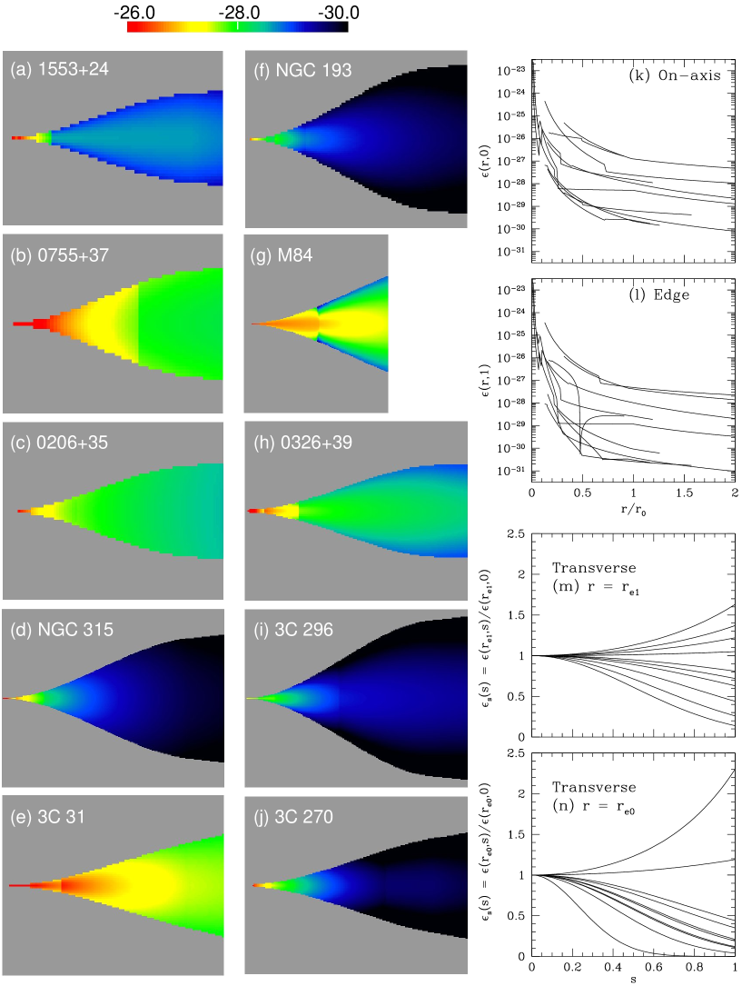
Figure 8: (a) – (j): false-colour plots of the emissivity function $\log\epsilon(r,s)=\log(n_{0}B^{1+\alpha})$ (with $n_{0}$ and $B$ in SI units). The plotted areas are the same as in Fig. 7(a) – (j). (k) and (l): longitudinal profiles of $\epsilon$ for all of the modelled sources. The distance coordinate, $r$, is normalized by the recollimation distance, $r_{0}$. (k) on-axis, $\epsilon(r,0)$; (l) edge $\epsilon(r,1)$. The profiles for emission upstream of the brightness flaring point, $r<r_{e1}$ are only plotted if the exponent $E_{\rm in}$ is well determined. (m) and (n): normalized transverse emissivity function profiles, plotted against streamline index $s$ at constant distance $r$. (m) profile at the brightness flaring point, $\epsilon_{s}(s)=\epsilon(r_{e1},s)/\epsilon(r_{e1},0)$; (n) profile at the end of the high-emissivity region, $\epsilon_{s}(s)=\epsilon(r_{e0},s)/\epsilon(r_{e0},0)$.

At or slightly before the start of rapid deceleration ($r\la r_{v1}$), the transverse velocity variations become well determined. Transverse profiles at $r=r_{v1}$ are plotted in Fig. 7(m). Flat (‘top-hat’) profiles are consistent with the fits for all sources except 0326+39. Profiles in which the velocity increases slightly towards the edges of the jet are not allowed by the fitting software (Section 3.5.2), but would also be consistent with the data in some cases. We see no evidence for any sharp velocity gradient at the jet edge, subject to the limits set by transverse resolution.

Transverse profiles at the end of rapid deceleration, $r=r_{v0}$, are plotted in Fig. 7(n). The normalized transverse velocity profiles clearly evolve with distance from the nucleus in 0206+35, NGC 315, 3C 31 and 3C 296 (where $\beta_{0}>0.5$). There is a hint of a relation between edge velocity and environment for these four sources: the jets in 0206+35 and 3C 296 propagate within lobes and their edge velocities drop rapidly to values consistent with zero whereas those in NGC 315 and 3C 31 ($v_{0}=0.36$ and 0.47, respectively) appear to be in direct contact with the surrounding hot gas. The transverse velocity profiles for 0206+35, NGC 315 and 3C 296 remain well determined beyond $r=r_{v0}$ and do not evolve significantly.

If the on-axis velocity is low, transverse variations in Doppler factor are slight, and the velocity difference between centre and edge is harder to measure, particularly if $\theta$ is large. Three other sources show evidence for transverse velocity gradients, but with larger errors: 1553+24, 0755+37 and 0326+39. The first two have small on-axis velocities $\beta_{0}\approx 0.2$, but low inclinations, so evolution of the profile is still detectable. As mentioned above, 0326+39 is unusual in showing a transverse gradient at $r=r_{v1}$. This persists over the first half of the deceleration region (consistent with the initial value of $v_{1}\approx 0.6$), after which the velocity becomes too low to measure a gradient and $v_{0}$ is unconstrained. The velocity profile of NGC 193 is consistent with a constant value, but with large errors.

Finally, $v_{0}$ is undetermined for M 84 and 3C 270, which decelerate rapidly to speeds at which relativistic aberration is negligible.

To summarize: evolution of the transverse velocity profiles is measured accurately in four cases, and is required in a further two. Relative transverse velocity variations of the same form are not excluded in any of the remaining four sources. The unweighted mean fractional edge velocity after deceleration is $\langle v_{0}\rangle=0.35$ with the three undetermined values excluded, compared with $\langle v_{1}\rangle=0.92$ at its start.

The velocity fields are not well determined between the nucleus and the brightness flaring point (Sections 3.5.5 and  8.7).

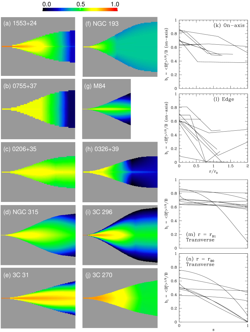
Figure 9: (a) – (j): false-colour plots of the fractional longitudinal component of the magnetic field, $b_{l}=\langle B^{2}_{\rm l}\rangle^{1/2}/B$, in the range 0 – 1. The plotted areas are the same as in Fig. 7. (k) and (l): longitudinal profiles of $b_{l}=\langle B^{2}_{\rm l}\rangle^{1/2}/B$. The distance coordinate, $r$, is normalized by the recollimation distance, $r_{0}$. (k) on-axis; (l) edge. (m) and (n): transverse profiles of $b_{l}=\langle B^{2}_{\rm l}\rangle^{1/2}/B$, plotted against streamline index $s$ at constant distance $r$. (m) profile at the inner fiducial distance, $r_{B1}$; (n) profile at the outer fiducial distance, $r_{B0}$. Profiles are only plotted where the field component fraction has a range of $<$0.5 as deduced from the errors on the field ratios in Table 8.

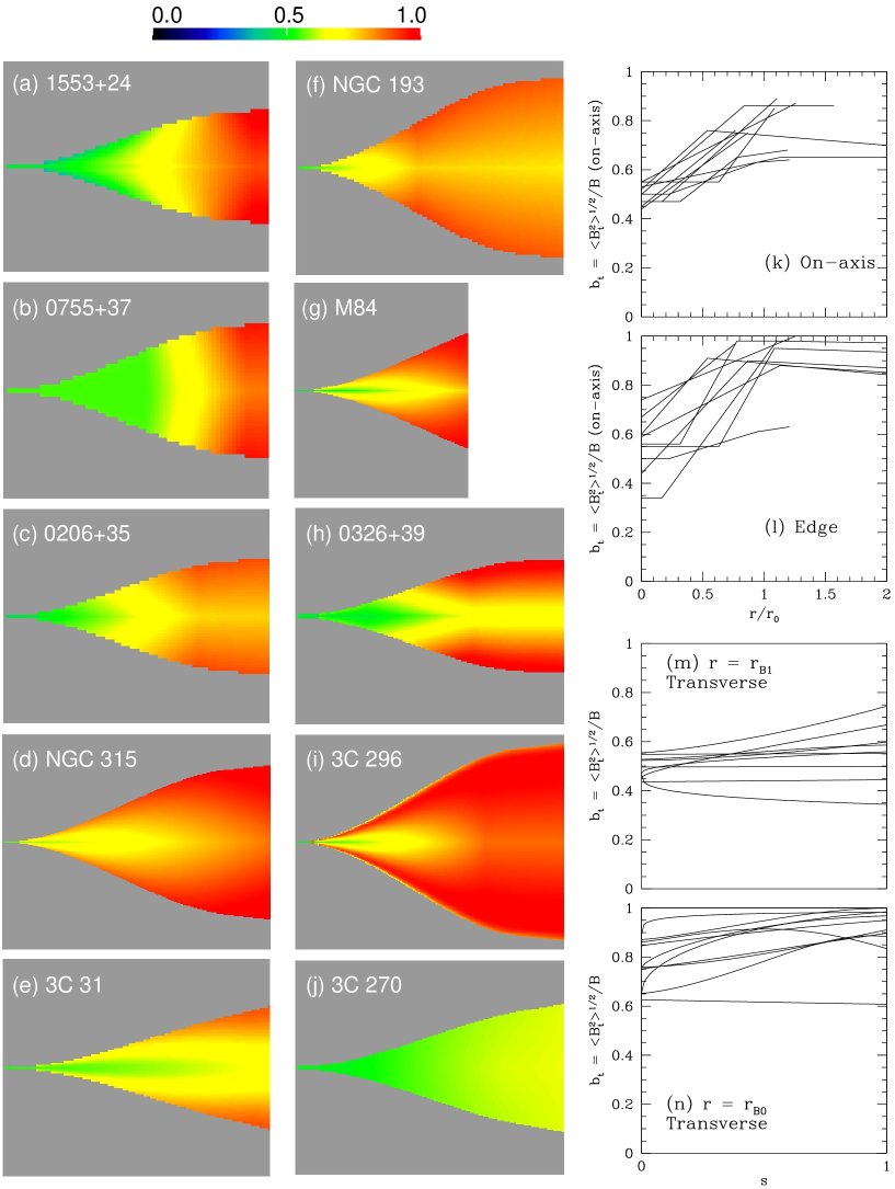
Figure 10: False-colour plots and profiles of the fractional toroidal component of the magnetic field, $b_{t}=\langle B^{2}_{\rm t}\rangle^{1/2}/B$. The layout is identical to that in Fig. 9.

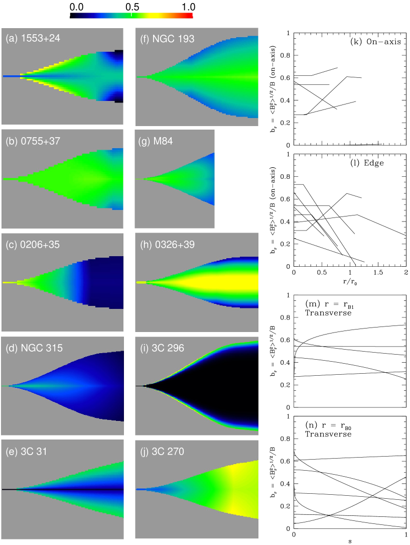
Figure 11: False-colour plots and profiles of the fractional radial component of the magnetic field, $b_{r}=\langle B^{2}_{\rm r}\rangle^{1/2}/B$. The layout is identical to that in Fig. 9.

5.3 Emissivity function

Model distributions for the emissivity function $\epsilon(r,s)=n_{0}B^{1+\alpha}$ are plotted in Fig. 8(a) – (j) and longitudinal profiles on-axis and at the edges of the jets are shown in Fig. 8(k) and (l), respectively.

The emissivity structure up to the brightness flaring point is not well constrained (Section 3.5.5). Subject to our assumption of constant velocity at $r\leq r_{v1}$, an increase of emissivity function from upstream to downstream of the flaring point is required by the data for 1553+24, NGC 315, 3C 31, NGC 193 and 0326+39. In the remaining cases, the emissivity function is consistent with being continuous across the flaring point, but with a change of slope: there will be a marked increase in brightness purely as a result of the rapid spreading of the jet in this vicinity provided that the emissivity function fall-off is not too steep.

The end of the high-emissivity region is usually marked by one or both of a discontinuous drop in emissivity function ($g_{0}<1$; 1553+24, 0755+37, NGC 315, 0326+39, 3C 296) or a significant flattening in the slope of the longitudinal emissivity function profile ($E_{\rm out}<E_{\rm mid}$; 1553+24, 0755+37, 0206+35, 3C 31, NGC 193, 0326+39).

There is a general tendency for the power-law slope of the emissivity function variation to flatten with distance from the nucleus (Figs 8k and l). In three cases ($E_{\rm out}$ for 1553+24 and 3C 270; $E_{\rm mid}$ for M 84), this progression is interrupted by short regions of roughly constant emissivity function. Values of the power-law slope after recollimation are between 0.9 and 2.2.

Figs 8(m) and (n) illustrate the tendency for the transverse emissivity function profile to evolve from uniform (or perhaps even slightly limb-brightened in some cases) to centrally peaked (0206+35 and 0755+37 remain uniform, with even a hint of a thin layer of enhanced emission at the boundary between outflow and backflow). The (unweighted) mean values of the fractional edge emissivity function are $\langle e_{1}\rangle=0.82$ at the brightness flaring point and $\langle e_{0}\rangle=0.50$ at the end of the high-emissivity region.

5.4 Magnetic field structure

False-colour plots of the fractional longitudinal, toroidal and radial field components, $b_{\rm l}=\langle B^{2}_{\rm l}\rangle^{1/2}/B$, $b_{\rm t}=\langle B^{2}_{\rm t}\rangle^{1/2}/B$ and $b_{\rm r}=\langle B^{2}_{\rm r}\rangle^{1/2}/B$, are plotted in panels (a) – (j) of Figs. 9 – 11, respectively. Longitudinal and transverse profiles are shown in panels (k) – (n) of the same Figures. The errors in the field-component ratios (particularly the radial/toroidal ratio $j$) can be large, and there are real differences between sources. Nevertheless, some clear trends emerge. We quantify these using values of the fractional field components $\langle b_{\rm l}\rangle$, $\langle b_{\rm t}\rangle$ and $\langle b_{\rm r}\rangle$ computed from the error-weighted mean field ratios at the fiducial distances.

1. The largest single field component close to the AGN is longitudinal; the toroidal component dominates at large distances.

2. The radial component does not show any obvious systematic trends and is usually the weakest of the three.

3. Consequently, the images of toroidal and longitudinal field fraction are strikingly anticorrelated, except in a few locations where the radial field is significant (Figs 9 and 10).

4. Close to the nucleus ($r\approx r_{B1}$):

   1. the longitudinal component tends to be slightly stronger than the toroidal component on-axis and the radial component is small: $\langle b_{\rm l}\rangle=0.78$, $\langle b_{\rm t}\rangle=0.55$ and $\langle b_{\rm r}\rangle=0.29$;

   2. the field approaches isotropy at the edges: $\langle b_{\rm l}\rangle=0.62$, $\langle b_{\rm t}\rangle=0.61$ and $\langle b_{\rm r}\rangle=0.50$.

5. At larger distances $r\approx r_{B0}$, the field configuration becomes mostly toroidal.

   1. The toroidal component is always dominant at the edge of the jet: $\langle b_{\rm l}\rangle=0.05$, $\langle b_{\rm t}\rangle=0.97$ and $\langle b_{\rm r}\rangle=0.23$.

   2. It is also usually the largest single component on-axis, although the longitudinal component remains significant: $\langle b_{\rm l}\rangle=0.55$, $\langle b_{\rm t}\rangle=0.80$ and $\langle b_{\rm r}\rangle=0.23$.

   3. 3C 296 and NGC 315 are particularly striking, in that the field is almost purely toroidal over most of their outer jets, with only small longitudinal components on-axis.

6. There is little evidence for further evolution in the field components at larger distances $r>r_{B0}$.

The approximate equality of longitudinal and toroidal field on-axis in the middle of the flaring region is the key to understanding the clear asymmetry in polarization between the main and counter-jets seen in Figs 4 and  5. If the radial component is negligible, $\langle b_{l}\rangle\approx\langle b_{t}\rangle\approx 2^{-1/2}$, so the field forms a two-dimensional sheet with equal components in the two directions. This is the case described by equations (15) – (19). The zero polarization point on the axis of the main jet occurs where $\beta=\cos\theta$ in this approximation. For example, we would expect $p=0$ where $\beta=0.57$ for $\theta=50^{\circ}$, typically in the deceleration region. At the corresponding distance from the AGN in the counter-jet, the degree of polarization would be $p\approx 2p_{0}\cos^{2}\theta/(1+\cos^{4}\theta)\approx 0.5$ with a transverse apparent field (equations 15 and 16). We also expect longitudinal apparent field with $p$ approaching $p_{0}$ at the edges of both jets in this model, again consistent with the observations.

There is one special case in which the radial and toroidal components are similar in magnitude over a significant volume: on-axis in 0326+39 at large distances (Figs 10h and 11h). This part of the jet resembles a two-dimensional field sheet with $\langle B^{2}_{t}\rangle^{1/2}\approx\langle B^{2}_{r}\rangle^{1/2}\gg\langle B^{2}_{l}\rangle^{1/2}$, as described by equations (11) – (14).

6 Consistency tests

6.1 General

There are obvious selection effects in our choice of source: it is hard for us to model jets which are highly projected (in which case slight bends appear amplified) or close to the plane of the sky (so that intrinsic or environmental asymmetries exceed relativistic effects). Our sources are selected from parent samples with random distributions of inclination, but the distribution of orientations we derive is biased in the sense that values of $\theta$ between $\approx$30^∘ and $\approx$65^∘ are over-represented. Our objectives in this section are to test whether the distributions of orientation indicators for our sources are consistent with those of their parent samples – i.e. that the sample members we have not observed are predominantly at higher and lower inclinations – and to look for correlations between the values of $\theta$ we derive and independent measures.

Eight of the 10 modelled sources are drawn from two complete samples, as follows.

B2

Laing et al. (1999) selected a complete sample of 38 nearby FR I radio sources with jets from the B2 catalogue. Of these, we modelled four (0206+35, 0326+39, 0755+37 and 1553+24).

3CRR

In order to define a similar sample starting from the 3CRR catalogue (Laing et al., 1983), we selected FR I sources with kpc-scale jets on at least one side of the nucleus and $z<0.05$, adding NGC 315, which meets the selection criteria on the basis of later flux-density measurements (Mack et al., 1997). We observed and modelled 4 of these (3C 31, NGC 315, M 84 and 3C 296) from a total of 15. 3C 449 is also a member of this sample (3C 270 satisfies the flux-density criterion but is outside the Declination range).

The jet inclinations for sources in these two parent samples are expected to be isotropically distributed to a good approximation, since the emission at the selection frequencies (178 MHz for 3CRR and 408 MHz for B2) should come primarily from slowly moving, extended components such as outer jets, lobes or tails. Deviations from isotropy caused by dependences of the total flux density and angular size on orientation are likely to be slight (post hoc estimates based on our jet models are given by Laing et al. 1999 and Canvin & Laing 2004).

We use three orientation indicators: jet sidedness (i.e. jet/counter-jet intensity ratio; Section 6.2) fractional core flux density (Sections 6.3 and 6.4), and the ratio of Faraday rotation or depolarization (Sections 6.5 and 6.6). The jet/counter-jet ratio is expected to be the most accurate of the three orientation indicators, but is used implicitly in our modelling and thus does not provide an independent test. The core fraction is known to vary with time, but is not used in the model and has a predictable dependence on angle. The Faraday ratio is also independent of the model, but its variations with $\theta$ are determined by the host galaxy environment, in which there is a wide range. We can usefully check the distributions of all three indicators for our modelled sources against those for the parent samples and the correlations of core fraction and Faraday ratio with $\theta$ for the modelled sources alone.

6.2 Jet sidedness distribution

Figure 12: A histogram of the jet/counter-jet ratios at the brightness flaring point, $I_{\rm j}/I_{\rm cj}$, for the 38 sources in the B2 jet sample defined by Laing et al. (1999). The four modelled sources from this sample (for which the inclination range is $25^{\circ}$ to $61^{\circ}$) are hatched and the median value of $I_{\rm j}/I_{\rm cj}$ is indicated by a dotted line.

We deliberately chose to model sources with significant brightness asymmetries (at least 5:1 and more usually $\ga$10:1) in their jet bases. For a single-velocity flow with $\beta=0.81$ (the mean initial velocity we estimate) and $\alpha=0.6$ emitting isotropically in the rest frame, $I_{\rm j}/I_{\rm cj}\geq 5$ corresponds to $\theta\leq 68^{\circ}$ (equation 10), in adequate agreement with our inferred inclination range of $25^{\circ}\leq\theta\leq 76^{\circ}$.

Next, we ask whether the ratios for the modelled sources are consistent with their membership of an isotropic parent sample. A homogeneous set of measurements of the jet/counter-jet ratio at the brightness flaring point is available for the B2 jet sample (Laing et al., 1999) and their distribution is shown in Fig. 12. All of the modelled sources in this sample have ratios above the median, consistent with their derived inclination range of $25^{\circ}-61^{\circ}$.

6.3 Core fraction distribution

A second, widely-used, orientation indicator is the ratio $f$ of radio core to extended flux density (or luminosity) at fixed emitted frequency. The core emission is partially optically thick and comes from the bases of the jets (Blandford & Königl, 1979). A simple model in which there is a constant intrinsic ratio of core to extended flux density (or luminosity) and the parsec-scale emission comes from a pair of antiparallel jets with velocity $\beta_{\rm c}$ and spectral index $\alpha_{\rm c}$ predicts

$$f = f_{0}\frac{(1-\beta_{\rm c}\cos\theta)^{-(2+\alpha_{\rm c})}+(1+\beta_{\rm c}\cos\theta)^{-(2+\alpha_{\rm c})}}{(1-\beta_{\rm c}/2)^{-(2+\alpha_{\rm c})}+(1+\beta_{\rm c}/2)^{-(2+\alpha_{\rm c})}}$$ (24)

again assuming isotropic emission in the rest frame. $f_{0}$ is the core fraction at $\theta=60\degr$ (the median value for an isotropic sample).

One potential complication is that the relation between core and extended luminosity is non-linear (Giovannini et al., 1988; de Ruiter et al., 1990). For this reason, Laing et al. (1999) defined an alternative orientation indicator, the normalized core power, $P_{\rm cn}$. This is the ratio of $f$ to its median value at given extended luminosity. Given that the sample used to establish the slope of the median relation has a much larger luminosity range than we consider here, is dominated by types of source other than twin jets and includes powerful FR II sources, it is not clear whether this normalization is valid for our sample. We therefore prefer to use $f$ rather than $P_{\rm cn}$. The range of extended luminosity for the sources in this paper is a factor of $\approx$40, with the majority having $\log(P_{\rm ext}/{\rm WHz}^{-1})$ close to the median value of 24.3 (Table 2), so the normalization will not, in any case, affect our results significantly.

In Fig. 13, we show the distributions of the core fraction $f$ at 1.4 GHz emitted frequency for the 3CRR and B2 jet samples, with the modelled sources and 3C 449 indicated. For the modelled sources, the inclination ranges are $50^{\circ}<\theta<65^{\circ}$ (3CRR) and $25^{\circ}<\theta<61^{\circ}$ (B2); we expect $\theta\approx 90^{\circ}$ for 3C 449. We therefore predict core fractions from just below to significantly above the median for the modelled sources and close to the lower end of the distribution for 3C 449. The observed and predicted distributions are reasonably consistent, especially considering the possibility of dispersion in the intrinsic core fraction.

Figure 13: (a) and (b): histograms of core/extended flux-density ratio, $f$, for the B2 and 3CRR samples. The modelled sources are hatched and the dotted line indicates the median ratio for the sample. (a) 3CRR sample (Laing et al., 1983). The four modelled sources have estimated inclinations between $50^{\circ}$ and $65^{\circ}$. 3C 449, for which we estimate $\theta\approx 90^{\circ}$, is shaded black. (b) B2 jet sample (Laing et al., 1999). The inclination range for the modelled sources is $25^{\circ}$ to $61^{\circ}$.

Figure 14: (a) A plot of the ratio, $f$, of core to extended flux density at 1.4 GHz rest frequency against $\theta$ for the sources in our sample. The full curve is the expected relation if the core emission comes from a pair of antiparallel jets with a spectral index of $-0.2$ (the mean for our sample), the best-fitting bulk speed, $\beta_{\rm c}=0.98$, and $f_{0}=0.0195$ (equation 24). The dotted lines represent the median values of $\theta$ ($=60^{\circ}$) and core flux density ratio, $f_{0}$, for an isotropic sample. (b) A plot of core luminosity, $P_{\rm c}$ against extended luminosity $P_{\rm ext}$, both at an emitted frequency of 1.4 GHz. The best-fitting linear relation is shown. (c) As (b), but with the core luminosity $P^{\prime}_{\rm c}$ corrected for beaming using equation (25). In all three panels, data for the modelled sources are plotted as filled squares. The filled circles represent 3C 449. This source, which we take to have $\theta=90^{\circ}$, was not included in any of the fits.

6.4 Correlation of core fraction with inclination

We plot the relation between inclination and core fraction at an emitted frequency of 1.4 GHz in Fig. 14(a). There is a clear anticorrelation (significant at the 99.8% level according to the Spearman rank test).

The simple model of equation (24) with $\alpha_{\rm c}=-0.2$ (the median for the sample) gives a reasonable fit to the relation for any value of core velocity $\beta_{\rm c}\ga 0.94$. Fig. 14(a) shows an example for the best fit, $\beta_{\rm c}=0.98$ ($\Gamma_{\rm c}=4.8$). The rms scatter in $\log f_{0}$ is 0.26 for this speed. For comparison, Laing et al. (1999) derived $\beta_{\rm c}=0.91\pm 0.05$ from a similar analysis of the relation between core fraction and the jet/counter-jet intensity ratio at the brightness flaring point for the full B2 jet sample, but with a larger scatter of 0.45 in $\log f_{0}$. 3C 449 has a lower value of $f$ than any of the modelled sources, consistent with the expected large angle to the line of sight (we plot it with $\theta=90^{\circ}$ in Fig. 14, but did not use it in the fit).

It is of interest to see how much the scatter in the relation between core and extended luminosity is reduced by fitting out the dependence on inclination in this way. Fig. 14(b) shows a plot of core luminosity, $P_{\rm c}$, against extended luminosity, $P_{\rm ext}$. We have corrected $P_{\rm c}$ to luminosity in the rest frame of the emitting material using the same assumptions as in equation (24). The resulting quantity, $P^{\prime}_{\rm c}$ is given by

$$P^{\prime}_{\rm c} = \frac{2\Gamma_{\rm c}^{2+\alpha_{\rm c}}P_{\rm c}}{(1-\beta_{\rm c}\cos\theta)^{-(2+\alpha_{\rm c})}+(1+\beta_{\rm c}\cos\theta)^{-(2+\alpha_{\rm c})}}$$ (25)

and is plotted against $P_{\rm ext}$ in Fig. 14(c). The relations between core and extended luminosity both before and after correction for Doppler boosting are consistent with our assumption of constant intrinsic ratio. The correction reduces the rms dispersion about the best-fitting linear relation from 0.43 for $\log P_{\rm c}$ to 0.20 for $\log P^{\prime}_{\rm c}$. The best fit for the core luminosity in the rest frame is $P^{\prime}_{\rm c}=0.16P_{\rm ext}$ for a frequency of 1.4 GHz. The implication for the type of source we model is that the rest-frame emission produced on parsec scales (which is known to vary on time-scales of years) is surprisingly well correlated with emission extending in some cases to enormous distances and which is presumably built up over the entire source lifetime.

6.5 Depolarization ratio distribution

The lobe containing the approaching jet will be seen through less magnetoionic material associated with the host galaxy and will therefore show lower fluctuations in foreground Faraday rotation than the receding lobe (Laing, 1988). The degree of polarization integrated over the approaching lobe therefore decreases less rapidly with increasing wavelength in the approaching lobe. We define the average depolarization between two frequencies DP = $<p(\nu_{\rm low})/p(\nu_{\rm high})>$.

Figure 15: Histogram of depolarization ratio, DP_j/DP_cj for the sample defined by Morganti et al. (1997). DP is the ratio of scalar mean degrees of polarization at 1.4 and 4.9 GHz, so a smaller value of DP corresponds to heavier Faraday depolarization. DP_j and DP_cj refer to the lobes containing the brighter and fainter jets, respectively. The three sources in common with this study, 0206+35, 0755+37 and 1553+24, are shown hatched. The vertical dotted line indicates DP${}_{\rm j}=$ DP_cj.

Measurements of the ratios of the mean scalar degrees of polarization at frequencies of 4.9 and 1.4 GHz for the lobes of 37 sources from the B2 sample were presented by Morganti et al. (1997). They confirmed the strong tendency for the lobe containing the brighter jet to be less depolarized, and showed that this is due primarily to sources with one-sided jet bases (or, almost equivalently, bright cores). Fig. 15 shows a histogram of depolarization ratio from Morganti et al. (1997). The three sources in common with this study (0206+35, 0755+37 and 1553+24) are indicated. They have DP_j/DP${}_{\rm cj}\ga 1$, as expected.

6.6 Faraday rotation asymmetry

A more direct measure of Faraday rotation fluctuations is the rms dispersion in RM across a lobe, $\sigma_{\rm RM}$, determined at high spatial resolution. We have published high-quality RM images for eight out of 11 of the sources discussed in this paper. In addition, we made a two-frequency RM image for NGC 193 from observations at 4.9 and 1.365 GHz (Laing et al., 2011). For nine sources, we could therefore derive $\sigma_{\rm RM}$ across the main and counter-jet lobes with good sampling at high resolution. $\sigma_{\rm RM}$ is a more sensitive measure of foreground Faraday rotation than depolarization and allows us to probe much smaller Faraday depths. We evaluated it over all unblanked pixels, making a first-order correction for fitting error to avoid positive bias. The image resolutions and values of $\sigma_{\rm RM}$ are given in Table 3, along with references to the observations and data reduction.

In Fig. 16(a), we plot $\sigma_{\rm RM}$ for the main and counter-jets against each other and in Fig. 16(b), we plot their ratio against inclination. There is a significant asymmetry, in the sense that $\sigma_{\rm RM,j}<\sigma_{\rm RM,cj}$, for $\theta\la 55^{\circ}$ and the ratio is very close to unity for larger angles to the line of sight. There are no examples where $\sigma_{\rm RM,j}$ is significantly larger than $\sigma_{\rm RM,cj}$. The significance of the correlation between $\sigma_{\rm RM,j}/\sigma_{\rm RM,cj}$ and $\theta$ is 97% according to the Spearman rank test.

This result, and the earlier measurements of depolarization asymmetry for the B2 sample (Morganti et al., 1997), are qualitatively consistent with a simple picture in which the variations of Faraday depth across the brightness distributions are produced by roughly spherical distributions of ionized gas containing fluctuating magnetic fields. Profiles of $\sigma_{\rm RM}$ for spherically-symmetric model gas density profiles and power-law dependences of field strength on density indeed show that significant asymmetries can be produced, particularly for $\theta\la 50^{\circ}$ (e.g. Garrington & Conway 1991; Laing et al. 2008b). We note a number of complications, however.

1. The expansion of radio sources into the surrounding hot gas is expected to cause local increases in density and field strength, particularly if the expansion is supersonic (Huarte-Espinosa et al., 2011); shells of denser gas are indeed observed around the lobes of M 84 (Finoguenov et al., 2008).

2. The present sample includes three examples of highly ordered RM distributions which must be affected by interactions between the sources and their local environments (0206+35, M 84 and 3C 270; Guidetti et al., 2011).

3. Even for sources with chaotic RM distributions which might plausibly originate from undisturbed plasma, it is necessary to take account of that fact that the relativistic particles evacuate cavities in the surrounding hot gas, causing deviations from spherical symmetry (e.g. Laing et al. 2008b).

4. There is a wide variation in measured external density profile and in the size of the radio structure compared with the core radius of the surrounding hot gas.

Nevertheless, our results are fully consistent with the idea that the Faraday rotation is produced by distributed, local foreground plasma. A difference between sources at $\theta<55^{\circ}$ (which show significant side-to-side differences) and those with $\theta>55^{\circ}$ (which do not) is apparent from Fig. 16. Such a discontinuity could be produced by the type of cavity model developed by Laing et al. (2008b), but observations of a larger sample would be needed to establish the robustness of the result.

Table 3: Rotation measure rms, $\sigma_{\rm RM}$, for the lobes associated with the main (approaching) and counter (receding) jets. (1) Source name; (2) angle to the line of sight, $\theta$, in deg; (3) resolution (FWHM, in arcsec); (4) rms rotation measure for the main jet lobe, in rad m^-2; (5) as (4), but for the counter-jet lobe; (6) reference.

Source	$\theta$	FWHM	$\sigma_{\rm RM,j}$	$\sigma_{\rm RM,cj}$	Reference
	(deg)	(arcsec)	(rad m-2)
0755+37	35.0	1.3	4.3	6.2	3
0206+35	38.8	1.2	15.6	22.9	2
NGC 315	49.8	5.5	1.6	3.0	5
3C 31	52.5	1.5	12.0	37.0	6
NGC 193	55.2	1.6	2.3	2.7	7
M 84	58.3	1.65	11.7	11.5	2
3C 296	65.0	1.5	7.0	7.6	4
3C 270	75.9	1.65	8.8	8.3	8
3C 449	90.0	1.25	30.9	34.2	1

References: (1) Guidetti et al. (2010); (2) Guidetti et al. (2011); (3) Guidetti et al. (2012); (4) Laing et al. (2006b); (5) Laing et al. (2006a); (6) Laing et al. (2008b); (7) Laing et al. (2011); (8) Laing et al. (in preparation).

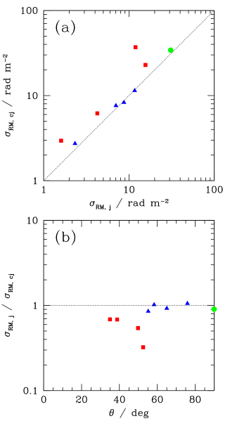
Figure 16: (a) A plot of the rms rotation measure for the counter-jet lobe, $\sigma_{\rm RM,cj}$, against that for the main jet lobe, $\sigma_{\rm RM,j}$. (b) The ratio $\sigma_{\rm RM,j}/\sigma_{\rm RM,cj}$ plotted against $\theta$. In both panels, the points are coded by angle to the line of sight. Red squares: $\theta<55^{\circ}$; blue triangles: $55^{\circ}<\theta<90^{\circ}$; green circles: $\theta\approx 90^{\circ}$ (3C 449). The dotted lines represent $\sigma_{\rm RM,j}=\sigma_{\rm RM,cj}$.

7 Intrinsic asymmetries

We have shown that symmetrical, relativistic jet models can fit the observed brightness and polarization distributions very well, and that their use yields similar values for many of the physical parameters in all cases that we have studied. We are confident that relativistic aberration dominates close to the AGN and that our derived physical parameters are most reliable there. It is obvious, however, that the bending and asymmetric morphologies of FR I jets on much larger scales are inconsistent with the hypothesis of continuing symmetrical flow on those scales and that environmental effects eventually dominate. We have therefore restricted our modelling to the inner jet regions (specifically, where bends in the jets are slight) and have ignored very bent sources completely. The jets are unlikely to be perfectly symmetrical even where they form and our criteria for selecting the regions to model are inevitably somewhat subjective.

For these reasons, we now attempt to quantify the effects of intrinsic side-to-side differences on our results. It is difficult to be definitive without a physical model for the deviations from intrinsic symmetry (which could in principle affect any combination of geometry, emissivity function, velocity or field structure in complicated ways). We have therefore chosen to analyse three representative examples, in which the deviations are only in one of velocity, rest-frame emissivity function or field ordering.

We constructed a base model with representative parameters, including: $\beta_{1}=0.8$, $v_{1}=1.0$, $\beta_{0}=0.32$ and $v_{0}=0.5$ (equivalent to an emissivity-weighted average of $\beta=0.24$ at $r\geq r_{v0}$), with $r_{v1}$ and $r_{v0}$ corresponding to 1.8 and 5.0 kpc on a model grid of 10 kpc (all in projection). We took four representative angles to the line of sight, $\theta=30^{\circ}$, $45^{\circ}$, $60^{\circ}$ and $75^{\circ}$.

7.1 Velocity

We modified the base model by multiplying all of the velocities on one side of the nucleus by a constant factor, made model images and then fit to them using our standard procedures. As expected, a velocity asymmetry of this type is fit primarily by changes in a combination of the on-axis velocities $\beta_{1}$ and $\beta_{0}$, the fractional edge velocities $v_{1}$ and $v_{0}$, and the angle to the line of sight, $\theta$. The fitted value of $\theta$ is biased in the obvious sense: it is underestimated if the approaching jet is faster and overestimated if it is slower. For a 20% difference in velocity, the maximum error in $\theta$ ranges from 1$\aas@@fstack{\circ}$6 at $\theta=30^{\circ}$ to 2$\aas@@fstack{\circ}$4 at $\theta=70^{\circ}$. The fitted velocities $\beta_{1}$ and $\beta_{0}$ typically lie mid-way between the mean of the new main and counter-jet velocities and the values for the base model, so the error on the true mean velocity is about 5% for a 20% asymmetry, as is the error on $v_{0}$ and $v_{1}$.

We conclude that the fits are robust to asymmetries in velocity, with errors typically at the 5% level for a 20% asymmetry, comparable with our estimated errors.

7.2 Emissivity function

This example is perhaps the most interesting, because we can constrain the intrinsic emissivity function ratio between the two jets from the statistics of reversals in sidedness in a sample of sources. Suppose that all jets have a constant intrinsic sidedness ratio $R_{\rm int}$, but that they have identical velocity fields. Provided that the velocity is sufficiently high near the nucleus, relativistic effects will dominate there except for jets which are very close to the plane of the sky, so we will identify the near side correctly in almost all cases. Farther from the nucleus, where the jets have decelerated, we will observe reversals in the observed sidedness if the approaching jet is the intrinsically fainter one and the angle to the line of sight is sufficiently large. Suppose that the jets decelerate from $\beta=\beta_{1}$ to $\beta=\beta_{0}$. Then we will observe reversals for angles in the range $\theta_{1}>\theta>\theta_{0}$, where

$$R_{\rm int} = \left[\frac{1+\beta_{1}\cos\theta_{1}}{1-\beta_{1}\cos\theta_{1}}\right]^{2+\alpha}$$ (26)

$$= \left[\frac{1+\beta_{0}\cos\theta_{0}}{1-\beta_{0}\cos\theta_{0}}\right]^{2+\alpha}$$

assuming isotropic emission in the rest frame (equation 10). The probability of observing reversals in an isotropic sample is then

$$f_{\rm rev} = (\cos\theta_{0}-\cos\theta_{1})/2$$ (27)

and the corresponding intrinsic sidedness ratio is

$$R_{\rm int} = \left[\frac{1/\beta_{0}-1/\beta_{1}+2f_{\rm rev}}{1/\beta_{0}-1/\beta_{1}-2f_{\rm rev}}\right]^{2+\alpha}.$$ (28)

If $\theta>\theta_{1}$ and the receding jet is intrinsically brighter (probability $\cos\theta_{1}/2$), then it will appear brighter at all distances from the nucleus and might be identified as the approaching jet. The jet/counter-jet sidedness ratio will appear to increase with distance from the nucleus in this case, however.

For an alternative model in which the jets are intrinsically symmetrical at the base but develop an intrinsic asymmetry after deceleration, the ratio is

$$R_{\rm int} = \left[\frac{1/\beta_{0}+2f_{\rm rev}}{1/\beta_{0}-2f_{\rm rev}}\right]^{2+\alpha}.$$ (29)

For the B2 jet sample, we have measurements of sidedness ratio at a projected distance of 14.3 kpc from the nucleus for 25 sources, of which 2 show reversals in sidedness compared to the brightness flaring point (Laing et al., 1999, Fig. 6c), so $f_{\rm rev}=0.08$. The mean ratios at 14.3 kpc (averaged over all sources and also subdivided by fractional core flux density) are consistent with $\beta_{0}\approx 0.24$ for isotropic emission: this is an emissivity-weighted average across the jets, and therefore corresponds to a somewhat higher on-axis velocity, as in our base model. For an initial velocity $\beta_{1}=0.8$ and a model with a constant intrinsic asymmetry, we find $R_{\rm int}\approx 1.3$ (equation 28); if the jets are initially symmetrical, then $R_{\rm int}\approx 1.2$ (equation 29). We use the latter model, since we have found no cases of sidedness ratio increasing with distance in the B2 jet sample (although only $\approx 1/25$ would in any case be expected). The sample size is small and the selection criteria for the B2 jet sample include a wider variety of source types than we consider here, so our estimate is very approximate. Nevertheless, it does indicate that intrinsic emissivity function variations are fairly small on the typical scales we model.

In order to test the effects of such an asymmetry on our derived parameters, we started with the symmetrical base model and multiplied the emissivities of one of the jets by a factor increasing linearly from 1 at the nucleus to 1.2 at $r=r_{0}$ and thereafter remaining constant. The principal systematic errors are in the angle to the line of sight, $\theta$ and the velocity variables after deceleration, $\beta_{0}$ and $v_{0}$. These are in the obvious sense that sources with the intrinsically brighter jet on the near side are fit as being closer to the line of sight and/or faster, the deviations increasing with $\theta$. If the intrinsically brighter jet is on the far side, the effects are in the opposite sense. Errors in $\theta$ range from $\approx$1°at $\theta=30\degr$ to $\approx$4°at $\theta=75\degr$; in $\beta_{0}$ from 0.04 to 0.09 and in $v_{0}$ from 0.04 to 0.08. With the assumed form of variation in asymmetry, the errors in quantities measured at the flaring point are negligible. There are also errors at the 10% level in the edge emissivities and radial/toroidal field ratios.

Emissivity function variations at the level we have simulated will limit our ability to model jets with $\theta\ga 75\degr$, but are comparable with or less than other sources of error for lower inclinations.

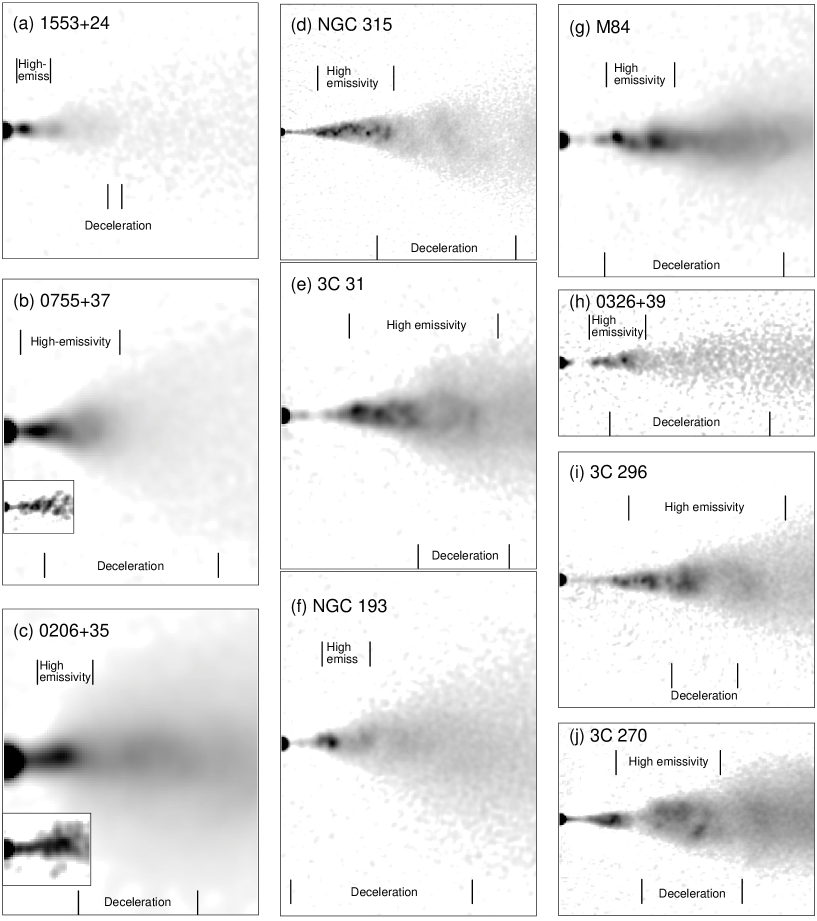
Figure 17: Grey-scale plots of total intensity for the main jet bases, showing the locations of the high-emissivity and rapid deceleration zones. The main panels are VLA images at the highest available resolution (Table 2); the inserts in panels (b) and (c) are MERLIN images (Laing et al., 2011), plotted on the same scale.

7.3 Field ordering

Finally, we checked the effect of multiplying either the radial/toroidal or longitudinal/toroidal field ratio on one side of the source by a constant factor of 1.5. There was no systematic effect on either the derived inclination or the initial velocity parameters $\beta_{1}$ and $v_{1}$. The outer velocity parameters were affected at the 5 – 10% level, but without much systematic dependence on inclination. The fitted values of the field ratios themselves were close to the means of the values for the two jets. The fits are therefore fairly robust against asymmetries in field ratio.

8 Discussion

8.1 The flaring region - a homologous structure

Our models are constrained mainly by properties we have measured in the well-resolved regions downstream from the brightness flaring points, which evidently mark an important transition in these FR I radio jets. We now discuss in more detail the evolution of these jets between their brightness flaring points and recollimation.

Just downstream of the flaring point, there is an extended region over which the emissivity remains high and the jet decelerates significantly while undergoing geometrical flaring. The relation between the high-emissivity and deceleration zones is illustrated for the individual sources in Fig. 17, where the fiducial distances are marked on images of their main jets at the highest available resolution(s). The high-emissivity regions identified by the model-fitting process are also obvious by eye at high resolution. They all contain complex, non-axisymmetric, high-brightness structures, the best resolved of these being the quasi-helical filament in NGC 315 (Fig. 17d; Worrall et al., 2007). The position of the brightening in the main jet estimated by eye sometimes appears slightly inconsistent with the brightness flaring point found by our model. This is usually because the fit locates a very bright knot slightly downstream of the true flaring point (e.g. 3C 296 and 3C 270; Figs 17i and j), but the differences are within the errors quoted in Tables 8 and 10.

Table 4: Correlations of fiducial distances in the geometrical flaring region. (1) Fiducial distance; (2) symbol; (3) scaling with recollimation distance $r_{0}$; (4) significance level for correlation with $r_{0}$; (5) significance level for correlation with extended luminosity at 1.4 GHz; (6) as (5), but for core luminosity, $P_{\rm c}$; (7) as (5), but for deboosted core luminosity $P^{\prime}_{\rm c}$. The significance levels (in %) are determined using the Spearman rank test and values in parentheses are with M 84 excluded.

Quantity		Scale	Significance
			versus $r_{0}$	versus $P_{\rm ext}$	versus $P_{\rm c}$	versus $P^{\prime}_{\rm c}$
Recollimation distance	$r_{0}$			80.0(45.4)	97.1(88.8)	98.1(92.3)
Flaring point distance	$r_{e1}$	0.095	97.5	88.3(64.4)	57.5( 3.4)	98.1(92.3)
End of high-emissivity region	$r_{e0}$	0.32	96.7	93.3(77.6)	82.6(51.2)	98.1(92.3)
Start of rapid deceleration	$r_{v1}$	0.23	95.7	67.2(26.8)	91.8(77.6)	77.1(45.4)
End of rapid deceleration	$r_{v0}$	0.59	$>$99.9	72.4(30.0)	98.9(95.0)	95.2(83.0)
Start of magnetic evolution	$r_{B1}$	0.09	70.5	29.2( 5.3)	60.7(37.8)	47.0(17.6)
End of magnetic evolution	$r_{B0}$	1.13	$>$99.9	80.0(45.4)	98.1(92.3)	97.1(88.8)

Figure 18: (a) – (f): plots of the fiducial distances against the recollimation distance, $r_{0}$. (a) start of high emissivity region (brightness flaring point), $r_{e1}$; (b) end of high-emissivity region, $r_{e0}$; (c) start of deceleration, $r_{v1}$; (d) end of deceleration, $r_{v0}$; (e) start of magnetic evolution, $r_{B1}$; (f) end of magnetic evolution, $r_{B0}$. The full lines plotted in all panels except (e) represent the linear fits from Table 4. (g) A plot of the position of the end of rapid deceleration, $r_{v0}$, against that of the point of inflection in the outer boundary of the flaring region (i.e. the distance at which the opening angle is a maximum). (h) a plot of the distance of the end of the high-emissivity region, $r_{e0}$, against that of the start of deceleration, $r_{v1}$. The line of equality is shown dotted in panels (g) and (h). The points for 0755+37 are bracketed on panels (b), (d) and (g), to emphasize that the fiducial distances $r_{v0}$ and $r_{e0}$ are anomalously high for this source. (i) a plot of recollimation distance, $r_{0}$, against deboosted core power, $P_{\rm c}^{\prime}$ (equation 25).

Figs 18(a) – (f) show plots of the positions of the fiducial distances for velocity, emissivity function and field ordering against the recollimation distance $r_{0}$. All of the fiducial distances except $r_{B1}$ are correlated with $r_{0}$: the best-fitting linear relations and the significance levels for the correlations, calculated using the Spearman rank test, are given in Table 4. The main points are as follows.

1. The distances of the start and end of the high-emissivity region, $r_{e1}$ and $r_{e0}$, and the start of deceleration, $r_{v1}$, are all well correlated with $r_{0}$ ($>$95% significance; Figs 18a – c, Table 4).

2. The end of rapid deceleration, $r_{v0}$, is even better correlated with $r_{0}$ ($>$99.9% significance; Fig. 18d): 9/10 sources fall on a roughly linear relation (0755+37 is the conspicuous outlier).

3. The end of deceleration is also extremely close to the distance at which the jet has its maximum opening angle [the point of inflection at $r=-a_{2}(1)/3a_{3}(1)$ in the curve of equation (20) that defines the outer edge of the flaring region]. In other words, the jet starts to recollimate precisely where it stops decelerating. The relation between the inflection distance (close to $0.55r_{0}$) and $r_{v0}$ is plotted in Fig. 18(g). 0755+37 is again the outlier from the linear relation.

4. The start of deceleration ($r_{v1}\approx 0.23r_{0}$) occurs in the middle of the high-emissivity region ($\approx 0.095r_{0}$ to $\approx 0.32r_{0}$). $r_{e0}$ is plotted against $r_{v1}$ in Fig. 18(h): 9/10 sources have $r_{v1}\la r_{e0}$, the exception being 1553+24.

5. $r_{B1}$ is consistent with zero in the majority of cases and shows no correlation with $r_{0}$ (Fig. 18e). The region of rapid evolution in field structure therefore starts very close to the AGN, at the base of the geometrical flaring region.

6. In contrast, $r_{B0}$ is very well correlated with $r_{0}$, with a nearly linear relation $r_{B0}\approx 1.13r_{0}$ (Fig. 18f and Table 4). Magnetic evolution therefore slows just after the transition between the flaring and outer regions, where recollimation is complete.

7. The implicit correlation between $r_{e1}$ and $r_{v0}$ is equivalent to that found between jet-side gap length and symmetrization distance for the B2 jet sample by Laing et al. (1999), as these quantities are essentially the projections on the plane of the sky of $r_{e1}$ and $r_{v0}$, respectively.

We have also checked for correlations between the fiducial distances and the luminosities of the extended emission and the core (with and without beaming corrections; all three luminosities are correlated, as demonstrated in Fig. 14). The significance levels given by the Spearman rank test are listed in Table 4. M 84 (by far the least luminous source) has a disproportionate influence on the correlations, so we also tabulate the significance levels with it excluded. There is some evidence for positive correlations with luminosity for all of the fiducial distances except $r_{B1}$. The most significant correlations are with the deboosted core luminosity $P^{\prime}_{\rm c}$ (equation 25). With M 84 included, the significance levels exceed 95% for all of the fiducial distances except $r_{B1}$ and $r_{v1}$. Thus, although there is considerable scatter, there is a general tendency for the characteristic scales in the flaring region to increase with luminosity. As an example, we show a plot of the recollimation distance $r_{0}$ against $P^{\prime}_{\rm c}$ (Fig. 18i); the remaining correlations are implicit.

To a first approximation, then, the flaring region is a homologous structure, in the sense that all of its characteristic sizes – its width and the fiducial distances for velocity and emissivity function – scale with its length, which in turn is weakly correlated with luminosity.

8.2 Jet deceleration

Where we first have good constraints on the jet velocity, just downstream of the brightness flaring point, the transverse velocity profiles are consistent with constant values and remarkably similar between sources (Fig. 7m). Whatever processes affect the jet speed before that point cannot, therefore, lead to large systematic velocity gradients across the entire jet width.

The start of deceleration at $r=r_{v1}$ is accompanied by evolution of the transverse velocity profile from flat to centrally peaked in at least six and potentially all 10 of our sources. This is prima facie evidence that deceleration in the flaring region is dominated by interaction with the environment and entrainment of surrounding material. Mass loss from stars within the jet volume (Phinney, 1983; Komissarov, 1994; Bowman, Leahy & Komissarov, 1996) is an additional source of mass loading, which may exceed boundary-layer entrainment for $r\la r_{v1}$ (Laing & Bridle, 2002b), but which will not cause evolution of the transverse profile.

Many authors have discussed the development of surface instabilities and the transition to fully-developed turbulence in astrophysical jets (De Young, 2010, and references therein), often by analogy with non-relativistic, fluid flows observed in the laboratory (e.g. Dimotakis, Miake-Lye & Papantoniou 1983; Dimotakis 2005). There are as yet no models making testable predictions for the entrainment rate and velocity evolution in the relativistic case, so we instead outline a qualitative picture based on these general ideas, informed by the results of our modelling, conservation-law analyses (Bicknell, 1994; Laing & Bridle, 2002b) and numerical simulations of light, relativistic jets (Perucho & Martí, 2007; Rossi et al., 2008).

We first note that a flow that decelerates from relativistic to sub-relativistic speeds by entraining external material must be internally transonic (Bicknell, 1994). The proper Mach number of the flow is

$${\mathcal{M}}=\Gamma\beta/(\Gamma_{\rm s}\beta_{\rm s})$$ (30)

where $\beta_{\rm s}c$ is the sound speed and $\Gamma_{\rm s}=(1-\beta_{\rm s}^{2})^{-1/2}$ (Königl, 1980). $\beta_{\rm s}$ depends on the jet composition, with an upper limit of $\beta_{\rm s}=3^{-1/2}=0.58$ for an ultrarelativistic fluid. At the start of deceleration, the mean velocity $\langle\beta_{1}\rangle=0.81$ corresponds to ${\mathcal{M}}=2$ in this limit. For any jet that decelerates from such relativistic speeds by entrainment, conservation of mass, momentum and energy alone imply that the Mach number drops to ${\mathcal{M}}\approx 1$ where $\beta\approx 0.3$, at the point where the inertia of the jet becomes thermally dominated (fig. 2 of Bicknell, 1994).

For 3C 31, we argued from a similar conservation-law analysis that the jet is mildly supersonic throughout the region that we model. The internal sound speed for the reference model of Laing & Bridle (2002b) is close to the ultrarelativistic limit at the brightness flaring point, but decreases with distance as the jet entrains external material. The resulting Mach number on-axis at the end of the high-emissivity region is ${\mathcal{M}}\approx 1.7$ for a velocity $\beta(r_{e0})=0.59$. Other sources have similar velocities ($\langle\beta(r_{e0})\rangle=0.61\pm 0.07$ for the full sample) and are likely to have similar Mach numbers.

Our results suggest the following conjecture for jet deceleration.

1. The jet has a mildly supersonic spine, with an initial speed $\beta\approx 0.8$ at the brightness flaring point. The equation of state is close to the ultrarelativistic limit, so ${\mathcal{M}}\approx 2$.

2. An internally subsonic shear layer starts to penetrate the jet at or shortly downstream of the brightness flaring point. At a distance $r\approx r_{v1}$, two effects occur:

   1. the shear layer reaches a significant fraction of the jet width, so we start to resolve a transverse velocity gradient and

   2. the spine flow also starts to decelerate.

3. The flow in the shear layer is turbulent, leading to isotropization of the magnetic field close to the edge of the jet (Section 5.4).

4. The high-emissivity region corresponds to the portion of the flow in which the Mach number exceeds some critical value ${\mathcal{M}}_{\rm crit}$ in the range $1.5\la{\mathcal{M}}_{\rm crit}\la 1.8$.

5. The end of rapid deceleration, at $r=r_{v0}$ occurs when the entrainment rate either:

   1. drops to a negligible value, at which point the jet reaches an asymptotic velocity and the transverse profile ‘freezes out’, or at least

   2. decreases significantly, so the evolution of the velocity profile with distance is less rapid.

6. We can identify three distinct cases (see Fig. 7):

   1. the on-axis flow remains fast ($\beta\ga 0.5$) throughout the modelled region, and the shear layer does not reach the axis before entrainment stops (0206+35, NGC 315 and 3C 296);

   2. the on-axis flow is still fast after deceleration, but continuing entrainment causes the shear layer to develop further after recollimation (3C 31) and

   3. the shear layer expands to fill the entire volume of the jet before deceleration ceases, so the flow becomes slow, with $\beta\la 0.25$ (1553+24, 0755+37, NGC 193, M 84, 0326+39, 3C 270).

The obvious reason for the end of rapid deceleration is that the jet is no longer propagating in a dense external environment, so the entrainment rate drops abruptly. Where this might happen depends on the source morphology: seven of our sources (0326+39, M 84, 3C 296, 0206+35, 0755+37, NGC 193 and 3C 270) have well defined lobes which appear to surround the jets: there is direct evidence for cavities in the intergalactic medium (IGM) formed by the expansion of the lobes in M 84, 3C 296 and 3C 270 (Croston et al., 2008; Finoguenov et al., 2008; O’Sullivan et al., 2011). Although projection could mislead us about the spatial relationships between the jets and the lobes in individual cases, this is unlikely in general. It seems more plausible that the jets are shielded from the surrounding IGM by cocoons of relatively light (primarily relativistic) plasma in most, if not all, of these sources. Within a few kpc of the nucleus, where the IGM pressure is high, this is probably not the case: in all sources with Chandra observations, we see small, dense coronae which do not appear to have been displaced by the radio jets or lobes (Worrall et al., 2001; Hardcastle et al., 2005; Finoguenov et al., 2008; O’Sullivan et al., 2011; Kharb et al., 2012).

In 3C 31, NGC 315 and 1553+24, there are no lobes and the jets instead appear to propagate in direct contact with the surrounding hot plasma. For the first two sources, external density profiles covering our full modelled regions have been deduced from X-ray observations (Hardcastle et al., 2002; Komossa & Böhringer, 1999; Croston et al., 2008). In 3C 31, the external proton number density decreases from 14000 to 3000 m^-3 from the end of rapid deceleration, $r_{v0}$ to the end of the grid. For NGC 315, the corresponding densities are 2500 and 500 m^-3. Thus the thermal plasma around the jets in 3C 31, which continue to decelerate for $r>r_{v0}$, is roughly six times denser than the equivalent around NGC 315, whose jets maintain their speeds. Note that both sources also have dense coronae (Hardcastle et al., 2002; Worrall et al., 2003, 2007).

In all sources except 3C 31, it therefore seems likely that most of the mass is ingested from these coronae, and that subsequent entrainment into the jets (at least within the limited regions we model) is slight. As pointed out by De Young (1993), this is essential to produce the observed morphologies: deceleration to transonic speeds should occur early in the flow, but further deceleration must be minimal in order to prevent the outflow ceasing completely.

Recollimation of the flow to form the conically spreading outer region does not generate any structures which can unambiguously be identified with recollimation shocks (Sanders, 1983): the brightness distributions are mostly quite smooth at these distances (Fig. 3). This is consistent with the idea that the majority of the jets have become subsonic across their full widths before recollimation. The most plausible candidate we have found for a recollimation shock in any of the sources is the ‘on-axis enhancement’ in the brighter jet of NGC 315 (Laing et al., 2006a, their Fig.4a). It may be significant that the flow speed after recollimation remains high over a substantial cross-section of the jets in this source.

8.3 Evolution of the magnetic field

Our results show that the field evolution in FR I jets is, to first order, from longitudinal to toroidal, occasionally with a significant radial component. The longitudinal component is indeed expected to fall much more rapidly with distance than the two transverse components in an expanding flow (Burch, 1979). For a relativistic jet in the quasi-one-dimensional approximation (neglecting variations across the jet, such as velocity shear), the field evolution expected from flux-freezing in a laminar flow is:

$$B_{l} \propto x^{-2}$$ (31)

$$B_{t},B_{r} \propto (x\beta\Gamma)^{-1}$$ (32)

where $x$ is the jet radius (Baum et al., 1997).

Figs 19 – 21 show comparisons of the predictions of equations (31) – (32) with our model component ratios for on-axis and edge streamlines. The model and flux-freezing curves are normalized at the edge of the model grid, where their slopes agree quite well. We use minimal models (Table 10) in preference to full models except for 3C 31. The reason is that the agreement between the slopes is significantly better for the minimal models, which require the velocity to remain constant with $\beta=\beta_{0}$ after deceleration (this is compatible with the data except for 3C 31). The slopes for the flux-freezing model depend on the velocity gradient (equations 31 – 32) which in some cases is not accurately determined from our fits. This problem occurs if the outer velocities, $\beta_{0}$, are low and the deceleration ends close to the edge of the model grid (Fig. 7k and l). A small random or systematic error in $\beta_{f}-\beta_{0}$, for instance from an intrinsic difference in emissivity function of the type described in Section 7.2, can then produce a significant, but spurious, change in velocity gradient. We suspect that the apparent accelerations in 1553+24, 0326+39 and 3C 270 are examples of this effect (Canvin & Laing, 2004, Laing et al., in preparation).

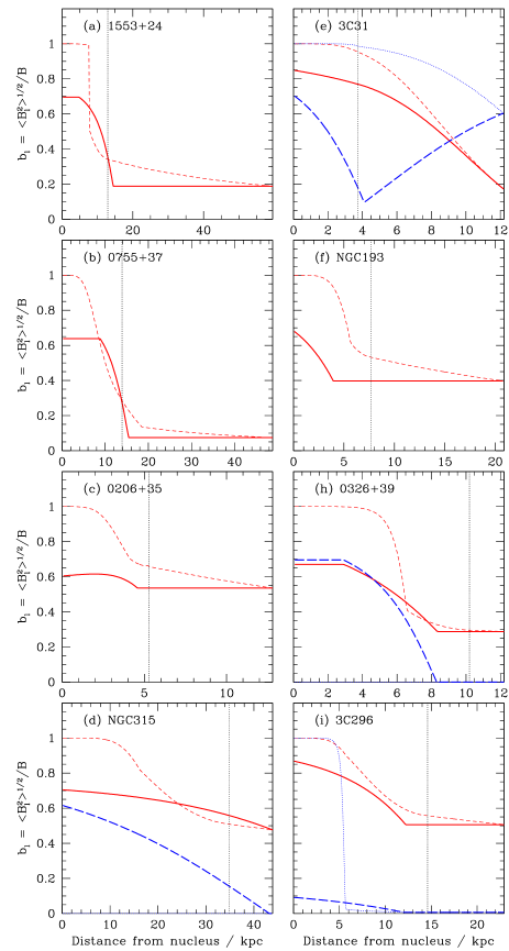
Figure 19: Comparison of fitted profiles of fractional longitudinal field, $b_{l}=\langle B_{\rm l}^{2}\rangle^{1/2}/B$, with the predictions of the simple flux-freezing model described in the text for on-axis and edge streamlines. Red, full, wide: fitted, on-axis; red, short-dashed, narrow: adiabatic on-axis; blue, long-dashed, wide: fitted, edge; blue, dotted,narrow: adiabatic, edge. If the minimal models do not include transverse variations of field component ratio, then only one pair of profiles is plotted. The vertical dotted lines indicate the recollimation distance, $r_{0}$. Field parameters for the minimal models given in Table 10 were used for all sources except 3C 31.

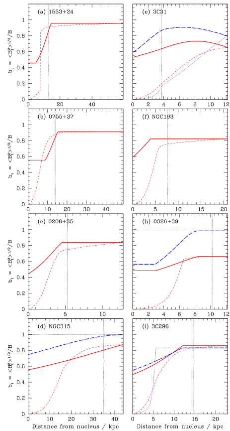
Figure 20: As Fig. 19, but for the fractional toroidal field, $b_{t}=\langle B_{\rm t}^{2}\rangle^{1/2}/B$.

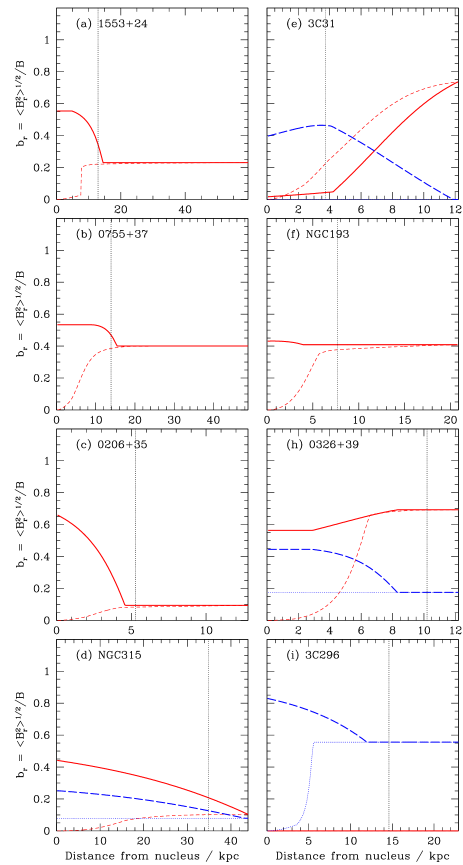
Figure 21: As Fig. 19, but for the fractional radial field, $b_{r}=\langle B_{\rm r}^{2}\rangle^{1/2}/B$.

Close to the AGN, the field component ratios predicted by flux-freezing vary much more rapidly with distance than our model fits. In other words, the transition between longitudinal and transverse field does not happen as abruptly as expected for jets which are both expanding rapidly and decelerating. For the normalization we have chosen, the flux-freezing approximation predicts that the field becomes almost entirely longitudinal close to the AGN (Fig. 19) and, conversely, that the toroidal and radial components essentially vanish (Figs 20 and 21). The only exceptions occur where the longitudinal component is close to zero at the edge of the model grid (the edge streamlines for NGC 315, 0326+39 and 3C 296). The simple reason for the discrepancy is that the ratio of longitudinal to toroidal or radial field is $\propto\Gamma\beta x^{-1}$ (equations 31 – 32). The jets expand rapidly with distance from the AGN in the geometrically flaring region and also decelerate: both effects cause $\Gamma\beta x^{-1}$ to decrease with distance (by a factor of $\approx$1300 over the model region for 3C 31, for example).

At larger distances, particularly in the outer region, the model and flux-freezing relations both tend to become flat. The fitted velocities for the minimal models are constant and the asymptotic expansion rates in the outer regions are small, so equations (31) – (32) also imply slow changes in the component ratios. To a reasonable approximation, the variation of field component ratios after the end of rapid deceleration and recollimation is consistent with flux-freezing (the one conspicuous exception, 3C 31, is the only source that continues to decelerate significantly on scales $>r_{v0}$).

It is not surprising that the approximation of flux-freezing in a quasi-one-dimensional flow fails for the high-emissivity and rapid-deceleration regions, since this is where we infer shocks (Section 8.5), strongly evolving velocity shear and turbulence. We attempted to model the evolution of the field in 3C 31 self-consistently assuming flux-freezing in a laminar velocity field with a transverse gradient (Laing & Bridle, 2004), but failed to get even approximate agreement except in the outer region. One fundamental problem is that the ratio of radial to toroidal field strength should not change with distance even in the presence of shear in a simple axisymmetric velocity field. In 3C 31 and some other sources, this is not consistent with the model fits. Another issue is that the shear vanishes on-axis in an axisymmetric velocity field of the type we consider, so it is not possible to slow the decline in longitudinal field there. A likely explanation is that random (turbulent) motions which we cannot model significantly affect the field component ratios and maintain these ratios closer to equipartition between longitudinal and transverse components than is expected from flux-freezing.

Finally, we note that the almost pure toroidal nature of the off-axis magnetic field at large distances from the AGN (Fig. 10) could have implications for jet collimation. If this field is vector-ordered and sufficiently strong, then it could at least help to confine the on-axis flow, which usually has higher emissivity (Fig. 8) and therefore by implication higher particle pressure. Vector-ordering of the toroidal field component is consistent with, but not required by our modelling.

8.4 Adiabatic models

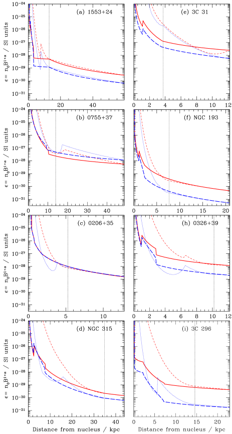
Figure 22: Comparison of fitted emissivity function profiles with the predictions of adiabatic models for the emission on-axis and at the jet edges. Red full: fitted, on-axis; red short dashed: adiabatic on-axis; blue long dashed: fitted, edge; blue dotted: adiabatic, edge. The vertical dotted lines indicate the recollimation distance, $r_{0}$.

With the assumption that the energies of the radiating particles are altered only by adiabatic losses (i.e. particle acceleration and radiative loss processes can be ignored), the emissivity function $\epsilon$ can be written in terms of the magnetic field $B$, as

$$\epsilon\propto(x^{2}\beta\Gamma)^{-(1+2\alpha/3)}B^{1+\alpha}$$ (33)

(Baum et al., 1997; Laing & Bridle, 2004). If the magnetic field follows the quasi-one-dimensional flux-freezing relations of Section 8.3, then $B$ can be expressed in terms of the field components $\langle\bar{B_{l}}^{2}\rangle^{1/2}$, $\langle\bar{B_{t}}^{2}\rangle^{1/2}$ and $\langle\bar{B_{r}}^{2}\rangle^{1/2}$, the radius $\bar{x}$, velocity $\bar{\beta}$ and Lorentz factor $\bar{\Gamma}$ at some fiducial location using equation (8) of Laing & Bridle (2004):

$$B = \left[\langle\bar{B_{l}}^{2}\rangle\left(\frac{\bar{x}}{x}\right)^{4}+(\langle\bar{B_{t}}^{2}\rangle+\langle\bar{B_{r}}^{2}\rangle)\left(\frac{\bar{\Gamma}\bar{\beta}\bar{x}}{\Gamma\beta x}\right)^{2}\right]^{1/2}$$ (34)

We can therefore predict the emissivity function using our fitted jet widths and velocities together with the modelled field component ratios at the fiducial location.

We find that the slopes of the emissivity function variations fitted by our jet models asymptotically approach those of equation (34) far from the AGN, in the region where the jets have decelerated and recollimated. In Fig. 22, we compare the emissivity function variations for our models with the predictions of equation (34) for on-axis and edge streamlines. The magnitudes of the adiabatic and model-fitted emissivities have been normalized to each other at the outer edge of the model grid for each source (again leading to the exclusion of M 84 and 3C 270). In most cases, the two emissivity-function curves agree reasonably well after the jets have both decelerated and recollimated. 3C 31 is again the exception (Fig. 22e); as for the field evolution, we suspect that this is related to continuing deceleration. In every case the adiabatic approximation predicts a much faster variation of emissivity function with distance from the AGN than is actually observed within the flaring region. In other words, the observed jets all fade much more slowly with increasing jet width in their flaring regions than would be predicted from adiabatic losses alone, but their brightness decrease becomes asymptotically adiabatic after they have recollimated. It is therefore unwise to attempt to determine the variation of jet velocity with distance assuming adiabatic brightness evolution in the flaring region, but such estimates may be valid after recollimation.

The implication of our result is that there is little ongoing particle acceleration or radiative energy loss for particles emitting at GHz frequencies in the outer regions (radiative losses are not expected to be significant since there is no evidence for spectral steepening with distance from the AGN; Laing & Bridle 2013).

In contrast, we would not expect the adiabatic relations to be followed in the flaring regions, since these parts of the jets are known to emit synchrotron radiation at all frequencies up to soft X-rays. This requires ongoing particle acceleration, as we now discuss.

8.5 Particle acceleration and radio spectra

Higher-frequency (mid- and near-IR, optical and especially X-ray) emission has now been detected from many FR I main jet bases (and one counter-jet) For the present sample, X-ray emission has been imaged with Chandra in 0206+35, 0755+37, NGC 315, 3C 31, NGC 193, M 84, 3C 296 and 3C 270 (Worrall, Birkinshaw & Hardcastle, 2001, 2003, 2007, 2010; Hardcastle et al., 2002, 2005; Harris et al., 2002; Kharb et al., 2012). Optical and/or mid-infrared detections have also been made for 1553+24, 0755+37, 3C 31 and 3C 296 (Croston et al., 2003; Hardcastle et al., 2005; Lanz et al., 2011; Parma et al., 2003). The high-frequency emission is thought to be synchrotron radiation from a higher-energy extension of the relativistic electron population responsible for the radio emission. High-frequency emission is typically detected out to the end of the high-emissivity region in the approaching jets. In two well-observed cases (NGC 315 and 3C 270), it extends as far as the end of deceleration, albeit at a lower level compared with the radio emission (Laing & Bridle, 2013, their table 3). The synchrotron lifetimes for X-ray emitting electrons are tens to hundreds of years – considerably smaller than the light-travel times across the jets. This makes a cast-iron case for ongoing particle acceleration in the regions we model.

We investigated the radio spectra of these jets over the frequency range 1.4 – 4.9 or 8.4 GHz (Laing & Bridle, 2013), with the following conclusions.

1. The spectra always flatten slightly with increasing distance from the nucleus between the brightness flaring point and the end of rapid deceleration.

2. The mean spectral indices are $\langle\alpha\rangle=0.66\pm 0.01$ over the high-emissivity region and $\langle\alpha\rangle=0.59\pm 0.01$ both immediately after deceleration and in the outer (recollimation) region. The corresponding energy indices are $q=2.32$ and 2.18, respectively (equation 1).

3. One source, NGC 315, also shows transverse spectral gradients in the sense that $\alpha$ is higher on-axis (Laing et al., 2006a).

4. The steeper spectra close to the jet flaring points are associated with typical bulk flow speeds $\beta\ga 0.5$.

This radio spectral analysis is consistent with our results from adiabatic models (Section 8.4 and Laing & Bridle 2004). Particle acceleration with $q=2.32$ over the energy range corresponding to GHz radio emission (electron Lorentz factors $\gamma\sim 2000-30000$, assuming equipartition magnetic fields) is required in the high-emissivity region. The process must be capable of accelerating electrons to $\gamma\sim 10^{7}-10^{8}$ for bulk flow speeds $\beta\ga 0.5$ (or ${\mathcal{M}}\ga 1.5-2$, as we conjecture in Section 8.2). In the deceleration region, there is a gradual transition to a characteristic energy index $q=2.18$. High-energy radiation is still produced, but is less prominent relative to the radio emission. The range of observed spectral indices and the inferred dependence on velocity could result from first-order Fermi acceleration by mildly relativistic shocks, in the limit that the scattering mean free path is close to the electron gyro-radius (Summerlin & Baring, 2012). If the bulk flow is at most mildly supersonic (Section 8.2), this mechanism may not be efficient enough, particularly in the slower, flatter-spectrum regions. A second mechanism would then be required, perhaps associated with increased velocity shear, as suggested by the transverse spectral gradients in NGC 315. After deceleration and recollimation, there is relatively little ongoing particle acceleration.

8.6 Brightness flaring and the high-emissivity region

What might cause the jet brightening that marks the onset of the extended flaring region? We do not yet have an unambiguous explanation, but can add some new constraints, as follows.

1. The outer isophotes of the jets expand at a continually increasing rate both upstream and immediately downstream of the brightness flaring points (Fig. 17).

2. The resolved radio structures in the jet bases downstream from the brightness flaring points, e.g. the quasi-helical chain of bright knots in the jet of NGC 315 (Fig. 17d) and the knots in the high-emissivity regions of the jets of 3C 31, 3C 296 and 3C 270 (Figs 17e, i and j) are complex, non-axisymmetric and concentrated towards the jet axes (perhaps located at the spine/shear-layer boundary). We find no convincing evidence for brightness enhancements that cross the entire width of the jets in their high-emissivity regions, although such structures could be present close to the flaring points themselves, where the jets are too narrow for us to resolve transversely.

3. The flow immediately downstream of the flaring point must be at least transonic: $\beta\approx 0.8$, so ${\mathcal{M}}\ga 2$, the lower limit corresponding to a jet composition dominated by ultrarelativistic particles and field (Section 8.2).

4. The brightness flaring points are located in steeply falling external pressure gradients. All of the sources with published high-resolution X-ray images show dense, kpc-scale coronae of hot gas. Fig. 23 shows the absolute and normalized pressure profiles derived from isothermal beta-model fits to Chandra observations for 0755+37, 0206+35, NGC 315, 3C 31, 3C 296 and 3C 270 (Worrall et al., 2001, 2003; Hardcastle et al., 2002, 2005; Croston et al., 2008). For a pressure profile

   $$p(r)=p(0)(1+r^{2}/r_{\rm c}^{2})^{-3\beta_{\rm atm}/2}$$ (35)

   the steepest gradient is at $r=r_{\rm c}(1+3\beta_{\rm atm})^{-1/2}$, which is in the range 0.2 – 1 kpc for the sources in Fig. 23 (core radii between 0.35 and 1.8 kpc). The corresponding flaring point distances are 0.8 – 2.6 kpc. In 0755+37, 0206+35, 3C 31 and 3C 270, the brightness flaring points are located close to the steepest pressure gradients; in NGC 315 and 3C 296, they are significantly farther out (Fig. 23).

Figure 23: Pressure profiles for the dense coronae of hot gas surrounding the jet bases in 0755+37, 0206+35, NGC 315, 3C 31, 3C 296 and 3C 270. These were derived from isothermal beta-model fits to Chandra observations (Worrall et al., 2001, 2003; Hardcastle et al., 2002, 2005; Croston et al., 2008). (a) absolute pressures, $p(r)$; (b) relative pressures $p(r)/p(0)$. $+$ symbols mark the brightness flaring points.

Three mechanisms have been suggested for the sudden brightening of FR I jets, as follows.

1. The jet is overpressured within the corona and expands rapidly until its pressure falls below that of the ambient medium, at which point a stationary recollimation shock forms (Sanders, 1983). The recollimation shock marks the flaring point and the high-emissivity region contains a series of shocks formed as the jet oscillates around pressure equilibrium. Shocks naturally lead to brightness enhancements not only from compression, but also as a result of first-order Fermi acceleration.

2. Alternatively, if the jet is initially in pressure equilibrium with the corona and the external pressure drops sufficiently steeply with distance, a standing shock (or series of shocks) can again be formed (Bicknell, 1984). Daly & Marscher (1988) analysed the case of a relativistic jet which encounters an instantaneous drop in external pressure and showed that jet-crossing shocks form when the pressure drops by more than a factor of $\approx$2.

3. Jets are likely to be unstable to the growth of Kelvin-Helmholtz instabilities (Perucho, 2012; Salvesen et al., 2013, and references therein). The pressure maxima associated with these instabilities will cause brightness enhancements, as would any particle acceleration processes associated with growth of instabilities and transition to turbulence, or small-scale shocks. The flaring point might then be the location where the growth becomes non-linear.

Case (i) was considered by Perucho & Martí (2007, simulation 1), who studied the evolution of a light, overpressured, relativistic jet propagating in the external density and pressure distribution estimated for 3C 31 (Hardcastle et al., 2002) and demonstrated the formation of strong recollimation shocks. One argument against this idea is that we see no evidence for recollimation in the outer isophotes at the brightness flaring point (in contrast to the situation at the end of the flaring region). This is not conclusive, since entrainment and mixing with the external medium will cause the jet to expand again, but we have shown that evolution of the transverse velocity profile appears to begin significantly downstream of the flaring point and we might expect the spreading rate to decrease before mixing becomes important. Finally, there is no explanation for the origin of the initial overpressure, which is imposed as an initial condition.

The alternative that the jet is in pressure equilibrium with the corona until $r\approx r_{\rm c}$, where it becomes overpressured [case(ii)], is more plausible for two reasons. First, pressure decreases are inferred from X-ray observations at approximately the correct locations (Fig. 23). Second, the outer envelope of the jet is expected to expand (on average) as it adjusts to pressure balance, as observed. The pressure decrease may be too slow for strong shocks to develop, however, so it is not clear how large a brightness enhancement would be observed.

The absence of obvious jet-crossing shocks is a potential difficulty for cases (i) and (ii).

The drop in external pressure may still be the trigger for flaring in brightness even if strong shocks are not formed. In a simulation of an initially pressure-matched jet with initial velocity $\beta=0.5$, again in the external density and pressure gradients inferred for 3C 31, Perucho & Martí (2007, simulation 4) confirmed that the cross-section of the jet oscillated smoothly and that strong shocks were not formed. In this simulation, however, the coupling to Kelvin-Helmholtz instabilities was enhanced [case (iii)]. The simulated jet disrupted shortly after the growth of instabilities, whereas the jets analysed here flare without disruption, maintaining fairly smooth outer isophotes (Fig. 17). Thus if Kelvin-Helmholtz instabilities are important at the brightness flaring points of the jets in our sample, then they are unlikely to be dominated by low-order modes.

The idea that brightness flaring is triggered by rapid expansion in a steep external pressure gradient therefore seems plausible, but the precise mechanism remains obscure.

8.7 Velocities upstream of the brightness flaring point

Figure 24: Observed values of the jet/counter-jet sidedness ratio, $I_{\rm j}/I_{\rm cj}$ determined between 2 $\times$ FWHM and $0.6r_{e1}$ (in projection) from the core for NGC 315, 3C 31, NGC 193, 0326+39, 3C 296 and 3C 270, plotted against inclination, $\theta$ from our model fits. The ratios for velocities of $\beta=0.375$ (full), $\beta=0.7$ (dotted) and $\beta=0.94$ (dashed) predicted using equation (10) are plotted for comparison.

We cannot address the question of the flow velocity upstream of the flaring point satisfactorily using our models because the jets are faint and poorly resolved transverse to their axes in these regions (Section 3.5.5). We were, however, able to measure the jet and counter-jet flux densities from where they are first separable from the core (2 $\times$ FWHM) to $0.6r_{e1}$ in projection from the AGN for six sources (we chose the outer limit to avoid any emission directly associated with the flaring points at $r=r_{e1}$). The observed sidedness ratios (plotted against $\theta$ in Fig. 24) do not show a consistent trend. We can estimate the velocity roughly using equation (10). For three sources (3C 31, NGC 193 and 3C 296), the ratios suggest a low value of $\beta\approx 0.4$; NGC 315 and 0326+39 require $\beta\approx 0.7$ ($<\beta_{1}$) and $\beta\approx 0.95$ ($>\beta_{1}$), respectively, and 3C 270 has too high a ratio to be consistent with any velocity.

The measurement of counter-jet flux densities close to the core is difficult and spatial averages are poorly defined for irregular brightness distributions. Nevertheless, the slow speeds inferred in three cases suggest two possible scenarios, which we cannot presently distinguish. The first is that the outflows as a whole are accelerating with increasing distance from the AGN upstream of the brightness flaring point, as might be the case for overpressured jets propagating in steeply-decreasing pressure profiles (e.g. simulation 1 of Perucho & Martí 2007). The alternative is that the emission from the upstream region comes mainly from a slow-moving surface layer, and that faster on-axis flow in the jet spine becomes visible only after sudden deceleration at the brightness flaring point, as previously suggested for 3C 31 by Laing & Bridle (2002a). The emission from the surface layer would have to dominate at least for $\theta\ga 50^{\circ}$. We might then expect to see emission from the spine components in the approaching jets if they are orientated closer to the line of sight, but projection would inevitably mean that they would be poorly resolved, as is indeed the case for our sources with $\theta<50^{\circ}$. An argument against this alternative is that we see little evidence for a slow boundary layer immediately downstream of the brightness flaring point, where the transverse velocity profiles are close to flat.

Independent evidence of slower speeds on parsec scales comes from proper-motion measurements. The best-studied case is M 87, which we discuss below (Section 8.8). Proper motions have been determined for the approaching jets in two of our modelled sources: NGC 315 (Cotton et al., 1999; Lister et al., 2013) and 3C 270 (Piner, Jones & Wehrle, 2001). For NGC 315, the apparent speeds measured by Cotton et al. (1999) are $\beta_{\rm app}=0.81$ at an angular separation of 4 mas from the core and $\beta_{\rm app}=1.79$ at 10 mas. For $\theta=49\aas@@fstack{\circ}8$, the corresponding pattern speeds are $\beta_{\rm pattern}=0.63$ at a deprojected distance of 1.5 pc and $\beta_{\rm pattern}=0.93$ at 4.4 pc. Lister et al. (2013) find much slower speeds: $\beta_{\rm app}=0.03-0.05$ from 2.5 to 6.4 pc and $\beta_{\rm app}<0.005$ from 0.4 to 1.7 pc ($\beta_{\rm pattern}=0.04-0.06$ and $\beta_{\rm pattern}<0.007$); these are much slower than the flow speeds inferred from the sidedness ratio (Cotton et al., 1999). We estimate a flow speed of $\beta=0.85$ on kpc scales. In 3C 270, using the distance in Table 1, the apparent speed is $\beta_{\rm app}=0.40$ at 7 mas (Piner et al., 2001), implying a pattern speed of $\beta=0.37$ at a deprojected distance of 1.1 pc for $\theta=75\aas@@fstack{\circ}9$, whereas we find a flow speed of $\beta=0.92$ on kpc scales. In both cases, the pattern speed measured close to the AGN can be significantly slower than the flow speed we estimate on larger scales. Again, it is not clear whether the inferred speeds are consistent with an accelerating bulk flow with $\beta_{\rm pattern}=\beta_{\rm flow}$: the discrepant speed estimates for NGC 315 on pc scales suggest a more complex situation. Moving features in the jet (e.g. shocks) may have $\beta_{\rm pattern}\la\beta_{\rm flow}$ or could be preferentially located in a slower surface layer, as suggested above.

8.8 Comparison with other well-resolved sources

As described in Section 2.1, the objects selected for this study are the best-resolved and brightest of the nearby FR I radio galaxies whose AGNs successfully formed large-scale radio structures with bright, wide jets and counter-jets. The jet bases of two other nearby radio galaxies that do not have these defining characteristics have also been studied in exquisite detail, and it is interesting to examine how their properties relate to those we find for our sample.

The jet and counter-jet bases in Centaurus A (Morganti, 2010, and references therein), the closest radio galaxy to the Milky Way, have been studied with high linear resolution. Proper motions of $\beta_{\rm app}=0.3-0.8$ have been measured within its main jet (Hardcastle et al., 2003; Goodger et al., 2010), providing direct evidence for outflow at near-relativistic velocities. Two identifications have been proposed for the brightness flaring point: the A1/AX1 knot complex $\approx$0.2 kpc from the AGN (Hardcastle et al., 2003) and the region at $\approx$3.5 kpc where the jet enters the inner lobe (Hardcastle, Kraft & Worrall, 2006). While its inner jet structure may be analogous to the flaring regions and fainter upstream precursors of the jet bases studied here, Cen A is likely to be an example of an outflow that has restarted in an environment disturbed by a merger of an active galaxy with a gas-rich system. It may not therefore be a good case to compare in detail with the straight, relatively undisturbed FR I jets studied here, even though it offers a close-up view of entrainment and jet-gas interactions. The faint, patchy nature of its detected counter-jet precludes modelling by our methods but if Cen A indeed contains a symmetrical decelerating outflow then the overall faintness of its counter-jet features may require flow velocities in its flaring region to exceed the pattern speeds measured by Goodger et al. (2010) and thus to be in the regime deduced here for other sources.

Studies of the spectrum of the main jet in Cen A between radio and X-ray wavelengths have provided independent evidence for multiple particle-acceleration mechanisms (Hardcastle et al., 2006, 2007; Worrall et al., 2008; Goodger et al., 2010). The X-ray emission out to 1.1 kpc in projection from the AGN is dominated by knots and is consistent with particle acceleration by small-scale shocks; acceleration between 1.1 and 4.5 kpc appears to require a distributed mechanism and the spectral evolution at larger distances is consistent with passive advection of particles. This picture is similar to the one we propose in Section 8.5 and we tentatively associate the two acceleration mechanisms with the characteristic radio spectral indices of 0.66 (shocks) and 0.59 (distributed), respectively. We cannot resolve structures on the scale of the knots in the Cen A jet in our sources, and it could be that the large-scale spectral gradients we observe result from gradual changes in the proportions of the emission from these two mechanisms.

The jet in M 87 has also been studied in detail at many wavelengths, providing clear evidence for relativistic flow. Although the measured proper motions are subrelativistic on pc scales (Reid et al., 1989; Kellermann et al., 2004; Kovalev et al., 2007), much larger speeds are found on scales $\ga$60 pc in projection with a maximum value of $\beta_{\rm app}\approx 6$ and a tendency to decrease with distance from the AGN from 100 pc outwards (Biretta, Zhou & Owen, 1995, 1999; Cheung, Harris & Stawarz, 2007; Meyer et al., 2013). Whether the changes in speed reflect true bulk acceleration and deceleration or merely changes in pattern speed in an underlying fast flow remains controversial (e.g. Kovalev et al. 2007; Nakamura & Asada 2013): a subrelativistic speed on pc scales would be inconsistent with the observed sidedness ratio. Hardee & Eilek (2011) argue from a conservation-law analysis that there is bulk deceleration from $\Gamma\approx 4.4-7.5$ at a projected distance of 80 pc to $\Gamma\approx 1.8-2.7$ ($\beta\approx 0.83-0.93$) at 1 kpc (the spectacular ‘brightening point’ at Knot ‘A’). Although the latter velocity is similar to those we infer just downstream of the brightness flaring points for the sources in our sample, there are no collimated counter-jet features in M 87 at distances from the AGN corresponding to the well-studied bright jet (even well beyond the distance of knot A) and little evidence for the geometrical flaring we observe. This lack of counter-jet emission and the small opening angle of its jet suggest that the structures in the M 87 jet are not those of a flaring region of the type described here but may instead be an example of a faster, well-collimated ‘strong-flavour’ jet seen at a small angle to our line of sight. If so, then M 87 may more closely resemble a ‘wide-angle-tail’ source seen at a small inclination angle, in which the jets disrupt rather than flaring, decelerating and recollimating smoothly.

9 Summary

We have fit intrinsically symmetrical, axisymmetric relativistic flow models to deep, high-resolution $I$, $Q$ and $U$ images of jets in ten FR I radio galaxies, using the same parametrization in all cases. Our conclusions are given below and key points are sketched in Fig. 25.

9.1 Direct inferences from the data

1. The transverse-resolved sections of the jets start with geometrically flaring regions in which the spreading rates first increase rapidly and then decrease. The jets eventually recollimate to form conical outer regions.

2. The jet brightness distributions all show sudden brightness flaring following an initial dim, well-collimated region (Fig. 3). The brightness flaring point is not associated with a clear discontinuity in the spreading rate of the outer isophotes, but is within the regime of geometrical flaring in all sources (Fig. 17).

3. Immediately downstream of the brightness flaring points and within the region of geometrical flaring, we often see bright, non-axisymmetric, knotty substructures (e.g., NGC315, 3C 31, 3C 296 and 3C 270 in Figs. 3 and 17). These define the high-emissivity region.

4. The progression of collimation and brightness changes exhibited by the brighter jet is always followed on the same physical scales by the counter-jet in the same source, while the jet/counter-jet intensity ratio generally decreases with increasing distance from the AGN (Fig. 3).

5. Near the brightness flaring point, transverse intensity profiles in the main jets tend to be centrally peaked whereas those in the counter-jets tend to be flat-topped or centrally darkened (Fig. 3).

6. The jet/counter-jet asymmetries in linear polarization are well correlated with those in total intensity and follow a common pattern in all 10 sources: there is a progression along the jet axis from apparent magnetic field parallel to the axis to field perpendicular to the axis in the main jet, whereas the apparent field in the counter-jet is always perpendicular unless the jets are very symmetrical (Fig. 5).

7. The jets and counter-jets show systematic spectral variations in the flaring regions: there are small decreases in the radio spectral index with increasing distance from values near 0.66 in the high-emissivity regions to 0.59 after recollimation. The scale of this spectral variation appears to be tied to the recollimation distance.

9.2 Inferences from model fits

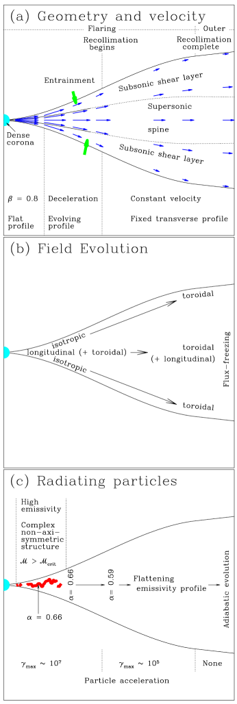
Figure 25: Sketches showing the principal deductions from our model fits. (a) Geometry, velocity field and inferred boundary-layer entrainment. The blue arrows represent the velocity field. The supersonic spine always extends into the deceleration region (where it is represented by full lines) but continues throughout the modelled region only in some cases (dotted lines). (b) Evolution of field-ordering parameters. (c) Location of the high-emissivity and adiabatic regions; spectral variations. The red pattern schematically represents bright knots in the high-emissivity region.

1. Despite the wide range of linear scales, the geometrically flaring regions (after correcting for projection using the modelled inclination and scaling by the recollimation distance, $r_{0}$) have remarkably similar shapes (Fig. 6b). The mean half-width/length ratio is 0.29 with a small dispersion.

2. Where it first becomes measurable near the AGN by our method, the outflow velocity has a mean value of $\langle\beta\rangle=0.81$ with an rms dispersion of 0.08 (Fig. 7k).

3. At this point, the transverse velocity profiles are consistent with constant values in nine of the 10 jets (Fig. 7m).

4. Farther downstream, all 10 jets decelerate with increasing distance from the AGN, although their deceleration rates vary widely (Fig. 7). Rapid deceleration occurs across the entire widths of the jets.

5. After the end of rapid deceleration, the jet velocities on a given streamline are consistent with constant values except in 3C 31, which decelerates less rapidly.

6. In six cases, there is good evidence that a transverse velocity gradient develops during deceleration: the outflow at the jet edges is slower than on-axis (Fig. 7n). Similar gradients could be present in any of the other jets.

7. In the four sources where jet speeds remain high after deceleration, the transverse velocity profiles are well determined. Their fractional edge velocities range from $\approx$0 to $\approx$0.5.

8. Jet magnetic fields are primarily longitudinal and toroidal, but not vector-ordered helices (see Section 3.1 – helical fields would lead to unobserved asymmetries in the transverse total intensity and polarization profiles). The toroidal component dominates at large distances from the AGN (Figs 9 – 11). The mean values of the rms fractional components (longitudinal:toroidal:radial) evolve:

   1. on-axis from 0.78:0.55:0.29 close to the AGN to 0.55:0.80:0.23 after recollimation and

   2. close to the edge of the jet from 0.62:0.61:0.50 (nearly isotropic) to 0.05:0.97:0.23 (almost purely toroidal).

9. Although the evolution from longitudinal to transverse field is expected in an expanding flow, the quasi-one-dimensional flux-freezing approximation predicts a much more rapid transition from longitudinal to transverse field than we infer (Figs 19 – 21). The slow evolution of field structure after recollimation is close to that expected from flux-freezing, however.

10. Downstream of the brightness flaring point, the emissivity function $\epsilon=n_{0}B^{1+\alpha}$ declines with distance from the AGN. The slope of this decline tends to flatten with increasing distance (Figs 8k and l).

11. In the flaring region, and especially in the high-emissivity region, the slope of the emissivity function is flatter than that expected if the particle energies are affected only by adiabatic losses and the field is frozen into the flow (‘adiabatic approximation’). After the jets have recollimated and decelerated, the two slopes are similar (Fig. 22). The implication is that particle acceleration is required throughout the flaring region, but not after recollimation.

12. The characteristic spectral index $\alpha\approx 0.66$ observed in the high-emissivity region is associated with jet speeds $\beta\ga 0.5$ (Section 8.5; Laing & Bridle 2013).

13. The flaring regions are homologous structures, in the sense that the fiducial distances for velocity, emissivity function and magnetic field evolution scale linearly with the recollimation distance, $r_{0}$ (Table 4; Fig. 18). The brightness flaring point marks a discontinuity in some combination of speed and rest-frame emissivity function, located at $\approx$0.1$r_{0}$. The high-emissivity region runs from $\approx$0.1$r_{0}$ to $\approx$0.3$r_{0}$. Rapid deceleration starts midway along the high-emissivity region (at $\approx$0.2$r_{0}$; Fig. 17) and lasts until $\approx$0.6$r_{0}$. Magnetic evolution begins near the AGN and essentially stops just after the end of the flaring region, at $\approx$1.1$r_{0}$ (where flux-freezing becomes a reasonable approximation).

14. The end of rapid deceleration coincides accurately with the start of recollimation (i.e. where the spreading rate begins to decrease with distance; Fig. 18g).

15. The inclination angles of the jets inferred from our modelling correlate well with other indicators of the jet orientation: fractional core flux density (Section 6.4) and Faraday rotation rms ratio (Section 6.6).

16. We find a remarkably good correlation between the core luminosity (corrected for Doppler boosting) and the extended luminosity for our sample, despite the large difference in physical scale between the emitting regions (Fig. 14c).

17. We have analysed the effects of departures from intrinsic symmetry in emissivity function, using the statistics of reversals in jet sidedness to estimate the magnitude of the effect. We find that the effects on our derived physical parameters are comparable with other uncertainties for $\theta\la 75^{\circ}$, but dominate at larger inclinations.

9.3 Further inferences about jet physics

We conjecture the following about the internal physics of the jets from the systematics given above.

1. The jet has a mildly supersonic spine, of which the high-emissivity region forms the base. The composition is dominated by ultrarelativistic particles and magnetic field at the brightness flaring point, giving an internal Mach number ${\mathcal{M}}\approx 2$ for $\beta\approx 0.8$ and the sound speed decreases as matter is entrained. The high-emissivity region is the volume over which ${\mathcal{M}}\ga{\mathcal{M}}_{\rm crit}=1.5-1.8$.

2. A subsonic shear layer forms at the edge of the jet at or slightly downstream of the brightness flaring point. As it grows, a measurable transverse velocity gradient develops across the jet and the spine also decelerates.

3. Jet evolution is remarkably similar in twin-jet sources with and without lobes. Jets in both classes of source propagate in direct contact with the external medium within the dense, hot, kpc-scale coronae that always surround their AGN and the majority of entrainment occurs in these regions. As the external environment becomes more tenuous, owing to the jet entering a lobe or to a rapid decrease in the density of the external galactic atmosphere, the entrainment rate drops. The flow velocity then usually reaches an asymptotic value, preserving its previously acquired transverse gradient, and the jet starts to recollimate, eventually spreading at a low and constant rate. An exception is 3C 31, whose continuing deceleration on large scales can be accounted for by the availability of group-scale gas for entrainment.

4. Depending on the amount of entrainment, the shear layer may expand to fill the entire jet or the supersonic spine may persist after deceleration and recollimation.

5. Steeper radio spectra ($\alpha=0.66$) and acceleration of particles up to Lorentz factors of $10^{7}-10^{8}$ occur in the supersonic flow before the jets decelerate significantly. A possible mechanism is Fermi acceleration by mildly relativistic shocks (Summerlin & Baring, 2012).

6. Flatter spectra ($\alpha=0.59$) and lower maximum Lorentz factors ($10^{5}-10^{6}$) are associated with the flow after deceleration. These could be produced by Fermi acceleration with a lower shock velocity or by a second acceleration mechanism, perhaps associated with velocity shear.

7. The trigger for jet deceleration remains unclear, but we note that the brightness flaring points are always located on the edges of the dense coronae, in steeply-falling external pressure gradients. It is plausible that the jets become overpressured and that this results in the formation of internal shocks and/or in the non-linear growth of Kelvin-Helmholtz modes. Although the high-emissivity regions of several of the jets contain complex, non-axisymmetric brightness features (Fig. 17), these are not obviously consistent with either possibility, and observations at higher angular resolution may be needed to distinguish between different explanations for the flaring.

Appendix A Coordinate definitions and fitting functions

In this section, we tabulate the fitting functions for geometry, velocity, emissivity function and magnetic-field ordering. Expressions for outflow and backflow components are given in Tables 5 and 6, respectively.

Table 5: Coordinate definitions and functional forms for geometry, velocity, emissivity function and magnetic-field ordering. (1) physical quantity; (2) symbol, as used in the text; (3) functional form; (4) range of distance coordinate, $r$, over which the expression is applicable.

Description	Quantity	Functional form	Distance range
Distance coordinate	$r$	$zr_{0}/[(r_{0}+A)\cos\xi-A]$	$r\leq r_{0}$
		$(z+A)/\cos\xi-A$	$r\geq r_{0}$
		$A=x_{0}/\sin\xi_{0}-r_{0}$
Streamline index	$s$	by continuity	$r\leq r_{0}$
		$\xi/\xi_{0}$	$r\geq r_{0}$
Radius	$x(z,s)$	$a_{2}(s)z^{2}+a_{3}(s)z^{3}$	$r\leq r_{0}$
		$(z-r_{0}+x_{0}/\sin\xi_{0})\tan\xi_{0}s$	$r\geq r_{0}$
Velocity	$\beta(r,s)$	$\beta_{1}\exp(s^{2}\ln v_{1})$	$r\leq r_{v_{1}}$
		$\beta_{1}\exp(s^{2}\ln v_{1})\left(\frac{r_{v0}-r}{r_{v0}-r_{v1}}\right)+\beta_{0}\exp(s^{2}\ln v_{0})\left(\frac{r-r_{v1}}{r_{v0}-r_{v1}}\right)$	$r_{v1}\leq r\leq r_{v0}$
		$\beta_{0}\exp(s^{2}\ln v_{0})\left(\frac{r_{\rm grid}-r}{r_{\rm grid}-r_{v0}}\right)+\beta_{f}\exp(s^{2}\ln v_{f})\left(\frac{r-r_{v0}}{r_{\rm grid}-r_{v0}}\right)$	$r_{v0}\leq r\leq r_{\rm grid}$
Emissivity function	$\epsilon(r,s)$	$g_{1}\left(\frac{r}{r_{e1}}\right)^{-E_{\rm in}}\exp(s^{2}\ln e_{1})$	$r\leq r_{e1}$
		$~{}~{}~{}\left(\frac{r}{r_{e1}}\right)^{-E_{\rm mid}}\exp\left[\ln\left(s^{2}\frac{e_{1}(r_{e0}-r)+e_{0}(r-r_{e1})}{r_{e0}-r_{e1}}\right)\right]$	$r_{e1}<r\leq r_{e0}$
		$g_{0}\left(\frac{r}{r_{e0}}\right)^{-E_{\rm out}}\left(\frac{r_{e0}}{r_{e1}}\right)^{-E_{\rm mid}}\exp\left[s^{2}\ln\left(\frac{e_{0}(r_{\rm grid}-r)+e_{f}(r-r_{e0})}{r_{\rm grid}-r_{e0}}\right)\right]$	$r_{e0}<r\leq r_{0}$
		$g_{0}\left(\frac{r}{r_{0}}\right)^{-E_{\rm far}}\left(\frac{r_{0}}{r_{e0}}\right)^{-E_{\rm out}}\left(\frac{r_{e0}}{r_{e1}}\right)^{-E_{\rm mid}}\exp\left[s^{2}\ln\left(\frac{e_{0}(r_{\rm grid}-r)+e_{f}(r-r_{e0})}{r_{\rm grid}-r_{e0}}\right)\right]$	$r_{0}\leq r\leq r_{\rm grid}$
$\langle B_{r}^{2}/B_{t}^{2}\rangle^{1/2}$	$j(r,s)$	$j^{\rm cen}+(j^{\rm edge}-j^{\rm cen})s^{w_{j}}$
		$j^{\rm edge}=j_{1}^{\rm edge}$	$r\leq r_{B1}$
		$j^{\rm edge}=\frac{j_{1}^{\rm edge}(r_{B0}-r)+j_{0}^{\rm edge}(r-r_{B1})}{r_{B0}-r_{B1}}$; $j^{\rm cen}=\frac{j_{1}^{\rm cen}(r_{B0}-r)+j_{0}^{\rm cen}(r-r_{B1})}{r_{B0}-r_{B1}}$	$r_{B1}\leq r\leq r_{B0}$
		$j^{\rm edge}=\frac{j_{0}^{\rm edge}(r_{\rm grid}-r)+j_{f}^{\rm edge}(r-r_{B0})}{r_{\rm grid}-r_{B0}}$; $j^{\rm cen}=\frac{j_{0}^{\rm cen}(r_{\rm grid}-r)+j_{f}^{\rm cen}(r-r_{B0})}{r_{\rm grid}-r_{B0}}$	$r_{B0}\leq r\leq r_{\rm grid}$
$\langle B_{l}^{2}/B_{t}^{2}\rangle^{1/2}$	$k(r,s)$	$k^{\rm cen}+(k^{\rm edge}-k^{\rm cen})s^{w_{k}}$
		$k^{\rm edge}=k_{1}^{\rm edge}$	$r\leq r_{B1}$
		$k^{\rm edge}=\frac{k_{1}^{\rm edge}(r_{B0}-r)+k_{0}^{\rm edge}(r-r_{B1})}{r_{B0}-r_{B1}}$; $k^{\rm cen}=\frac{k_{1}^{\rm cen}(r_{B0}-r)+k_{0}^{\rm cen}(r-r_{B1})}{r_{B0}-r_{B1}}$	$r_{B1}\leq r\leq r_{B0}$
		$k^{\rm edge}=\frac{k_{0}^{\rm edge}(r_{\rm grid}-r)+k_{f}^{\rm edge}(r-r_{B0})}{r_{\rm grid}-r_{B0}}$; $k^{\rm cen}=\frac{k_{0}^{\rm cen}(r_{\rm grid}-r)+k_{f}^{\rm cen}(r-r_{B0})}{r_{\rm grid}-r_{B0}}$	$r_{B0}\leq r\leq r_{\rm grid}$

Table 6: Functional forms for geometry, velocity, emissivity function and magnetic-field ordering in backflow components. These are exactly as in Table 4 of Laing & Bridle (2012), and are given here for completeness. (1) physical quantity; (2) symbol, as used in Table 11; (3) functional form; (4) range of distance coordinate, $r$, over which the expression is applicable.

Description	Quantity	Functional form	Distance range
Backflow streamline index	$t$	by continuity	$r\leq r_{0}$
		$(\xi-\xi_{0})/(\xi_{\rm b}-\xi_{0})$	$r\geq r_{0}$
Backflow radius	$x(z,s)$	$a_{2}(t)z^{2}+a_{3}(t)z^{3}$	$r\leq r_{0}$
		$(z-r_{0}+x_{0}/\sin\xi_{\rm b})\tan\xi_{\rm b}s$	$r\geq r_{0}$
Backflow velocity	$\beta(t)$	$\beta_{\rm b,in}+t(\beta_{\rm b,out}-\beta_{\rm b,in})$
Backflow emissivity function	$\epsilon(r,t)$	0	$r<r_{b}$
		$n_{\rm b}(r/r_{0})^{-E_{\rm b}}\exp(\ln e_{\rm b}t^{2})$	$r\geq r_{b}$
Backflow $\langle B_{r}^{2}/B_{t}^{2}\rangle^{1/2}$	$j$	$j_{\rm b}$
Backflow $\langle B_{l}^{2}/B_{t}^{2}\rangle^{1/2}$	$k$	$k_{\rm b}$

Appendix B $\chi^{2}$ values for the fits

In Table 7, we list the values of $\chi^{2}$ for the best-fitting full and minimal models. These are summed over the Stokes parameters $I$, $Q$ and $U$. The number of points is $\Sigma n_{\rm pixel}n_{\rm Stokes}$, where $n_{\rm pixel}$ is the number of independent sampling points and $n_{\rm Stokes}$ is the number of Stokes parameters evaluated at that pixel. The areas over which $I$, $Q$ and $U$ were evaluated were always the same. Identical points were normally used for all Stokes parameters (in which case the sum is just $3\Sigma n_{\rm pixel}$), but we occasionally used the higher-resolution image over a larger fraction of the area for $I$.

Fig. 26 shows plots of $\chi^{2}$ against inclination, $\theta$, illustrating the lower bound described in Section 3.6.

Table 7: $\chi^{2}$ values for the fits. (1) Source name; (2) number of resolutions; (3) $\chi^{2}$ for the full models, summed over $I$, $Q$ and $U$; (4) number of independent points. (5) and (6) as (3) and (4), but for the minimal models.

Source	nres	Full		Minimal
		$\chi^{2}$	N	$\chi^{2}$	N
1553+24	2	4690.5	4566	4821.5	4566
NGC 315	2	5715.1	7368	5783.7	7368
3C 31	2	5244.8	3753
NGC 193	2	7047.0	5718	7236.9	5706
M 84	1	7857.1	5106
0326+39	2	4185.4	3594	4328.3	3594
0755+37	2	7962.6	5816	8022.4	5816
0206+35	1	7634.4	6708	8012.5	6696
3C 296	2	7671.5	8025	7677.5	8025
3C 270	1	8090.8	6384	8151.6	6384

Figure 26: Plots of $\chi^{2}$ against angle to the line of sight, $\theta$, for the full models. Crosses and filled squares are for optimizations with fixed and variable $\theta$, respectively. The numbers of independent points are given in Table 7. The horizontal, dashed lines represent the $\chi^{2}$ thresholds used to define error ranges (Section 3.7).

Appendix C Notes on models for individual sources

1553+24

Our earlier model for this source gave a very small angle to the line of sight, $\theta\approx 8^{\circ}$ (Canvin & Laing, 2004). A more systematic search of parameter space using optimizations with fixed values of $\theta$ (Section 3.6) showed that this represented a local minimum in $\chi^{2}$. The main reason for the difficulty in finding the global minimum is low signal-to-noise: 1553+24 is the weakest source in our sample. The true minimum lies in a unusually broad range, $10^{\circ}\la\theta\la 40^{\circ}$ (Fig. 26a), but the derived velocity, emissivity function and field parameters are close to those given in Table 8 for any inclination in this range. The new best-fitting inclination, $\theta=25^{\circ}$ is more reasonable than the 8° found by Canvin & Laing (2004): 1553+24 has a bright core and a one-sided optical jet, consistent with a fairly low inclination, but does not show any of the nuclear properties of a BL Lac object, as would be expected if $\theta\la 10^{\circ}$, and the deprojected linear size of the extended structure is now less extreme. As noted by Canvin & Laing (2004), the increase of jet/counter-jet sidedness ratio at large distances from the AGN is consistent with small intrinsic differences and may not require bulk acceleration. The fitting functions used by Canvin & Laing (2004), in particular for emissivity function, differ significantly from those in this paper, making comparison difficult. The main substantive difference is that we find a higher initial velocity, consistent with the increased inclination.

0755+37

This is one of the two sources for which we include a mildly relativistic backflow in our models. The minimal model for this source is exactly as given by Laing & Bridle (2012), who describe the backflow component in detail, and the full model is very similar. The values of $r_{v0}$ and $r_{e0}$ in 0755+37 are anomalous (Fig. 18b, d and g), perhaps because the counter-jet emission is dominated by the backflow component at large distances from the AGN, making it difficult to determine fiducial distances for the outflow.

0206+35

This is the second source for which we include a backflow component in the model. The minimal model is as in Laing & Bridle (2012); the full model differs only slightly.

NGC 315

Our earlier model of NGC 315 fit only the straight inner $\pm$70 arcsec of the jets (Canvin et al., 2005). In order to constrain the flow parameters after recollimation, we have extended the model region to $\pm$100 arcsec, after correcting for the slight bends observed in both jets. The minimal model we tabulate for NGC 315 is described in detail by Laing & Bridle (in preparation); the full model is very similar. The technique of optimizing at fixed $\theta$ showed that the inclination found by Canvin et al. (2005) corresponded to a local minimum in $\chi^{2}$ and that the true value is close to 50°. As a consequence, our fitted velocities are slightly faster than those given by Canvin et al. (2005). The fit places the outer magnetic fiducial distance close to the edge of the grid. We therefore fixed $r_{B0}=r_{\rm grid}$ to avoid convergence problems and no error is quoted for it.

3C 31

The fitting functions used for 3C 31 by Laing & Bridle (2002a) differ significantly from those in this paper. Laing & Bridle (2002a) assumed a conical inner region close to the nucleus of 3C 31, but this is not required to fit the data and we found no evidence for such a structure in better-resolved cases. Two forms of transverse structure were investigated by Laing & Bridle (2002a): spine/shear-layer (in which parameter values in the two components are independent) and Gaussian (as in this paper). The former gave only a slightly better fit, at the expense of a large number of additional parameters, so we do not consider it here. Despite the different fitting functions, our new model is very similar to that described by Laing & Bridle (2002a); for example, the smooth analytical form of the velocity profile assumed by Laing & Bridle (2002a) is close to the piecewise linear function of Fig. 2(a). $E_{\rm out}$ is not defined for 3C 31 because the high-emissivity region ends very close to recollimation.

NGC 193

The minimal model for this sources is described by Laing & Bridle (in preparation); the full model is very similar.

M 84

This small, intrinsically weak source is clearly interacting strongly with its environment, and the assumptions of intrinsic symmetry and axisymmetry fail closer to the nucleus than in any other case we have modelled. It is important to our study primarily because of its very low power. The model is exactly as given by Laing & Bridle (in preparation). Although the total length of the model grid was $\pm 20$ arcsec, we only show a field of $\pm 12.5$ arcsec, since the fits are poor at larger distances from the AGN, where there is evidence for asymmetrical interactions with the local environment (Laing & Bridle, in preparation). The projections on the sky of the recollimation distance, $r_{0}$ and the fiducial distances for velocity and emissivity function, $r_{v1}$ and $r_{e1}$, are larger than 12.5 arcsec, so the parameters defined at $r_{\rm grid}$ (subscript $f$) do not influence the fits in the region we show. They are therefore omitted from Table 8.

0326+39

The new model is very similar to that derived by Canvin & Laing (2004).

3C 296

Compared with the observed images fit by Laing et al. (2006b), those used here have been corrected for surrounding lobe emission and a slight bend in the outer counter-jet. The new model includes a radial field component, and therefore provides a slightly better description of the polarization structure in the outer main jet. Otherwise, the changes from Laing et al. (2006b) are small. The prominent knot at the base of the counter-jet is not well fitted by any outflow model, as it is wider than the main jet at the same distance from the AGN.

3C 270

The model fit for 3C 270 is described in detail by Laing et al. (in preparation). It is a difficult source to model for several reasons. Firstly, systematic asymmetries in intensity and polarization are relatively small (the jet inclination is the largest in our sample) so intrinsic side-to-side differences have a significant effect even close to the AGN. The derived inclination of $\theta=76\degr$ is at the practical upper limit for our technique (Section 7.2). Secondly, fits for fiducial distances are slightly different in the two jets. Finally, there are large areas of oblique apparent magnetic field which are inconsistent with any axisymmetric model (Fig. 27j), so the polarization fits are poor and the local degree of polarization is underestimated in the outer jets. The fitted parameters describing the flow at projected distances $\ga$15 arcsec (where the fit is poor) should be treated with caution.

Appendix D Polarization vector plots

In Fig. 27, we show comparisons between the observed and model linear polarizations, in the form of vector images. The format is similar to that of Figs 3 – 5, with panels (a) – (j) showing model and observed images arranged in order of increasing fitted angle to the line of sight, but the individual panels are kept separate in the interests of legibility. The final panel (k) shows the observations only for 3C 449.

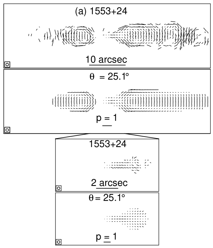
Figure 27: (a) Comparison between observed and model polarization vector images for 1553+24. The lengths of the vectors are proportional to the degree of polarization, $p=P/I$, and their directions are those of the apparent magnetic field. The plots are arranged in pairs, as in Figs 3 – 5. The upper and lower panels of each pair show the observed image (labelled with the source name) and the model image (with the fitted value of $\theta$), respectively. The core is at the centre of each plot, and the brighter (approaching) jet is to the right. The angular scale is indicated by a labelled bar on the upper panel, the vector scale by a bar on the lower panel and the FWHM of the beam by a circle at the bottom of each plot. The comparison at high resolution is shown below that at low resolution with the relative areas indicated. The observed values of $P$ have been corrected for Ricean bias (Wardle & Kronberg, 1974). The observed and model images are both blanked wherever $I<5\sigma_{I}$ ($\sigma_{I}$ is the off-source noise level). Field sizes and resolutions are given in Table 2.

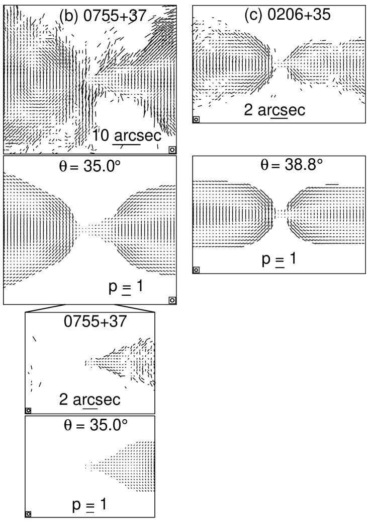
Figure 28: continued

(b) 0755+37; (c) 0206+35

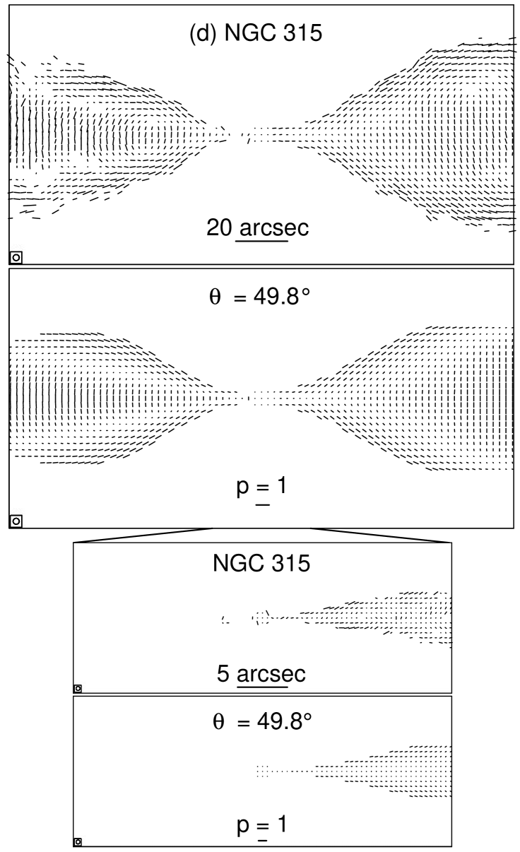
Figure 29: continued

(d) NGC 315.

Figure 30: continued

(e) 3C 31.

Figure 31: continued

(f) NGC 193.

Figure 32: continued

(g) M 84; (h) 0326+39.

Figure 33: continued

(i) 3C 296.

Figure 34: continued

(j) 3C 270.

Figure 35: continued

(k) 3C 449. Only observed images are shown for this source.

Appendix E Tabulated values of fiducial parameters

Tables 8 and 10 list the values of the fitted parameters and their errors for our full and minimal models, respectively. In Table 11, we give the parameters of the backflow components for 0206+25 and 0755+37 as defined by Laing & Bridle (2012). These are not discussed in this paper, but are tabulated here for completeness.

Table 8: Fitted parameters for the full model outflows. The variables are defined in Section 3.5 and Table 5, except for the inclination range, $\Delta\theta$ (Section 3.7). Col. 1 gives the variable name; the remaining 10 columns refer to the modelled sources, in order of increasing angle to the line of sight. Angles are in degrees and fiducial distances are in kpc. Values in brackets were used to compute the brightness distributions in Figs 3 – 5 and 27, but have almost no effect on them and are effectively unconstrained. The bracketed fractional edge velocities multiply central velocities which are close to zero and the bracketed values of $w_{j}$ and $w_{k}$ occur in cases where the centre and edge field ratios are nearly the same. $-$ means that the parameter is not defined (see Appendix C).

Var-	Source
iable	1553+24	0755+37	0206+35	NGC 315	3C 31	NGC 193	M 84	0326+39	3C 296	3C 270
Distances fixed in projection
$r_{\rm min}$	$0.48$	$0.73$	$0.39$	$0.07$	$0.12$	$0.16$	$0.06$	$0.12$	$0.14$	$0.18$
$r_{\rm grid}$	$59.5$	$48.6$	$13.1$	$43.9$	$12.2$	$21.9$	$2.12$	$12.2$	$22.9$	$6.26$
Geometry
$\theta$	$25.1_{-0.9}^{+0.8}$	$35.0_{-1.1}^{+0.8}$	$38.8_{-1.7}^{+1.0}$	$49.8_{-0.2}^{+0.5}$	$52.5_{-0.9}^{+0.5}$	$55.2_{-1.2}^{+3.5}$	$58.3_{-2.1}^{+2.8}$	$60.6_{-2.8}^{+3.0}$	$65.0_{-0.8}^{+1.4}$	$75.9_{-2.5}^{+2.6}$
$\Delta\theta$	$10-39$	$32.5-38.5$	$33-41$	$47-54$	$40-60$	$45-62.5$	$55-62$	$55-70$	$62.5-68$	$71-79$
$\xi_{0}$	$3.4_{-0.8}^{+0.4}$	$7.4_{-0.1}^{+0.2}$	$3.8_{-0.3}^{+0.9}$	$7.6_{-1.4}^{+3.5}$	$13.7_{-0.5}^{+0.3}$	$5.8_{-1.1}^{+0.7}$	$12.6_{-2.1}^{+3.4}$	$2.1_{-1.0}^{+4.1}$	$5.9_{-1.2}^{+1.1}$	$9.9_{-2.2}^{+1.9}$
$r_{0}$	$12.9_{-0.2}^{+0.6}$	$13.9_{-0.4}^{+0.2}$	$5.41_{-0.07}^{+0.21}$	$34.9_{-0.4}^{+1.7}$	$3.72_{-0.06}^{+0.07}$	$8.1_{-0.2}^{+0.2}$	$1.80_{-0.02}^{+0.05}$	$10.3_{-0.2}^{+0.6}$	$14.6_{-0.2}^{+0.3}$	$5.19_{-0.09}^{+0.10}$
$x_{0}$	$3.08_{-0.36}^{+0.06}$	$3.88_{-0.05}^{+0.09}$	$1.32_{-0.05}^{+0.02}$	$11.1_{-0.7}^{+0.2}$	$0.83_{-0.03}^{+0.02}$	$3.06_{-0.18}^{+0.07}$	$0.58_{-0.03}^{+0.01}$	$2.43_{-0.19}^{+0.04}$	$6.02_{-0.21}^{+0.06}$	$1.25_{-0.06}^{+0.04}$
Velocity
$r_{v1}$	$7.4_{-1.3}^{+0.9}$	$3.6_{-1.5}^{+1.6}$	$1.8_{-0.3}^{+0.3}$	$6.6_{-1.1}^{+0.8}$	$2.3_{-0.4}^{+0.6}$	$0.0_{-0.0}^{+0.7}$	$0.28_{-0.08}^{+0.10}$	$1.7_{-1.1}^{+0.8}$	$3.6_{-0.5}^{+0.6}$	$1.99_{-0.16}^{+0.18}$
$r_{v0}$	$8.3_{-1.2}^{+0.8}$	$18.6_{-1.4}^{+2.5}$	$4.6_{-0.3}^{+0.2}$	$16.2_{-1.0}^{+0.7}$	$3.9_{-0.4}^{+0.5}$	$5.5_{-0.5}^{+0.5}$	$1.41_{-0.08}^{+0.06}$	$7.0_{-0.6}^{+0.8}$	$5.8_{-0.3}^{+0.4}$	$4.4_{-0.3}^{+0.3}$
$\beta_{1}$	$0.95_{-0.09}^{+0.01}$	$0.88_{-0.04}^{+0.05}$	$0.83_{-0.05}^{+0.09}$	$0.85_{-0.03}^{+0.02}$	$0.71_{-0.04}^{+0.05}$	$0.72_{-0.07}^{+0.08}$	$0.76_{-0.06}^{+0.06}$	$0.82_{-0.11}^{+0.09}$	$0.70_{-0.07}^{+0.06}$	$0.92_{-0.02}^{+0.03}$
$\beta_{0}$	$0.19_{-0.03}^{+0.04}$	$0.25_{-0.10}^{+0.07}$	$0.72_{-0.10}^{+0.09}$	$0.55_{-0.05}^{+0.02}$	$0.57_{-0.04}^{+0.04}$	$0.18_{-0.02}^{+0.03}$	$0.00_{-0.00}^{+0.03}$	$0.02_{-0.02}^{+0.05}$	$0.58_{-0.05}^{+0.06}$	$0.00^{+0.06}$
$\beta_{f}$	$0.28_{-0.08}^{+0.10}$	$0.26_{-0.09}^{+0.15}$	$0.62_{-0.14}^{+0.17}$	$0.62_{-0.07}^{+0.07}$	$0.13_{-0.02}^{+0.04}$	$0.12_{-0.09}^{+0.10}$	$-$	$0.20_{-0.11}^{+0.08}$	$0.58_{-0.05}^{+0.07}$	$0.12_{-0.12}^{+0.20}$
$v_{1}$	$1.00_{-0.15}^{+0.00}$	$1.00_{-0.07}^{+0.00}$	$0.93_{-0.10}^{+0.07}$	$1.00_{-0.07}^{+0.00}$	$1.00_{-0.18}^{+0.00}$	$0.97_{-0.24}^{+0.03}$	$0.99_{-0.18}^{+0.01}$	$0.58_{-0.22}^{+0.24}$	$0.96_{-0.25}^{+0.04}$	$0.81_{-0.04}^{+0.05}$
$v_{0}$	$0.40_{-0.21}^{+0.36}$	$0.25_{-0.19}^{+0.21}$	$0.02_{-0.01}^{+0.01}$	$0.36_{-0.08}^{+0.04}$	$0.47_{-0.08}^{+0.12}$	$0.91_{-0.40}^{+0.09}$	$(0.07)$	$(0.64)$	$0.01_{-0.01}^{+0.00}$	$(0.31)$
$v_{f}$	$0.43_{-0.29}^{+0.57}$	$0.27_{-0.17}^{+0.48}$	$0.11_{-0.07}^{+0.09}$	$0.36_{-0.12}^{+0.11}$	$1.00_{-0.32}^{+0.00}$	$(0.86)$	$-$	$(0.70)$	$0.01_{-0.01}^{+0.00}$	$(0.43)$
Emissivity Function
$r_{e1}$	$1.00_{-0.10}^{+0.08}$	$1.54_{-0.03}^{+0.03}$	$0.81_{-0.02}^{+0.03}$	$2.6_{-0.5}^{+0.3}$	$1.17_{-0.13}^{+0.16}$	$1.18_{-0.08}^{+0.10}$	$0.30_{-0.24}^{+0.10}$	$1.03_{-0.19}^{+0.15}$	$2.3_{-0.5}^{+0.5}$	$1.4_{-0.4}^{+0.4}$
$r_{e0}$	$3.36_{-0.10}^{+0.08}$	$10.1_{-0.2}^{+0.2}$	$2.10_{-0.07}^{+0.08}$	$7.77_{-0.25}^{+0.46}$	$3.70_{-0.10}^{+0.12}$	$2.53_{-0.23}^{+0.14}$	$0.72_{-0.04}^{+0.03}$	$2.88_{-0.09}^{+0.10}$	$7.30_{-0.16}^{+0.13}$	$3.87_{-0.11}^{+0.10}$
$E_{\rm in}$	$4.2_{-0.8}^{+0.6}$	$2.4_{-1.1}^{+0.9}$	$(2.8)$	$4.15_{-0.15}^{+0.09}$	$(2.6)$	$(2.5)$	$(0.7)$	$4.5_{-0.3}^{+0.2}$	$(0.4)$	$(2.3)$
$E_{\rm mid}$	$4.37_{-0.14}^{+0.16}$	$3.76_{-0.04}^{+0.04}$	$2.64_{-0.09}^{+0.08}$	$3.07_{-0.16}^{+0.13}$	$3.23_{-0.09}^{+0.11}$	$3.60_{-0.30}^{+0.22}$	$0.60_{-0.55}^{+0.35}$	$2.44_{-0.31}^{+0.28}$	$3.10_{-0.15}^{+0.14}$	$3.28_{-0.19}^{+0.19}$
$E_{\rm out}$	$0.12_{-0.09}^{+0.08}$	$1.15_{-0.26}^{+0.25}$	$1.94_{-0.10}^{+0.08}$	$3.03_{-0.07}^{+0.08}$	$-$	$2.12_{-0.08}^{+0.07}$	$2.61_{-0.14}^{+0.10}$	$1.29_{-0.12}^{+0.07}$	$0.89_{-0.09}^{+0.06}$	$0.2_{-0.3}^{+0.3}$
$E_{\rm far}$	$1.99_{-0.10}^{+0.10}$	$1.17_{-0.10}^{+0.09}$	$2.23_{-0.16}^{+0.21}$	$2.08_{-0.92}^{+1.10}$	$1.39_{-0.06}^{+0.05}$	$2.16_{-0.11}^{+0.11}$	$-$	$1.82_{-1.22}^{+1.29}$	$0.89_{-0.11}^{+0.15}$	$2.1_{-0.5}^{+1.0}$
$e_{1}$	$1.6_{-0.4}^{+0.7}$	$1.1_{-0.3}^{+0.2}$	$1.2_{-0.4}^{+1.1}$	$1.4_{-0.4}^{+0.4}$	$0.26_{-0.07}^{+0.08}$	$0.6_{-0.2}^{+0.2}$	$0.4_{-0.1}^{+0.2}$	$0.8_{-0.3}^{+0.5}$	$0.14_{-0.04}^{+0.04}$	$0.72_{-0.17}^{+0.18}$
$e_{0}$	$0.21_{-0.07}^{+0.11}$	$2.30_{-0.50}^{+0.37}$	$1.19_{-0.22}^{+0.21}$	$0.44_{-0.07}^{+0.11}$	$0.35_{-0.06}^{+0.06}$	$0.11_{-0.03}^{+0.03}$	$0.00_{-0.00}^{+0.00}$	$0.19_{-0.09}^{+0.06}$	$0.04_{-0.01}^{+0.01}$	$0.12_{-0.03}^{+0.09}$
$e_{f}$	$0.33_{-0.13}^{+0.19}$	$2.30_{-0.43}^{+0.70}$	$0.97_{-0.28}^{+0.43}$	$0.44_{-0.10}^{+0.14}$	$0.25_{-0.05}^{+0.03}$	$0.13_{-0.04}^{+0.04}$	$-$	$0.17_{-0.05}^{+0.07}$	$0.04_{-0.01}^{+0.01}$	$0.14_{-0.05}^{+0.04}$
$g_{1}$	$0.17_{-0.07}^{+0.08}$	$1.73_{-0.49}^{+0.43}$	$1.61_{-1.41}^{+1.42}$	$0.13_{-0.03}^{+0.03}$	$0.31_{-0.18}^{+0.22}$	$0.29_{-0.18}^{+0.16}$	$(0.9)$	$0.15_{-0.07}^{+0.06}$	$1.2_{-0.6}^{+0.5}$	$1.2_{-0.3}^{+0.4}$
$g_{0}$	$0.16_{-0.02}^{+0.02}$	$0.52_{-0.03}^{+0.05}$	$1.14_{-0.10}^{+0.08}$	$0.49_{-0.05}^{+0.05}$	$1.03_{-0.05}^{+0.05}$	$1.17_{-0.11}^{+0.19}$	$0.81_{-0.07}^{+0.15}$	$0.35_{-0.04}^{+0.06}$	$0.87_{-0.05}^{+0.05}$	$1.12_{-0.10}^{+0.12}$

Table 9: continued

Var-	Source
iable	1553+24	0755+37	0206+35	NGC 315	3C 31	NGC 193	M 84	0326+39	3C 296	3C 270
Field component ratios
$r_{B1}$	$2.2_{-2.2}^{+4.5}$	$8.8_{-1.9}^{+2.7}$	$0.0_{-0.0}^{+1.3}$	$0.0_{-0.0}^{+2.2}$	$0.0_{-0.0}^{+0.5}$	$0.0_{-0.0}^{+0.8}$	$0.0_{-0.0}^{+0.2}$	$3.2_{-1.0}^{+1.1}$	$0.0_{-0.0}^{+1.1}$	$1.2_{-0.5}^{+0.5}$
$r_{B0}$	$14.2_{-1.9}^{+2.1}$	$15.0_{-2.7}^{+2.4}$	$4.7_{-0.5}^{+0.6}$	$43.9$	$4.2_{-0.5}^{+0.4}$	$4.3_{-0.5}^{+0.5}$	$1.38_{-0.06}^{+0.09}$	$8.0_{-0.9}^{+0.9}$	$12.2_{-0.6}^{+0.9}$	$4.9_{-0.2}^{+0.3}$
$j_{1}^{\rm cen}$	$0.6_{-0.5}^{+0.3}$	$1.0_{-0.4}^{+0.4}$	$1.5_{-1.3}^{+0.9}$	$0.8_{-0.3}^{+0.3}$	$0.0_{-0.0}^{+1.4}$	$0.9_{-0.8}^{+0.8}$	$1.3_{-0.5}^{+0.4}$	$1.3_{-0.5}^{+0.5}$	$0.0_{-0.0}^{+0.4}$	$0.6_{-0.6}^{+0.5}$
$j_{1}^{\rm edge}$	$2.1_{-0.3}^{+0.3}$	$1.0_{-0.2}^{+0.2}$	$1.5_{-0.4}^{+0.4}$	$0.3_{-0.1}^{+0.2}$	$0.7_{-0.4}^{+0.3}$	$0.9_{-0.5}^{+0.4}$	$0.7_{-0.5}^{+0.7}$	$0.8_{-0.4}^{+0.4}$	$1.5_{-1.5}^{+2.3}$	$0.6_{-0.3}^{+0.4}$
$j_{0}^{\rm cen}$	$0.4_{-0.4}^{+0.3}$	$0.6_{-0.6}^{+0.7}$	$0.2_{-0.2}^{+0.4}$	$0.1_{-0.1}^{+0.5}$	$0.1_{-0.1}^{+0.7}$	$0.7_{-0.2}^{+0.2}$	$0.4_{-0.1}^{+0.2}$	$1.1_{-0.4}^{+0.3}$	$0.0_{-0.0}^{+0.2}$	$1.0_{-0.2}^{+0.2}$
$j_{0}^{\rm edge}$	$0.0_{-0.0}^{+0.3}$	$0.3_{-0.3}^{+0.2}$	$0.1_{-0.1}^{+0.1}$	$0.0_{-0.0}^{+0.2}$	$0.5_{-0.1}^{+0.1}$	$0.3_{-0.2}^{+0.1}$	$0.3_{-0.2}^{+0.2}$	$0.2_{-0.2}^{+0.3}$	$0.7_{-0.7}^{+1.0}$	$1.1_{-0.3}^{+0.2}$
$j_{f}^{\rm cen}$	$0.9_{-0.9}^{+1.2}$	$0.5_{-0.5}^{+1.4}$	$0.2_{-0.2}^{+2.2}$	$-$	$1.1_{-1.1}^{+0.7}$	$1.0_{-0.6}^{+0.7}$	$-$	$1.0_{-0.5}^{+0.6}$	$0.0_{-0.0}^{+0.3}$	$0.9_{-0.3}^{+0.5}$
$j_{f}^{\rm edge}$	$0.1_{-0.1}^{+1.1}$	$0.5_{-0.3}^{+0.4}$	$0.1_{-0.1}^{+0.8}$	$-$	$0.0_{-0.0}^{+0.1}$	$0.5_{-0.5}^{+0.4}$	$-$	$0.1_{-0.1}^{+0.5}$	$0.7_{-0.7}^{+2.5}$	$1.0_{-0.4}^{+0.4}$
$k_{1}^{\rm cen}$	$1.8_{-0.8}^{+1.1}$	$1.2_{-0.2}^{+0.2}$	$1.5_{-0.4}^{+0.5}$	$1.3_{-0.1}^{+0.1}$	$1.6_{-0.3}^{+0.2}$	$1.4_{-0.3}^{+0.2}$	$1.5_{-0.2}^{+0.3}$	$1.3_{-0.4}^{+0.7}$	$1.8_{-0.1}^{+0.1}$	$1.7_{-0.4}^{+0.4}$
$k_{1}^{\rm edge}$	$1.7_{-0.1}^{+0.2}$	$1.16_{-0.09}^{+0.08}$	$1.4_{-0.2}^{+0.2}$	$0.8_{-0.1}^{+0.1}$	$1.2_{-0.3}^{+0.2}$	$1.0_{-0.3}^{+0.3}$	$0.9_{-0.2}^{+0.2}$	$1.2_{-0.1}^{+0.2}$	$0.2_{-0.2}^{+0.1}$	$1.6_{-0.2}^{+0.3}$
$k_{0}^{\rm cen}$	$0.3_{-0.3}^{+1.2}$	$0.1_{-0.1}^{+1.3}$	$0.9_{-0.2}^{+0.1}$	$0.6_{-0.1}^{+0.1}$	$1.2_{-0.1}^{+0.0}$	$0.5_{-0.1}^{+0.1}$	$0.8_{-0.1}^{+0.1}$	$0.5_{-0.5}^{+0.6}$	$0.59_{-0.06}^{+0.04}$	$0.78_{-0.10}^{+0.13}$
$k_{0}^{\rm edge}$	$0.2_{-0.2}^{+0.3}$	$0.1_{-0.1}^{+0.6}$	$0.5_{-0.2}^{+0.1}$	$0.0_{-0.0}^{+0.1}$	$0.1_{-0.1}^{+0.1}$	$0.3_{-0.2}^{+0.1}$	$0.0_{-0.0}^{+0.1}$	$0.0_{-0.0}^{+0.2}$	$0.01_{-0.01}^{+0.05}$	$0.75_{-0.11}^{+0.12}$
$k_{f}^{\rm cen}$	$0.1_{-0.1}^{+3.6}$	$0.1_{-0.1}^{+0.7}$	$0.8_{-0.3}^{+0.2}$	$-$	$0.3_{-0.2}^{+0.1}$	$0.6_{-0.4}^{+0.2}$	$-$	$0.3_{-0.3}^{+1.0}$	$0.58_{-0.07}^{+0.08}$	$0.8_{-0.2}^{+0.2}$
$k_{f}^{\rm edge}$	$0.3_{-0.3}^{+0.7}$	$0.1_{-0.1}^{+0.3}$	$0.6_{-0.4}^{+0.2}$	$-$	$0.7_{-0.1}^{+0.2}$	$0.5_{-0.5}^{+0.4}$	$-$	$0.2_{-0.2}^{+0.3}$	$0.00_{-0.00}^{+0.10}$	$0.75_{-0.20}^{+0.18}$
$w_{j}$	$1.5_{-0.5}^{+0.8}$	$(1.1)$	$(1.0)$	$0.7_{-0.5}^{+0.9}$	$0.3_{-0.3}^{+0.3}$	$0.8_{-0.4}^{+0.7}$	$(1.2)$	$1.1_{-0.4}^{+0.6}$	$(10)$	$(1.1)$
$w_{k}$	$(0.3)$	$(0.9)$	$1.0_{-0.4}^{+0.8}$	$1.3_{-0.2}^{+0.2}$	$1.4_{-0.2}^{+0.2}$	$1.5_{-0.9}^{+1.1}$	$0.6_{-0.1}^{+0.1}$	$0.4_{-0.4}^{+0.9}$	$1.2_{-0.1}^{+0.1}$	$(0.9)$

Table 10: Fitted parameters for minimal model outflows (see the description in the caption for Table 8).

Var-	Source
iable	1553+24	0755+37	0206+35	NGC 315	NGC 193	0326+39	3C 296	3C 270
Distances fixed in projection
$r_{\rm min}$	$0.48$	$0.73$	$0.38$	$0.07$	$0.16$	$0.12$	$0.14$	$0.19$
$r_{\rm grid}$	$62.0$	$48.8$	$12.8$	$43.9$	$20.9$	$12.2$	$22.9$	$6.42$
Geometry
$\theta$	$25.0_{-1.2}^{+0.8}$	$34.8_{-0.8}^{+0.7}$	$40.0_{-0.3}^{+0.3}$	$49.8_{-0.5}^{+0.3}$	$59.7_{-2.8}^{+1.6}$	$61.1_{-1.6}^{+3.2}$	$65.0_{-1.1}^{+1.3}$	$76.1_{-2.4}^{+2.9}$
$\Delta\theta$	$10-40$	$32.5-37.5$	$34-43$	$48-54.5$	$51-65$	$55-70$	$63-68.5$	$70-79$
$\xi_{0}$	$3.4_{-0.8}^{+0.4}$	$7.4_{-0.1}^{+0.2}$	$3.9_{-0.2}^{+0.2}$	$7.6_{-2.0}^{+2.6}$	$6.1_{-1.0}^{+0.9}$	$2.1_{-1.3}^{+3.0}$	$5.9_{-1.2}^{+1.1}$	$9.9_{-1.4}^{+3.0}$
$r_{0}$	$12.9_{-0.2}^{+0.6}$	$13.9_{-0.3}^{+0.3}$	$5.3_{-0.1}^{+0.1}$	$34.9_{-0.4}^{+1.3}$	$7.7_{-0.2}^{+0.1}$	$10.2_{-0.1}^{+0.5}$	$14.6_{-0.2}^{+0.3}$	$5.38_{-0.07}^{+0.14}$
$x_{0}$	$3.08_{-0.41}^{+0.06}$	$3.88_{-0.06}^{+0.08}$	$1.32_{-0.04}^{+0.02}$	$11.1_{-0.6}^{+0.2}$	$3.06_{-0.09}^{+0.10}$	$2.43_{-0.19}^{+0.03}$	$6.02_{-0.20}^{+0.07}$	$1.30_{-0.09}^{+0.03}$
Velocity
$r_{v1}$	$7.6_{-1.1}^{+0.6}$	$3.6_{-1.5}^{+1.6}$	$1.8_{-0.3}^{+0.3}$	$6.6_{-1.2}^{+0.7}$	$0.0_{-0.0}^{+0.7}$	$1.8_{-0.9}^{+1.0}$	$3.6_{-0.5}^{+0.6}$	$2.1_{-0.2}^{+0.2}$
$r_{v0}$	$7.7_{-0.7}^{+1.0}$	$18.5_{-1.5}^{+2.3}$	$4.1_{-0.2}^{+0.3}$	$16.2_{-1.1}^{+0.6}$	$5.7_{-0.5}^{+0.5}$	$6.6_{-0.7}^{+0.7}$	$5.8_{-0.3}^{+0.4}$	$4.5_{-0.2}^{+0.3}$
$\beta_{1}$	$0.95_{-0.07}^{+0.01}$	$0.88_{-0.04}^{+0.05}$	$0.86_{-0.07}^{+0.08}$	$0.85_{-0.03}^{+0.01}$	$0.75_{-0.06}^{+0.08}$	$0.81_{-0.10}^{+0.10}$	$0.70_{-0.07}^{+0.05}$	$0.92_{-0.02}^{+0.03}$
$\beta_{0}$	$0.21_{-0.03}^{+0.02}$	$0.25_{-0.05}^{+0.07}$	$0.68_{-0.05}^{+0.09}$	$0.55_{-0.02}^{+0.03}$	$0.18_{-0.02}^{+0.03}$	$0.07_{-0.03}^{+0.05}$	$0.58_{-0.03}^{+0.04}$	$0.00_{-0.00}^{+0.10}$
$v_{1}$	$0.98_{-0.10}^{+0.02}$	$1.00_{-0.06}^{+0.00}$	$0.95_{-0.13}^{+0.05}$	$1.00_{-0.08}^{+0.00}$	$0.98_{-0.18}^{+0.02}$	$0.55_{-0.20}^{+0.28}$	$0.96_{-0.26}$	$0.81_{-0.04}^{+0.06}$
$v_{0}$	$0.54_{-0.21}^{+0.25}$	$0.26_{-0.11}^{+0.19}$	$0.04_{-0.01}^{+0.02}$	$0.36_{-0.04}^{+0.05}$	$0.97_{-0.35}^{+0.03}$	$(0.82)$	$0.01_{-0.01}^{+0.00}$	$(0.78)$
Emissivity Function
$r_{e1}$	$1.16_{-0.12}^{+0.11}$	$1.55_{-0.03}^{+0.04}$	$0.80_{-0.02}^{+0.02}$	$2.55_{-0.36}^{+0.35}$	$1.12_{-0.10}^{+0.08}$	$1.01_{-0.20}^{+0.13}$	$2.25_{-0.45}^{+0.58}$	$1.4_{-0.4}^{+0.5}$
$r_{e0}$	$3.34_{-0.06}^{+0.11}$	$10.2_{-0.3}^{+0.1}$	$2.04_{-0.06}^{+0.09}$	$7.77_{-0.23}^{+0.47}$	$2.46_{-0.19}^{+0.14}$	$2.85_{-0.10}^{+0.08}$	$7.30_{-0.15}^{+0.14}$	$4.00_{-0.14}^{+0.09}$
$E_{\rm in}$	$4.5_{-0.3}^{+0.3}$	$(2.4)$	$(3.1)$	$4.2_{-0.1}^{+0.1}$	$(2.7)$	$4.5_{-0.3}^{+0.2}$		$(2.4)$
$E_{\rm mid}$	$4.4_{-0.1}^{+0.2}$	$3.76_{-0.04}^{+0.02}$	$2.59_{-0.08}^{+0.09}$	$3.07_{-0.14}^{+0.15}$	$3.6_{-0.2}^{+0.3}$	$2.4_{-0.4}^{+0.2}$	$3.1_{-0.1}^{+0.2}$	$3.3_{-0.2}^{+0.2}$
$E_{\rm out}$	$0.2_{-0.1}^{+0.1}$	$1.16_{-0.09}^{+0.05}$	$2.13_{-0.06}^{+0.08}$	$3.03_{-0.04}^{+0.12}$	$2.12_{-0.05}^{+0.05}$	$1.3_{-0.1}^{+0.1}$	$0.89_{-0.05}^{+0.05}$	$0.2_{-0.5}^{+0.2}$
$E_{\rm far}$	$1.9_{-0.1}^{+0.1}$	$-$	$-$	$2.1_{-0.9}^{+1.3}$	$-$	$-$		$2.0_{-0.8}^{+0.7}$
$e_{1}$	$1.9_{-0.3}^{+0.9}$	$1.0_{-0.2}^{+0.3}$	$1.2_{-0.5}^{+0.6}$	$1.5_{-0.4}^{+0.5}$	$0.5_{-0.2}^{+0.2}$	$0.7_{-0.3}^{+0.4}$	$0.2_{-0.1}^{+0.1}$	$0.69_{-0.21}^{+0.14}$
$e_{0}$	$0.24_{-0.07}^{+0.07}$	$2.2_{-0.3}^{+0.5}$	$1.14_{-0.18}^{+0.16}$	$0.44_{-0.06}^{+0.09}$	$0.11_{-0.01}^{+0.05}$	$0.18_{-0.06}^{+0.06}$	$0.04_{-0.01}^{+0.01}$	$0.14_{-0.04}^{+0.05}$
$g_{1}$	$0.23_{-0.05}^{+0.07}$	$1.7_{-0.4}^{+0.5}$	$1.7_{-1.3}^{+0.8}$	$0.13_{-0.03}^{+0.03}$	$0.26_{-0.13}^{+0.22}$	$0.14_{-0.06}^{+0.05}$	$1.2_{-0.6}^{+0.5}$	$1.2_{-0.4}^{+0.3}$
$g_{0}$	$0.18_{-0.03}^{+0.02}$	$0.52_{-0.03}^{+0.06}$	$1.05_{-0.09}^{+0.08}$	$0.49_{-0.06}^{+0.05}$	$1.08_{-0.11}^{+0.16}$	$0.35_{-0.04}^{+0.06}$	$0.86_{-0.04}^{+0.06}$	$1.13_{-0.08}^{+0.16}$
Field component ratios
$r_{B1}$	$4.8_{-2.4}^{+4.0}$	$8.8_{-2.0}^{+2.8}$	$0.0_{-0.0}^{+1.4}$	$0.0_{-0.0}^{+2.1}$	$0.0_{-0.0}^{+0.8}$	$2.9_{-1.5}^{+0.7}$	$0.0_{-0.0}^{+1.2}$	$1.3_{-0.7}^{+0.4}$
$r_{B0}$	$14.5_{-2.4}^{+2.0}$	$15.4_{-3.2}^{+2.5}$	$4.6_{-0.5}^{+0.5}$	$43.9$	$3.9_{-0.5}^{+0.7}$	$8.3_{-0.9}^{+0.9}$	$12.2_{-0.6}^{+0.9}$	$5.1_{-0.4}^{+0.2}$
$j_{1}^{\rm cen}$	$1.21_{-0.18}^{+0.13}$	$0.96_{-0.09}^{+0.13}$	$1.50_{-0.22}^{+0.34}$	$0.8_{-0.3}^{+0.3}$	$0.7_{-0.2}^{+0.4}$	$1.2_{-0.4}^{+0.7}$	$0.0_{-0.0}^{+0.4}$	$0.62_{-0.19}^{+0.26}$
$j_{1}^{\rm edge}$	$-$	$-$	$-$	$0.3_{-0.1}^{+0.2}$	$-$	$0.8_{-0.3}^{+0.5}$	$1.5_{-1.5}^{+2.3}$	$-$
$j_{0}^{\rm cen}$	$0.24_{-0.24}^{+0.16}$	$0.44_{-0.15}^{+0.12}$	$0.11_{-0.11}^{+0.13}$	$0.1_{-0.1}^{+0.5}$	$0.50_{-0.05}^{+0.09}$	$1.1_{-0.3}^{+0.3}$	$0.0^{+0.2}$	$0.99_{-0.08}^{+0.11}$
$j_{0}^{\rm edge}$	$-$	$-$	$-$	$0.1_{-0.1}^{+0.1}$	$-$	$0.2_{-0.2}^{+0.2}$	$0.7_{-0.7}^{+0.9}$	$-$
$k_{1}^{\rm cen}$	$1.52_{-0.08}^{+0.13}$	$1.15_{-0.07}^{+0.08}$	$1.36_{-0.13}^{+0.13}$	$1.3_{-0.1}^{+0.1}$	$1.16_{-0.14}^{+0.15}$	$1.4_{-0.6}^{+0.4}$	$1.75_{-0.10}^{+0.14}$	$1.64_{-0.17}^{+0.14}$
$k_{1}^{\rm edge}$	$-$	$-$	$-$	$0.8_{-0.1}^{+0.1}$	$-$	$1.2_{-0.1}^{+0.3}$	$0.17_{-0.13}^{+0.17}$	$-$
$k_{0}^{\rm cen}$	$0.20_{-0.20}^{+0.20}$	$0.08_{-0.08}^{+0.22}$	$0.64_{-0.04}^{+0.05}$	$0.6_{-0.1}^{+0.1}$	$0.48_{-0.03}^{+0.04}$	$0.4_{-0.4}^{+0.4}$	$0.59_{-0.04}^{+0.03}$	$0.76_{-0.05}^{+0.04}$
$k_{0}^{\rm edge}$	$-$	$-$	$-$	$0.0_{-0.0}^{+0.1}$	$-$	$0.0_{-0.0}^{+0.1}$	$0.01_{-0.01}^{+0.04}$	$-$
$w_{j}$	$-$	$-$	$-$	$0.7_{-0.5}^{+1.0}$	$-$	$1.1_{-0.4}^{+0.6}$	$(9.6)$	$-$
$w_{k}$	$-$	$-$	$-$	$1.3_{-0.2}^{+0.3}$	$-$	$0.4_{-0.6}^{+0.6}$	$1.2_{-0.1}^{+0.1}$	$-$

Table 11: Fitted parameters for backflow components, as defined in Laing & Bridle (2012). (1) Variable name (Laing & Bridle, 2012, Table 6 of this paper); (2) unit; (3) values for minimal model of 0755+37; (4) values for full model of 0755+37; (5) and (6) as (3) and (4), but for 0206+35. The parameters for the minimal models are exactly as given by Laing & Bridle (2012). Those for the full models, which are very similar (columns 4 and 6) come from optimizations with the full set of outflow parameters listed in Table 8.

Variable		Source
		0755+37		0206+35
		min	full	min	full
Geometry
$\xi_{\rm back}$	deg	$15.6_{-0.1}^{+0.5}$	$15.7_{-0.1}^{+0.5}$	$10.9_{-0.5}^{+0.5}$	$10.6_{-0.8}^{+2.6}$
$r_{\rm back}$	kpc	$23.2_{-0.7}^{+0.8}$	$23.1_{-0.8}^{+0.8}$	$2.7_{-0.2}^{+0.1}$	$2.7_{-0.1}^{+0.2}$
Velocity
$\beta_{\rm back}^{\rm in}$		$0.25_{-0.07}^{+0.04}$	$0.24_{-0.06}^{+0.05}$	$0.02_{-0.02}^{+0.03}$	$0.02_{-0.02}^{+0.04}$
$\beta_{\rm back}^{\rm out}$		$0.35_{-0.05}^{+0.05}$	$0.36_{-0.05}^{+0.05}$	$0.20_{-0.07}^{+0.06}$	$0.18_{-0.07}^{+0.06}$
Emissivity Function
$n_{\rm back}$	$\times 100$	$0.094_{-0.010}^{+0.000}$	$0.094_{-0.005}^{+0.006}$	$2.3_{-0.2}^{+0.2}$	$2.3_{-0.1}^{+0.2}$
$E_{\rm back}$		$1.81_{-0.05}^{+0.07}$	$1.82_{-0.06}^{+0.06}$	$1.66_{-0.07}^{+0.06}$	$1.64_{-0.08}^{+0.04}$
$e_{\rm back}$		$0.79_{-0.14}^{+0.13}$	$0.80_{-0.11}^{+0.18}$	$0.05_{-0.01}^{+0.02}$	$0.06_{-0.02}^{+0.02}$
Field component ratios
$j_{\rm back}$		$0.38_{-0.07}^{+0.07}$	$0.38_{-0.07}^{+0.07}$	$0.24_{-0.07}^{+0.08}$	$0.23_{-0.03}^{+0.10}$
$k_{\rm back}$		$0.03_{-0.03}^{+0.15}$	$0.01_{-0.01}^{+0.17}$	$0.38_{-0.09}^{+0.08}$	$0.35_{-0.07}^{+0.12}$

References

- (1)
- Baum et al. (1997) Baum S.A., et al., 1997, ApJ, 483, 178 (erratum ApJ, 492, 854)
- Begelman et al. (1984) Begelman M.C., Blandford R.D., Rees, M.J., 1984, Rev. Mod. Phys., 56, 255
- Bicknell (1984) Bicknell G.V., 1984, ApJ, 286, 68
- Bicknell (1994) Bicknell G.V., 1994, ApJ, 422, 452
- Biretta et al. (1999) Biretta J.A., Sparks W.B., Macchetto F., 1999, ApJ, 520, 621
- Biretta et al. (1995) Biretta J.A., Zhou F., Owen F.N., 1995, ApJ, 447, 582
- Blandford & Königl (1979) Blandford, R.D., Königl, A., 1979, ApJ, 232, 34
- Boettcher et al. (2012) Boettcher M., Harris D.E., Krawczynski H., 2012, Relativistic Jets from Active Galactic Nuclei, Wiley, Berlin
- Bowman et al. (1996) Bowman M., Leahy J.P., Komissarov S.S., 1996, MNRAS, 279, 899
- Bridle (1982) Bridle A.H., 1982, in Heeschen D.S, Wade C.M., eds, Proc. IAU Symp. 92, Extragalactic Radio Sources, Kluwer, Dordrecht, p. 121
- Bridle (1984) Bridle A.H., 1984, AJ, 89, 979
- Burch (1979) Burch S.F., 1979, MNRAS, 187, 187
- Canvin & Laing (2004) Canvin J.R., Laing R.A., 2004, MNRAS, 350, 1342
- Canvin et al. (2005) Canvin J.R., Laing R.A., Bridle A.H., Cotton W.D., 2005, MNRAS, 363, 1223
- Cappellari et al. (2011) Cappellari, M., et al., 2011, MNRAS, 413, 813
- Cheung, Harris & Stawarz (2007) Cheung C.C., Harris D.E., Stawarz L., 2007, ApJ, 663, L65
- Cotton et al. (1999) Cotton W.D., Feretti L., Giovannini G., Lara L., Venturi T., 1999, ApJ, 519, 108
- Croston et al. (2003) Croston J.H., Birkinshaw M., Conway E., Davies R.L., 2003, MNRAS, 339, 82
- Croston et al. (2008) Croston J.H., Hardcastle M.J., Birkinshaw M., Worrall D.M., Laing R.A., 2008, MNRAS, 386, 1709
- Daly & Marscher (1988) Daly R.A., Marscher A.P., 1988, ApJ, 334, 539
- de Ruiter et al. (1990) De Ruiter H.R., Parma P., Fanti C., Fanti R., 1990, A&A, 227, 351
- De Young (1993) De Young D.S., 1993, ApJ, 405, 13
- De Young (2010) De Young D.S., 2010, ApJ, 710, 743
- Dimotakis (2005) Dimotakis P.E., 2005, Annu. Rev. Fluid Mech., 37, 329
- Dimotakis, Miake-Lye & Papantoniou (1983) Dimotakis P.E., Miake-Lye R.C., Papantoniou D.A., 1983, Phys. Fluids, 26, 3185
- Falco et al. (1999) Falco E.E., et al., 1999, PASP, 111, 438
- Fanaroff & Riley (1974) Fanaroff B.L., Riley J.M., 1974, MNRAS, 167, 31P
- Feretti et al. (1999) Feretti L., Perley R., Giovannini, G., Andernach H., 1999, A&A, 341, 29
- Finoguenov et al. (2008) Finoguenov A., Ruszkowski M., Jones C., Brüggen M., Vikhlinin A., Mandel, E., 2008, ApJ, 686, 911
- Garrington & Conway (1991) Garrington S.T., Conway R.G., 1991, MNRAS, 250, 198
- Giovannini et al. (2001) Giovannini G., Cotton W.D., Feretti L., Lara L., Venturi T., 2001, ApJ, 552, 508
- Giovannini et al. (1988) Giovannini G., Feretti L., Gregorini L. Parma, P., 1988, A&A, 199, 73
- Goodger et al. (2010) Goodger J.L., et al. 2010, ApJ, 708, 675
- Guidetti et al. (2010) Guidetti D., Laing R.A., Murgia M., Govoni F., Gregorini L., Parma P., 2010, A&A, 514, A50
- Guidetti et al. (2011) Guidetti D., Laing R.A., Bridle A.H., Parma P., Gregorini L., 2011, MNRAS, 413, 2525
- Guidetti et al. (2012) Guidetti D., Laing R.A., Croston J.H., Bridle A.H., Parma P., 2012, MNRAS, 423, 1335
- Hardcastle et al. (2007) Hardcastle M.J. et al, 2007, ApJ, 670, L81
- Hardcastle et al. (2006) Hardcastle M.J., Kraft R.P., Worrall D.M., 2006, MNRAS, 368, L15
- Hardcastle et al. (2002) Hardcastle M.J., Worrall D.M., Birkinshaw M., Laing, R.A., Bridle A.H., 2002, MNRAS, 334, 182
- Hardcastle et al. (2005) Hardcastle M.J., Worrall D.M., Birkinshaw M., Laing R.A., Bridle A.H., 2005, MNRAS, 358, 843
- Hardcastle et al. (2003) Hardcastle M.J., Worrall D.M., Kraft R.P., Forman W.R., Jones C., Murray S.S., 2003, ApJ, 593, 169
- Hardee & Eilek (2011) Hardee P.E., Eilek J.A., 2011, ApJ, 735, 61
- Harris et al. (2002) Harris D.E., Finoguenov A., Bridle A.H., Hardcastle M.J., Laing R.A., 2002, ApJ, 580, 110
- Huarte-Espinosa et al. (2011) Huarte-Espinosa M., Krause M., Alexander P., 2011, MNRAS, 418, 1621
- Jetha, Hardcastle & Sakelliou (2006) Jetha N.N., Hardcastle M.J., Sakelliou I. 2006, MNRAS, 368, 609
- Kellermann et al. (2004) Kellerman K.I. et al., 2004, ApJ, 609, 539
- Kharb et al. (2012) Kharb P., O’Dea C.P., Tilak A., Baum S.A., Haynes E., Noel-Storr J., Fallon C., Christiansen K., 2012, ApJ, 754, 1
- Komissarov (1994) Komissarov S.S., 1994, MNRAS, 269, 394
- Komossa & Böhringer (1999) Komossa S., Böhringer H., 1999, A&A, 344, 755
- Königl (1980) Königl A., 1980, Phys Fluids, 23, 1083
- Kovalev et al. (2007) Kovalev Y.Y., Lister M.L., Homan D.C., Kellermann K.I., 2007, ApJ, 668, L27
- Krause et al. (2012) Krause M., Alexander P., Riley J., Hopton, D. 2012, MNRAS, 427, 3196
- Laing (1981) Laing R.A., 1981, ApJ, 248, 87
- Laing (1988) Laing R.A., 1988, Nat, 331, 149
- Laing (1993) Laing R.A., 1993, in Burgarella, D., Livio, M., O’Dea, C.P., eds, Space Telescope Sci. Inst. Symp. 6: Astrophysical Jets. Cambridge University Press, Cambridge, p. 95
- Laing (2002) Laing R.A., 2002, MNRAS, 329, 417
- Laing & Bridle (2002a) Laing R.A., Bridle A.H., 2002a, MNRAS, 336, 328
- Laing & Bridle (2002b) Laing R.A., Bridle A.H., 2002b, MNRAS, 336, 1161
- Laing & Bridle (2004) Laing R.A., Bridle A.H., 2004, MNRAS, 348, 1459
- Laing & Bridle (2012) Laing R.A., Bridle A.H., 2012, MNRAS, 424, 1149
- Laing & Bridle (2013) Laing R.A., Bridle A.H., 2013, MNRAS, 432, 1114
- Laing et al. (2008a) Laing R.A., Bridle A.H., Parma P., Feretti L., Giovannini G., Murgia M., Perley R.A., 2008a, MNRAS, 386, 657
- Laing et al. (2008b) Laing R.A., Bridle A.H., Parma P., Murgia M., 2008b, MNRAS, 391, 521
- Laing et al. (2003) Laing R.A., Canvin J.R., Bridle A.H., 2003, AN, 327, 523
- Laing et al. (2006a) Laing R.A., Canvin J.R., Cotton W.D., Bridle A.H., 2006a, MNRAS, 368, 48
- Laing et al. (2006b) Laing R.A., Canvin J.R., Bridle A.H., Hardcastle M.J., 2006b, MNRAS, 372, 510
- Laing et al. (2011) Laing R.A., Guidetti D., Bridle A.H., Parma P., Bondi M., 2011, MNRAS, 417, 2789
- Laing et al. (1999) Laing R. A., Parma P., de Ruiter H. R., Fanti R., 1999, MNRAS, 306, 513
- Laing et al. (1983) Laing R.A., Riley J.M., Longair M.S., 1983, MNRAS, 204, 151
- Lanz et al. (2011) Lanz L., Bliss A., Kraft R.P., Birkinshaw M., Lal D.V., Forman W.R., Jones C., Worrall D.M., 2011, ApJ, 731, 52
- Leahy (1993) Leahy J.P., 1993, in Röser H.J., Meisenheimer K., eds, Lecture Notes in Physics, Vol. 421, Jets in Extragalactic Radio Sources, Springer-Verlag, Berlin, p. 1
- Leahy et al. (2000) Leahy J.P., Bridle A.H., Strom R.G., 2000, http://www.jb.man.ac.uk/atlas
- Lister et al. (2013) Lister M.L., et al., 2013, AJ, 146, 120
- Loken et al. (1995) Loken C.M., Roettiger K., Burns J.O., Norman, M., 1995, ApJ, 445, 80
- Mack et al. (1997) Mack K.-H., Klein U., O’Dea C.P., Willis A.G., 1997, A&AS, 123, 423
- Meyer et al. (2013) Meyer E.T., Sparks W.B., Biretta J.A., Anderson J., Sohn S.T., van der Marel R.P., Norman C., Nakamura M., 2013, ApJ, 774, L21
- Miller et al. (2002) Miller N.A., Ledlow M.J., Owen F.N., Hill J.M., 2002, AJ, 123, 3018
- Morganti (2010) Morganti R., 2010, PASA, 27, 463
- Morganti et al. (1997) Morganti R., Parma P., Capetti A., Fanti R., de Ruiter H.R., 1997, A&A, 326, 919
- Nakamura & Asada (2013) Nakamura M., Asada K., 2013, ApJ, 775, 118
- Nelder & Mead (1965) Nelder J.A., Mead R., 1965, Comput. J., 7, 308
- Ogando et al. (2008) Ogando R.L.C., Maia M.A.G., Pellegrini P.S., da Costa L.N., 2008, AJ, 135, 2424
- O’Sullivan et al. (2011) O’Sullivan E., Worrall D.M., Birkinshaw M., Trinchieri G., Wolter A., Zezas A., Giacintucci S, 2011, MNRAS, 416, 2916
- Parma et al. (1987) Parma P., Fanti C., Fanti R., Morganti R., de Ruiter H.R., 1987, A&A, 181, 244
- Parma et al. (2003) Parma P., de Ruiter H.R., Capetti A., Fanti R., Morganti R., Bondi M., Laing R.A., Canvin J.R., 2003, A&A, 397, 127
- Perucho (2012) Perucho M., 2012, Int. J. of Mod. Phys. Conf. Ser., 8, 241
- Phinney (1983) Phinney E.S., 1983, PhD thesis, Univ. Cambridge
- Perucho & Martí (2007) Perucho M., Martí J. M., 2007, MNRAS, 382, 526
- Piner et al. (2001) Piner B.G., Jones D.L., Wehrle A.E., 2001, AJ, 122, 2954
- Press et al. (2007) Press W.H., Teukolsky S.A., Vetterling W.T., Flannery B.P., 2007, Numerical Recipes: The Art of Scientific Computing, 3rd edn., Cambridge Univ. Press, Cambridge.
- Reid et al. (1989) Reid M.J., Biretta J.A., Junor W., Muxlow T.W.B., Spencer R.E., 1989, ApJ, 336, 112
- Roberts (1986) Roberts D.A., 1986, ApJ, 300, 568
- Rossi et al. (2008) Rossi P., Mignone A., Bodo G., Massaglia S., Ferrari A., 2008, A&A, 488, 795
- Salvesen et al. (2013) Salvesen G., Beckwith K., Simon J.B., O’Neill S.M., Begelman M.C., 2013, preprint (arXiv:1303.5052)
- Sanders (1983) Sanders R.H., 1983, ApJ, 266, 73
- Smith et al. (2000) Smith R.J., Lucey J.R., Hudson M.J., Schlegel D.J., Davies R.L., 2000, MNRAS, 313, 469
- Summerlin & Baring (2012) Summerlin E.J., Baring M.G., 2012, ApJ, 745, 63
- Trager et al. (2000) Trager S.C., Faber S.M., Worthey G., Gonzalez J.J., 2000, AJ, 119, 1645
- de Vaucouleurs et al. (1991) de Vaucouleurs G., de Vaucouleurs A., Corwin H.G., Jr., Buta R.J., Paturel G., Fouque P., 1991, Third Reference Catalogue of Bright Galaxies, Springer-Verlag, Berlin
- Wang et al. (2009) Wang Y., Kaiser C.R., Laing R.A., Alexander P., Pavlovski G., Knigge C., 2009, MNRAS, 397, 1113
- Wardle & Kronberg (1974) Wardle J.F.C., Kronberg P.P., 1974, ApJ, 194, 249
- Worrall et al. (2008) Worrall D.M. et al., 2008, ApJ, 673, 135
- Worrall et al. (2001) Worrall D.M., Birkinshaw M., Hardcastle M.J., 2001, MNRAS, 326, L7
- Worrall et al. (2003) Worrall D.M., Birkinshaw M., Hardcastle M.J., 2003, MNRAS, 343, L73
- Worrall et al. (2007) Worrall D.M., Birkinshaw, M., Laing R.A., Cotton W.D., Bridle A.H., 2007, MNRAS, 380, 2
- Worrall et al. (2010) Worrall D.M., Birkinshaw M., O’Sullivan E., Zezas A., Wolter A., Trinchieri, G., Fabbiano G., 2010, MNRAS, 408, 701