A precise measurement of the $W$-boson mass with the Collider Detector at Fermilab

Abstract

We present a measurement of the $W$-boson mass, $M_{W}$, using data corresponding to 2.2 fb^-1 of integrated luminosity collected in $p\mathrm{bar}{p}$ collisions at $\sqrt{s}=1.96$ TeV with the CDF II detector at the Fermilab Tevatron. The selected sample of 470 126 $W\to e\nu$ candidates and 624 708 $W\to\mu\nu$ candidates yields the measurement $M_{W}=80\,387\pm 12~{}{\rm(stat)}\pm 15~{}{\rm(syst)}=80\,387\pm 19$ MeV$/c^{2}$. This is the most precise single measurement of the $W$-boson mass to date.

I Introduction

In the standard model (SM) of particle physics, all electroweak interactions are mediated by the $W$ boson, the $Z$ boson, and the massless photon, in a gauge theory with symmetry group $SU(2)_{L}\times U(1)_{Y}$ GWS . If this symmetry were unbroken, the $W$ and $Z$ bosons would be massless. Their nonzero observed masses require a symmetry-breaking mechanism ewsb , which in the SM is the Higgs mechanism. The mass of the resulting scalar excitation, the Higgs boson, is not predicted but is constrained by measurements of the weak-boson masses through loop corrections.

Loops in the $W$-boson propagator contribute to the correction $\Delta r$, defined in the following expression for the $W$-boson mass $M_{W}$ in the on-shell scheme sirlin :

$$M_{W}^{2}=\frac{\hbar^{3}\pi}{c}\frac{\alpha_{EM}}{\sqrt{2}G_{F}(1-M_{W}^{2}/M_{Z}^{2})(1-\Delta r)},$$ (1)

where $\alpha_{EM}$ is the electromagnetic coupling at $Q=M_{Z}c^{2}$, $G_{F}$ is the Fermi weak coupling extracted from the muon lifetime measurement, $M_{Z}$ is the $Z$-boson mass, and $\Delta r=3.58\%$ pdg includes all radiative corrections. In the SM, the electroweak radiative corrections are dominated by loops containing top and bottom quarks, but also depend logarithmically on the mass of the Higgs boson $M_{H}$ through loops containing the Higgs boson. A global fit to SM observables yields indirect bounds on $M_{H}$, whose precision is dominated by the uncertainty on $M_{W}$, with smaller contributions from the uncertainties on the top quark mass ($m_{t}$) and on $\alpha_{EM}$. A comparison of the indirectly-constrained $M_{H}$ with a direct measurement of $M_{H}$ is a sensitive probe for new particles npconstraints .

Following the discovery of the $W$ boson in 1983 at the UA1 and UA2 experiments WZdiscovery , measurements of $M_{W}$ have been performed with increasing precision using $\sqrt{s}=1.8$ TeV $p\mathrm{bar}{p}$ collisions at the CDF CDF and D0 DZERO experiments (Run I); $e^{+}e^{-}$ collisions at $\sqrt{s}=161-209$ GeV at the ALEPH ALEPH , DELPHI DELPHI , L3 L3 , and OPAL OPAL experiments (LEP); and $\sqrt{s}=1.96$ TeV $p\mathrm{bar}{p}$ collisions at the CDF CDF2 and D0 DZERO2 experiments (Run II). Combining results from Run I, LEP, and the first Run II measurements yields $M_{W}=80399\pm 23$ MeV$/c^{2}$ lepewwg . Recent measurements performed with the CDF cdf2fbprl and D0 dzero5fbprl experiments have improved the combined world measurement to $M_{W}=80385\pm 15$ MeV$/c^{2}$ run2combo . The CDF measurement, $M_{W}=80387\pm 19$ MeV$/c^{2}$ cdf2fbprl , is described in this article and is the most precise single measurement of the $W$-boson mass to date.

This article is structured as follows. An overview of the analysis and conventions is presented in Sec. II. A description of the CDF II detector is presented in Sec. III. Section IV describes the detector simulation. Theoretical aspects of $W$- and $Z$-boson production and decay, including constraints from the data, are presented in Sec. V. The data sets are described in Sec. VI. Sections VII and VIII describe the precision calibration of muon and electron momenta, respectively. Calibration and measurement of the hadronic recoil response and resolution are presented in Sec. IX, and backgrounds to the $W$-boson sample are discussed in Sec. X. The $W$-boson-mass fits to the data, and their consistency-checks and combinations, are presented in Sec. XI. Section XII summarizes the measurement and provides a combination with previous measurements and the resulting global SM fit.

II Overview

This section provides a brief overview of $W$-boson production and decay phenomenology at the Tevatron, a description of the coordinate system and conventions used in this analysis, and an overview of the measurement strategy.

II.1 $W$-boson production and decay at the Tevatron

In $p\mathrm{bar}{p}$ collisions at $\sqrt{s}=1.96$ TeV, $W$ bosons are primarily produced via $s$-channel annihilation of valence quarks, as shown in Fig. 1, with a smaller contribution from sea-quark annihilation. These initial-state quarks radiate gluons that can produce hadronic jets in the detector. The $W$ boson decays either to a quark-antiquark pair ($q\mathrm{bar}{q}^{\prime}$) or to a charged lepton and neutrino ($\ell\nu$). The hadronic decays are overwhelmed by background at the Tevatron due to the high rate of quark and gluon production through quantum chromodynamics (QCD) interactions. Decays to $\tau$ leptons are not included since the momentum measurement of a $\tau$ lepton is not as precise as that of an electron or muon. The mass of the $W$ boson is therefore measured using the decays $W\to\ell\nu$ ($\ell=e,\mu$), which have about 22% total branching fraction. Samples selected with the corresponding $Z$-boson decays, $Z\to\ell\ell$, are used for calibration.

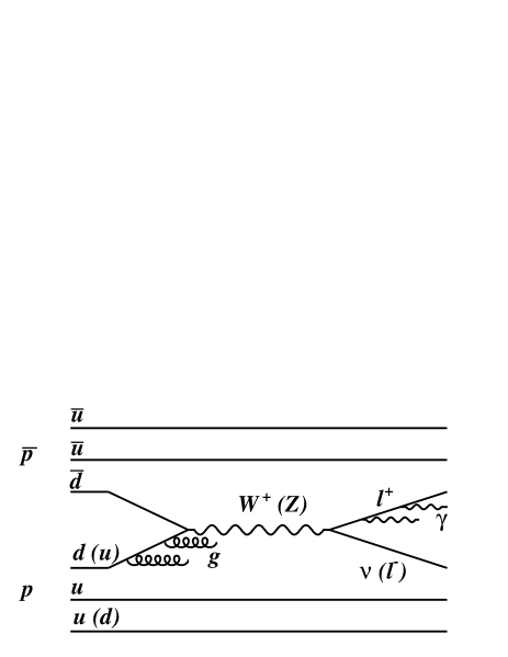
Figure 1: Quark-antiquark annihilation producing a $W$ or $Z$ boson in $p\mathrm{bar}{p}$ collisions. Higher-order processes such as initial-state gluon radiation and final-state photon radiation are also illustrated.

II.2 Definitions

The CDF experiment uses a right-handed coordinate system in which the $z$ axis is centered at the middle of the detector and points along a tangent to the Tevatron ring in the proton-beam direction. The remaining Cartesian coordinates are defined with $+x$ pointing outward and $+y$ upward from the Tevatron ring, respectively. Corresponding cylindrical coordinates are defined with $r\equiv\sqrt{x^{2}+y^{2}}$ and azimuthal angle $\phi\equiv\tan^{-1}(y/x)$. The rapidity $\zeta=-\frac{1}{2}\ln(E+p_{z}c)/(E-p_{z}c)$ is additive under boosts along the $z$ axis. In the case of massless particles, $\zeta$ equals the pseudorapidity $\eta=-\ln[\tan(\theta/2)]$, where $\theta$ is the polar angle with respect to the $z$ axis. Transverse quantities such as transverse momentum are projections onto the $x-y$ plane. The interacting protons and antiprotons have negligible net transverse momentum. Electron energy measured in the calorimeter is denoted as $E$ and the corresponding transverse momentum $E_{T}$ is derived using the direction of the reconstructed particle trajectory (track) and neglecting the electron mass. Muon transverse momentum $p_{T}$ is derived from its measured curvature in the magnetic field of the tracking system. The recoil is defined as the negative transverse momentum of the vector boson, and is measured as

$$\vec{u}_{T}=\sum_{i}E_{i}\sin(\theta_{i})\hat{n}_{i},$$ (2)

where the sum is performed over calorimeter towers (Sec. III.2), with energy $E_{i}$, tower polar angle $\theta_{i}$, and tower transverse vector components $\hat{n}_{i}\equiv(\cos\phi_{i},\sin\phi_{i})$. The tower direction is defined as the vector from the reconstructed collision vertex to the tower center. The sum excludes towers that typically contain energy associated with the charged lepton(s). We define the magnitude of $\vec{u}_{T}$ to be $u_{T}$, the component of recoil projected along the lepton direction to be $u_{||}$, and corresponding orthogonal component to be $u_{\perp}$ (Fig. 2). From $\vec{p}_{T}$ conservation, the transverse momentum of the neutrino in $W$-boson decay is inferred as $\vec{p}_{T}^{~{}\nu}\equiv-\vec{p}_{T}^{~{}\ell}-\vec{u}_{T}$, where $\vec{p}_{T}^{~{}\ell}$ is the transverse momentum of the charged lepton. We use units where $\hbar=c\equiv 1$ for the remainder of this paper.

Figure 2: Typical vectors associated to quantities reconstructed in a $W$-boson event, with the recoil hadron momentum ($\vec{u}_{T}$) separated into axes parallel ($u_{||}$) and perpendicular ($u_{\perp}$) to the charged lepton.

II.3 Measurement strategy

The measurement is performed by fitting for $M_{W}$ using three transverse quantities that do not depend on the unmeasured longitudinal neutrino momentum: $p_{T}^{\ell}$, $p_{T}^{~{}\nu}$, and the transverse mass $m_{T}=\sqrt{2p_{T}^{\ell}p_{T}^{~{}\nu}(1-\cos\Delta\phi)}$ mT , where $\Delta\phi$ is the angle between the charged lepton and neutrino momenta in the transverse plane. Candidate events are selected with $u_{T}\ll p_{T}^{\ell}$, so the neutrino momentum can be approximated as $p_{T}^{~{}\nu}\approx p_{T}^{\ell}+u_{||}$ and the transverse mass can be approximated as $m_{T}\approx 2p_{T}^{\ell}+u_{||}$. These relations demonstrate the importance of modeling $u_{||}$ accurately relative to other recoil components. They also demonstrate that the three fit variables have varying degrees of sensitivity to the modeling of the recoil and the $p_{T}$ of the $W$ boson.

High precision determination of $p_{T}^{\ell}$ is crucial to this measurement: a given fractional uncertainty on $p_{T}^{\ell}$ translates into an equivalent fractional uncertainty on $M_{W}$. We calibrate the momentum scale of track measurements using large samples of $J/\psi$ and $\Upsilon$ meson decays to muon pairs. These states are fully reconstructed as narrow peaks in the dimuon mass spectrum, with widths dominated by detector resolution. The absolute scale of the calibrated track momentum is tested by measuring the $Z$-boson mass in $Z\rightarrow\mu\mu$ decays and comparing it to the known value. After including the $M_{Z}$ measurement, the calibration is applied to the measurement of $M_{W}$ in $W\to\mu\nu$ decays and in the procedure used for the calibration of the electron energy scale in the calorimeter.

The electron energy scale is calibrated using the ratio of the calorimeter energy to track momentum ($E/p$) in $W$ and $Z$ boson decays to electrons. As with the track momentum calibration, we use a measurement of $M_{Z}$ to validate this energy calibration.

During the calibration process, all $M_{Z}$ fit results from both $ee$ and $\mu\mu$ decay channels are offset by a single unknown parameter in the range $[-75,75]$ MeV. This blinding offset is removed after the calibrations of momentum and energy scales are complete. The $M_{Z}$ measurements are then included in the final calibration.

Since $W$ and $Z$ bosons are produced from a similar initial state at a similar energy scale, the hadronic recoil is similar in the two processes. To model the detector response to this recoil, we develop a heuristic description of the contributing processes and tune the model parameters using fully-reconstructed $Z\rightarrow\ell\ell$ data. The inclusive $p_{T}$ distribution of produced $W$ bosons is also tuned using $Z\rightarrow\ell\ell$ data by combining the measured $p_{T}$ distribution of $Z$ bosons with a precise calculation resbos of the relative $p_{T}$ distributions of $W$ and $Z$ bosons.

We employ a parametrized Monte Carlo simulation to model the line shapes of the $p_{T}^{\ell}$, $p_{T}^{~{}\nu}$, and $m_{T}$ distributions. For each distribution, we generate templates with $M_{W}$ between 80 GeV and 81 GeV, and perform a binned likelihood fit to extract $M_{W}$. Using the statistical correlations derived from simulated experiments, we combine the $m_{T}$, $p_{T}^{\ell}$, and $p_{T}^{~{}\nu}$ fits from both $W\to e\nu$ and $W\to\mu\nu$ channels to obtain a final measured value of $M_{W}$.

As with the fits for $M_{Z}$, a single blinding offset in the range $[-75,75]$ MeV is applied to all $M_{W}$ fits for the course of the analysis. This offset differs from that applied to the $M_{Z}$ fits. No changes are made to the analysis once the offsets to the $M_{W}$ fit results are removed.

III The CDF II detector

The CDF II detector wzprd ; CDF2 ; jpsi is a forward-backward and cylindrically symmetric detector designed to study $p\mathrm{bar}{p}$ collisions at the Fermilab Tevatron. The structure of the CDF II detector, seen in Fig. 3, is subdivided into the following components, in order of increasing radius: a charged-particle tracking system, composed of a silicon vertex detector SVX and an open-cell drift chamber COT ; a time-of-flight measurement detector TOF ; a system of electromagnetic calorimeters CEM ; cemresponse , to contain electron and photon showers and measure their energies, and hadronic calorimeters HAD , to measure the energies of hadronic showers; and a muon detection system for identification of muon candidates with $p_{T}\gtrsim 2$ GeV. Events are selected online using a three-level system (trigger) designed to identify event topologies consistent with particular physics processes, such as $W$ and $Z$ boson production. Events passing all three levels of trigger selection are recorded for offline analysis. The major detector subsystems are described below.

Figure 3: Cut-away view of a section of the CDF II detector (the time-of-flight detector is not shown). The slice is in half the $y-z$ plane at $x=0$.

III.1 Tracking system

The silicon tracking detector consists of three separate subdetectors: L00, SVX II, and ISL SVX . The L00 detector consists of a single-sided layer of silicon wafers mounted directly on the beampipe at a radius of 1.6 cm. The SVX II detector consists of five layers of double-sided silicon wafers extending from a radius of 2.5 cm to 10.6 cm. Surrounding SVX II in the radial direction are port cards that transport data from the silicon wafers to the readout system. The outermost layer of the silicon detector, the ISL, consists of one layer of double-sided silicon at a radius of 23 cm in the central region ($|\eta|\leq 1$), and two layers of silicon at radii of 20 cm and 29 cm in the forward region ($1<|\eta|<2$).

The central outer tracking detector (COT) COT , an open-cell drift chamber, surrounds the silicon detector and covers the region $|z|<155$ cm and $40<r<138$ cm. Charged particles with $p_{T}\gtrsim 300$ MeV and $|\eta|\lesssim 1$ traverse the entire radius of the COT. The COT is segmented radially into 8 superlayers containing 12 sense-wire layers each. Azimuthal segmentation consists of 12-wire cells, such that adjacent cells’ planes are separated by $\approx 2$ cm. The detector is filled with a 1:1 argon-ethane gas mixture providing an ionization drift velocity of 56  µm/ns resulting in a maximum drift time of 177 ns. The superlayers alternate between stereo and axial configurations. The axial layers provide $r-\phi$ measurements and consist of sense wires parallel to the $z$-axis, while the stereo layers contain sense wires at a $\pm 2^{\circ}$ angle to the $z$ axis. The sense wires are held under tension from an aluminum endplate at each end of the COT in the $z$ direction (Fig. 4). The wires are azimuthally sandwiched by field sheets that provide a 1.9 kV/cm electric field.

The entire tracking system is immersed in a 1.4 T magnetic field generated by a superconducting solenoid solenoid with a length of 5 m and a radius of 1.5 m. A $\chi^{2}$ minimization procedure is used to reconstruct the helical trajectory of a charged particle using COT hit positions. The trajectory is defined in terms of five parameters: the signed transverse impact parameter with respect to the nominal beam axis $d_{0}$; the azimuthal angle at closest approach to the beam $\phi_{0}$; the longitudinal position at closest approach to the beam $z_{0}$; the cotangent of the polar angle $\cot\theta$; and the curvature $c\equiv(2R)^{-1}$, where $R$ is the radius of curvature. Individual COT hit positions are corrected for small nonuniformities of the magnetic field. Post-reconstruction corrections to the track curvature are derived using $J/\psi\to\mu\mu$, $\Upsilon\to\mu\mu$, and $W\to e\nu$ data (Sec. VII). The measured track $p_{T}$ is a constant divided by the track curvature.

Figure 4: End view of a section of a COT endplate COT . The endplates contain precision-machined slots where each cell’s sense wires and field sheets are held under tension. The radius at the center of each superlayer is shown in centimeters.

III.2 Calorimeter system

The central calorimeter is situated beyond the solenoid in the radial direction. The calorimeter has a projective-tower geometry with 24 wedges in azimuth and a radial separation into electromagnetic and hadronic compartments. Particles produced at the center of the detector with $|\eta|<1.1$ have trajectories that traverse the entire electromagnetic compartment of the central calorimeter. The calorimeter is split at $\eta=0$ into two barrels, each of which is divided into towers of size $\Delta\eta\approx 0.11\times\Delta\phi\approx 0.26$. Two neighboring towers subtending $0.77<\eta<1.0$ and $75^{\circ}<\phi<90^{\circ}$ are removed to allow a pathway for solenoid cryogenic tubes. The forward plug region of the calorimeter covers $1.1<|\eta|<3.6$ plug .

The central electromagnetic calorimeter (CEM) CEM ; cemresponse consists of 31 layers of scintillator alternating with 30 layers of lead-aluminum plates. There are $\approx 18$ radiation lengths of detector material from the collision point to the outer radius of the CEM. Embedded at a depth of $R_{CES}=184$ cm ($\approx 6X_{0}$), where electromagnetic showers typically have their maximum energy deposition, is the central electromagnetic shower-maximum detector (CES). The CES consists of multiwire proportional chambers whose anode wires measure the azimuthal coordinate of the energy deposition and whose cathodes are segmented into strips that measure its longitudinal coordinate with a position resolution of $\approx 2$ mm. The position of the shower maximum is denoted as CES $x$ (ranging from $-24.1$ cm to 24.1 cm) in the $-R_{CES}\phi$ direction and CES $z$ (ranging from $\pm 6$ cm to $\pm 239$ cm) along the $z$ axis.

The central hadronic calorimeter HAD is subdivided into a central region covering $|\eta|<0.6$ and a wall region covering $0.6<|\eta|<1.1$. The central region consists of 32 alternating layers of scintillator and steel, corresponding to 4.7 interaction lengths. The wall region consists of 15 such layers.

III.3 Muon detectors

Two sets of muon detectors separately cover $|\eta|<0.6$ and $0.6<|\eta|<1$. In the $|\eta|<0.6$ region two four-layer planar drift chambers, the central muon detector (CMU) CMU and the central muon upgrade (CMP), sandwich 60 cm of steel and are situated just beyond the central hadronic calorimeter in the radial direction. The central muon extension (CMX) is an eight-layer drift chamber providing the remaining coverage in the forward region.

III.4 Trigger system

The CDF data acquisition system collects and stores events at a rate of $\approx 100$ Hz, or about one out of every 17 000 $p\mathrm{bar}{p}$ crossings. Events are selected using a three-level system consisting of two hardware-based triggers and one software-based trigger.

The first level of triggering reconstructs charged-particle tracks, calorimeter energy deposits, and muon detector tracks (stubs). Tracks are found in the COT with a trigger track processor, the extremely-fast-tracker (XFT) XFT , using a lookup table of hit patterns in the axial superlayers. In the CMU and CMX detectors, particle momentum is estimated using the timing of signals in neighboring wires. The electron and muon triggers used in this analysis require either a calorimeter tower with electromagnetic $E_{T}>8$ GeV and a matched XFT track with $p_{T}>8$ GeV, a CMU stub with $p_{T}>6$ GeV matched to a CMP stub and an XFT track with $p_{T}>4$ GeV, or a CMX stub with $p_{T}>6$ GeV matched to an XFT track with $p_{T}>8$ GeV.

In the second trigger level, electromagnetic towers are clustered to improve energy resolution, allowing a higher threshold of $E_{T}>16$ GeV on electromagnetic clusters. The level 2 muon trigger requires both CMU and CMP stubs (a “CMUP” stub) to be matched to an XFT track with $p_{T}>8$ GeV for the majority of the data used in this analysis.

The third trigger level fully reconstructs events using an array of $\approx 300$ dual-processor computers. The electron trigger applies requirements on the distribution of energy deposited in the calorimeter and on the relative position of the shower maximum and the extrapolated COT track, as well as increased energy ($E_{T}>18$ GeV) and momentum ($p_{T}>9$ GeV) thresholds. The muon triggers require either a CMUP stub or a CMX stub to be matched to a COT track with $p_{T}>18$ GeV.

In order to model the contribution of multiple $p\mathrm{bar}{p}$ collisions to the recoil resolution, a zero bias trigger is used. This trigger randomly samples the bunch crossings without applying detector requirements. An additional minimum bias trigger collects events consistent with the presence of an inelastic collision. The trigger requires coincident signals in two small-angle gas Cherenkov luminosity counter detectors CLC arranged in three concentric layers around the beam pipe and covering $3.6<|\eta|<4.6$. These detectors are also used to determine the instantaneous luminosity of the $p\mathrm{bar}{p}$ collisions.

IV Detector simulation

The measurement of $M_{W}$ is based on a detailed custom model of the detector response to muons, electrons, photons, and the hadronic recoil. The simulation is fully tunable and provides a fast detector model at the required precision. A geant GEANT -based simulation of the CDF II detector CDFSim is also used in order to model the $Z\to\ell\ell$ background to $W\to\ell\nu$ events, where a detailed simulation of leptons outside the fiducial acceptance is required.

The fast simulation model of muon interactions includes the processes of ionization energy loss and multiple Coulomb scattering. In addition to these processes, the electron simulation contains a detailed model of bremsstrahlung. The modeled photon processes are $\gamma\rightarrow ee$ conversion and Compton scattering. This section describes the custom simulation of the above processes, the COT response to charged particles, and the calorimeter response to muons and electron and photon showers. The model of hadronic recoil response and resolution is discussed in Sec. IX.

IV.1 Charged-lepton scattering and ionization

While traversing the detector, charged leptons can undergo elastic scattering off an atomic nucleus or its surrounding electrons. The ionization of atomic electrons results in energy loss, reducing the track momentum measured in the COT. Scattering also affects the particle trajectory, thus affecting the resolution of the reconstructed track parameters.

The total energy loss resulting from many individual collisions is given by the convolution of the collision cross section over the number of target electrons bichsel . This convolution can be described by a Landau distribution,

$$L(dE)=\frac{1}{2\pi i}\int_{a-i\infty}^{a+i\infty}e^{(dE)s+s\log s}ds,$$ (3)

where $a$ is a constant, $dE$ is the total energy loss, $s=dE-\langle dE\rangle$, and $\langle dE\rangle$ is the most probable value of the energy loss pdg :

$$\langle dE\rangle=\zeta\left[\ln\left(\frac{2m_{e}\beta^{2}\gamma^{2}\zeta}{I^{2}}\right)+j-\beta^{2}-\delta\right],$$ (4)

where $\zeta=(K/2)(Z/A)(x/\beta^{2})$, $K=4\pi N_{A}r_{e}^{2}m_{e}$, $N_{A}$ is Avogadro’s number, $m_{e}$ is the electron mass, $r_{e}$ is the classical electron radius, $Z~{}(A)$ is the atomic (mass) number, $x$ is the material thickness, $j=0.2$, $\beta$ is the particle velocity, $I$ is the mean excitation energy, and $\delta$ is the material-dependent density effect as a function of $\beta$. We use silicon for the material in the calculation of $\delta$.

We calculate the total energy loss of electrons and muons in the material upstream of the COT by sampling the Landau distribution after each of 32 radial steps using a fine-grained lookup table of $\langle Z/A\rangle$ and $I$ of the detector. Within the COT we calculate the energy loss along the trajectory up to the radius of each sense wire. To obtain a measured $J/\psi$ mass that is independent of the $\langle p_{T}^{-1}\rangle$ of the final-state muons, we multiply the energy loss upstream of the COT by a correction factor of 1.043, as described in Section VII.2.

The effect of Coulomb scattering on each particle’s trajectory is modeled by a Gaussian distribution of the scattering angle through each radial step of the detector. For 98% of the scatters ms , the core Gaussian resolution is

$$\sigma_{\vartheta}=\frac{13.6~{}{\rm MeV}}{\beta p}\sqrt{x/X_{0}},$$ (5)

where $x$ is the thickness of the layer and $X_{0}$ is the layer’s radiation length CDF2 ; tsai . The remaining 2% of the scatters are modeled by a Gaussian with resolution $3.8\sigma_{\vartheta}$, based on results of low-energy muon scattering data mstail .

IV.2 Electron bremsstrahlung

Bremsstrahlung radiation is modeled using the Bethe-Heitler spectrum CDF2 ; tsai

$$\frac{d\sigma}{dy}=\frac{A}{N_{A}X_{0}\rho}\left[\left(\frac{4}{3}+C\right)\left(\frac{1}{y}-1\right)+y\right],$$ (6)

where $\rho$ is the material density, $y$ is the fraction of the electron momentum carried by the photon, and $C$ is a material-dependent constant (taken to be 0.02721, the value appropriate for copper). The spectrum receives corrections riddick for the suppression of photons radiated with very low or high $y$. For $y\gtrsim 0.8$, the nuclear electromagnetic field is not completely screened by the atomic electrons tsai , reducing the bremsstrahlung cross section. For $y\lesssim 0.05$, interference effects from multiple Coulomb migdal or Compton dielectric scattering reduce the rate of photon radiation. The Landau-Pomeranchuk-Migdal (LPM) suppression due to multiple Coulomb scattering is given in terms of the Bethe-Heitler cross section as

$$S_{LPM}\equiv\frac{d\sigma_{LPM}/dy}{d\sigma_{BH}/dy}=\sqrt{\frac{E_{LPM}}{E_{e}}\frac{y}{(1-y)}},$$ (7)

where $E_{LPM}$ depends on the material traversed by the electron. Dense materials have low $E_{LPM}$ and more significant suppression.

We model the material dependence of the LPM effect based on the material composition of the upstream detector, whose components were determined at the time of construction to a relative accuracy of 10%. To simplify the model, the low-density and high-density components are each modeled as a single element or mixture in each layer. The relative fractions of the low-density and high-density components are determined by the ionization energy-loss constant and the radiation lengths of the layer. In increasing radius, the upstream material is modeled as follows: a beryllium beampipe; silicon sensors mounted on hybrid readout structures consisting of a low-density mixture of equal parts beryllium oxide and glass, combined with gold; portcards consisting of a low-density mixture of 37% beryllium oxide and 63% kapton combined with a high-density mixture of 19% gold and 81% copper; the carbon inner COT wall; and the COT active volume consisting of kapton combined with a high-density mixture of 35% gold and 65% copper. The main feature in the longitudinal direction is the silicon beryllium bulkhead located at $z=\pm 15$ cm and $\pm 45$ cm. The model of simplified components is designed to reproduce the measured components to a relative accuracy of 10%.

In each traversed layer we calculate the number of photons radiated using the integrated Bethe-Heitler spectrum. For each photon we draw a value of $y$ from this spectrum and apply the appropriate radiation suppression CDF2 if $y$ is outside the range 0.05 to 0.8.

IV.3 Photon conversion and scattering

Photons radiated in the production and the decay of the $W$ boson, or in the traversal of electrons through the detector, contribute to the measured electron energy if the photon shower is in the vicinity of the electron shower. This contribution depends on photon conversions and on photon scattering in the material upstream of the calorimeter. We model these interactions explicitly at radii less than that of the outer COT wall.

The probability for a photon to convert depends on the photon energy and on the number of radiation lengths traversed. At high photon energy the probability is determined by integrating the screened Bethe-Heitler equation tsai ; CDF2 over the fraction $y$ of photon energy carried by the conversion electron. The dependence of this probability on photon energy has been tabulated in detail hubble ; we parametrize this dependence to determine the conversion probability of a given photon in the detector CDF2 .

To account for the internal-conversion process, where an incoming electron produces three electrons via an internal photon, we add an effective number of radiation lengths due to the photon-conversion coupling, $\Delta(x/X_{0})=(\alpha_{\mathrm{EM}}/\pi)\log(E_{\gamma}/m_{e})$ photonsplit . The radius of conversion is chosen using the radial distribution of radiation lengths. The energy fraction $y$ is taken from the Bethe-Heitler spectrum.

Compton scattering reduces the photon energy and is relevant at low photon momentum. We parametrize the cross section using the tables in Ref. hubble and apply a fractional energy loss ($y$) distribution according to $d\sigma/dy\propto 1/y+y$, using a lower bound of $y=0.001$ CDF2 .

IV.4 COT simulation and reconstruction

The track simulation produces individual measurement points (hits) in the COT based on the trajectory of each charged lepton in the generated event CDF2 . The hit spatial resolution is determined for each superlayer using the reconstructed muon tracks in $Z\rightarrow\mu\mu$ data, with global multiplicative factors chosen to best match the mass distributions of the calibration resonances in data. These factors deviate from one by $\lesssim 5\%$. The resolution improves from $\approx 180$  µm in the inner superlayer to $\approx 140$  µm in the outer superlayer. Efficiencies for detecting hits are tuned to approximate the hit multiplicity distribution of the leptons in each sample CDF2 . A small correlated hit inefficiency in the inner superlayers accounts for the effects of high occupancy. For prompt lepton candidates the transverse beam position is added as a constraint in the track fit, with the $42\pm 1_{\rm stat}~{}$ µm beam size chosen to minimize the $\chi^{2}$ of the reconstructed $Z\rightarrow\mu\mu$ mass distribution.

IV.5 Calorimeter response

Between the outer COT wall and the outer radius of the electromagnetic calorimeter there are $\approx 19$ radiation lengths of material. Using a detailed geant model of this material, we parametrize the calorimeter response to electrons and photons as a function of energy and traversed radiation lengths calgeantnim . The parametrization models the longitudinal leakage of the shower into the hadronic calorimeter, the fraction of energy deposited in the scintillators (including fluctuations), and the energy dependence of the response due to the material upstream of the scintillators and to the lead absorbers.

The measured transverse energy $E_{T}^{\rm meas}$ is parametrized as

$$E_{T}^{\rm meas}=S_{E}\left(1+\xi\log\frac{E_{T}^{\rm inc}}{39~{}{\rm GeV}}\right)E_{T}^{\rm inc},$$ (8)

where $E_{T}^{\rm inc}$ is the incident transverse energy, the empirical correction $\xi$ accounts for the depth dependence of the calorimeter response due to aging or attenuation in the light guides, and $S_{E}$ is the energy scale determined using the same data (see Sec. VIII). The measured energy receives corrections dependent on the measured CES position of the electron shower CDF2 . The correction $\xi=(5.25\pm 0.70_{\rm stat})\times 10^{-3}$ is determined using the observed energy dependence of the electron response in $W$ and $Z$ boson data. This correction is adjusted for photons, which produce an electromagnetic shower deeper in the calorimeter, by simulating conversion of the photon at an average depth and applying the appropriate correction to each conversion electron.

Electrons and photons in the same tower, and those in the closest tower in $\eta$, are combined to produce a calorimeter electron cluster. A Gaussian smearing is applied to the energy of this cluster with fractional resolution $\sigma_{E}/E=\sqrt{0.126^{2}/E_{T}+\kappa^{2}}$, where $E_{T}$ is in GeV and $\kappa=[0.58\pm 0.05$(stat)$]\%$ is determined by minimizing the $\chi^{2}$ of the $E/p$ distribution of electrons from the $W$-boson data sample. To model the resolution of the $Z\rightarrow ee$ mass peak for electrons radiating a high-momentum photon, i.e., those electrons with $E/p>1.11$, we apply an additional constant term of $\kappa_{\gamma}=[7.4\pm 1.8]\%$ to all radiated photons and electrons within the simulated electron cluster. Electron showers in the two towers nearest $|\eta|=0$ can leak into the gap between the central calorimeters. The resulting loss in energy degrades the measurement resolution of the cluster. To account for this degradation, an additional constant term of $\kappa_{0}=0.96\%$ is added in quadrature to $\kappa$ for these two towers.

To improve the modeling of the low tail of the $E/p$ distribution for electrons, which is typically populated by electron showers with high leakage out of the electromagnetic calorimeter, we multiply the nominal radiation lengths of the calorimeter by a pseudorapidity-dependent value between 1 and 1.027. We improve the modeling of the high tail of the $E/p$ distribution for electrons, typically populated by electrons with significant photon radiation in the material upstream of the COT, by multiplying the nominal radiation lengths of this material by 1.026.

The energy deposited by muons in the calorimeter is simulated using a distribution from identified cosmic rays with no additional tracks in the event CDF2 . The underlying event contribution is modeled from the observed distribution in $W$-boson data and scaled to account for its dependence on $u_{||}$, $u_{\perp}$, and tower $\eta$. The distribution is determined using towers at a wide angle relative to the lepton in the event and is thus sensitive to the lower threshold on tower energy of 60 MeV, which is easily exceeded in a tower traversed by a high-momentum lepton. To correct for this threshold bias we add 25 MeV to the underlying event energy in the lepton calorimeter towers, where 25 MeV is the mean energy of the extrapolated observed distribution below 60 MeV.

V Production and decay models

The $W$-boson mass is extracted from fits to kinematic distributions, requiring a comprehensive theoretical description of boson production and decay. We describe the production of $W$ and $Z$ bosons using CTEQ6.6 parton distribution functions (PDFs) CTEQ and the resbos generator resbos , which combines perturbative QCD with a parametrization of nonperturbative QCD effects. The parameters are determined in situ with fits to $Z$-boson data. The boson polarization is accounted for perturbatively in QCD when modeling the boson decay. Radiation of photons from the final-state charged lepton is simulated using the photos photos generator and calibrated to the horace horace generator for the $M_{W}$ and $M_{Z}$ mass measurements.

V.1 Parton distribution functions

At the Tevatron the longitudinal momentum of a given $W$ or $Z$ boson is unknown, but its distribution is well constrained by the parton distribution functions (PDFs) describing the fraction $x_{i}$ of a hadron’s momentum carried by a given interacting parton. We consider two independent PDF parametrizations performed by the CTEQ CTEQ and MSTW MSTW collaborations.

The mass measurement is performed using the next-to-leading-order CTEQ6.6 parton distribution functions to model the parton momentum fraction in $p\mathrm{bar}{p}$ collisions. Variations in the PDFs affect the lepton acceptance as a function of the lepton’s decay angle with respect to the beam axis. Since the $W$-boson mass is measured using transverse quantities, this change in acceptance impacts the measurement. The CTEQ and MSTW collaborations independently determine a set of eigenvectors to form an orthonormal basis, from which uncertainties due to PDF variations can be calculated. The sets calculated by the CTEQ collaboration correspond to 90% C.L. uncertainty, while the sets calculated by the MSTW collaboration correspond to both 90% C.L. and 68% C.L. uncertainties. We calculate the total PDF uncertainty on $M_{W}$ from a quadrature sum of all eigenvector contributions in a given set of eigenvectors, $\delta M_{W}^{\mathrm{PDF}}=\frac{1}{2}\sqrt{\sum_{i}(M_{W}^{i+}-M_{W}^{i-})^{2}},$ where $M_{W}^{i\pm}$ represents the fitted mass obtained using the $\pm n\sigma$ shifts in the $i$th eigenvector. In the cases where the signs of $M_{W}^{i+}$ and $M_{W}^{i-}$ are the same, we use half the maximum deviation between the nominal $M_{W}$ and $M_{W}^{i+}$ or $M_{W}^{i-}$. Using events generated with horace horace , we find $\delta M_{W}$ to be consistent between the CTEQ6.6 and MSTW2008 PDF 90% C.L. sets. We calculate the systematic uncertainty due to PDFs using the 68% C.L. eigenvectors for the MSTW2008 PDF sets and obtain $\delta M_{W}$ of 10, 9, and 11 MeV for the $m_{T}$, $p_{T}^{\ell}$, and $p_{T}^{\nu}$ fits, respectively zeng ; beecher . As a consistency check we find that fits using the nominal CTEQ6.6 and MSTW2008 PDF sets yield $M_{W}$ values that differ by 6 MeV.

V.2 $W$ and $Z$ boson $p_{T}$

The $p_{T}$ of the $W$ boson affects the kinematic distributions used to fit for $M_{W}$, particularly the distribution of charged lepton $p_{T}$. We model the $p_{T}$ of the vector boson $V$ using the resbos generator, which merges a fixed-order perturbative QCD calculation at large boson $p_{T}$ with a resummed perturbative QCD calculation at intermediate $p_{T}$ and a nonperturbative form factor at low $p_{T}$. resbos uses the Collins-Soper-Sterman css resummation formalism to describe the cross section for vector-boson production as

$$\begin{split}\frac{d\sigma(jk\rightarrow V+X)}{d\hat{s}d^{2}\vec{p}_{T}^{~{}V}dy}&\propto\int d^{2}\vec{b}e^{i\vec{p}_{T}^{~{}V}\cdot\vec{b}}\\ &\times\tilde{W}_{jk}(\vec{b},\hat{s},x_{j},x_{k})\times e^{-S}+Y_{jk}(p_{T}^{V},\hat{s},x_{j},x_{k}),\end{split}$$ (9)

where $\sqrt{\hat{s}}$ is the partonic center-of-mass energy, $y$ is the boson rapidity, $x_{j}$ and $x_{k}$ are the momentum fractions of partons $j$ and $k$, respectively, and $\vec{b}$ is the relative impact parameter of the partons in the collision. The functions $\tilde{W}_{jk}$ and $Y_{jk}$ are perturbative terms, while $S$ parametrizes the nonperturbative part of the transition amplitude. resbos uses the Brock-Landry-Nadolsky-Yuan form to characterize the nonperturbative function as resbos

$$S=\Bigg{[}g_{1}-g_{2}\log\Bigg{(}\frac{\sqrt{\hat{s}}}{2Q_{0}}\Bigg{)}-g_{1}g_{3}\log(100x_{j}x_{k})\Bigg{]}b^{2},$$ (10)

where $Q_{0}$ is the cutoff parameter of 1.6 GeV and $g_{1}$, $g_{2}$, and $g_{3}$ are parameters to be determined experimentally. At fixed beam energy and $\hat{s}$, the $g_{i}$ parameters are completely correlated beecher . The parameter $g_{2}$ is particularly sensitive to the position of the peak of the boson $p_{T}$ spectrum. We fit for $g_{2}$ using the dilepton $p_{T}$ spectra from $Z\to ee$ and $Z\to\mu\mu$ candidate events (Fig. 5), obtaining a statistical uncertainty on $g_{2}$ of 0.013 GeV² g2value . We vary $g_{3}$ by $\pm 0.3$ (the uncertainty obtained in a global fit resbos ) and find that this variation is equivalent to a $g_{2}$ variation of $\pm 0.007$ GeV². Thus, the combined effective uncertainty on $g_{2}$ is $\pm 0.015$ GeV², which translates to uncertainties on $M_{W}$ of 1, 3, and 2 MeV for the $m_{T}$, $p_{T}^{\ell}$, and $p_{T}^{\nu}$ fits, respectively.

The boson $p_{T}$ spectrum is sensitive to the value of the strong-interaction coupling constant $\alpha_{s}$, particularly at high boson $p_{T}$ ($\gtrsim 5$ GeV). We parametrize the variation of the boson $p_{T}$ spectrum with $\alpha_{s}$ variations in resbos and use this parametrization to propagate the constraint from the dilepton $p_{T}$ spectra to an uncertainty on $M_{W}$. The resulting uncertainties on $M_{W}$ are 3, 8, and 4 MeV for the $m_{T}$, $p_{T}^{\ell}$, and $p_{T}^{\nu}$ fits, respectively.

We perform a simultaneous fit of the data to $g_{2}$ and $\alpha_{s}$ and determine their correlation coefficient to be $-0.71$ beecher . Including this anticorrelation, the uncertainties on $M_{W}$ due to the modeling of the $p_{T}^{W}$ distribution are 3, 9, and 4 MeV for the $m_{T}$, $p_{T}^{\ell}$, and $p_{T}^{\nu}$ fits, respectively.

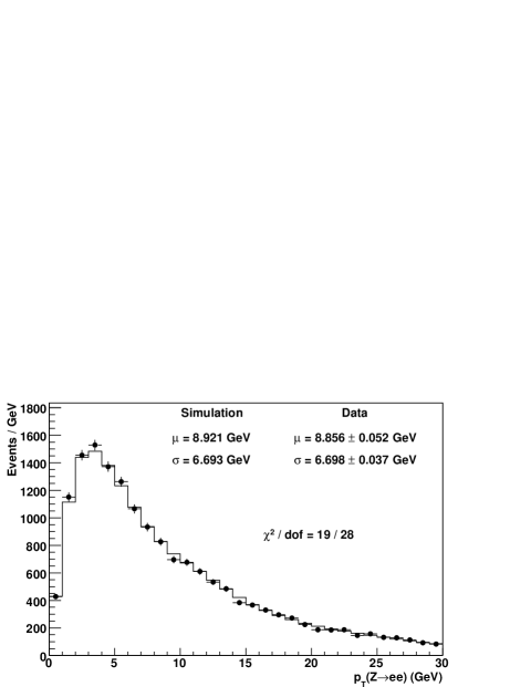
Figure 5: Distributions of $p_{T}^{Z}$ from simulation (histogram) and data (circles) for $Z$-boson decays to $\mu\mu$ (top), and to $ee$ (bottom). The distributions are used to fit for the nonperturbative parameter $g_{2}$ and for $\alpha_{s}$.

V.3 Boson decay

The polarization of a vector boson produced in proton-antiproton collisions is affected by the initial-state QCD radiation associated with the boson production. This polarization, together with the $V-A$ coupling of the weak interactions, determines the angular distributions of the final-state leptons in the vector-boson rest frame. resbos models the boson polarization to next-to-next-to-leading-order (NNLO) in $\alpha_{s}$.

We validate the resbos prediction by comparing the angular distribution of the charged lepton to that predicted by the NLO $W+\geq 1$-jet generator dyrad dyrad . Using the Collins-Soper frame cs , defined as the rest frame of the $W$ boson with the $x$ axis along the direction of $p_{T}^{W}$, the angular distribution of the charged lepton is expressed as

$$\begin{split}\frac{d\sigma}{d\Omega}\propto&(1+\cos^{2}\theta)+\frac{1}{2}A_{0}(1-3\cos^{2}\theta)\\ &+A_{1}\sin 2\theta\cos\phi+\frac{1}{2}A_{2}\sin^{2}\theta\cos 2\phi\\ &+A_{3}\sin\theta\cos\phi+A_{4}\cos\theta+A_{5}\sin^{2}\theta\sin 2\phi\\ &+A_{6}\sin 2\theta\sin\phi+A_{7}\sin\theta\sin\phi,\end{split}$$ (11)

where the coefficients $A_{i}$ are calculated to NNLO in $\alpha_{s}$ as functions of $p_{T}^{W}$. We compare each $A_{i}(p_{T}^{W})$ value obtained from resbos with that from dyrad and find the generators to give consistent coefficients for $p_{T}^{W}>50$ GeV. At lower $p_{T}^{W}$ the coefficients from resbos evolve continuously to the expected behavior for $p_{T}^{W}\to 0$, since resbos includes the QCD resummation calculation at low $p_{T}^{W}$, while dyrad is a fixed-order calculation whose result does not asymptotically approach the expected behavior at $p_{T}^{W}=0$.

To check the effect of the difference between the fixed-order and resummed calculation on a measurement of $M_{W}$, we reweight the resbos events such that the $A_{i}$ values from resbos match the values from dyrad at $p_{T}^{W}=25$ GeV. Fitting the reweighted events with the default resbos templates results in a change in the fitted $W$-boson mass of 3 MeV. Since the resbos model includes the resummation calculation while dyrad does not, the uncertainty in the resbos model of the decay angular distribution is considered to be negligible.

V.4 QED radiation

Final-state photon radiation (FSR) from the charged lepton produced in the $W$-boson decay reduces the lepton’s momentum, biasing the measurement of $M_{W}$ in the absence of an FSR simulation. For small-angle radiation ($\Delta R\lesssim 0.1$, where $\Delta R\equiv\sqrt{(\Delta\phi)^{2}+(\Delta\eta)^{2}}$), the photon energy is recovered by the reconstruction of the electron energy in the calorimeter; for radiation at wide angles, or from muons, the photon energy is not included in the measured lepton energy.

To simulate FSR, we use the photos photos generator with an energy cutoff of $E_{\gamma}>0.4$ MeV. photos uses a leading-log calculation to produce $n$ final-state photons, with a reweighting factor applied to each photon such that the complete NLO QED calculation is reproduced for $n=1$. Ordering the photons in $p_{T}$, we include $n\leq 4$ in the event generation. Raising the $E_{\gamma}$ threshold to $4$ MeV shifts the value of $M_{W}$ fitted in pseudoexperiments by 2 MeV, which is taken as a systematic uncertainty on the choice of $E_{\gamma}$ threshold.

The simulation of QED radiation is improved with a calibration to the horace generator horace . horace performs a similar leading-log reweighting scheme to photos, but matches single-photon radiation to the NLO electroweak calculation wgrad and includes initial-state radiation (ISR) and interference between ISR and FSR. Fitting for $M_{W}$ in simulated horace events yields a shift of $-3\pm 4_{\textrm{MC stat}}$ MeV in the electron channel and $4\pm 4_{\textrm{MC stat}}$ MeV in the muon channel. We apply these corrections in the data $M_{W}$ fit. Residual uncertainties on the horace simulation of radiated photons are estimated to be 1 MeV on the $M_{W}$ measurement.

A higher-order process contributing to QED energy loss is the radiation of an electron-positron pair. To model this process, we use the effective radiator approximation photonsplit to simulate the conversion of radiated photons with a probability $(\alpha_{\mathrm{EM}}/\pi)\log(E_{\gamma}/m_{e})$; we estimate the remaining uncertainty on $M_{W}$ to be 1 MeV. The combined uncertainty on $M_{W}$ due to QED radiation is 4 MeV and is correlated between the channels and the fit distributions.

VI $W$ and $Z$ boson event selection

$W$ and $Z$ boson candidate events are selected by triggers that require a muon (electron) with $p_{T}>18$ ($E_{T}>18$) GeV (see Sec. III.4). Events in the $W$-boson sample contain one identified lepton and the following kinematic selection: $u_{T}<15$ GeV, $30<p_{T}^{\ell}<55$ GeV, $30<p_{T}^{\nu}<55$ GeV, and $60<m_{T}<100$ GeV. Candidate $Z$-boson events have two oppositely charged same-flavor identified leptons with invariant mass $m_{\ell\ell}$ in the range $66<m_{\ell\ell}<116$ GeV, and with $p_{T}(Z\to\ell\ell)<30$ GeV. Common lepton identification criteria are used in the $W$- and $Z$-boson selection. To suppress the contribution of $Z$-boson decays to the $W$-boson sample, loosened lepton identification criteria are used to reject events with additional leptons in this sample. The number of candidate events in each sample is shown in Table 1. In the following we describe the selection criteria and efficiencies for electron and muon candidates.

Table 1: Number of events passing all selection criteria for $W$ and $Z$ boson candidates in the data.

Sample	Candidate events
$W\to\mu\nu$	624 708
$W\to e\nu$	470 126
$Z\to\mu\mu$	59 738
$Z\to ee$	16 134

VI.1 Muon selection

Muon reconstruction is based on high-momentum tracks reconstructed in the COT, with muon-chamber track stubs required when necessary for consistency with trigger selection. The selection ensures high-resolution COT tracks, with high purity achieved via tracking and calorimeter quality requirements.

A large number of position measurements in multiple COT superlayers leads to high precision of the measured track parameters. We require at least five hits in three or more axial superlayers, and a total of 25 hits or more in all axial superlayers. These requirements are also applied to the hits in stereo superlayers. To suppress the potentially large background from the decays of long-lived hadrons such as $K$ or $\pi$ mesons to muons, or decays-in-flight (DIF), we impose requirements on the transverse impact parameter ($|d_{0}|<0.1$ cm) and the quality of the track fit ($\chi^{2}/$dof$<3$). In addition, we identify hit patterns characteristic of a kink in the apparent trajectory, due to a particle decay. A kinked trajectory typically leads to significant numbers of consecutive hits deviating from the helical fit in the same direction, since the trajectory is a combination of two helices. We require the number of transitions of hit deviations from one side of the track to the other to be larger than $30+2\chi^{2}/$dof, where dof is the number of degrees of freedom.

Tracks associated with muon candidates are required to originate from the luminous region ($|z_{0}|<60$ cm) and to have $p_{T}>30$ GeV, measured including a constraint to the transverse position of the beam. The tracks are geometrically extrapolated to the calorimeter and muon detectors. The total energy $E_{\rm EM}$ measured in the electromagnetic towers traversed by the extrapolated track is required to be less than 2 GeV; the peak from minimum ionization is about 350 MeV. Similarly, the total energy $E_{\rm had}$ in traversed hadronic towers is required to be less than 6 GeV, where the typical energy from minimum-ionizing particles is about 2 GeV. Candidate COT tracks are matched to muon track stubs if the $r-\phi$ distance between the extrapolated track and the stub is less than 3 cm in the CMX detector, or 5 cm and 6 cm in the CMU and CMP detectors, respectively.

To reduce the background of $Z/\gamma^{*}\to\mu\mu$ events in the $W$-boson candidate sample, we reject events with a second muon candidate satisfying either the above criteria or the following criteria, which are independent of the presence of a muon-chamber stub: $p_{T}>20$ GeV, track $\chi^{2}/$dof $<3$, $|d_{0}|<0.1$ cm, $\geq 2$ axial and $\geq 2$ stereo superlayers with $\geq 5$ hits each, $E_{\rm EM}<2$ GeV, $E_{\rm had}<6$ GeV, and $z_{0}$ within 5 cm of the candidate muon from the $W$-boson decay. Cosmic-ray background is highly suppressed by fitting for a single track crossing the entire diameter of the COT, with sets of azimuthally opposed hits cosmic .

The muon identification efficiency depends on the projection of the recoil along the direction of the muon ($u_{||}$). Large $u_{||}$ is typically associated with significant hadronic activity in the vicinity of the muon, affecting muon identification. We model this dependence through an explicit model of $E_{\rm EM}$, as described in Sec. IV.5, and a $u_{||}$-dependent efficiency measurement in data for the remaining identification requirements. This measurement uses $Z\to\mu\mu$ events with low recoil $(u_{T}<15$ GeV) and one muon passing the candidate criteria and a second probe muon identified as a track with $p_{T}>30$ GeV and $E_{\rm EM}<2$ GeV. The two muons are required to have opposite charge and an invariant mass in the range $81<m_{\ell\ell}<101$ GeV. The small background is subtracted using same-charge muon pairs. The fraction of probe muons passing the full $W$-boson muon-candidate criteria as a function of $u_{||}$ is shown in Fig. 6. We characterize the observed dependence on $u_{||}$ using the parametrization

$$\epsilon_{u}=a[1+b(u_{||}+|u_{||}|)],$$ (12)

where $a$ is a normalization parameter and $b$ is a slope parameter for $u_{||}>0$. Based on this measurement we simulate a muon identification efficiency with $b=[-0.17\pm 0.07_{\rm stat}]\times 10^{-3}$. The value of $a$ does not impact the $M_{W}$ measurement. The statistical uncertainty on $b$ results in an uncertainty $\delta M_{W}$ of 1 MeV and 2 MeV for the $p_{T}^{\ell}$ and $p_{T}^{\nu}$ fits, respectively. The uncertainty on the $m_{T}$ fit is negligible.

Figure 6: Muon identification efficiency as a function of the recoil component in the direction of the muon ($u_{||}$).

VI.2 Electron selection

Electron candidates are reconstructed from the energy deposited in a pair of EM calorimeter towers neighboring in $\eta$ and matched to a COT track extrapolated to the position of the shower maximum. Electromagnetic showers are required to be loosely consistent with that of an electron and to be fully within the fiducial volume of the EM calorimeter, based on the electron track trajectory.

Measurements of CES deposits are used to determine the energy-weighted $\phi-z$ position of the electron shower maximum. The cluster position must be separated from the edges of towers: $|\textrm{CES }x|<18$ cm, CES $z$ more than 1.58 cm from each tower edge, and CES $z$ more than 11 cm from the central division between east and west calorimeters. Requiring the shower to be fully within the fiducial volume of the EM calorimeter removes additional electron candidates in regions near $|\eta|=0$ and beyond $|\eta|=0.9$. We require electron $E_{T}>30$ GeV, where the energy is measured using the electromagnetic calorimeter and the direction is determined using the associated track.

Tracks matched to electromagnetic clusters must be fully within the fiducial volume of the COT and must pass the same hit requirements as imposed on muon tracks (see Sec. VI.1). The difference in $z$ between the extrapolated track and the cluster is required to be less than 5 cm. The track must have $p_{T}>18$ GeV and the ratio of calorimeter energy to track momentum, $E/p$, is required to be less than 1.6; this requirement significantly reduces the misidentified hadron background.

Misidentified hadrons are further suppressed with loose lateral and longitudinal shower shape requirements. The ratio of energy in the hadronic calorimeter to that in the electromagnetic calorimeter, $E_{\rm had}/E_{\rm EM}$, must be less than 0.1. A lateral shower discriminator quantifying the difference between the observed and expected energies in the two electron towers is defined as wzrun1

$$L_{\mathrm{shr}}=0.14\sum_{i}\frac{E_{i}^{\mathrm{adj}}-E_{i}^{\mathrm{exp}}}{\sqrt{0.14^{2}E_{i}^{\mathrm{adj}}+(\Delta E_{i}^{\mathrm{exp}})^{2}}},$$ (13)

where $E_{i}^{\mathrm{adj}}$ is the energy in a neighboring tower, $E_{i}^{\mathrm{exp}}$ is the expected energy contribution to that tower, $\Delta E_{i}^{\mathrm{exp}}$ is the rms spread of the expected energy, and the sum is over the two towers. All energies are measured in GeV. We require $L_{\mathrm{shr}}<0.3$.

Candidate events for the $W\to e\nu$ sample are required to have one electron satisfying the above criteria. The $Z/\gamma^{*}\to ee$ process is highly suppressed by the $u_{T}<15$ GeV requirement. Further suppression is achieved by rejecting events that have an additional high-$p_{T}$ track extrapolating to a crack between electromagnetic towers ($|\textrm{CES }x|>21$ cm, $|\textrm{CES }z|<6$ cm, or $|\textrm{CES }z|>235$ cm). The track must also have $p_{T}>20$ GeV, $|d_{0}|<0.3$ cm, and track isolation fraction less than 0.1, in order for the event to be rejected. The track isolation fraction is defined as the sum of track $p_{T}$ contained in a cone $\sqrt{(\Delta\eta)^{2}+(\Delta\phi)^{2}}=0.4$ surrounding (and not including) the candidate track, divided by the candidate track $p_{T}$.

Figure 7: Trigger efficiency as a function of track $\eta$ for electrons identified in the calorimeter.

The efficiency for reconstructing electrons is dependent on $\eta$ due to the track trigger requirements. The efficiency is measured using $W$-boson events collected with a trigger with no track requirement, and modeled using the sum of two Gaussian distributions (Fig. 7). The drop in efficiency as $|\eta|$ decreases is due to the presence of structural supports for the COT wires near $z=0$. The peak at $|\eta|=0$ arises because the gap between calorimeters overlaps with these supports, so measured electrons at $|\eta|=0$ do not traverse the supports.

As with the muon identification, the electron identification has a $u_{||}$-dependent efficiency. We measure this efficiency using a sample of $Z\to ee$ events with $u_{T}<15$ GeV where one electron passes the $W$-boson candidate criteria and the other probe electron has an EM energy cluster with $E_{T}>30$ GeV, an associated track with $p_{T}>18$ GeV, and $E/p<1.6$. The two electrons must have opposite charge and an invariant mass in the range $81<m_{\ell\ell}<101$ GeV; background is subtracted using same-charge electrons. The fraction of probe electrons passing the full $W$-boson electron-candidate criteria as a function of $u_{||}$ is shown in Fig. 8. We characterize the observed dependence on $u_{||}$ using the parametrization in Eq. (12) and apply it in the simulation with $b=(-0.20\pm 0.10)\times 10^{-3}$. The statistical uncertainty on $b$ results in uncertainties $\delta M_{W}$ of 3 MeV and 2 MeV for the $p_{T}^{\ell}$ and $p_{T}^{\nu}$ fits, respectively. The uncertainty on the $m_{T}$ fit is negligible.

Figure 8: Electron identification efficiency as a function of the recoil component in the direction of the electron ($u_{||}$).

VII Muon momentum measurement

The momentum of a muon produced in a $p\mathrm{bar}{p}$ collision is measured using a helical track fit to the hits in the COT, with a constraint to the transverse position of the beam for promptly produced muons CDF2 . The initial momentum calibration has an uncertainty determined by the precision on the average radius of the COT and on the average magnetic field. To maximize precision, we perform an additional momentum calibration with data samples of $J/\psi$ and $\Upsilon(1S)$ meson decays, and $Z$-boson decays to muons. Uniformity of the calibration is significantly enhanced by an alignment of the COT wire positions using cosmic-ray data.

VII.1 COT alignment

The nominal positions of the COT wires are based on measurements of cell positions during construction, a finite element analysis of endplate distortions due to the load of the wires, and the expected wire deflection between endplates due to gravitational and electrostatic effects COT . An alignment procedure CDF2 using cosmic-ray data taken during Tevatron proton-antiproton bunch crossings improves the accuracy of the relative positions of the wires. The procedure determines relative cell positions at the endplates using the differences between measured and expected hit positions using a single-helix track fit through the entire COT for each cosmic-ray muon cosmic . The deflection of the wires from endplate to endplate is determined by comparing parameters of separate helix fits on opposite sides of the beam axis for each muon.

The cosmic-ray sample is selected by requiring no more than two tracks from the standard reconstruction. A single-helix track fit is then performed, and fit-quality and kinematic criteria are applied. The sample used for the alignment consists of 136 074 cosmic-ray muons, weighted such that muons with positive and negative charge have equal weight. Using differences between the expected and measured hit positions, the tilt and shift of every twelve-wire cell is determined for each endplate (see Fig. 9). Constraints are applied to prevent a global rotation of the endplates and a relative twist between endplates.

Figure 9: Definitions of the tilt ($\Delta\tau$) and shift ($R\Delta\phi$) corrections derived for each twelve-wire COT cell using cosmic-ray data.

To reduce biases in track parameters as a function of $z_{0}$, a correction is applied to the nominal amplitude of the electrostatic deflection of the wires from endplate to endplate. The correction is a quadratic function of detector radius, with separate coefficients for axial and stereo superlayers.

The cosmic-ray-based alignment is used in the track reconstruction and validated with tracks from electrons and positrons from $W$-boson decays. Global misalignments to which the cosmic rays are insensitive are corrected at the track level using the difference in $\langle E/p\rangle$ between electrons and positrons, where $E/p$ is in the range 0.9–1.1. Additive corrections are applied to $q/p_{T}$, a quantity proportional to the track’s curvature, where $q$ is the particle charge. The corrections take the form

$$q\Delta p_{T}^{-1}=f(\theta)+g(\phi)+h(\theta,\phi),$$ (14)

with

$$f(\theta) = A+B\cot\theta+C\cot^{2}\theta,$$ (15)

$$g(\phi) = a_{i}\sin(\phi-\alpha_{i})+b\sin(3\phi-\beta),$$ (16)

$$h(\theta,\phi) = d\sin(\phi-\delta)\cot\theta+e\sin(3\phi-\epsilon)\cot^{2}\theta.$$ (17)

The measured values of the parameters in Eqs. (15)–(17) are shown in Table 2, with the coefficient and phase of the sinusoidal term separated approximately into the first ($a_{1}$, $\alpha_{1}$) and second ($a_{2}$, $\alpha_{2}$) halves of the collected sample. None of the other parameters show significant variation between the two halves of the data sample. The quoted uncertainties on the corrections are given by the statistical uncertainties on the data. The differences in $\langle E/p\rangle$ between positrons and electrons as functions of $\phi$ and $\cot\theta$ are shown in Fig. 10, before and after corrections. The coefficients for the correlated terms are determined using the $\langle E/p\rangle$ difference as a function of $\cot\theta$ in four equal ranges of $\phi$ centered on 0, $\pi/2$, $\pi$, and $3\pi/2$.

Table 2: Values of the correction parameters measured using the difference in $\langle E/p\rangle$ between positrons and electrons as functions of $\cot\theta$ and $\phi$. The uncertainties on the phase parameters ($\alpha_{i},\beta,\delta,\epsilon$), which are quoted in radians, have a negligible impact on the overall uncertainty due to misalignment.

Parameter	Value
$A$	$-(12\pm 8)\times 10^{-6}$ GeV-1
$B$	$-(91\pm 5)\times 10^{-6}$ GeV-1
$C$	$-(57\pm 13)\times 10^{-6}$ GeV-1
$a_{1}$	$(70\pm 70)\times 10^{-6}$ GeV-1
$\alpha_{1}$	1.3
$a_{2}$	$-(43\pm 43)\times 10^{-6}$ GeV-1
$\alpha_{2}$	$-0.2$
$b$	$(28\pm 3)\times 10^{-5}$ GeV-1
$\beta$	$-0.5$
$d$	$-(14\pm 2)\times 10^{-5}$ GeV-1
$\delta$	1.5
$e$	$(16\pm 3)\times 10^{-5}$ GeV-1
$\epsilon$	0.9

Figure 10: Difference in $\langle E/p\rangle$ between positrons and electrons as a function of $\cot\theta$ (left) and $\phi$ (right). The closed triangles correspond to measurements after the cosmic-ray alignment, and the open circles correspond to measurements after curvature corrections based on the $\langle E/p\rangle$ difference.

VII.2 $J/\psi\rightarrow\mu\mu$ calibration

The large $J/\psi\rightarrow\mu\mu$ production rate allows studies of the differential muon momentum scale to test and improve the uniformity of its calibration. Because the $J/\psi$ has a precisely known mass, $M_{J/\psi}=3096.916\pm 0.011$ MeV, and narrow width, $\Gamma_{J/\psi}=0.0929\pm 0.0028$ MeV pdg , the main limitation of a $J/\psi$-based momentum calibration is the small systematic uncertainty on the modeling of the $J/\psi$ mass lineshape zeng .

VII.2.1 Data selection

Online, $J/\psi$ candidates are collected with a level 1 trigger requiring two XFT tracks matched to two CMU stubs or one CMU and one CMX stub. The $p_{T}$ threshold on XFT tracks matched to CMU stubs is 1.5 GeV for the early data-taking period and 2 GeV for the remainder; for tracks matched to CMX stubs the threshold is 2 GeV. For the later data-taking period the level 2 trigger requires the tracks to have opposite-sign curvature, $\Delta\phi<2\pi/3$, and $m_{T}<20$ GeV, where $m_{T}$ is the two-track transverse mass. The level 3 requirements on the corresponding pair of COT tracks are opposite-sign curvature, $z$ vertex positions less than 5 cm apart, and an invariant mass in the range 2.7–4 GeV. An additional requirement of $\Delta\phi<2.25$ is imposed when a $\Delta\phi$ requirement is applied at level 2.

Offline requirements on COT tracks are $p_{T}>2.2$ GeV, $|d_{0}|<0.3$ cm, and seven or more hits in each COT superlayer. The $p_{T}$ requirements are tightened from those required online to avoid trigger bias. Additionally, the two muons are required to be separated by less than 3 cm in $z$ at the beamline. Since approximately 20% of the selected $J/\psi$ mesons result from decays of long-lived $B$ hadrons, we do not constrain the COT tracks to the measured beam position. The resulting sample has approximately 6 million $J/\psi$ candidates.

VII.2.2 Monte Carlo generation

We use pythia pythia to generate muon four-momenta from $J/\psi\to\mu\mu$ decays. The generator does not model QED final-state radiation, so we simulate it using a Sudakov form factor CDF2 ; sudakov with the factorization scale set to the mass of the $J/\psi$ meson. The curvature of the simulated muon track is increased according to the energy fraction taken by the radiation.

The pythia sample is generated with only prompt $J/\psi$ production, for which the $p_{T}^{\mu\mu}$ spectrum peaks at a lower value than in $B\rightarrow J/\psi X$ production. Since $p_{T}^{\mu\mu}$ affects the mass resolution, and thus the shape of the observed $J/\psi$ meson lineshape, we tune the simulation of this distribution by scaling the rapidity of the $J/\psi$ meson along its direction of motion by a factor of 1.2 for half of the mesons and 1.5 for the other half. The resulting tuned $p_{T}^{\mu\mu}$ distribution agrees well with those of the data in the mass range 3.01–3.15 GeV (Fig. 11).

The fractional muon momentum resolution degrades linearly with transverse momentum, so the mass resolution tends to be dominated by the higher-$p_{T}$ muon. The $p_{T}$ asymmetry of the two muons is thus an important quantity to model, and is affected by the decay angle $\theta^{*}$ between the $\mu^{+}$ momentum vector and the $J/\psi$ momentum vector, as computed in the latter’s rest frame. We multiply $\cot\theta^{*}$ by a factor of 1.3 to improve the modeling of the distribution of the sum of track curvatures of the two muons, which is a measure of their $p_{T}$ asymmetry. The result of the tuning is shown in Fig. 11.

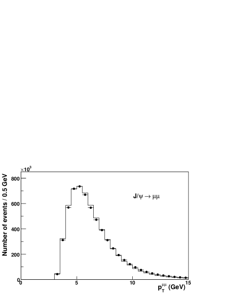
Figure 11: Distributions of $p_{T}^{\mu\mu}$ (top) and $\sum q/p_{T}^{\mu}$ (bottom) in the data (circles) and the tuned simulation of $J/\psi$ decays (histogram). The data distributions are background-subtracted using events in the mass range 3.17–3.31 GeV.

VII.2.3 Momentum scale measurement

The large size of the $J/\psi\to\mu\mu$ data sample allows for detailed corrections of nonuniformities in the magnetic field and alignment, and of mismodeling of the material in the silicon tracking detector. These corrections are determined by fitting for $\Delta p/p$, the relative momentum correction to each simulated muon, as a function of the mean $\cot\theta$ of the muons, the $\cot\theta$ difference between muons, or the mean inverse $p_{T}$ of the muons, respectively.

Nonuniformities in the magnetic field were determined prior to the tracking system installation and their effects are included in the trajectory reconstruction. Global COT misalignments can lead to additional nonuniformities, in particular at the longitudinal ends of the tracking detector. We measure the corresponding effect on the momentum scale using the mean $\cot\theta$ dependence of $\Delta p/p$ for the $J/\psi$ sub-sample with small longitudinal opening angle between the final-state muons, $|\Delta\cot\theta|<0.1$. Based on this dependence we apply the following correction to the measured track $p_{T}$ in data:

$$p_{T}^{cor}=(1-0.00019\cdot\cot\theta+0.00034\cdot{\cot^{2}\theta})p_{T}.$$ (18)

After applying this correction, the fitted $\Delta p/p$ shows no significant dependence on $\cot\theta$ (Fig. 12).

Figure 12: Measured $\Delta p/p$ as a function of the mean $\cot\theta$ of the muon pair from $J/\psi$ decay, after requiring $|\Delta\cot\theta|<0.1$ and including corrections.

We study COT misalignments by measuring $\Delta p/p$ as a function of the difference in $\cot\theta$ between the muons tracks from a $J/\psi$ decay. A $z$-scale factor different from unity, equivalent to a scale factor on $\cot\theta$, can be caused by a small deviation of the stereo angles from their nominal values; this would lead to a quadratic variation of $\Delta p/p$ with $\Delta\cot\theta$. A relative rotation of the east and west endplates of the COT would lead to a linear dependence of $\Delta p/p$ on $\Delta\cot\theta$. These effects are reduced with respective corrections on the track $\cot\theta$ and curvature $c$ of the form

$$\begin{split}\cot\theta&\rightarrow s_{z}\cot\theta;\\ c&\rightarrow c-t\cot\theta.\end{split}$$ (19)

For muons from $J/\psi$ decay the dependence on $\Delta\cot\theta$ is removed with a $z$-scale correction $s_{z}=1.001640\pm 0.000018$ and a twist correction $t=(1.320\pm 0.092)\times 10^{-7}$ cm^-1.

The modeling of energy loss of muons traversing the silicon tracking detector is probed by measuring $\Delta p/p$ as a function of $\langle 1/p_{T}^{\mu}\rangle$, the mean unsigned curvature of the two muons. A bias in the modeling of ionization energy loss appears as a linear dependence of this measurement CDF2 . After applying a scale factor of 1.043 to the simulated amount of ionizing material in the tracking detectors, a linear fit in the range $\langle 1/p_{T}^{\mu}\rangle=(0.1,0.475)$ GeV^-1 gives a slope consistent with zero (Fig. 13, top). Using the fit to extrapolate to zero mean curvature, we find $\Delta p/p=(-1.311\pm 0.004_{\rm stat}\pm 0.022_{\rm slope/material})\times 10^{-3}$.

Figure 13: Top: Fractional momentum correction $\Delta p/p$ as a function of the mean inverse transverse momentum of the muons from $J/\psi$ decay. Bottom: Representative $m_{\mu\mu}$ fit (histogram) to data (circles), here in the range $\langle 1/p_{T}^{\mu}\rangle=(0.2,0.225)$ GeV^-1. The fit region is indicated by arrows.

VII.2.4 Systematic uncertainties

Systematic uncertainties on the momentum-scale correction extracted from $J/\psi\to\mu\mu$ decays are listed in Table 3. The dominant uncertainty arises from the modeling of the rising portion of the $m_{\mu\mu}$ lineshape. Since we model final-state QED radiation with a leading-log Sudakov factor CDF2 ; sudakov , the modeling of this region is imperfect. We estimate the corresponding uncertainty by varying the factorization scale $Q$ in the Sudakov form factor to minimize the sum-$\chi^{2}$ of the $\langle 1/p_{T}^{\mu}\rangle$-binned $J/\psi$ mass fits (one of these fits is shown in the bottom of Fig. 13). The change in the fitted $\Delta p/p$ for this $Q$ value, compared to the nominal value of $Q=m_{J/\psi}$, is $0.080\times 10^{-3}$.

We determine the impact of the nonuniformity of the magnetic field by applying the magnetic field correction obtained from $J/\psi\to\mu\mu$ data to $W\to\mu\nu$ data. The resulting shift in $M_{W}$ is in the same direction as the shift in the $J/\psi$ momentum scale, resulting in a partial cancellation of the corresponding uncertainty. The residual shift in $M_{W}$ corresponds to a momentum correction shift of $0.064\times 10^{-3}$. The uncertainty on the magnetic field correction is estimated to be 50%, resulting in an uncertainty of $0.032\times 10^{-3}$ on $\Delta p/p$ for the $M_{W}$ fit.

Fixing the slope in the fit to $\Delta p/p$ as a function of $\langle 1/p_{T}^{\mu}\rangle$ gives a statistical uncertainty of $0.004\times 10^{-3}$ on the $\Delta p/p$ correction at zero curvature. Including the slope variation, the uncertainty is $0.022\times 10^{-3}$, which is the effective uncertainty due to the ionizing material correction.

We quantify the uncertainty due to COT hit-resolution modeling by varying the resolution scale factor (see Sec. IV.4) determined using the sum-$\chi^{2}$ of the highest momentum bins in the $\langle 1/p_{T}^{\mu}\rangle$-binned $J/\psi$ mass fits. Fitting for this factor in individual $\langle 1/p_{T}^{\mu}\rangle$ bins, we observe a maximum spread of 3%. Assuming a uniform distribution gives a $1\sigma$ variation of 1.7%, which corresponds to an uncertainty on $\Delta p/p$ of $0.020\times 10^{-3}$.

The background in each $J/\psi\to\mu\mu$ mass distribution is described by a linear fit to the regions on either side of the peak. Varying the slope and intercept by their uncertainties in the inclusive $J/\psi$ sample leads to a shift in $\Delta p/p$ of $0.011\times 10^{-3}$, which is taken as the uncertainty due to background modeling.

The alignment corrections in Eq. (19) are varied by their uncertainties to obtain an uncertainty on $\Delta p/p$ of $0.009\times 10^{-3}$. To study the impact of unmodeled effects (such as trigger efficiencies) near the muon $p_{T}$ threshold, we increase this threshold by 200 MeV. The shift affects $\Delta p/p$ by $0.004\times 10^{-3}$, which is taken as an associated uncertainty.

The sensitivity of $\Delta p/p$ to the modeling of resolution tails is studied by changing the fit range by $\pm 20\%$. The $0.004\times 10^{-3}$ change in $\Delta p/p$ is taken as an uncertainty. Templates are simulated in $0.004\times 10^{-3}$ steps of $\Delta p/p$; we take half the step size as a systematic uncertainty due to the resolution of the $\Delta p/p$ fit. Finally, the uncertainty on the world-average $J/\psi$ mass contributes $0.004\times 10^{-3}$ to the uncertainty on $\Delta p/p$.

Including all systematic uncertainties, the momentum scale correction estimated using $J/\psi\to\mu\mu$ data is

$$[\Delta p/p]_{J/\psi}=(-1.311\pm 0.092)\times 10^{-3}.$$ (20)

Table 3: Fractional uncertainties on the muon momentum scale determined from $J/\psi$ and $\Upsilon$ mass measurements without a beam constraint on the muon tracks. The last column shows the uncertainty for each source that is common to the $J/\psi$ and $\Upsilon$ results.

Source	$J/\psi$ ($\times 10^{-3}$)	$\Upsilon$ ($\times 10^{-3}$)	Common ($\times 10^{-3}$)
QED and energy-loss model	0.080	0.045	0.045
Magnetic field nonuniformities	0.032	0.034	0.032
Ionizing material correction	0.022	0.014	0.014
Resolution model	0.020	0.005	0.005
Background model	0.011	0.005	0.005
COT alignment corrections	0.009	0.018	0.009
Trigger efficiency	0.004	0.005	0.004
Fit range	0.004	0.005	0.004
$\Delta p/p$ step size	0.002	0.003	0
World-average mass value	0.004	0.027	0
Total systematic	0.092	0.068	0.058
Statistical	0.004	0.025	0
Total	0.092	0.072	0.058

VII.3 $\Upsilon\to\mu\mu$ calibration

With a mass of $M_{\Upsilon}=9460.30\pm 0.26$ MeV pdg , the $\Upsilon(1S)$ resonance provides an intermediate-mass calibration reference between the $J/\psi$ meson and the $Z$ boson. Unlike $J/\psi$ mesons, all $\Upsilon$ mesons are produced promptly, so the reconstructed muon tracks from their decays can be constrained to the transverse beam position to improve momentum resolution. This allows a test for beam-constraint bias in a larger calibration sample than the $Z$-boson data sample zeng .

The online selection for $\Upsilon$ candidates is the same at level 1 as for selecting $J/\psi$ candidates (see Sec. VII.2.1). At level 2 at least one CMUP muon with $p_{T}>3$ GeV is required. The level 3 selection increases this threshold to 4 GeV and the $p_{T}$ threshold of the other muon to 3 GeV. The muons must have opposite charge and a pair invariant mass between 8 and 12 GeV. In the offline selection the $p_{T}$ thresholds are increased by 200 MeV and the muons are required to have $|d_{0}|<0.3$ cm and a small $z_{0}$ difference ($|\Delta z_{0}|<3$ cm). The COT hit requirements are the same as those applied to tracks from $W$- and $Z$-boson decays (see Sec. VI.1).

As with the $J/\psi\to\mu\mu$-based calibration, we use pythia pythia to generate muon four-momenta from $\Upsilon(1S)\to\mu\mu$ decays. We tune the simulation by increasing the rapidity of the $\Upsilon$ by $\Delta\zeta_{\upsilon}=ky_{\Upsilon}$, where $k=0.1$ for half of the mesons and $k=0.6$ for the other half. With this tuning, the kinematic properties of the $\Upsilon$ and the final-state muons are well described, as shown in Fig. 14.

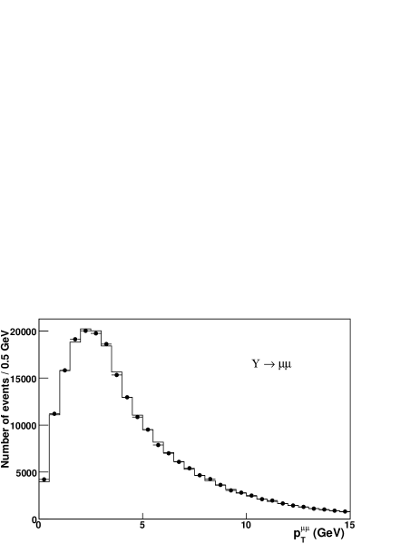
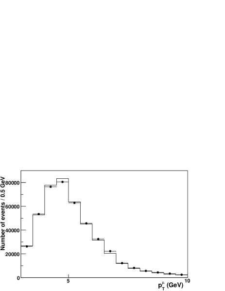
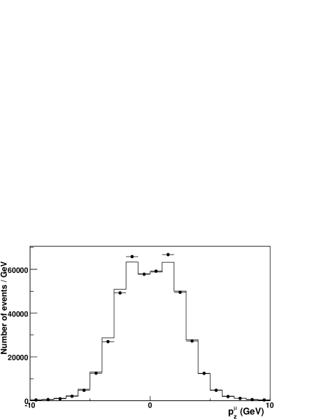
Figure 14: Distributions of $p_{T}^{\mu\mu}$ (top), $p_{T}^{\mu}$ (middle), and $p_{z}^{\mu}$ (bottom) in the data (circles) and the tuned simulation of $\Upsilon$ decays (histogram). The data distributions correspond to the mass range $9.30-9.56$ GeV and are background-subtracted using events in the mass ranges $9.17-9.3$ GeV and $9.56-9.69$ GeV.

The correction for magnetic field nonuniformity measured in $J/\psi$ data (see Sec. VII.2.3) is applied to the $\Upsilon$ data. By fitting for $\Delta p/p$ as a function of $\langle 1/p_{T}\rangle$, we find that the material scale value of 1.043 determined with $J/\psi$ data removes any dependence on $\langle 1/p_{T}\rangle$.

The intermediate momentum range of the muons from $\Upsilon$-meson decays can lead to different sensitivity to misalignments than muons from $J/\psi$-meson or $W$- or $Z$-boson decays. We measure the $z$-scale and twist corrections of Eq. (19) separately in $\Upsilon$ data, finding $s_{z}=1.00160\pm 0.00025$ ($1.00148\pm 0.00019$) and $t=0.50\pm 0.36~{}(2.10\pm 0.28)\times 10^{-7}$ cm^-1 for muon tracks without (with) a beam constraint.

In order to test for a beam-constraint bias, we fit for $\Delta p/p$ with and without incorporating the beam constraint. The fits are performed in the mass ranges $9.28<m_{\mu\mu}<9.58$ GeV and $9.245<m_{\mu\mu}<9.615$ GeV for the constrained and unconstrained tracks, respectively, and are shown in Fig. 15. The measurement with unconstrained tracks yields $\Delta p/p=(-1.335\pm 0.025_{\rm stat}\pm 0.068_{\rm syst})\times 10^{-3}$, where the systematic uncertainties are evaluated in a similar manner to the $J/\psi$-based calibration and are shown in Table 3. Using constrained tracks, the measurement yields $\Delta p/p=(-1.185\pm 0.020_{\rm stat}\pm 0.068_{\rm syst})\times 10^{-3}$. We correct the $\Upsilon$-based calibration with unconstrained tracks by half the difference between measurements obtained with unconstrained and constrained tracks, and take the correction ($\Delta p/p=0.075\times 10^{-3}$) as a systematic uncertainty on the calibration. The momentum scale correction estimated using $\Upsilon\to\mu\mu$ data is therefore

$$[\Delta p/p]_{\Upsilon}=(-1.260\pm 0.103)\times 10^{-3}.$$ (21)

Figure 15: Distribution of $m_{\mu\mu}$ for the best-fit templates (histograms) and the data (circles) in the $\Upsilon\to\mu\mu$ sample used to calibrate the muon momentum scale. The muon tracks are reconstructed with (top) or without (bottom) a constraint to the beam position in the transverse plane. The arrows enclose the fit region.

VII.4 Combination of $J/\psi$ and $\Upsilon$ calibrations

Table 4 summarizes the measured momentum scales from reconstructed samples of $J/\psi$ mesons, $\Upsilon$ mesons without a beam-constraint (NBC), and $\Upsilon$ mesons with a beam-constraint (BC). Since the $J/\psi$-based measurement is performed using tracks without a beam-constraint, we combine the results from $J/\psi$ and NBC $\Upsilon$ meson fits. Using the Best Linear Unbiased Estimator (BLUE) algorithm BLUE and accounting for the correlations listed in Table 3, we obtain

$$[\Delta p/p]_{J/\psi+NBC~{}\Upsilon}=(-1.329\pm 0.068)\times 10^{-3}.$$ (22)

As with the scale determination based on $\Upsilon$ meson decays only, we correct this result by half the difference with respect to the BC $\Upsilon$ meson result, and take the full correction as a systematic uncertainty. The final combined momentum scale based on measurements of $J/\psi$ and $\Upsilon$ mesons is

$$[\Delta p/p]_{J/\psi+\Upsilon}=(-1.257\pm 0.101)\times 10^{-3}.$$ (23)

Table 4: Summary of momentum scale determinations using $J/\psi$-meson data and $\Upsilon$-meson data with (BC) and without (NBC) beam-constrained tracks. The systematic uncertainties do not include the uncertainty stemming from the difference between the BC and NBC $\Upsilon$-meson results. The systematic uncertainties for the $\Upsilon$ samples are obtained using BC $\Upsilon$ data and assumed to be the same for NBC $\Upsilon$ data, since the sources are completely correlated.

Sample	$\Delta p/p(\times 10^{-3})$
$J/\psi\to\mu\mu$	$-1.311\pm 0.004_{\rm stat}\pm 0.092_{\rm syst}$
$\Upsilon\to\mu\mu$ (NBC)	$-1.335\pm 0.025_{\rm stat}\pm 0.068_{\rm syst}$
$\Upsilon\to\mu\mu$ (BC)	$-1.185\pm 0.020_{\rm stat}\pm 0.068_{\rm syst}$

VII.5 $Z\to\mu\mu$ mass measurement and calibration

Using the precise momentum scale calibration obtained from $J/\psi$ and $\Upsilon(1S)$ decays, we perform a measurement of the $Z$-boson mass in $Z\to\mu\mu$ decays. The measurement result was hidden during the calibration process, following the procedure described in Sec. II.3. After unblinding and testing the consistency of the measured $M_{Z}$ with the known value of $M_{Z}=91187.6\pm 2.1$ MeV pdg , we use the latter to further constrain $\Delta p/p$. The resulting calibration is then applied to the $W$-boson data for the $M_{W}$ measurement.

The $Z\to\mu\mu$ sample of 59 738 events is selected as described in Sec. VI.1 and includes the momentum scale calibration given in Eq. (23). We form templates for the $Z\to\mu\mu$ invariant mass lineshapes using the resbos generator, with final-state photon emission simulated using the photos generator and calibrated to the horace generator (Sec. V). We measure $M_{Z}$ using a binned likelihood template fit to the data in the range $83190<m_{\mu\mu}<99190$ MeV (Fig. 16). Systematic uncertainties on $M_{Z}$ are due to uncertainties on the COT momentum scale (9 MeV), alignment corrections (2 MeV), and QED radiative corrections (5 MeV). The alignment uncertainty is dominated by the uncertainty on the $z$-scale parameter $t$ of Eq. (19), as determined using BC $\Upsilon\rightarrow\mu\mu$ data.

The measurement of the $Z$-boson mass in the muon decay channel is

$$M_{Z}=91180\pm 12_{\rm stat}\pm 10_{\rm syst}~{}\textrm{MeV}.$$ (24)

This result is the most precise determination of $M_{Z}$ at a hadron collider and is in excellent agreement with the world-average value of $M_{Z}$, providing a sensitive consistency check of the momentum scale calibration. Combining this measurement with the calibration of Eq. (23) from $J/\psi$ and $\Upsilon$ data, and taking the alignment and QED uncertainties to be fully correlated, we obtain

$$[\Delta p/p]_{J/\psi+\Upsilon+Z}=(-1.29\pm 0.09)\times 10^{-3}.$$ (25)

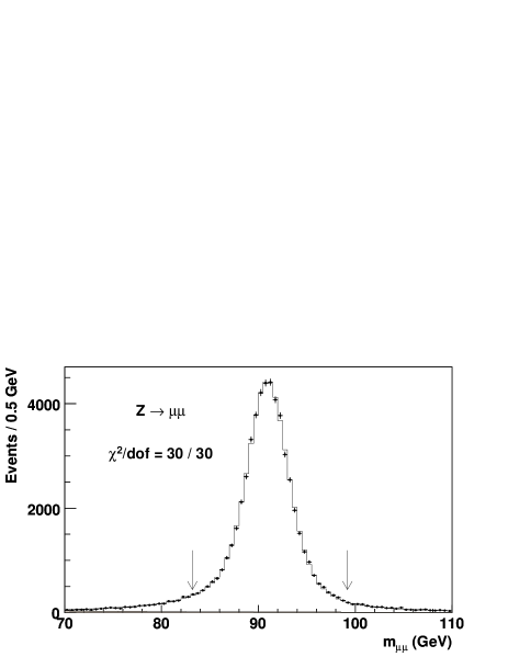
Figure 16: Distribution of $m_{\mu\mu}$ for the best-fit template (histogram) and data (circles) in the $Z\rightarrow\mu\mu$ candidate sample. The filled histogram shows the $\gamma^{*}\to\mu\mu$ contribution. The fit region is enclosed by the arrows.

VIII Electron Momentum Measurement

The mean fraction of traversed radiation lengths for an electron in the CDF tracking volume is approximately 19% CDF2 . Hence, electron track momentum measurements do not provide as high precision as calorimeter measurements. For the high-energy electrons used in this analysis, the bremsstrahlung photons are absorbed by the same calorimeter tower as the primary electron. We perform a precise calibration of the calorimeter response using the measured ratio of calorimeter energy to track momentum ($E/p$). We validate the calibration by measuring the mass of the $Z$ boson in $Z\to ee$ events and then combine the $E/p$ and $Z$-mass calibrations to obtain the calorimeter calibration used for the $M_{W}$ measurement.

VIII.1 $E/p$ calibration

The precise track momentum calibration is applied to calorimeter-based measurements through the ratio $E/p$. The calibration includes several corrections: the data are corrected for response variations near tower edges in $\phi$ and $z$ and the simulation is corrected for limitations in the knowledge of the number of radiation lengths in the tracking detector and the calorimeter, and for the observed energy dependence of the calorimeter response. Including in the model the energy resolution determined from the $E/p$ peak region and from $Z\to ee$ data (see Sec. IV.5), the calorimeter energy scale $S_{E}$ is extracted using a likelihood fit to the $E/p$ peak.

The dominant spatial nonuniformities in the CEM response are corrected in the event reconstruction cemresponse . Residual nonuniformities near gaps between towers are at the 1–2% level, as determined using the mean $E/p$ in the range 0.9–1.1. After correcting for these nonuniformities, the likelihood fits for the calorimeter energy scale are independent of electron $|\eta|$ (Fig. 17).

Figure 17: Measured calorimeter energy scale in bins of electron tower in $W\to e\nu$ data after corrections are applied. The towers are numbered in order of increasing $|\eta|$ and each tower subtends $\Delta\eta\approx 0.11$.

The radiative detector material is mapped into a three-dimensional lookup table, as described in Sec. IV. We fine-tune this material model with a likelihood fit to two ranges in the tail of the $E/p$ distribution ($1.1<E/p<1.6$), which is sensitive to the total number of radiation lengths traversed. The region $0.85<E/p<1.1$ effectively normalizes the simulation. From a maximum likelihood fit to electrons in $W\to e\nu$ ($Z\to ee$) data, we obtain a multiplicative factor $S^{W}_{\rm mat}=1.027\pm 0.004$ ($S^{Z}_{\rm mat}=1.001\pm 0.011$) to the number of radiation lengths in the simulation. The results from $W$ and $Z$ data are statistically consistent within $2.2\sigma$ and are combined to give the correction $S^{W,Z}_{\rm mat}=1.024\pm 0.003$ applied to the simulation for mass measurements. Figure 18 shows the three-bin $E/p$ distributions for both $W\to e\nu$ and $Z\to ee$ data after the correction factor is applied.

Figure 18: Distributions of $E/p$ in data (circles) and simulation with the best-fit value of $S^{W,Z}_{\rm mat}$ (histograms) in $W\rightarrow e\nu$ (top) and $Z\to ee$ (bottom) events.

Electron candidates with low $E/p$ are predominantly electron showers that are not fully contained in the EM calorimeter. Accurate simulation of these showers relies on a knowledge of the amount and composition of the CEM material. We tune the a priori estimate of this material using the relative fraction of electron candidates with low $E/p$ ($0.85<E/p<0.93$) to those at low $E/p$ or in the peak ($0.85<E/p<1.09$). From a comparison of data to simulation of this ratio as a function of the amount of tower material, we find that the data are accurately reproduced by adding a thin layer to each simulated calorimeter tower. The thickness of the additional tower increases linearly from zero for the central towers ($|\eta|\approx 0$) to $0.51X_{0}$ for the most forward tower ($|\eta|\approx 1$). The estimated uncertainty on the forward tower correction is $0.07X_{0}$.

We correct the energy dependence of the detector response by applying a per-particle scale in the simulation (Sec. IV.5). We measure this correction, $\xi$ in Eq. (8), using the fit energy scale as a function of measured calorimeter $E_{T}$ in $W\to e\nu$ and $Z\to ee$ data. Figure 19 shows the results of these fits after including the correction from the combined data, $\xi=(5.25\pm 0.70)\times 10^{-3}$.

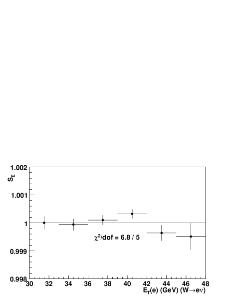
Figure 19: Measured energy scale as a function of electron $E_{T}$ for $W\to e\nu$ (top) and $Z\to ee$ (bottom) data. The simulation is corrected with the best-fit value of $\xi=(5.25\pm 0.70)\times 10^{-3}$.

After applying the complete set of corrections described above, we fit the peak region ($0.93<E/p<1.11$) of the $E/p$ distribution for $S_{E}$ in both $W\to e\nu$ and $Z\to ee$ data. The fits results are statistically consistent, differing by $(0.019\pm 0.030)\%$ between the two data sets; their combination has a statistical uncertainty of 0.008%. After applying the calibrated energy scale, the simulated $E/p$ distribution shows good agreement with the data for both $W\to e\nu$ and $Z\to ee$ events (Fig. 20).

By varying the simulation parameters we determine the correlations between the uncertainties on the energy scale estimated using $E/p$ and on $M_{W}$ obtained from the mass-fit distributions. The $E/p$-based calibration uncertainties on $M_{W}$ using the $m_{T}$ fit are due to $S_{\rm mat}$ (4 MeV), the tracker material model (3 MeV), calorimeter material (2 MeV), calorimeter nonlinearity (4 MeV), track momentum scale (7 MeV), and resolution (4 MeV). Including the statistical uncertainty gives a total $E/p$-based calibration uncertainty on $M_{W}$ of 12 MeV.

Figure 20: Distribution of $E/p$ for $W\to e\nu$ (top) and $Z\to ee$ (bottom) data (circles) after the full energy-scale calibration; the best-fit templates (histograms) are overlaid. The fit region is enclosed by arrows.

VIII.2 $Z\to ee$ mass measurement and calibration

As with the meson-based calibration of track momentum, the $E/p$-based calorimeter energy calibration is validated with a measurement of the $Z$-boson mass. After comparing the mass measured in $Z\to ee$ decays to the known value of $M_{Z}$, we incorporate the result into the electron energy calibration used for the $M_{W}$ measurement.

The $Z\to ee$ candidate sample contains 16 134 events. We use the same simulation and fit procedure as for the mass measurement using $Z\to\mu\mu$ decays, but with a broader fit range of $81\,190<m_{ee}<101\,190$ MeV (Fig. 21). We measure $M_{Z}=91\,230\pm 30_{\rm stat}$ MeV.

Figure 21: Best-fit $M_{Z}$ template (histogram) compared to data (circles) in $Z\to ee$ decays. The fit region is enclosed by arrows.

Systematic uncertainties on $M_{Z}$ are due to the $E/p$ calibration (10 MeV), the COT momentum-scale calibration (8 MeV), alignment corrections (2 MeV), and the QED radiative corrections (5 MeV). Including these uncertainties, the $Z$ boson mass determined using electron decays is

$$M_{Z}=91\,230\pm 30_{\rm stat}\pm 14_{\rm syst}~{}\textrm{MeV},$$ (26)

which is consistent with the known value of $M_{Z}$ at the level of $1.3\sigma$. The measurement is converted into an energy-scale calibration and combined with the $E/p$-based calibration to define the energy scale for the $M_{W}$ measurement. Taking into account correlations between uncertainties on the energy scale and on the fits for $M_{W}$, the uncertainty on $M_{W}$ due to the combined energy-scale calibration is 10 MeV.

The application of the momentum-scale calibration to a calorimeter energy calibration via $E/p$ relies on an accurate simulation of the electron radiation and the track reconstruction. We test the simulation by measuring $M_{Z}$ using electron track momenta only. The measurement is performed for three configurations: neither electron radiative (i.e., both with $E/p<1.1$), one electron radiative ($E/p>1.1$), and both electrons radiative. The results of the fits are shown in Table 5 and Fig. 22. Combining the measurements of events with at least one radiative electron gives $M_{Z}=91\,240\pm 38_{\rm stat}$ MeV, in good agreement with the known $M_{Z}$ and with the measurement determined using calorimeter energy. As an additional check, we split the calorimeter-based measurement into the same categories of radiative and nonradiative electrons, and obtain consistent results (Table 5 and Fig. 23).

Table 5: Summary of $M_{Z}$ measurements obtained using subsamples of data containing events with nonradiative electrons ($E/p<1.1$), one radiative electron ($E/p>1.1$), or two radiative electrons. Calorimeter-based and track-based measurements are shown for each category; uncertainties are statistical only.

Electrons	Calorimeter $M_{Z}$ (MeV)	Track $M_{Z}$ (MeV)
$E/p<1.1$ only	$91\,208\pm 39$	$91\,231\pm 41$
$E/p>1.1$ and $E/p<1.1$	$91\,234\pm 51$	$91\,294\pm 98$
$E/p>1.1$ only	$91\,370\pm 127$	$91\,176\pm 407$

Figure 22: Best-fit $M_{Z}$ templates (histogram) compared to data (circles) in $Z\to ee$ decays using only reconstructed track information in events with two nonradiative electrons (top), one radiative electron (middle), or two radiative electrons (bottom). The nonradiative fit region is enclosed by arrows; the other fit regions are to the left of the arrows.

Figure 23: Best-fit $M_{Z}$ templates (histogram) compared to data (circles) in $Z\to ee$ decays in events with two nonradiative electrons (top), one radiative electron (middle), and two radiative electrons (bottom). Fit regions are enclosed by arrows.

IX Recoil measurement

The neutrino transverse momentum is determined using a measurement of the recoil $\vec{u}_{T}$, defined in Eq. (2). To minimize bias in the recoil measurement, we correct the data to improve the uniformity of the calorimeter response. The recoil simulation models the removal of underlying event energy in the vicinity of each lepton, the response to QCD and QED initial-state radiation through a parametrization, the response to final-state photons using the same detailed accounting as for the lepton momentum calibration, and the response to the energy from the underlying event and additional $p\mathrm{bar}{p}$ collisions. The parameters are determined using events containing $Z$-boson decays to electrons or muons, since the dilepton transverse momentum is measured to high precision.

IX.1 Data corrections

The modeling of the recoil projected along the lepton direction directly impacts the $M_{W}$ measurement, as described in Sec. II.3. To simplify the modeling of the recoil direction, we apply corrections to the data to reduce nonuniformities in recoil response.

The uncorrected recoil has a sinusoidal distribution as a function of $\phi$, due in part to the offset of the collision point from the origin (in the radial direction). Calorimeter towers in the direction of the offset subtend a larger angle than those in the opposite direction, resulting in a higher energy measurement on average. A relative misalignment between the calorimeter and the beam has a similar effect, with an additional bias due to the mismeasured azimuthal angle of the tower. The azimuthal dependence increases with $|\eta|$ CDF2 , so the plug calorimeter towers have the largest dependence. For simplicity we remove the recoil variation by adjusting the origin of each plug calorimeter in our simulation. We use the minimum-bias data to parametrize these effective shifts in three time periods to correct for the sinking of the detector into the earth. Uniformity is improved by increasing the transverse energy threshold to 5 GeV for the two most forward towers in each plug detector, corresponding to the region $|\eta|>2.6$.

In addition to the azimuthal uniformity correction, we improve the recoil measurement resolution by applying a relative energy scale between the central and plug calorimeters CDF2 .

IX.2 Lepton tower removal

The measured recoil $\vec{u}_{T}$ in the data is determined by summing over the transverse momenta of all calorimeter towers with $|\eta|<2.6$, excluding towers with lepton energy deposits. The excluded towers are chosen by studying the average energy deposition in towers in the vicinity of the lepton. In the simulation we subtract an estimated underlying event energy in each event to model the lepton tower removal, with corrections for its dependence on $u_{||}$, $|u_{\perp}|$, and $|\eta|$.

We define the set of excluded calorimeter towers based on the presence of an average excess of energy over the uniform underlying event energy distribution. The ionization energy deposited by muons is highly localized, but spans neighboring towers in $\eta$ when a muon originates from a vertex with large $|z_{0}|$. We therefore remove the central tower, defined by the CES position of the muon, and both neighboring towers in $\eta$. The average energy in these and surrounding towers is shown in Fig. 24. The additional observed energy in the nearest tower in $\phi$ is due to final-state QED radiation, which is modeled by the simulation and is accurately described in this tower. Electrons shower across towers in both $\eta$ and $\phi$, and produce more QED final-state radiation. The number of removed electron towers is therefore larger, as shown in Fig. 25.

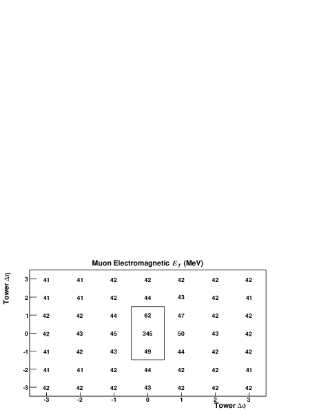
Figure 24: Average measured energy (in MeV) in the electromagnetic (top) and hadronic (bottom) calorimeters in the vicinity of the muon in $W$-boson decays. The differences $\Delta\phi$ and $\Delta\eta$ are signed such that positive differences correspond to towers closest to the muon position at the CES detector. The three towers inside the box are removed from the recoil measurement.

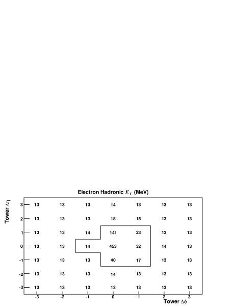
Figure 25: Average measured energy (in MeV) in the electromagnetic (top) and hadronic (bottom) calorimeters in the vicinity of the electron shower in $W$-boson decays. The differences $\Delta\phi$ and $\Delta\eta$ are signed such that positive differences correspond to towers closest to the electron shower position at the CES detector. The seven towers inside the box are removed from the recoil measurement.

To model the underlying event energy removed from the excluded towers, we use the energy distribution of equivalent towers separated by $90^{\circ}$ in $\phi$ from the lepton. The $90^{\circ}$ rotation is chosen to minimize bias from QED radiation and from kinematic selection, which depends primarily on $u_{||}$. Muon identification is emulated by requiring the local hadronic energy to be less than 4.2 GeV (the muon deposits 1.8 GeV of ionization energy on average in the hadronic calorimeter). The electron $E_{\rm had}/E_{\rm EM}$ and $L_{\mathrm{shr}}$ identification requirements are emulated by respectively requiring the local $E_{\rm had}$ to be less than 10% of the measured electron energy, and the neighboring tower in $\eta$ to have less than 5% of the electron energy.

In the simulation, we sample from the underlying event distribution measured in the rotated towers of all $W$-boson candidate events in the appropriate decay channel. We scale the extracted energy to account for the measured dependence on $u_{||}$, $|u_{\perp}|$, and $|\eta|$ (Figs. 26 and 27). The procedure is validated by applying the removal to a window rotated by $180^{\circ}$ from the lepton and comparing to data. The mean underlying event energy in this region is modeled to an accuracy of 1 MeV (2 MeV) in the muon (electron) channel. We take this as an estimate of the systematic uncertainty on the choice of rotation angle, and combine it with a parametrization uncertainty of 2 MeV for the electron channel and a selection bias uncertainty of 1 MeV for the muon channel. The total systematic uncertainty on $M_{W}$ due to lepton-removal modeling in the muon (electron) channel is 2 MeV (3 MeV), 2 MeV (3 MeV), and 4 MeV (6 MeV) for the $m_{T}$, $p_{T}^{\ell}$, $p_{T}^{\nu}$ fits, respectively.

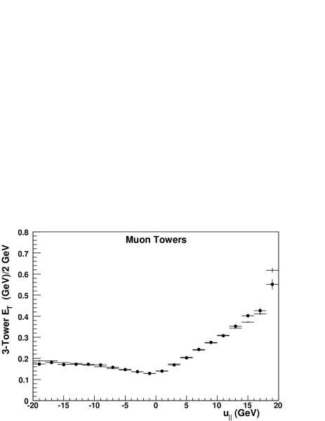
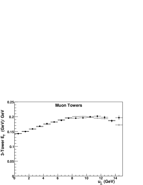
Figure 26: Variation of underlying event $E_{T}$ in the three-tower region rotated by $90^{\circ}$ in $\phi$ from the muon as a function of $u_{||}$ (top), $|u_{\perp}|$ (middle), and $\eta$ (bottom) for $W\to\mu\nu$ data (circles) and simulation (points).

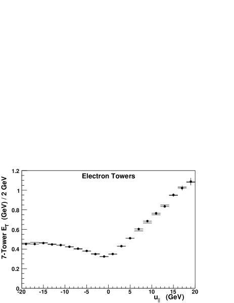
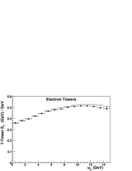
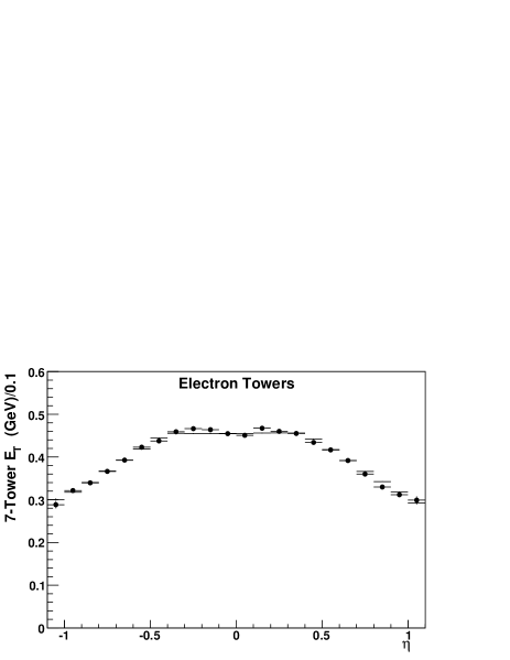
Figure 27: Variation of underlying event $E_{T}$ in the seven-tower region rotated by $90^{\circ}$ in $\phi$ from the electron as a function of $u_{||}$ (top), $|u_{\perp}|$ (middle), and $\eta$ (bottom) for $W\to e\nu$ data (circles) and simulation (points).

IX.3 Model parametrization

The recoil response model consists of a parametrization of three major sources: QCD and QED radiation in the parton-parton interaction producing a $W$ or $Z$ boson, radiation from the underlying event, and any additional $p\mathrm{bar}{p}$ collisions in the bunch crossing. The parameters are tuned using $Z\to\ell\ell$ events, since the lepton-pair $p_{T}$ is accurately measured and the balance between $p_{T}(Z\to\ell\ell)$ and $u_{T}$ probes the detector response and resolution. We define the axis parallel to $p_{T}(Z\to\ell\ell)$ as the “$\eta$” axis (Fig. 28) UA2etaxi , and the orthogonal axis in the transverse plane as the “$\xi$” axis.

Figure 28: Illustration of the $\eta$ and $\xi$ axes in $Z$ boson events.

IX.3.1 Recoil response

The response of the calorimeter to the radiation produced in the recoil of a $W$ or $Z$ boson is defined as the ratio of measured recoil to true recoil, projected along the direction of the true recoil ($R\equiv\vec{u}_{T}\cdot\hat{u}^{\mathrm{true}}/u_{T}^{\mathrm{true}}$, where $\vec{u}_{T}^{\mathrm{true}}=-\vec{p_{T}}^{W,Z}$ is the net $\vec{p}_{T}$ of the initial-state radiation). The simulation parametrizes the response function as

$$R=a\log(cu_{T}^{\mathrm{true}}+b)/\log(c\cdot 15~{}{\rm GeV}+b),$$ (27)

where $u_{T}^{\mathrm{true}}$ is expressed in units of GeV, and $a$, $b$, and $c$ are positive constants determined from $Z$-boson data. This functional form is empirically motivated by an approximation to $R$ measured in $Z$-boson data, $-\vec{u}_{T}\cdot\hat{p}_{T}^{\ell\ell}/p_{T}^{\ell\ell}$ (Fig. 29).

The parameters in Eq. (27) are determined using the balance between the recoil and dilepton momenta, $p_{\eta}^{\ell\ell}+u_{\eta}$, which is well defined when the boson is produced at rest. In the case of perfect response this sum would be zero; in practice the calorimeter response to the recoil is about 65% for the relevant $p_{T}$ range in this analysis. Figure 30 shows $0.65p_{\eta}^{\ell\ell}+u_{\eta}$ for the following best-fit values of $a$, $b$, and $c$:

$$\begin{split}a&=0.645\pm 0.002\\ b&=8.2\pm 2.2\\ c&=5.1\pm 0.6~{}{\rm GeV}^{-1},\end{split}$$ (28)

where the central values are obtained from minimizing the combined $\chi^{2}$ for electron and muon distributions, and the uncertainties are statistical. These values are used to model the recoil response in simulated $W$ and $Z$ boson events.

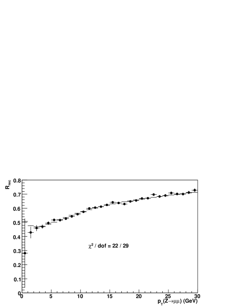
Figure 29: Mean value of $R_{\textrm{rec}}\equiv-\vec{u}_{T}\hat{p}_{T}^{~{}\mu\mu}/p_{T}^{\mu\mu}$, which approximates the recoil response $R$, as a function of dimuon $p_{T}$. The distribution motivates the logarithmic parametrization of the response. The simulation (lines) models the data (circles) accurately.

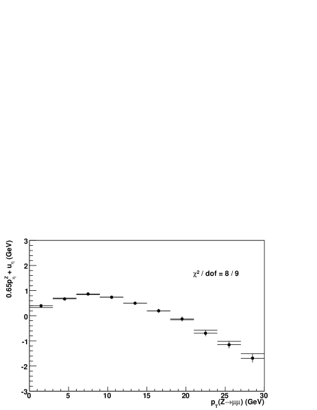
Figure 30: Distribution of $0.65p^{\ell\ell}_{\eta}+u_{\eta}$ for $Z$-boson decays to muons (top) and electrons (bottom) as a function of $Z$-boson $p_{T}$ in simulated (lines) and experimental (circles) data. The detector response parameters are obtained by minimizing the combined $\chi^{2}$ of these distributions.

IX.3.2 Recoil resolution

We parametrize the resolution on the recoil magnitude and direction using $Z\to\ell\ell$ data. The dominant effect is the sampling resolution

$$\sigma(u_{T})=s_{\mathrm{had}}\sqrt{u_{T}^{\mathrm{true}}},$$ (29)

where $s_{\mathrm{had}}$ is the calorimeter sampling constant. The rms resolution on the sum $0.65p_{\eta}^{\ell\ell}+u_{\eta}$ is used to fit for $s_{\mathrm{had}}$ in $Z\to\ell\ell$ data (Fig. 31, top), giving

$$s_{\mathrm{had}}=0.820\pm 0.009_{\rm stat}{\rm~{}GeV}^{1/2}.$$ (30)

Figure 31: Resolution on $0.65p^{\ell\ell}_{\eta}+u_{\eta}$ (left) and $0.65p^{\ell\ell}_{\xi}+u_{\xi}$ (right) in simulated (lines) and data (circles) $Z$-boson decays to muons (top) and electrons (bottom). The sum of the $\chi^{2}$ values in the $\xi$ or $\eta$ direction is minimized in the fit for the jet angular resolution parameters or the recoil resolution parameters ($N_{W,Z}$ and $s_{\mathrm{had}}$), respectively.

Figure 32: Distributions of the angular separation between the reconstructed recoil vector $\vec{u}_{T}$ and the dilepton $-\vec{p}_{T}^{\ell\ell}$ vector in $Z\rightarrow ee$ decays, for simulation (lines) and data (circles) respectively. The distributions are shown for the ranges $p_{T}^{\ell\ell}<8$ GeV (top), $8<p_{T}^{\ell\ell}<15$ GeV (middle), and $p_{T}^{\ell\ell}>15$ GeV (bottom).

The angular resolution $\sigma(u_{\phi})$ is modeled as a flat distribution with an rms parametrized as a continuous, piecewise-linear function separated into the ranges $0<u_{T}^{\mathrm{true}}<15$ GeV, $15<u_{T}^{\mathrm{true}}<30$ GeV and $u_{T}^{\mathrm{true}}>30$ GeV. This monotonically-improving resolution with increasing $u_{T}^{\mathrm{true}}$ is motivated by inspecting the angular separation between $\vec{u}_{T}$ and $-\vec{p}_{T}^{\ell\ell}$ in $Z\to\ell\ell$ decays. As illustrated in Fig. 32, the distribution of this angular separation, which is sensitive to $\sigma(u_{\phi})$, narrows with increasing $p_{T}^{\ell\ell}$. The parameters defining the $\sigma(u_{\phi})$ function are its values at $u^{\rm true}_{T}=9.4$ GeV, 15 GeV, and 24.5 GeV, respectively, chosen so that the parameter uncertainties are uncorrelated. We refer to these parameters as $\alpha$, $\beta$, and $\gamma$ respectively, such that

$$\sigma(u_{\phi})-\alpha ~{}~{}\propto 9.4-u^{\rm true}_{T}/{\rm GeV} (u^{\rm true}_{T}<15~{}{\rm GeV})$$

$$\sigma(u_{\phi}) ~{}~{}=\beta~{} (u^{\rm true}_{T}=15~{}{\rm GeV})$$

$$\sigma(u_{\phi})-\gamma ~{}~{}\propto 24.5-u^{\rm true}_{T}/{\rm GeV}~{} (15<u^{\rm true}_{T}<30~{}{\rm GeV})$$

$$\sigma(u_{\phi}) ~{}~{}={\rm constant}~{} (u^{\rm true}_{T}>30~{}{\rm GeV}),$$ (31)

where the unspecified coefficients are fixed by continuity. The parameters are tuned on the rms resolution of $0.65p_{\xi}^{\ell\ell}+u_{\xi}$ (Fig. 31, bottom), since the $\xi$-projection is much more sensitive to recoil angular fluctuations than to energy fluctuations. The fit using $Z\to\ell\ell$ data yields

$$\alpha = 0.306\pm 0.006_{\rm stat},$$

$$\beta = 0.190\pm 0.005_{\rm stat},$$

$$\gamma = 0.144\pm 0.004_{\rm stat}\;.$$ (32)

IX.3.3 Spectator and additional $p\mathrm{bar}{p}$ interactions

The resolution on the measured recoil receives contributions from energy produced by spectator partons and additional interactions CDF2 . We propagate these effects as a function of $\sum E_{T}$, the scalar sum of transverse energies in the calorimeter towers, in our simulation. For each simulated event, $\sum E_{T}$ is evaluated by adding two contributions sampled from distributions separately representing multiple interactions and spectator interactions accompanying the boson production. Given the $\sum E_{T}$ in an event, a corresponding contribution to the recoil ($\Delta u$) is calculated.

The $\sum E_{T}$ distributions are obtained from zero-bias and minimum-bias collision data for multiple interactions and spectator interactions, respectively. The zero-bias data are weighted to have an instantaneous luminosity profile consistent with that of the $W$ and $Z$ boson data. The minimum-bias distribution is scaled by a parameter $N_{V}$ to account for differences in spectator interactions in $W$ and $Z$ boson production relative to minimum-bias production. The parameter is measured using a combined $\chi^{2}$ fit for $N_{V}$ and $s_{\mathrm{had}}$ (Sec. IX.3.2) using the rms resolution on the sum $0.65p_{\eta}^{\ell\ell}+u_{\eta}$. The fit yields the result

$$N_{V}=1.079\pm 0.012_{\rm stat}.$$ (33)

The net contribution to the measured recoil is calculated from the total $\sum E_{T}$ in a simulated event as

$$\Delta u_{x,y}=A_{x,y}+B_{x,y}\sum E_{T}\oplus\sigma_{x,y}\left(\sum E_{T}\right),$$ (34)

where the parameters $A_{x,y}=(-11,23)$ MeV and $(B_{x},B_{y})=(0.00083,-0.00087)$ are obtained from a linear fit to the mean $\Delta u$ in minimum-bias data, and the resolution parameters are determined from power-law fits to the resolution on $\Delta u$ in minimum-bias data,

$$\sigma_{x,y}=0.3852\left(\sum E_{T}\right)^{0.5452}\textrm{ GeV}.$$ (35)

IX.4 Model tests

The recoil model, tuned from $Z$ boson events, is applied to simulated $W$ boson events. We validate the model by comparing the simulated $W$-boson recoil to the recoil measured in data. We utilize two projections of the recoil, along ($u_{||}$) and perpendicular to ($u_{\perp}$) the charged lepton momentum (Sec. II.2), as well as the total recoil $u_{T}$. Comparing the $u_{||}$ distributions in data and in simulation (Fig. 33) shows no evidence of a bias. We also compare the $u_{\perp}$ distribution (Fig. 34), which is dominantly affected by recoil resolution, in data and in simulation and find no evidence of a bias. The distribution of $u_{T}$ in both $W\to\mu\nu$ and $W\to e\nu$ data is well-modeled by our tuned simulation (Fig. 35). Consistency checks with $Z$ bosons decaying to forward ($|\eta|>1$) electrons show consistency of the relative central-to-plug calorimeter calibration malik .

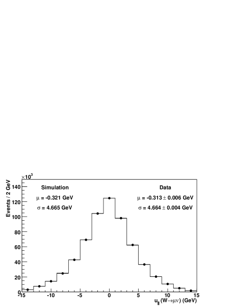
Figure 33: Distributions of $u_{||}$ from simulation (histogram) and data (circles) for $W$ boson decays to $\mu\nu$ (top) and $e\nu$ (bottom) final states. The simulation uses parameters fit from $Z$ boson data, and the uncertainty on the simulation is due to the statistical uncertainty on these parameters. The data mean ($\mu$) and rms spread ($\sigma$) are well-modeled by the simulation.

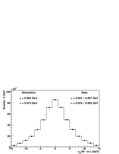
Figure 34: Distributions of $u_{\perp}$ from simulation (histogram) and data (circles) for $W$ boson decays to $\mu\nu$ (top) and $e\nu$ (bottom) final states. The simulation uses parameters fit from $Z$ boson data, and the uncertainty on the simulation is due to the statistical uncertainty on these parameters. The data mean ($\mu$) and rms spread ($\sigma$) are well-modeled by the simulation.

Figure 35: Distributions of $u_{T}$ from simulation (histogram) and data (circles) for $W$ boson decays to $\mu\nu$ (top) and $e\nu$ (bottom) final states. The simulation uses parameters fit from $Z$ boson data, and the uncertainty on the simulation is due to the statistical uncertainty on these parameters. The data mean ($\mu$) and rms spread ($\sigma$) are well-modeled by the simulation.

We estimate the uncertainties on the $M_{W}$ fits from the recoil model by varying each parameter in the model by $\pm 1\sigma$ and assuming linear parameter-dependent variations of the $M_{W}$ estimate (Table 6). The total uncertainty on $M_{W}$ due to the recoil model is 9 MeV, 8 MeV, and 11 MeV from the $m_{T}$, $p_{T}^{\ell}$, and $p_{T}^{\nu}$ fits, respectively. The uncertainties are entirely correlated for the electron and muon channels as the parameters are obtained from combined fits to $Z\to ee$ and $Z\to\mu\mu$ data.

Table 6: Signed shifts in the $M_{W}$ fits, in MeV, due to $1\sigma$ increases in recoil model parameters.

Parameter	$m_{T}(l\nu)$	$p_{T}(l)$	$p_{T}(\nu)$
$a$	$+2$	$+5$	$-1$
$b$	$+4$	$-2$	$+1$
$c$	$+3$	$+3$	$-1$
Response total	5	6	2
$s_{had}$	$+1$	$+2$	$0$
$N_{V}$	$+4$	$-2$	$-9$
$\alpha$	$-4$	$0$	$-6$
$\beta$	$0$	$+3$	$-1$
$\gamma$	$-2$	$-3$	$+1$
Resolution total	7	5	11

X Backgrounds

While the $W\to\mu\nu$ and $W\to e\nu$ event selections (Sec. VI) result in high-purity samples, several small sources of background persist and can affect the distributions used for $M_{W}$ fits. Both the $W\to\mu\nu$ and $W\to e\nu$ samples have backgrounds resulting from $Z/\gamma^{*}\to ll$, where one lepton is not detected; $W\to\tau\nu$ where the $\tau$ decay products include a reconstructed lepton; and multijet events where at least one jet is mis-reconstructed as a lepton. The $W\to\mu\nu$ sample also contains backgrounds from cosmic rays as well as from long lived hadrons decaying to $\mu\nu X$ final states.

X.1 $W\rightarrow\mu\nu$ Backgrounds

We model the $Z/\gamma^{*}\to\mu\mu$ background using events generated with pythia pythia and simulated with a full geant GEANT -based detector simulation. The $W\to\tau\nu$ background is estimated using the custom simulation and checked with the full geant simulation. We use control regions in the data to model the multijet, cosmic ray, and hadronic decay-in-flight backgrounds.

As the full geant-based CDF II detector simulation, or “CDFSim”, models global detector inefficiencies, it is more suitable for estimating background normalizations than our custom fast simulation is. However, CDFSim does not model the detector response to underlying event energies as accurately as our fast simulation. Therefore, we tune the calorimeter energies simulated in CDFSim based on the tunings described in Sec. IX. The uncertainty on this tuning is propagated to the $M_{W}$ measurement as an uncertainty in the background normalization and shapes estimated for $Z/\gamma^{*}\to\mu\mu$ decays.

The $Z/\gamma^{*}\to\mu\mu$ background is determined from the ratio of $Z/\gamma^{*}\to\mu\mu$ to $W\to\mu\nu$ acceptances determined from CDFSim, multiplied by the corresponding ratio of cross sections times branching ratios. In the standard model, the ratio $\mathcal{R}\equiv\sigma\mathcal{B}(W\to\mu\nu)/\sigma\mathcal{B}(Z\to\mu\mu)$ has been calculated to be $10.69\pm 0.08$ wzprd . In our estimation of the $Z\to\mu\mu$ background, we take an uncertainty of $\pm 0.13$, which includes an additional 1% uncertainty due to the uncertainty on the ratio of $W$ and $Z$ boson acceptances. From this value of $\mathcal{R}$ and our measured acceptances, we estimate the $Z/\gamma^{*}\to\mu\mu$ background in the $W\to\mu\nu$ candidate sample to be $(7.35\pm 0.09)\%$. The background due to $Z$ boson decays constitutes a larger portion of the $W\to\mu\nu$ candidate sample than of the $W\to e\nu$ sample due to the limited coverage of the muon detection system in $\eta.$

To estimate the $W\to\tau\nu$ background, we incorporate the $W\to\tau\nu$ kinematic distributions, radiative corrections, predicted $\mathcal{B}(\tau\to\mu\nu\mathrm{bar}{\nu}\nu)$, and $\tau\to\mu\nu\mathrm{bar}{\nu}\nu$ decay spectrum, including $\tau$ polarization, into the custom simulation. Then, we estimate the ratio of events from $W\to\tau\nu\to\mu\nu\mathrm{bar}{\nu}\nu$ to $W\to\mu\nu$ to be 0.963%, with negligible statistical uncertainty. We verify this prediction using CDFSim, adopting the same approach used to predict the $Z\to\mu\mu$ background, and obtain a ratio of $(0.957\pm 0.009)\%$, where the uncertainty is due to limited Monte Carlo sample size. The ratio $W\to\tau\nu\to\mu\nu\mathrm{bar}{\nu}\nu/W\to\mu\nu$ predicted by the custom simulation, 0.963%, normalized to the observed candidate sample including all backgrounds, corresponds to an estimate of $(0.880\pm 0.004)\%$ for the $W\to\tau\nu$ background contribution.

Multijet events where a jet mimics a muon track contribute background to the $W\to\mu\nu$ candidate sample. To estimate this background, we use an artificial neural network (NN) jetnet that differentiates prompt muons (from $W$ and $Z$ boson decay) and muon candidates that arise from jets. As input variables to the NN, we utilize the calorimeter energy and track momenta in an $\eta-\phi$ cone of size 0.4 surrounding the muon candidate. We then construct histograms of the NN discriminant for control samples of pure signal and pure background events. For our signal control sample, we select muons from $W\to\mu\nu$ generated with pythia and simulated with CDFSim. For our background control sample, we select events from the data that satisfy the $W\to\mu\nu$ selection criteria except with $p_{T}^{\nu}<10$ GeV and $u_{T}<45$ GeV. We combine these spectra such that the summed spectrum matches the discriminant spectrum for muons from $W\rightarrow\mu\nu$ data. In this fitting process, the background fraction is allowed to vary as a free parameter and is extracted via $\chi^{2}$ minimization. Using this method zeng , we estimate the fraction of the $W\to\mu\nu$ candidate sample resulting from hadronic jets to be $(0.035\pm 0.025)\%$.

Long lived hadrons, such as $K$ and $\pi$ mesons, decaying into muons before the hadrons reach the calorimeter can mimic $W\to\mu\nu$ events. This decay-in-flight (DIF) background enters our candidate sample when a low-momentum meson decaying to a muon results in the reconstruction of a single high-$p_{T}$ track with an abrupt change of curvature in it (i.e., a kinked pattern). As described in Sec. VI.1, DIF events are reduced by imposing a cut on the number of times the hit residuals change sides along a COT track as well as imposing restrictions on track impact parameter and reconstruction quality. To estimate the residual DIF background, we fit the track $\chi^{2}/$dof distribution of $W\to\mu\nu$ candidates in the data to a sum of signal and DIF background templates. We use data events passing the $W\to\mu\nu$ selection criteria except that large track impact parameters ($2<d_{0}<5$ mm) are required for the DIF-enriched background template and $Z\to\mu\mu$ events for the signal template. After correcting for the presence of real $W\to\mu\nu$ events in the background template, we estimate the DIF background to be $(0.24\pm 0.08)\%$ in the $W\to\mu\nu$ candidate sample.

High-energy muons from cosmic rays can mimic $W\rightarrow\mu\nu$ events when passing close to the beam line and reconstructed as a muon track on only one side of the COT. The cosmic-ray identification algorithm searches for unreconstructed tracks and removes cosmic rays with approximately 99% efficiency cosmic . The residual cosmic-ray background is estimated using the reconstructed interaction time $t_{0}$ and transverse impact-parameter magnitude $|d_{0}|$ from the COT track fit. We use the estimate for the cosmic-ray background from the smaller data set reported in Ref. CDF2 and scale it by the ratio of run-time to integrated luminosity to obtain the cosmic-ray background fraction in the $W\to\mu\nu$ candidate sample of $(0.02\pm 0.02)\%$.

Table 7: Background fractions from various sources in the $W\rightarrow\mu\nu$ data set, and the corresponding uncertainties on the $m_{T}$, $p_{T}^{\mu}$, and $p_{T}^{\nu}$ fits for $M_{W}$.

	Fraction of	$\delta M_{W}$ (MeV)
Source	$W\rightarrow\mu\nu$ data (%)	$m_{T}$ fit	$p_{T}^{\mu}$ fit	$p_{T}^{\nu}$ fit
$Z/\gamma^{*}\rightarrow\mu\mu$	$7.35\pm 0.09$	2.2	4.0	5.4
$W\rightarrow\tau\nu$	$0.880\pm 0.004$	0.2	0.2	0.2
Hadronic jets	$0.035\pm 0.025$	0.5	0.7	1.0
Decays in flight	$0.24\pm 0.08$	0.9	3.1	3
Cosmic rays	$0.02\pm 0.02$	0.5	1	0.7
Total	8.53 $\pm$ 0.12	3	5.2	5.7

The $m_{T}$, $p_{T}^{\mu}$, and $p_{T}^{\nu}$ distributions are obtained from the geant-based simulation for $W$ and $Z$ boson backgrounds, from identified cosmic ray events for the cosmic ray background, and from events in the $W\rightarrow\mu\nu$ sample with high-$\chi^{2}$ (isolation) muons for the decay-in-flight (hadronic jet) background. Including uncertainties on the shapes of the distributions, the total uncertainties on the background estimates result in uncertainties of 3, 5, and 6 MeV on $M_{W}$ from the $m_{T}$, $p_{T}^{\ell}$, and $p_{T}^{\nu}$ fits, respectively (Table 7).

X.2 $W\rightarrow e\nu$ Backgrounds

We model the $Z/\gamma^{*}\to ee$ background using pythia-generated events simulated with the geant-based CDFSim. We follow the same procedure used to estimate the $Z/\gamma^{*}\to\mu\mu$ background (Sec. X.1), correcting the reconstructed energies in CDFSim, and using the theoretical prediction of $R=10.69\pm 0.08$. We estimate the $Z/\gamma^{*}\to ee$ background in the $W\to e\nu$ candidate sample to be $(0.139\pm 0.014)\%$.

We model the $W\to\tau\nu$ background using our fast simulation, as with the $W\to\mu\nu$ channel. We estimate the ratio of events from $W\to\tau\nu\to e\nu\mathrm{bar}{\nu}\nu$ to $W\to e\nu$ to be 0.945%, which is consistent with the CDFSim prediction of $(0.943\pm 0.009_{\rm MC\;stat})$%. This ratio yields a prediction of the $W\to\tau\nu$ background in the $W\to e\nu$ candidate sample of $(0.93\pm 0.01)\%$.

As in the $W\to\mu\nu$ sample, multijet events enter the $W\to e\nu$ sample when a hadronic jet is misreconstructed as an electron. To estimate this background, we fit distributions of electron identification variables from $W\to e\nu$ candidate data to a sum of simulated electrons and background shapes. For the background sample, we select jet-enriched data events by applying the $W\to e\nu$ selection criteria (Sec. VI.2), except that the $m_{T}$ requirement is removed, $u_{T}$ is required not to exceed 45 GeV, and $p_{T}^{\nu}$ is required not to exceed 10 GeV. The identification variables are the weighted track isolation and the output of an artificial neural network (NN). The weighted track variable is the sum of the $p_{T}$ of particles within a $\eta-\phi$ cone of 0.4 and $\delta z_{0}=5$ cm around the identified electron’s track. The NN uses several kinematic variables used in $W\to e\nu$ selection, such as $E_{\rm had}/E_{\rm EM}$ and $\delta z$. As an alternative estimate, we fit the $p_{T}^{\nu}$ distribution of the $W\to e\nu$ candidate events to a sum of simulated $W\to e\nu$ events and jet-enriched events obtained using the NN. Using the results from all three fits, we obtain an estimate of the multijet background in the $W\to e\nu$ candidate sample of $(0.39\pm 0.14)\%$.

Table 8: Background fractions from various sources in the $W\rightarrow e\nu$ data set, and the corresponding uncertainties on the $m_{T}$, $p_{T}^{\mu}$, and $p_{T}^{\nu}$ fits for $M_{W}$.

	Fraction of	$\delta M_{W}$ (MeV)
Source	$W\rightarrow e\nu$ data (%)	$m_{T}$ fit	$p_{T}^{e}$ fit	$p_{T}^{\nu}$ fit
$Z/\gamma^{*}\to ee$	$0.139\pm 0.014$	1.0	2.0	0.5
$W\to\tau\nu$	$0.93\pm 0.01$	0.6	0.6	0.6
Hadronic jets	$0.39\pm 0.14$	3.9	1.9	4.3
Total	$1.46\pm 0.14$	4.0	2.8	4.4

The distributions for the $M_{W}$ fit variables are obtained from simulated events for $W$ and $Z$ boson backgrounds, and from events in the $W\rightarrow e\nu$ sample with low-NN electron candidates for the hadronic jet background. We fit these distributions and include their shapes and relative normalizations in the $M_{W}$ template fits. The uncertainties on the background estimates result in uncertainties of 4, 3, and 4 MeV on $M_{W}$ from the $m_{T}$, $p_{T}^{e}$, and $p_{T}^{\nu}$ fits, respectively (Table 8).

XI $W$-boson-mass fits

The $W$ boson mass is extracted by performing fits to a sum of background and simulated signal templates of the $m_{T}$, $p_{T}^{\ell}$, and $p_{T}^{\nu}$ distributions. The fits minimize $-\ln{\cal L}$, where the likelihood $\cal L$ is given by

$${\cal L}=\prod^{N}_{i=1}\frac{e^{-m_{i}}m_{i}^{n_{i}}}{n_{i}!},$$ (36)

where the product is over $N$ bins in the fit region with $n_{i}$ entries (from data) and $m_{i}$ expected entries (from the template) in the $i$th bin. The template is normalized to the data in the fit region. The likelihood is a function of $M_{W}$, where $M_{W}$ is defined by the relativistic Breit-Wigner mass distribution

$$\frac{d\sigma}{dm}\propto\frac{m^{2}}{(m^{2}-M_{W}^{2})^{2}+m^{4}\Gamma_{W}^{2}/M_{W}^{2}},$$ (37)

where $m$ is the invariant mass of the propagator. We assume the standard model $W$ boson width $\Gamma_{W}=2\,094\pm 2$ MeV. The uncertainty on $M_{W}$ resulting from $\delta\Gamma_{W}=2$ MeV is negligible.

XI.1 Fit Results

The $m_{T}$ fit is performed in the range $65<m_{T}<90$ GeV. Figure 36 shows the results of the $m_{T}$ fit for the $W\to\mu\nu$ and $W\to e\nu$ channels while a summary of the 68% confidence uncertainty associated with the fit is shown in Table 9. The $p_{T}^{\ell}$ and $p_{T}^{\nu}$ fits are performed in the ranges $32<p_{T}^{\ell}<48$ GeV and $32<p_{T}^{\nu}<48$ GeV, respectively, and are shown in Figs. 37 and 38, respectively. The uncertainties for the $p_{T}^{\ell}$ and $p_{T}^{\nu}$ fits are shown in Tables 10 and 11, respectively. The differences between data and simulation for the three fits, divided by the statistical uncertainties on the predictions, are shown in Figs. 39-41 and the fit results are summarized in Table 12.

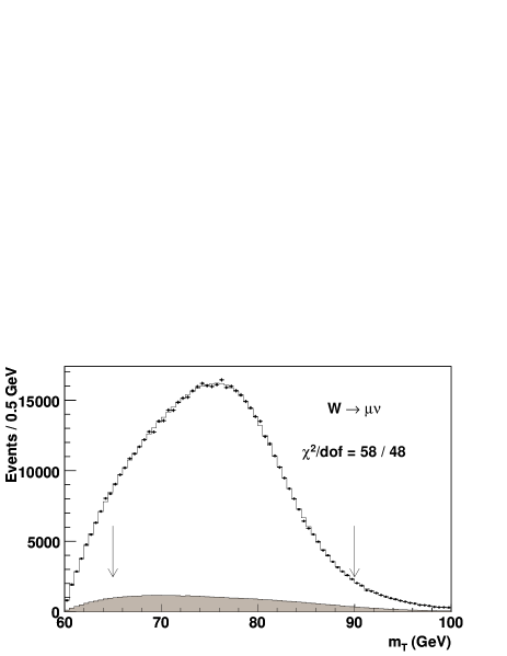
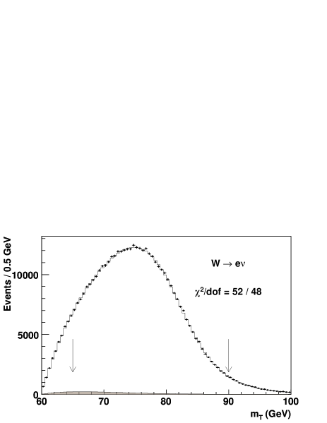
Figure 36: Distributions of $m_{T}$ for $W$ boson decays to $\mu\nu$ (top) and $e\nu$ (bottom) final states in simulated (histogram) and experimental (points) data. The simulation corresponds to the maximum-likelihood value of $M_{W}$ and includes backgrounds (shaded). The likelihood is computed using events between the two arrows.

Table 9: Uncertainties on $M_{W}$ (in MeV) as resulting from transverse-mass fits in the $W\to\mu\nu$ and $W\to e\nu$ samples. The last column reports the portion of the uncertainty that is common in the $\mu\nu$ and $e\nu$ results.

$m_{T}$ fit uncertainties
Source	$W\rightarrow\mu\nu$	$W\rightarrow e\nu$	Common
Lepton energy scale	7	10	5
Lepton energy resolution	1	4	0
Lepton efficiency	0	0	0
Lepton tower removal	2	3	2
Recoil scale	5	5	5
Recoil resolution	7	7	7
Backgrounds	3	4	0
PDFs	10	10	10
$W$ boson $p_{T}$	3	3	3
Photon radiation	4	4	4
Statistical	16	19	0
Total	23	26	15

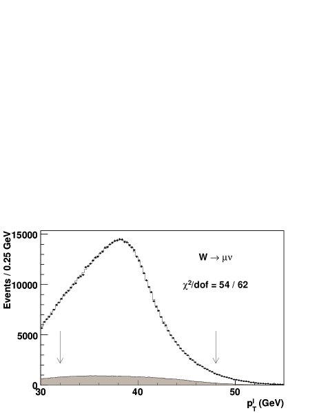
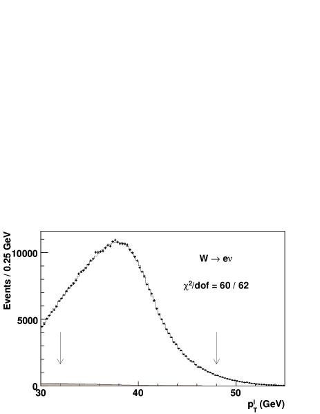
Figure 37: Distributions of $p_{T}^{\ell}$ for $W$ boson decays to $\mu\nu$ (top) and $e\nu$ (bottom) final states in simulated (histogram) and experimental (points) data. The simulation corresponds to the maximum-likelihood value of $M_{W}$ and includes backgrounds (shaded). The likelihood is computed using events between the two arrows.

Table 10: Uncertainties on $M_{W}$ (in MeV) as resulting from charged-lepton transverse-momentum fits in the $W\to\mu\nu$ and $W\to e\nu$ samples. The last column reports the portion of the uncertainty that is common in the $\mu\nu$ and $e\nu$ results.

$p_{T}^{\ell}$ fit uncertainties
Source	$W\rightarrow\mu\nu$	$W\rightarrow e\nu$	Common
Lepton energy scale	7	10	5
Lepton energy resolution	1	4	0
Lepton efficiency	1	2	0
Lepton tower removal	0	0	0
Recoil scale	6	6	6
Recoil resolution	5	5	5
Backgrounds	5	3	0
PDFs	9	9	9
$W$ boson $p_{T}$	9	9	9
Photon radiation	4	4	4
Statistical	18	21	0
Total	25	28	16

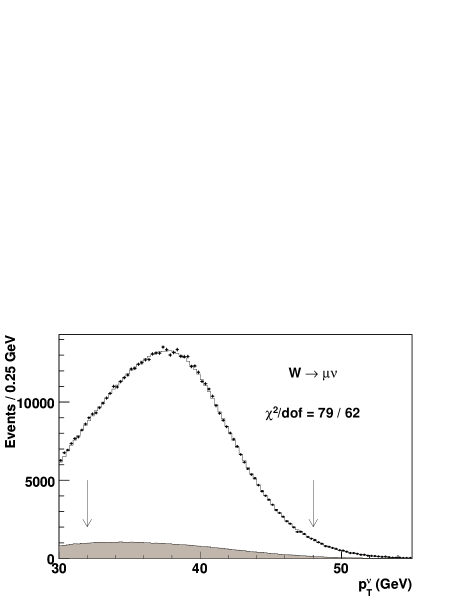
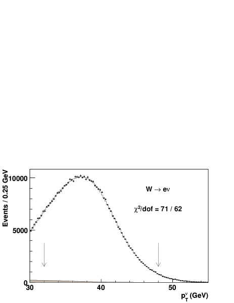
Figure 38: Distributions of $p_{T}^{\nu}$ for $W$ boson decays to $\mu\nu$ (top) and $e\nu$ (bottom) final states in simulated (histogram) and experimental (points) data. The simulation corresponds to the maximum-likelihood value of $M_{W}$ and includes backgrounds (shaded). The likelihood is computed using events between the two arrows.

Table 11: Uncertainties on $M_{W}$ (in MeV) as resulting from neutrino-transverse-momentum fits in the $W\to\mu\nu$ and $W\to e\nu$ samples. The last column reports the portion of uncertainty that is common in the $\mu\nu$ and $e\nu$ results.

$p_{T}^{\nu}$ fit uncertainties
Source	$W\rightarrow\mu\nu$	$W\rightarrow e\nu$	Correlation
Lepton energy scale	7	10	5
Lepton energy resolution	1	7	0
Lepton efficiency	2	3	0
Lepton tower removal	4	6	4
Recoil scale	2	2	2
Recoil resolution	11	11	11
Backgrounds	6	4	0
PDFs	11	11	11
$W$ boson $p_{T}$	4	4	4
Photon radiation	4	4	4
Statistical	22	25	0
Total	30	33	18

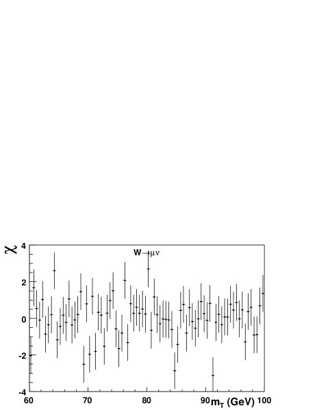
Figure 39: Differences between the data and simulation, divided by the expected statistical uncertainty, for the $m_{T}$ distributions in the muon (top) and electron (bottom) channels.

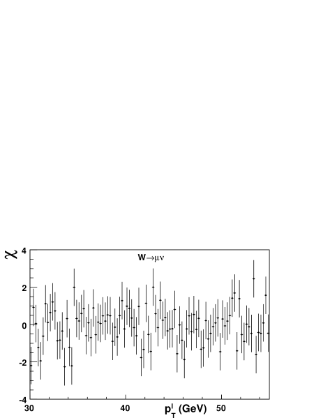
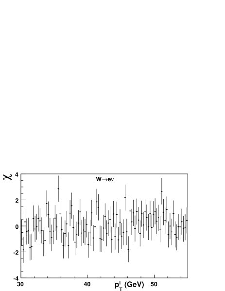
Figure 40: Differences between the data and simulation, divided by the expected statistical uncertainty, for the $p_{T}$ distributions in the muon (top) and electron (bottom) channels.

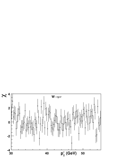
Figure 41: Differences between the data and simulation, divided by the expected statistical uncertainty, for the $p_{T}^{\nu}$ distributions in the muon (top) and electron (bottom) channels.

Table 12: Summary of fit results to the $m_{T}$, $p_{T}^{\ell}$, and $p_{T}^{\nu}$ distributions for the electron and muon decay channels.

Distribution	$M_{W}$ (MeV)	$\chi^{2}$/dof
$W\to e\nu$
$m_{T}$	$80\,408\pm 19$	52/48
$p_{T}^{\ell}$	$80\,393\pm 21$	60/62
$p_{T}^{\nu}$	$80\,431\pm 25$	71/62
$W\to\mu\nu$
$m_{T}$	$80\,379\pm 16$	57/48
$p_{T}^{\ell}$	$80\,348\pm 18$	58/62
$p_{T}^{\nu}$	$80\,406\pm 22$	82/62

Table 13: Statistical correlations between the $m_{T}$, $p_{T}^{\ell}$, and $p_{T}^{\nu}$ fits in the muon and electron decay channels.

Correlation	$W\rightarrow\mu\nu$ (%)	$W\rightarrow e\nu$ (%)
$m_{T}-p_{T}^{\ell}$	$67.2\pm 2.8$	$70.9\pm 2.5$
$m_{T}-p_{T}^{\nu}$	$65.8\pm 2.8$	$69.4\pm 2.6$
$p_{T}^{\ell}-p_{T}^{\nu}$	$25.5\pm 4.7$	$30.7\pm 4.5$

We utilize the best-linear-unbiased-estimator (BLUE) BLUE algorithm to combine individual fits. Each source of systematic uncertainty is assumed to be independent from all other sources of uncertainty within a given fit. We perform simulated experiments zeng to estimate the statistical correlation between fits to the $m_{T}$, $p_{T}^{\ell}$, and $p_{T}^{\nu}$ distributions (Table 13).

Combining the $M_{W}$ fits to the $m_{T}$ distributions in muon and electron channels, we obtain

$$M_{W}=80\,390\pm 20\textrm{ MeV}.$$ (38)

The $\chi^{2}$/dof for this combination is 1.2/1 and the probability that two measurements would have a $\chi^{2}/$dof at least as large is 28%.

Combining fits to the $p_{T}$ distributions in both muon and electron channels yields

$$M_{W}=80\,366\pm 22\textrm{ MeV}.$$ (39)

The $\chi^{2}$/dof for this combination is 2.3/1 with a 13% probability for the two measurements to result in $\chi^{2}/$dof $\geq 2.3$.

The result of combining the muon and electron channel fits to the $p_{T}^{\nu}$ distributions is

$$M_{W}=80\,416\pm 25\textrm{ MeV},$$ (40)

with a 49% probability of obtaining a $\chi^{2}/$dof value at least as large as the observed 0.5/1.

The combination of all three fits in the muon channel yields

$$M_{W}=80\,374\pm 22\textrm{ MeV},$$ (41)

with a $\chi^{2}$/dof of 4.0/2. Combining all three fits in the electron channel results in the value

$$M_{W}=80\,406\pm 25\textrm{ MeV},$$ (42)

with a $\chi^{2}$/dof of 1.4/2.

We combine all six fits to the final result,

$$M_{W}=80\,387\pm 19\textrm{ MeV}.$$ (43)

The relative weights, as calculated by the BLUE method BLUE , of the $m_{T}$, $p_{T}^{\ell}$, and $p_{T}^{\nu}$ fits in this combination are 53%, 31% and 16%, respectively. The contribution of the muon (electron) channel in the final combination is 62% (38%). The $\chi^{2}/$dof of this combination is 6.6/5 with a 25% probability of obtaining a $\chi^{2}/$dof at least as large. We evaluate the contribution from each source of systematic uncertainty in the combined measurement; these uncertainties are presented in Table 14.

Table 14: Uncertainties in units of MeV on the final combined result on $M_{W}$.

Source	Uncertainty
Lepton energy scale and resolution	7
Recoil energy scale and resolution	6
Lepton tower removal	2
Backgrounds	3
PDFs	10
$p_{T}(W)$ model	5
Photon radiation	4
Statistical	12
Total	19

XI.2 Consistency checks

We test our results for unaccounted systematic biases by dividing the data into several subsamples and comparing the electron and muon $p_{T}^{\ell}$ fit results obtained from these subsamples (Table 15). The uncertainty shown for $M_{W}$($\ell^{+}$)$-M_{W}$($\ell^{-}$) in the muon channel includes the systematic uncertainty on the mass fits in the $W^{+}\to\mu^{+}\nu$ and $W^{-}\to\mu^{-}\nu$ channels due to the COT alignment parameters $A$ and $C$ (Sec. VII.1), which contribute to this mass splitting. For the electron channel, we show the mass fit differences with and without applying an $E/p$-based calibration from the corresponding subsample. A residual dependence of the CEM energy scale on azimuth and time is observed. By suppressing this dependence through a calibration, the remaining variation of the electron channel mass fit is eliminated.

Table 15: Charged-lepton $p_{T}$-fit mass shifts (in MeV) for subdivisions of our data. For the spatial and time dependence of the electron channel fit result, we show the dependence without (with) the corresponding cluster energy calibration using the subsample $E/p$ fit. The variation observed without cluster energy recalibration is eliminated upon recalibration, proving that the effect arises dominantly due to residual variation of the energy scale.

Fit difference	$W\rightarrow\mu\nu$	$W\rightarrow e\nu$
$M_{W}$($\ell^{+}$)$-M_{W}$($\ell^{-}$)	$71\pm 70$	$-49\pm 42$
$M_{W}$($\phi_{\ell}>0$)$-M_{W}$($\phi_{\ell}<0$)	$-54\pm 36$	$-117\pm 42(-58\pm 45)$
$M_{W}$(Aug 2006-Sep 2007) $-$
$M_{W}$(Mar 2002-Aug 2006)	$116\pm 36$	$-266\pm 43(39\pm 45)$

The variations of the fitted mass values relative to the nominal results, as the fit regions are varied, are consistent with statistical fluctuations, as shown in Figs. 42-44 zeng . Furthermore, this consistency check is conservative, as the known systematic uncertainties are not included in displayed error bars. The systematic uncertainties that we consider (Tables 9-11) would induce additional expected shifts between shift regions. The observed shifts in Figs. 42-44 are typically substantially smaller than these systematic unertainties.

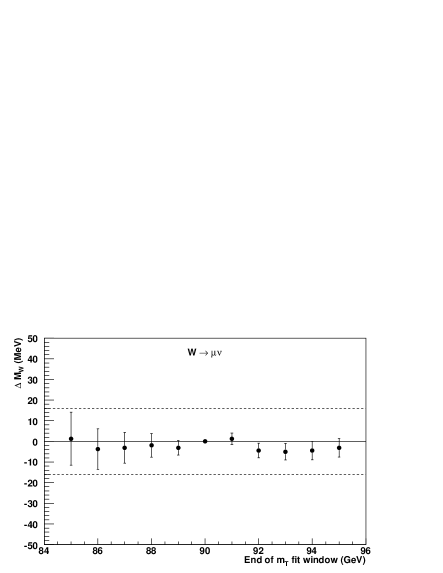
Figure 42: Variations of the $M_{W}$ value determined from the transverse-mass fit as a function of the choice of the (top) lower and (bottom) upper edge of the fit range, for the electron (left) and muon (right) channels. Uncertainty bars indicate expected variationwith respect to the default fit window, as computed using pseudoexperiments. The dashed lines indicate the statistical uncertainty from the default mass fit.

Figure 43: Variations of the $M_{W}$ value determined from the charged-lepton transverse-momentum fit as a function of the choice of the (top) lower and (bottom) upper edge of the fit range, for the electron (left) and muon (right) channels. Uncertainty bars indicate expected variation with respect to the default fit window, as computed using pseudoexperiments. The dashed lines indicate the statistical uncertainty from the default mass fit.

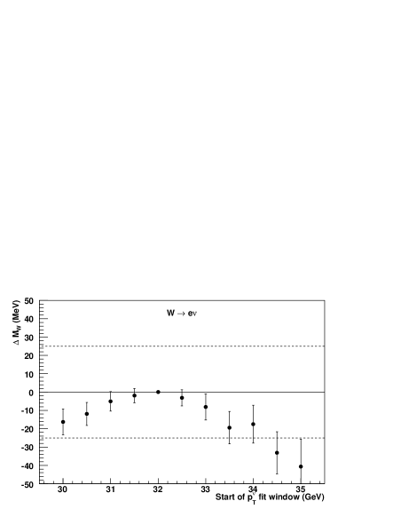
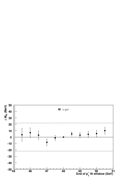
Figure 44: Variations of the $M_{W}$ value determined from the neutrino-transverse-momentum fit as a function of the choice of the (top) lower and (bottom) upper edge of the fit range, for the electron (left) and muon (right) channels. Uncertainty bars indicate expected variation with respect to the default fit window, as computed using pseudoexperiments. The dashed lines indicate the statistical uncertainty from the default mass fit.

XII Summary

We measure the $W$-boson mass using a sample of proton-antiproton collision data corresponding to an integrated luminosity of $2.2$ fb^-1 collected by the CDF II detector at $\sqrt{s}=1.96$ TeV. We use fits to $m_{T}$, $p_{T}$, and ${\hbox{$p$\kern-3.50006pt\lower-0.43057pt\hbox{/}}}_{T}\>$distributions of the $W\rightarrow\mu\nu$ and $W\rightarrow e\nu$ data samples to obtain

$$M_{W}=80387\pm 12_{\rm stat}\pm 15_{\rm syst}~{}{\rm MeV}=80387\pm 19~{}{\rm MeV},$$

which is the single most precise measurement of $M_{W}$ to date. This measurement subsumes the previous CDF measurement from a 200 pb^-1 subset of the present data CDF2 .

Using the method described in Ref. run2combo , we obtain a combined Tevatron result of

$$M_{W}=80385\pm 16~{}{\rm MeV.}$$

which includes the most recent measurement of $M_{W}$ from D0 dzero5fbprl .

Assuming no correlation between the Tevatron and LEP measurements, we obtain a new world average of

$$M_{W}=80385\pm 15~{}{\rm MeV.}$$

Following the discovery of the Higgs boson at the LHC and the measurement of its mass lhchiggs , all of the SM parameters required to make a prediction of the $W$-boson mass are now known. Including the radiative corrections mentioned in Eq. (1), the mass of the $W$ boson is predicted to be gfitter

$$M_{W}=80359\pm 11~{}{\rm MeV.}$$

The comparison of this prediction with our measurement over-constrains the SM and provides a stringent test of the radiative corrections. The level of consistency between the prediction and the measurement places bounds on non-SM physics that can affect $M_{W}$ at tree-level or via loops.

We thank the Fermilab staff and the technical staffs of the participating institutions for their vital contributions. This work was supported by the U.S. Department of Energy and National Science Foundation; the Italian Istituto Nazionale di Fisica Nucleare; the Ministry of Education, Culture, Sports, Science and Technology of Japan; the Natural Sciences and Engineering Research Council of Canada; the National Science Council of the Republic of China; the Swiss National Science Foundation; the A.P. Sloan Foundation; the Bundesministerium für Bildung und Forschung, Germany; the Korean World Class University Program, the National Research Foundation of Korea; the Science and Technology Facilities Council and the Royal Society, United Kingdom; the Russian Foundation for Basic Research; the Ministerio de Ciencia e Innovación, and Programa Consolider-Ingenio 2010, Spain; the Slovak R&D Agency; the Academy of Finland; the Australian Research Council (ARC); and the EU community Marie Curie Fellowship Contract No. 302103.

References

- (1) S. Glashow, Nucl. Phys. 22, 579 (1961); A. Salam and J. C. Ward, Phys. Lett. 13, 168 (1964); S. Weinberg, Phys. Rev. Lett. 19, 1264 (1967).
- (2) P. W. Anderson, Phys. Rev. 130, 439 (1960); F. Englert and R. Brout, Phys. Rev. Lett. 13, 321 (1964); P. W. Higgs, Phys. Rev. Lett. 13, 508 (1964); G. S. Guralnik, C. R. Hagen, and T. W. B. Kibble, Phys. Rev. Lett. 13, 585 (1964).
- (3) A. Sirlin, Phys. Rev. D 22, 971 (1980).
- (4) K. Nakamura et al. (Particle Data Group), J. Phys. G 37, 075021 (2010).
- (5) M. Ciuchini, E. Franco, S. Mishima, and L. Silvestrini, J. High Energy Phys. 08 (2013) 106; M. Baak, M. Goebel, J. Haller, A. Hoecker, D. Kennedy, K. Mönig, M. Schott, and J. Stelzer (The Gfitter Group), Eur. Phys. J. C 72, 2003 (2012).
- (6) G. Arnison et al. (UA1 Collaboration), Phys. Lett. B 122, 103 (1983); M. Banner et al. (UA2 Collaboration), Phys. Lett. B 122, 476 (1983); G. Arnison et al. (UA1 Collaboration), Phys. Lett. B 126, 398 (1983); P. Bagnaia et al. (UA2 Collaboration), Phys. Lett. B 129, 130 (1983).
- (7) T. Affolder et al. (CDF Collaboration), Phys. Rev. D 64, 052001 (2001).
- (8) V. M. Abazov et al. (D0 Collaboration), Phys. Rev. D 66, 012001 (2002); B. Abbott et al. (D0 Collaboration), Phys. Rev. D 62, 092006 (2000); B. Abbott et al. (D0 Collaboration), Phys. Rev. D 58, 092003 (1998).
- (9) S. Schael et al. (ALEPH Collaboration), Eur. Phys. Jour. C 47, 309 (2006).
- (10) J. Abdallah et al. (DELPHI Collaboration), Eur. Phys. Jour. C 55, 1 (2008).
- (11) P. Achard et al. (L3 Collaboration), Eur. Phys. Jour. C 45, 569 (2006).
- (12) G. Abbiendi et al. (OPAL Collaboration), Eur. Phys. Jour. C 45, 307 (2006).
- (13) T. Aaltonen et al. (CDF Collaboration), Phys. Rev. Lett. 99, 151801 (2007); T. Aaltonen et al. (CDF Collaboration), Phys. Rev. D 77, 112001 (2008).
- (14) V. M. Abazov et al. (D0 Collaboration), Phys. Rev. Lett. 103, 141801 (2009).
- (15) ALEPH, CDF, D0, DELPHI, L3, OPAL, and SLD Collaborations, the LEP Electroweak Working Group, the Tevatron Electroweak Working Group, and the SLD Electroweak and Heavy Flavour Groups, CERN Report No. CERN-PH-EP-2010-095, and Fermilab Report No. FERMILAB-TM-2480-PPD, 2010
- (16) T. Aaltonen et al. (CDF Collaboration), Phys. Rev. Lett. 108, 151803 (2012).
- (17) V. M. Abazov et al. (D0 Collaboration), Phys. Rev. Lett. 108, 151804 (2012).
- (18) T. Aaltonen et al. (CDF and D0 Collaborations), Phys. Rev. D 88, 052018 (2013).
- (19) J. Smith, W. L. van Neerven, and J. A. M. Vermaseren, Phys. Rev. Lett. 50, 1738 (1983).
- (20) F. Landry, R. Brock, P.M. Nadolsky, and C.-P. Yuan, Phys. Rev. D 67, 073016 (2003); C. Balazs and C.-P. Yuan, Phys. Rev. D 56, 5558 (1997); G.A. Ladinsky and C.-P. Yuan, Phys. Rev. D 50, 4239 (1994).
- (21) A. Abulencia et al. (CDF Collaboration), J. Phys. G 34 2457 (2007).
- (22) D. Acosta et al. (CDF Collaboration), Phys. Rev. D 71, 032001 (2005).
- (23) A. Sill et al., Nucl. Instrum. Methods Phys. Res., Sect. A 447, 1 (2000).
- (24) T. Affolder et al., Nucl. Instrum. Methods Phys. Res., Sect. A 526, 249 (2004).
- (25) D. Acosta et al., Nucl. Instrum. Methods Phys. Res., Sect. A 518, 605 (2004).
- (26) L. Balka et al., Nucl. Instrum. Methods Phys. Res., Sect. A 267, 272 (1988).
- (27) K. Yasuoka, S. Mikamo, T. Kamon, and A. Yamashita, Nucl. Instrum. Meth. Phys. Res., Sect. A 267, 315 (1987).
- (28) S. Bertolucci et al., Nucl. Instrum. Methods Phys. Res., Sect. A 267, 301 (1988).
- (29) H. Minemura et al., Nucl. Instrum. Methods Phys. Res., Sect. A 238, 18 (1985).
- (30) M. Albrow et al., Nucl. Instrum. Methods Phys. Res., Sect. A 480, 524 (2002); G. Apollinari et al., Nucl. Instrum. Methods Phys. Res., Sect. A 412, 515 (1998).
- (31) G. Ascoli et al., Nucl. Instrum. Methods Phys. Res., Sect. A 268, 33 (1988).
- (32) E. J. Thomson et al., IEEE Trans. Nucl. Sc. 49, 1063 (2002).
- (33) J. Elias et al., Nucl. Instr. Methods Phys. Res., Sect. A 441, 366 (2000).
- (34) R. Brun and F. Carminati, CERN Program Library Long Writeup, W5013, 1993 (unpublished), version 3.15.
- (35) E. Gerchtein and M. Paulini, arXiv:physics/0306031.
- (36) H. Bichsel, Rev. Mod. Phys. 60, 663 (1988).
- (37) G. R. Lynch and O. I. Dahl, Nucl. Instrum. Methods Phys. Res., Sect. B 58, 6 (1991).
- (38) Y.-S. Tsai, Rev. Mod. Phys. 46, 815 (1974).
- (39) D. Attwood et al. (MuScat Collaboration), Nucl. Instrum. Methods Phys. Res., Sect. B 251, 41 (2006).
- (40) T. Riddick, Ph.D. Thesis, University College London (2012), FERMILAB-THESIS-2012-57.
- (41) A. B. Migdal, Phys. Rev 103, 1811 (1956); L. D. Landau and I. J. Pomeranchuk, Dokl. Akad. Nauk. SSSR 92, 535 (1953); 92, 735 (1953).
- (42) M. L. Ter-Mikaelian, Dokl. Akad. Nauk. SSSR 94, 1033 (1954).
- (43) J. H. Hubbell, H. A. Gimm, and I. Ø verbø , J. Phys. Chem. Ref. Data 9, 1023 (1980).
- (44) M. Chen and P. Zerwas, Phys. Rev. D 12, 187 (1975).
- (45) A. V. Kotwal and C. Hays, Nucl. Intrum. Methods Phys. Res., Sect. A 729, 25 (2013).
- (46) P. Nadolsky, H. Lai, Q. Cao, J. Huston, J. Pumplin, D. Stump, W. Tung, and C.-P. Yuan, Phys. Rev. D 78, 013004 (2008); J. Pumplin, D.Stump, J. Huston, H. Lai, P. Nadolsky, and W. Tung, J. High Energy Phys. 0207, 012 (2002).
- (47) P. Golonka and Z. Was, Eur. Phys. J. C 45, 97 (2006).
- (48) C. M. Carloni Calame, G. Montagna, O. Nicrosini, and A. Vicini, J. High Energy Phys. 10 (2007) 109.
- (49) A. D. Martin, W. J. Sirling, R. S. Thorne, and G. Watt, Eur. Phys. Jour. C 63, 189 (2009).
- (50) D. Beecher, Ph.D. thesis, University College London (2011), FERMILAB-THESIS-2011-18.
- (51) Y. Zeng, Ph.D. thesis, Duke University (2012), FERMILAB-THESIS-2012-27.
- (52) J. C. Collins, D. Soper, and G. Sterman, Nucl. Phys. B250, 199 (1985).
- (53) Since the best-fit value of depends on the values of other parameters and PDFs used in the fitting model, we do not quote a measurement of . As a consistency check, we compare our best-fit value of GeV with the global-fit value of , and we find consistency considering that different PDFs yield an uncertainty on of .
- (54) W. T. Giele, E. W. N. Glover, and D. A. Kosower, Nucl. Phys. B403, 633 (1993).
- (55) J. C. Collins and D. E. Soper, Phys. Rev. D 16, 2219 (1977).
- (56) U. Baur, S. Keller, and D. Wackeroth, Phys. Rev. D 59, 013002 (1998).
- (57) A. V. Kotwal, H. K. Gerberich and C. Hays, Nucl. Instrum. Methods Phys. Res., Sect. A 506, 110 (2003).
- (58) F. Abe et al. (CDF Collaboration), Phys. Rev. D 52, 2624 (1995).
- (59) T. Sjstrand, Comput. Phys. Commun. 82, 74 (1994). We use version 6.129 for and production, version 6.136 for production, and version 6.157 for production.
- (60) V. V. Sudakov, Sov. Phys. JETP 3, 65 (1956).
- (61) L. Lyons, D. Gibaut, and P. Clifford, Nucl. Instrum. Methods Phys. Res., Sect. A 270, 110 (1988).
- (62) J. Alitti et al. (UA2 Collaboration), Phys. Lett. B 276, 354 (1992).
- (63) S. Malik, Ph.D. Thesis, University College London (2009), FERMILAB-THESIS-2009-59.
- (64) C. Peterson, T. Rgnvaldsson, and L. Lnnblad, Comput. Phys. Commun. 81, 185 (1994).
- (65) G. Aad et al. (ATLAS Collaboration), Phys. Lett. B 716, 1 (2012); S. Chatrchyan et al. (CMS Collaboration), Phys. Lett. B 716, 30 (2012).
- (66) M. Baak, M. Goebel, J. Haller, A. Hoecker, D. Kennedy, R. Kogler, K. Mönig, M. Schott, and J. Stelzer (GFitter Collaboration), Eur. Phys. J. C 72, 2205 (2012).