The Schramm–Loewner equation for multiple slits

Abstract

We prove that any disjoint union of finitely many simple curves in the upper half–plane can be generated in a unique way by the chordal multiple–slit Loewner equation with constant weights.

1 Introduction and results

Recent progress in the theory of Loewner equations ([Loe23, Sch00, Law05, BCD12]) suggests that one of the most useful descriptions of a simple plane curve is by encoding it into a growth process modeled by the Schramm–Loewner equation. In this paper we show that any disjoint union of finitely many simple curves can be encoded in a unique way into a growth process described by a multi–slit version of the Schramm–Loewner equation. In order to state our result we need to introduce some notation.

Let ${\mathbb{H}}:=\{z\in{\mathbb{C}}\ \vrule\ \mathop{{\rm Im}}(z)>0\}$ be the upper half–plane. A slit is the trace $\Gamma=\gamma(0,1]$ of a simple curve $\gamma:[0,1]\to\overline{{\mathbb{H}}}$ with $\gamma(0)\in{\mathbb{R}}$ and $\Gamma\subseteq{\mathbb{H}}$. Since ${\mathbb{H}}\backslash\Gamma$ is a simply connected domain, (a version of) Riemann’s mapping theorem guarantees that there is a unique conformal map $g_{\Gamma}$ from ${\mathbb{H}}\backslash\Gamma$ onto ${\mathbb{H}}$ with hydrodynamic normalization

$$g_{\Gamma}(z)=z+\frac{b}{z}+\mathcal{O}(|z|^{-2})\quad\text{ as }\quad z\to\infty\,$$

for some $b>0$. We call $\operatorname{hcap}(\Gamma):=b$ the half–plane capacity of the slit $\Gamma$. The following well–known result provides a description of the slit $\Gamma$ with the help of the chordal Loewner equation (Schramm–Loewner equation).

Theorem A (The one–slit chordal Loewner equation)

Let $\Gamma$ be a slit with $\operatorname{hcap}(\Gamma)=2T$. Then there exists a unique continuous driving function $U:[0,T]\to{\mathbb{R}}$ such that the solution $g_{t}$ to the chordal Loewner equation

$$\dot{g}_{t}(z)=\frac{2}{g_{t}(z)-U(t)},\quad g_{0}(z)=z,$$ (1.1)

has the property that $g_{T}=g_{\Gamma}$.

Note that in Theorem A the slit $\Gamma$ “starts” at the point $U(0)$.

To the best of our knowledge the first proof of Theorem A is due to Kufarev, Sobolev, Sporyševa in [KSS68]. The basic recent reference for Theorem A is the book of Lawler [Law05]. We also refer to the survey paper [GM13] for a complete and rigorous proof of Theorem A using classical complex analysis.

Now, let $\Gamma=(\Gamma_{1},\ldots,\Gamma_{n})$ be a multi–slit, that is, the union of $n$ slits $\Gamma_{1},\ldots,\Gamma_{n}$ with disjoint closures. As before, there is a unique conformal map $g_{\Gamma}$ from ${\mathbb{H}}\backslash\Gamma$ onto ${\mathbb{H}}$ with expansion

$$g_{\Gamma}(z)=z+b/z+\mathcal{O}(|z|^{-2})\quad\text{ as }\quad z\to\infty\,,$$

and we call $\operatorname{hcap}(\Gamma):=b>0$ the half–plane capacity of $\Gamma$. The main result of the present paper is the following extension of Theorem A.

Theorem 1.1

Let $\Gamma=(\Gamma_{1},\ldots,\Gamma_{n})$ be a multi–slit with $\operatorname{hcap}(\Gamma)=2T$. Then there exist unique weights $\lambda_{1},...,\lambda_{n}\in[0,1]$ with $\sum_{k=1}^{n}\lambda_{k}=1$ and unique continuous driving functions $U_{1},...,U_{n}:[0,T]\to{\mathbb{R}},$ such that the solution $g_{t}$ of the chordal Loewner equation

$$\dot{g}_{t}(z)=\sum_{k=1}^{n}\frac{2\lambda_{k}}{g_{t}(z)-U_{k}(t)},\qquad g_{0}(z)=z,$$ (1.2)

satisfies $g_{T}=g_{\Gamma}$.

Some remarks are in order.

Remark 1.2 (The multi–slit chordal Loewner equation)

It is well–known and easy to prove on the basis of Theorem A that under the conditions of Theorem 1.1 there are

• $n$ continuous weight functions $\lambda_{1},\ldots,\lambda_{n}:[0,T]\to{\mathbb{R}}$ with $\lambda_{j}(t)\geq 0$ and $\lambda_{1}(t)+\ldots+\lambda_{n}(t)=1$ for every $t\in[0,T]$, and

• $n$ continuous driving functions $U_{1},\ldots,U_{n}:[0,T]\to{\mathbb{R}}$,

such that the solution $g_{t}$ to the multi–slit chordal Loewner equation

$$\dot{g_{t}}(z)=\sum_{j=1}^{n}\frac{2\lambda_{j}(t)}{g_{t}(z)-U_{j}(t)},\quad g_{0}(z)=z\,,$$ (1.3)

satisfies $g_{T}=g_{\Gamma}$, see Remark 2.1 below. However, the $2n$ functions $\lambda_{j}(t)$ and $U_{j}(t)$ are not uniquely determined by the multi–slit $\Gamma$ if $n>1$, simply because in this case there are obviously many Loewner chains $\tilde{g}_{t}$ (in the sense of [Law05]) such that $\tilde{g}_{T}=g_{\Gamma}$. Informally, each weight function $\lambda_{j}(t)$ corresponds to the speed of growth of the slit $\gamma_{j}$ (the one that starts at the point $U_{j}(0)$). Theorem 1.1 shows that one can actually choose constant weight functions $\lambda_{j}$, which are moreover uniquely determined. In addition, then also the driving functions $U_{1}(t),\ldots,U_{n}(t)$ are uniquely determined by the multi–slit $\Gamma$. Hence Theorem 1.1 provides a canonical way of describing a multi–slit by a growth process modeled via a Loewner–type equation. We therefore call the differential equation (1.2), i.e., the multi–slit chordal Loewner equation with constant weights, the Schramm–Loewner equation for the multi–slit $\Gamma$.

Remark 1.3 (The multi–slit Loewner equation in Mathematical Physics)

We note in passing that the multiple–slit equation (1.3) has recently been used in mathematical physics for the study of certain two–dimensional growth phenomena. For instance, in [CM02] the authors analyze “Laplacian path models”, i.e. Laplacian growth models for multi–slits. By mapping the upper half–plane conformally onto a half-strip one obtains a Loewner equation for the growth of slits in a half–strip, which can be used to describe Laplacian growth in the “channel geometry”, see [GS08] and [DV11]. Furthermore, equation (1.3) can be used to model so–called multiple Schramm–Loewner evolutions, see [KL07] and [Car03], [BBK05], [Dub07], [Gra07].

Remark 1.4 (The multi–finger radial Loewner equation; Prokhorov’s theorem)

For the radial Loewner equation on the unit disk ${\mathbb{D}}:=\{z\in{\mathbb{C}}\ \vrule\ |z|<1\}$, the multi–slit situation has already been studied long time ago by Peschl [Pes36] in 1936. He proved that for every union $\Gamma$ of $n$ Jordan arcs $\Gamma_{1},\ldots,\Gamma_{n}$ in $\overline{{\mathbb{D}}}\backslash\{0\}$ such that ${\mathbb{D}}\backslash\Gamma$ is simply connected, there are continuous weight functions $\lambda_{1},\ldots,\lambda_{n}:[0,T]\to{\mathbb{R}}$ with $\lambda_{j}(t)\geq 0$ and $\lambda_{1}(t)+\ldots+\lambda_{n}(t)=1$ for every $t\in[0,T]$, and continuous driving functions $\kappa_{j}:[0,T]\to\partial{\mathbb{D}}$ such that the solution $w_{t}$ to the radial Loewner equation

$$\dot{w}_{t}(z)=-w_{t}(z)\sum\limits_{j=1}^{n}\lambda_{j}(t)\frac{\kappa_{j}(t)-w_{t}(z)}{\kappa_{j}(t)-w_{t}(z)}\,,\qquad w_{0}(z)=z\,,$$ (1.4)

has the property that $w_{T}$ maps ${\mathbb{D}}$ conformally onto ${\mathbb{D}}\backslash\Gamma$. As in the chordal case, this representation of the multi–slit $\Gamma$ is not unique. However, if the Jordan arcs $\Gamma_{1},\ldots,\Gamma_{n}$ are piecewise analytic, it is has been proved by D. Prokhorov [Pro93, Theorem 1 & 2] that one can choose constant weight functions and that then these weights as well as the continuous driving functions are uniquely determined. Prokhorov’s result forms the basis for his original and penetrating control–theoretic study of extremal problems for univalent functions, see his monograph [Pro93]. Clearly, Prokhorov’s result is the analogue of Theorem 1.1 for the radial Loewner equation (1.4), but only under the very restrictive additional assumption that the multi–slit is piecewise analytic. An extension of Prokhorov’s theorem for not necessarily piecewise analytic slits, i.e., the full analogue of Theorem 1.1 for the radial case will be discussed in the forthcoming paper [BS].

Remark 1.5 (Schramm–Loewner constants)

We call the constant weights $\lambda_{1},\ldots,\lambda_{n}$ in Theorem 1.1 the Schramm–Loewner constants of the multi–slit $\Gamma$. Is there a interpretation for the Schramm–Loewner constants in terms of geometric or potential theoretic properties of $\Gamma$ ? Since our proof of Theorem 1.1 is non–constructive, it would be interesting to find a method for computing the Schramm–Loewner constants for a given multi–slit $\Gamma$.

We will now outline the main idea of the proof of Theorem 1.1 (Existence) for the case of a two–slit $(\Gamma_{1},\Gamma_{2})$. Roughly speaking, we use a “Bang–Bang Method” based on the one–slit Loewner equation (1.1). Let $\Gamma_{1}$ and $\Gamma_{2}$ be two slits with disjoint closures. We can assume $\operatorname{hcap}(\Gamma_{1}\cup\Gamma_{2})=2$. By extending $\Gamma_{1}$ and $\Gamma_{2}$, we can find two slits $\Theta_{1}\supseteq\Gamma_{1}$ and $\Theta_{2}\supseteq\Gamma_{2}$ with disjoint closures such that $\operatorname{hcap}(\Theta_{1})=\operatorname{hcap}(\Theta_{2})=2$.

Step 1: Let $\alpha:[0,1]\to\{0,1\}$ be a step function. We construct two continuous driving functions $U_{1,\alpha},U_{2,\alpha}:[0,1]\to{\mathbb{R}}$ such that the solution to the Loewner equation

$$\dot{g}_{t,\alpha}(z)=\frac{2\alpha(t)}{g_{t,\alpha}(z)-U_{1,\alpha}(t)}+\frac{2(1-\alpha(t))}{g_{t,\alpha}(z)-U_{2,\alpha}(t)}\,,\quad g_{0,\alpha}(z)=z\,,$$ (1.5)

at time $t=1$ satisfies $g_{1,\alpha}=g_{A_{\alpha}}$, where the two–slit $A_{\alpha}$ is a subset of $\Theta_{1}\cup\Theta_{2}$. Informally, the two–slit $A_{\alpha}$ is generated by letting $\Theta_{1}$ grow whenever $\alpha=1$, and by letting $\Theta_{2}$ grow whenever $\alpha=0$. Note that (1.5) has the form of the one–slit Loewner equation (1.1) but with a discontinuous (“bang–bang”) driving function.

Step 2: We show that the set of all driving functions from Step 1 is a precompact subset of the Banach space $C[0,1]$ of continuous functions on $[0,1]$ equipped with the sup–norm $||\cdot||_{\infty}$. The proof of this key observation requires a fair amount of technical work, which will be carried out in Section 2 and Section 3.

Step 3: We construct a sequence of step functions $\alpha_{n}:[0,1]\to\{0,1\}$ such that:

• For every $n\in{\mathbb{N}}$ the two–slit $A_{\alpha_{n}}\subseteq\Theta_{1}\cup\Theta_{2}$ generated by the step function $\alpha_{n}$ via Step 1 is exactly the two–slit $\Gamma_{1}\cup\Gamma_{2}$.

• The sequence $(\alpha_{n})$ converges weakly in the Banach space $L^{1}[0,1]$ to a constant $\lambda\in[0,1]$.

Each step function $\alpha_{n}$ is constructed as follows. We divide $[0,1]$ into $2^{n}$ disjoint intervals of equal length and let $\mu\in[0,1]$. On each of these intervals we let $\Theta_{1}$ grow on the first subinterval of length $\mu/2^{n}$ and we let $\Theta_{2}$ grow on the remaining subinterval of length $(1-\mu)/2^{n}$. A continuity argument shows that there is a number $\mu_{n}\in[0,1]$ such that this process generates exactly the two–slit $(\Gamma_{1},\Gamma_{2})$. Passing to a subsequence if necessary, we may assume that $(\mu_{n})$ is convergent with limit $\lambda$. The corresponding step functions $\alpha_{n}$ then do have the required properties (i) and (ii).

Step 4: Using the step functions $\alpha_{n}$ of Step 3, we construct the corresponding driving functions $U_{1,\alpha_{n}}$ and $U_{2,\alpha_{n}}$ by Step 1. With the help of Step 2, we get subsequential limit functions $U_{1},U_{2}\in C[0,1]$ and finally show that the solution $g_{t}$ to

$$\dot{g}_{t}=\frac{2\lambda}{g_{t}-U_{1}(t)}+\frac{2(1-\lambda)}{g_{t}-U_{2}(t)},\quad g_{0}(z)=z\,$$

has the property that $g_{1}=g_{\Gamma_{1}\cup\Gamma_{2}}$.

This paper is organized as follows. In Sections 2 and 3 we provide a number of technical, but crucial auxiliary results, which will be used in Section 4 for the proof of the existence statement of Theorem 1.1. In Section 5 we establish a dynamic interpretation of the weights $\lambda_{1},\ldots,\lambda_{n}$, which will be employed for the proof of the uniqueness statement of Theorem 1.1 in Section 6. We shall give the details only in the case $n=2$, i.e., for two slits. The general case of $n\geq 2$ slits can be proved in exactly the same way by induction.

2 The two–slit chordal Loewner equation

We first recall that a bounded subset $A\subset{\mathbb{H}}$ is called a hull if $A={\mathbb{H}}\cap\overline{A}$ and ${\mathbb{H}}\setminus A$ is simply connected, so every slit and every multi–slit is a hull. For a hull $A$ we denote by $g_{A}$ the unique conformal mapping from ${\mathbb{H}}\setminus A$ onto ${\mathbb{H}}$ such that

$$g_{A}(z)=z+\frac{b}{z}+\mathcal{O}\left(|z|^{-2}\right)\quad\text{for}\quad|z|\to\infty\,,$$

where $\operatorname{hcap}(A):=b\geq 0$ is the half–plane capacity of $A$.

Now, let $\Gamma_{1}$ and $\Gamma_{2}$ be slits such that $\Gamma_{1}\cup\Gamma_{2}$ is a hull. We call a pair $(\gamma_{1},\gamma_{2})$ of continuous functions $\gamma_{j}:[0,1]\to\overline{{\mathbb{H}}}$ with $\gamma_{j}(0,1]=\Gamma_{j}$, $j=1,2$, a Loewner parametrization for the hull $\Gamma_{1}\cup\Gamma_{2}$, if the following two conditions hold:

• Both functions, $t\mapsto\operatorname{hcap}(\gamma_{1}(0,t])$ and $t\mapsto\operatorname{hcap}(\gamma_{2}(0,t])$, are nondecreasing;

• $\operatorname{hcap}(\gamma_{1}(0,t]\cup\gamma_{2}(0,t])=2t$ for every $t\in[0,1]$.

Informally, $\gamma_{1}(0,t]\cup\gamma_{2}(0,t]$, $t\in[0,1]$, is a continuously increasing family of subhulls of $\Gamma_{1}\cup\Gamma_{2}$ such that for every $t\in[0,1]$ at least one of the two slits is growing. The functions

$$\lambda_{1}(t) := \frac{1}{2}\frac{d}{ds}\bigg{|}_{s=0}\operatorname{hcap}\left(\gamma_{1}(0,t+s]\cup\gamma_{2}(0,t]\right)\,,$$

$$\lambda_{2}(t) := \frac{1}{2}\frac{d}{ds}\bigg{|}_{s=0}\operatorname{hcap}\left(\gamma_{1}(0,t]\cup\gamma_{2}(0,t+s]\right)\,.$$

are called the weight functions of the Loewner parametrization $(\gamma_{1},\gamma_{2})$. Note that $\lambda_{1}(t),\lambda_{2}(t)$ are well defined for a.e. $t\in[0,1]$ as derivatives of nondecreasing functions and they belong to the space $L^{1}[0,1]$ of $L^{1}$–functions on the interval $[0,1]$. Moreover, $0\leq\lambda_{j}(t)\leq 1$ and $\lambda_{1}(t)+\lambda_{2}(t)=1$ for a.e. $t\in[0,1]$ by (ii). Informally, $\lambda_{1}(t)$ and $\lambda_{2}(t)$ measure the speed of growth of $\gamma_{1}(t)$ and $\gamma_{2}(t)$ w.r.t. half–plane capacity. If we let $g_{t}:=g_{\gamma_{1}(0,t]\cup\gamma_{2}(0,t]}$, then the functions

$$U_{1}(t):=g_{t}(\gamma_{1}(t))\,,\qquad U_{2}(t):=g_{t}(\gamma_{2}(t))\,,$$

are called the driving functions of the Loewner parametrization $(\gamma_{1},\gamma_{2})$. As in the one–slit case, the driving functions are continuous (see also Theorem 2.2).

If $(\gamma_{1},\gamma_{2})$ is a Loewner parametrization, then the evolution of the family of subhulls $\gamma_{1}(0,t]\cup\gamma_{2}(0,t]$ can be described by the two–slit chordal Loewner equation as follows.

Remark 2.1 (The two–slit chordal Loewner equation)

Let $\Gamma_{1},\Gamma_{2}$ be slits such that $\Gamma_{1}\cup\Gamma_{2}$ is a hull and let $(\gamma_{1},\gamma_{2})$ be a Loewner parametrization of $\Gamma_{1}\cup\Gamma_{2}$ with weight functions $\lambda_{1},\lambda_{2}$ and driving functions $U_{1},U_{2}$. Then the conformal map $g_{t}:=g_{\gamma_{1}(0,t]\cup\gamma_{2}(0,t]}$ is the solution of the Loewner equation

$$\begin{array}[]{rcl}\dot{g}_{t}(z)&=&\displaystyle\frac{2\lambda_{1}(t)}{g_{t}(z)-U_{1}(t)}+\frac{2\lambda_{2}(t)}{g_{t}(z)-U_{2}(t)}\quad\text{ for a.e. }t\in[0,1]\,,\\[11.38109pt] g_{0}(z)&=&z\,.\end{array}$$ (2.1)

A proof of Remark 2.1 can be given along the lines of the proof of Theorem A in [GM13]. We do not give the details here mainly because we need the statement of Remark 2.1 only in a very special case, which can be deduced fairly quickly from the one–slit Loewner equation (see Lemma 4.1 below). In particular, the proof of Theorem 1.1 does not depend on Remark 2.1, but only on Theorem A.

Note that, in view of Remark 2.1, for proving the existence part of Theorem 1.1, we essentially have to show that every two–slit $(\Gamma_{1},\Gamma_{2})$ with $\operatorname{hcap}(\Gamma_{1}\cup\Gamma_{2})=2$ has a Loewner parametrization $(\gamma_{1},\gamma_{2})$ with constant weight functions. To this end, we arbitrarily choose two slits $\Theta_{1}\supseteq\Gamma_{1}$ and $\Theta_{2}\supseteq\Gamma_{2}$ with disjoint closures such that $\operatorname{hcap}(\Theta_{1})=\operatorname{hcap}(\Theta_{2})=2$, and consider all possible Loewner paramaterizations of subhulls of $\Theta_{1}\cup\Theta_{2}$. The key result is then the following theorem.

Theorem 2.2

Let $\Theta_{1},\Theta_{2}$ be slits with disjoint closures and $\operatorname{hcap}(\Theta_{1})=\operatorname{hcap}(\Theta_{2})=2$. Then the set of driving functions for all Loewner parametrizations of subhulls of $\Theta_{1}\cup\Theta_{2}$ is a compact subset of the Banach space $C[0,1]$.

The proof of Theorem 2.2 is divided into two parts. In this section, we show that the driving functions in Theorem 2.2 form a closed subset of $C[0,1]$, and we defer the more difficult proof of precompactness to Section 3.

We shall need the following partial converse of Remark 2.1, which is actually a special case of Theorem 4.6 in [Law05].

Lemma 2.3

Let $\lambda_{1},\lambda_{2}\in L^{1}[0,1]$ with $0\leq\lambda_{j}(t)\leq 1$ and $\lambda_{1}(t)+\lambda_{2}(t)=1$ for a.e. $t\in[0,1]$, and let $U_{1},U_{2}\in C[0,1]$. For every $z\in{\mathbb{H}}$ let $T_{z}$ be the supremum of all $t\in[0,1]$ such that the solution $g_{t}(z)$ of the initial value problem (2.1) is well defined up to time $t$ with $g_{t}(z)\in{\mathbb{H}}$. Let $H_{t}:=\{z\in{\mathbb{H}}\,:\,T_{z}>t\}$. Then $g_{t}$ is the unique conformal map from $H_{t}$ onto ${\mathbb{H}}$ such that $g_{t}(z)=z+2t/z+O(1/|z|^{2})$ as $z\to\infty$.

We call $g_{t}$ the Loewner chain associated to the weight functions $\lambda_{1},\lambda_{2}$ and the driving functions $U_{1},U_{2}$. The following result shows that the Loewner chain $g_{t}$ depends continuously on its weight functions and its driving functions, provided we choose the appropriate topologies. Recall that a sequence of Loewner chains $g^{(n)}_{t}$ is said to converge to the Loewner chain $g_{t}$ with domain $H_{t}$ in the Carathéodory sense, if for every $\varepsilon>0$, $g^{(n)}_{t}$ converges to $g_{t}$ uniformly on $[0,1]\times\{z\in{\mathbb{H}}\,:\,\text{dist}(z,K_{1})\geq\varepsilon\}$, where $K_{1}$ is the closure of ${\mathbb{H}}\backslash H_{1}$, see [Law05, §4.7].

Theorem 2.4 (Continuous dependence of Loewner chains)

For $j\in\{1,2\}$ let $\lambda^{(n)}_{j},\lambda_{j}\in L^{1}[0,1]$ be weight functions and let $U^{(n)}_{j},U_{j}\in C[0,1]$ be driving functions with associated Loewner chains $g^{(n)}_{t}$, $g_{t}$. If $U^{(n)}_{j}$ converges to $U_{j}$ uniformly on $[0,1]$ and if $\lambda^{(n)}_{j}$ converges weakly in $L^{1}[0,1]$ to $\lambda_{j}$ for $j=1,2$, then $g^{(n)}_{t}$ converges in the Carathéodory sense to the chain $g_{t}$.

Remark 2.5

Theorem 2.4 generalizes Proposition 4.47 in [Law05], which deals with the one–slit version of Loewner’s equation. The idea of the statement and the proof of Theorem 2.4 comes from a standard result in linear control theory (see [Jur97, p. 117]) by thinking of the weight functions as “control functions”.

Proof of Theorem 2.4.

For every $\delta>0$, let

$$V_{\delta}:=\{z\in{\mathbb{H}}\,:\,|g_{t}(z)-U_{j}(t)|>\delta\text{ for }0\leq t\leq 1,\,j=1,2\}\,.$$

Then $V_{\delta}$ is an open subset of $H_{1}$. As in [Law05, p. 115], it suffices to show that $g^{(n)}_{t}$ converges to $g_{t}$ uniformly on $[0,1]\times V_{\delta}$.

We first need to establish a number of technical, but crucial estimates.

(i) Let

$$\alpha_{n}(t,z):=\int\limits_{0}^{t}\left[\frac{2(\lambda_{1}(s)-\lambda_{1}^{(n)}(s))}{g_{s}(z)-U_{1}(s)}+\frac{2(\lambda_{2}(s)-\lambda_{2}^{(n)}(s))}{g_{s}(z)-U_{2}(s)}\right]\,ds\,.$$

Since $\lambda^{(n)}_{j}$ converges weakly to $\lambda_{j}$, we have $\alpha_{n}(t,z)\to 0$ as $n\to\infty$ pointwise on $[0,1]\times{\mathbb{H}}$. In fact, this convergence is uniform on $[0,1]\times V_{\delta}$, since the sequence $(\alpha_{n})$ is equicontinuous there. This follows from

$$|\alpha_{n}(t,z) - \alpha_{n}(t^{\prime},z^{\prime})|\leq|\alpha_{n}(t,z)-\alpha_{n}(t,z^{\prime})|+|\alpha_{n}(t,z^{\prime})-\alpha_{n}(t^{\prime},z^{\prime})|$$

$$\leq \int\limits_{0}^{t}\left[\frac{2|g_{s}(z)-g_{s}(z^{\prime})|}{|g_{s}(z)-U_{1}(s)|\,|g_{s}(z^{\prime})-U_{1}(s)|}+\frac{2|g_{s}(z)-g_{s}(z^{\prime})|}{|g_{s}(z)-U_{2}(s)|\,|g_{s}(z^{\prime})-U_{2}(s)|}\right]\,ds$$

$$\qquad+\left|\int\limits_{t^{\prime}}^{t}\left[\frac{2(\lambda_{1}(s)-\lambda_{1}^{(n)}(s))}{g_{s}(z^{\prime})-U_{1}(s)}+\frac{2(\lambda_{s}(s)-\lambda_{2}^{(n)}(s))}{g_{s}(z^{\prime})-U_{2}(s)}\right]\,ds\right|$$

$$\leq \frac{4}{\delta^{2}}\int\limits_{0}^{t}|g_{s}(z)-g_{s}(z^{\prime})|\,ds+\frac{4}{\delta}\,|t-t^{\prime}|$$

for all $t,t^{\prime}\in[0,1]$ and $z,z^{\prime}\in V_{\delta}$.

(ii) Let

$$\beta_{n}:=\max\left\{|U_{j}(s)-U^{(n)}_{j}(s)|\,:\,s\in[0,1],\,j=1,2\right\}\,,$$

so $\beta_{n}\to 0$ as $n\to\infty$ by assumption. Let $\varepsilon>0$ with $\varepsilon<\delta/4$. Then there is a positive integer $N$ such that $\beta_{n}<\delta/4$ for all $n\geq N$. Since $\alpha_{n}\to 0$ uniformly on $[0,1]\times V_{\delta}$ by (i), we may assume by enlarging $N$ if necessary that

$$|\alpha_{n}(t,z)|+\frac{8\beta_{n}}{\delta^{2}}+\frac{8}{\delta^{2}}\int\limits_{0}^{t}\left(|\alpha_{n}(s,z)|+\frac{8\beta_{n}}{\delta^{2}}\right)e^{8(t-s)/\delta^{2}}\,ds<\varepsilon$$ (2.2)

for all $n\geq N$ and all $(t,z)\in[0,1]\times V_{\delta}$.

(iii) Let $z\in V_{\delta}$ and let $\sigma=\sigma_{n,\delta,z}$ be the first time $s\geq 0$ such that $|g^{(n)}_{s}(z)-g_{s}(z)|\geq\delta/4$. If $0\leq t\leq\min\{\sigma,1\}$, then for all $n\geq N$,

$$|g_{t}^{(n)}(z)-U^{(n)}_{j}(t)|\geq|g_{t}(z)-U_{j}(t)|-|g^{(n)}_{t}(z)-g_{t}(z)|-|U_{j}(t)-U_{j}^{(n)}(t)|\geq\delta/2\,.$$

We are now in a position to show that $g_{t}^{(n)}$ converges to $g_{t}$ uniformly on $[0,1]\times V_{\delta}$. Let $h_{n}(t):=g_{t}(z)-g^{(n)}_{t}(z)$. Then

$$|h_{n}(t)|=|g_{t}(z)-g_{t}^{(n)}(z)|$$

$$=\left|\int\limits_{0}^{t}\left[\frac{2\lambda_{1}(s)}{g_{s}(z)-U_{1}(s)}+\frac{2\lambda_{2}(s)}{g_{s}(z)-U_{2}(s)}-\frac{2\lambda_{1}^{(n)}(s)}{g^{(n)}_{s}(z)-U^{(n)}_{1}(s)}-\frac{2\lambda_{2}^{(n)}(s)}{g^{(n)}_{s}(z)-U^{(n)}_{2}(s)}\right]\,ds\right|$$

$$\leq\left|\int\limits_{0}^{t}\left(\frac{2\left(\lambda_{1}(s)-\lambda_{1}^{(n)}(s)\right)}{g_{s}(z)-U_{1}(s)}+\frac{2\left(\lambda_{2}(s)-\lambda_{2}^{(n)}(s)\right)}{g_{s}(z)-U_{2}(s)}\right)\,ds\right|$$

$$\hskip 56.9055pt+\int\limits_{0}^{t}\left|\frac{2\lambda_{1}^{(n)}(s)}{g_{s}(z)-U_{1}(s)}-\frac{2\lambda_{1}^{(n)}(s)}{g_{s}^{(n)}(z)-U_{1}^{(n)}(s)}\right|\,ds$$

$$\hskip 56.9055pt+\int\limits_{0}^{t}\left|\frac{2\lambda_{2}^{(n)}(s)}{g_{s}(z)-U_{2}(s)}-\frac{2\lambda_{2}^{(n)}(s)}{g_{s}^{(n)}(z)-U_{2}^{(n)}(s)}\right|\,ds$$

$$\leq|\alpha_{n}(t,z)|+2\int\limits_{0}^{t}\frac{\left|h_{n}(s)\right|+\left|U_{1}(s)-U_{1}^{(n)}(s)\right|}{\big{|}g_{s}(z)-U_{1}(s)\big{|}\,\left|g_{s}^{(n)}(z)-U_{1}^{(n)}(s)\right|}\,ds$$

$$\hskip 56.9055pt+\,2\int\limits_{0}^{t}\frac{\left|h_{n}(s,z)\right|+\left|U_{2}(s)-U_{2}^{(n)}(s)\right|}{\big{|}g_{s}(z)-U_{2}(s)\big{|}\,\left|g_{s}^{(n)}(z)-U_{2}^{(n)}(s)\right|}\,ds\,.$$

Therefore, we have for all $0\leq t\leq\min\{\sigma,1\}$ and every $n\geq N$ in view of of (ii) and (iii),

$$|h_{n}(t)|\leq|\alpha_{n}(t,z)|+\frac{8\beta_{n}}{\delta^{2}}+\frac{8}{\delta^{2}}\int\limits_{0}^{t}|h_{n}(s)|\,ds\,.$$

The Gronwall lemma [FR75, p. 198] shows that this estimate implies

$$|h_{n}(t)|\leq|\alpha_{n}(t,z)|+\frac{8\beta_{n}}{\delta^{2}}+\frac{8}{\delta^{2}}\int\limits_{0}^{t}\left[|\alpha_{n}(s,z)|+\frac{8\beta_{n}}{\delta^{2}}\right]e^{8(t-s)/\delta^{2}}\,ds\,.$$

Hence, in view of (2.2), we get $|h_{n}(t)|<\varepsilon<\delta/4$ for all $0\leq t\leq\min\{\sigma,1\}$ and every $n\geq N$. In particular, $\sigma\geq 1$, so we have for all $n\geq N$

$$|g^{(n)}_{t}(z)-g_{t}(z)|=|h_{n}(t)|<\varepsilon\,,\qquad z\in V_{\delta},\,t\in[0,1]\,.$$

This completes the proof of Theorem 2.4. ∎

Proof of Theorem 2.2 I: Closedness.

Let $U^{(n)}_{j}\in C[0,1]$ be driving functions for Loewner parametrizations of subhulls of $\Theta_{1}\cup\Theta_{2}$, and assume that $U^{(n)}_{j}\to U_{j}$ uniformly on $[0,1]$ for $j=1,2$. Let $\lambda^{(n)}_{j}\in L^{1}[0,1]$ be the corresponding weight functions and $g^{(n)}_{t}$ the associated Loewner chains. As the set of functions in $L^{1}[0,1]$ with values (a.e.) in the interval $[0,1]$ is a weakly compact subset of $L^{1}[0,1]$, we can assume that $\lambda^{(n)}_{j}$ converges weakly to some $\lambda_{j}\in L^{1}[0,1]$, where $0\leq\lambda_{j}(t)\leq 1$ and $\lambda_{1}(t)+\lambda_{2}(t)=1$ for a.e. $t\in[0,1]$. Let $g_{t}$ be the Loewner chain associated to $\lambda_{1},\lambda_{2}$ and $U_{1},U_{2}$. By Theorem 2.4, $g^{(n)}_{t}\to g_{t}$ in the Carathéodory sense. Let $H^{(n)}_{t}$ and $H_{t}$ be the domains of $g^{(n)}_{t}$ and $g_{t}$. Since the sets ${\mathbb{H}}\backslash H^{(n)}_{t}$ are subhulls of $\Theta_{1}\cup\Theta_{2}$, also $K_{t}:={\mathbb{H}}\backslash H_{t}$ is a subhull of $\Theta_{1}\cup\Theta_{2}$, so $K_{t}={\mathbb{H}}\backslash(\gamma_{1}(0,t]\cup\gamma_{2}(0,t])$, where $g_{t}(\gamma_{j}(t))=U_{j}(t)$. Clearly, $(\gamma_{1},\gamma_{2})$ is a Loewner parametrization of the subhull $K_{1}$ of $\Theta_{1}\cup\Theta_{2}$ with driving functions $U_{1},U_{2}$. ∎

3 Capacity estimates and proof of Theorem 2.2.

Let $\Theta_{1},\Theta_{2}$ be slits with disjoint closures and $\operatorname{hcap}(\Theta_{1})=\operatorname{hcap}(\Theta_{2})=2$. In this section we will finish the proof of Theorem 2.2 by showing that the set of driving functions for all Loewner parametrizations of subhulls of $\Theta_{1}\cup\Theta_{2}$ is a precompact subset of the Banach space $C[0,1]$. This requires a number of technical estimates for the half–plane capacities of two–slits and their subhulls.

We start with the following lemma, which describes a number of well–known, but essential properties of half–plane capacity. For a geometric interpretation of half–plane capacity, we refer to [LLN09, RW].

Lemma 3.1

Let $A_{1},A_{2}$ be hulls.

• If $A_{1}\cup A_{2}$ and $A_{1}\cap A_{2}$ are hulls, then

  $$\operatorname{hcap}(A_{1})+\operatorname{hcap}(A_{2})\geq\operatorname{hcap}(A_{1}\cup A_{2})+\operatorname{hcap}(A_{1}\cap A_{2}).$$

• If $A_{1}\subset A_{2},$ then $\operatorname{hcap}(A_{2})=\operatorname{hcap}(A_{1})+\operatorname{hcap}(g_{A_{1}}(A_{2}\setminus A_{1}))\geq\operatorname{hcap}(A_{1}).$

• If $A_{1}\cup A_{2}$ is a hull and $A_{1}\cap A_{2}=\emptyset$, then $\operatorname{hcap}(g_{A_{1}}(A_{2}))\leq\operatorname{hcap}(A_{2}).$

Proof.

For (a) and (b) see [Law05, p. 71]. Now let $A_{1}\cup A_{2}$ be a hull such that $A_{1}\cap A_{2}=\emptyset$. Then (b) implies $\operatorname{hcap}(A_{1})+\operatorname{hcap}(g_{A_{1}}(A_{2}))=\operatorname{hcap}(A_{1}\cup A_{2})$, while (a) shows $\operatorname{hcap}(A_{1}\cup A_{2})\leq\operatorname{hcap}(A_{1})+\operatorname{hcap}(A_{2})$. This proves (c). ∎

Next we prove a refinement of Lemma 3.1 (c) when the hulls are slits.

Lemma 3.2

Let $\Theta_{1}$ and $\Theta_{2}$ be slits with disjoint closures. Then there is a constant $c>0$ such that

$$c\leq\frac{\operatorname{hcap}(B_{1}\cup\Theta_{2})-\operatorname{hcap}(A_{1}\cup\Theta_{2})}{\operatorname{hcap}(B_{1})-\operatorname{hcap}(A_{1})}\,$$

for all subslits $A_{1}\subsetneq B_{1}\subseteq\Theta_{1}$.

We note that a local version of Lemma 3.2 in the sense of

$$\lim\limits_{\operatorname{hcap}(B_{1})\searrow\operatorname{hcap}(A_{1})}\frac{\operatorname{hcap}(B_{1}\cup\Theta_{2})-\operatorname{hcap}(A_{1}\cup\Theta_{2})}{\operatorname{hcap}(B_{1})-\operatorname{hcap}(A_{1})}>0\,\quad\text{ for fixed }A_{1}\,,$$

has been proved by Lawler, Schramm and Werner [LSW01, Lemma 2.8]. Our proof shows how to obtain the global statement of Lemma 3.2 from this local version.

Proof.

Using $g_{A_{1}\cup\Theta_{2}}=g_{\Delta}\circ g_{\Theta_{2}}$ for $\Delta:=g_{\Theta_{2}}(A_{1})$ and Lemma 3.1, it is easy to see that

$$\operatorname{hcap}(B_{1}\cup\Theta_{2})-\operatorname{hcap}(A_{1}\cup\Theta_{2})=\operatorname{hcap}(g_{\Theta_{2}}(B_{1}))-\operatorname{hcap}(g_{\Theta_{2}}(A_{1}))\,.$$ (3.1)

Let $T:=\operatorname{hcap}(\Theta_{1})/2>0$ and let $\theta:[0,T]\to{\mathbb{C}}$ be the parametrization of $\Theta_{1}$ by its half–plane capacity (see [Law05, Remark 4.5]). For fixed $s\in[0,T]$ let $L_{s}:=\theta(0,s]$ and $\gamma(s):=\operatorname{hcap}(g_{\Theta_{2}}(L_{s}))$. Hence, in view of (3.1) and since $\operatorname{hcap}(L_{s})=2s$, all we need to show is that there is a constant $c>0$ such that

$$c\leq\frac{\gamma(s)-\gamma(\tau)}{s-\tau}\quad\text{ for all }0\leq\tau<s\leq T\,.$$ (3.2)

In order to prove (3.2), we proceed in several steps.

(i)   Fix $\tau\in[0,T)$. For $s\in[\tau,T]$ let

$$\begin{array}[]{rcl}&K_{s}:=g_{L_{\tau}}(L_{s}\backslash L_{\tau}),&K_{s}^{*}:=g_{g_{L_{\tau}}(\Theta_{2})}(K_{s})\\[5.69054pt] &b(s):=\operatorname{hcap}(K_{s})\,,&b^{*}(s):=\operatorname{hcap}(K_{s}^{*})\,.\end{array}$$

Then, by [LSW01, Lemma 2.8], the right derivatives $\dot{b}_{+}(\tau)$ and $\dot{b}^{*}_{+}(\tau)$ of $b$ and $b^{*}$ at $\tau$ exist and

$$\dot{b}^{*}_{+}(\tau)=\left[g^{\prime}_{g_{L_{\tau}}(\Theta_{2})}\left(g_{L_{\tau}}(\theta(\tau))\right)\right]^{2}\dot{b}_{+}(\tau)\,.$$ (3.3)

Here,

$$g_{L_{\tau}}(\theta(\tau)):=\lim\limits_{z\to\theta(\tau)}g_{L_{\tau}}(z)\,,$$

where the limit is taken over $z\in{\mathbb{H}}\backslash\Gamma_{\tau}$. Now note that by Lemma 3.1 b),

$$b(s)=\operatorname{hcap}(g_{L_{\tau}}(L_{s}\backslash L_{\tau})=\operatorname{hcap}(L_{s})-\operatorname{hcap}(L_{\tau})=2(s-\tau)\,$$

and, in a similar way, $b^{*}(s)=\gamma(s)-\gamma(\tau)$. Therefore, (3.3) shows that the right derivative $\dot{\gamma}_{+}(\tau)$ of the function $\gamma:[0,T]\to{\mathbb{R}}$ exists for every $\tau\in[0,T)$ and

$$\dot{\gamma}_{+}(\tau)=2\left[g^{\prime}_{g_{L_{\tau}}(\Theta_{2})}\left(g_{L_{\tau}}(\theta(\tau))\right)\right]^{2}\,.$$ (3.4)

(ii)   Next $\tau\mapsto U(\tau):=g_{L_{\tau}}(\theta(\tau))$ is continuous on $[0,T)$ (see [Law05, Lemma 4.2]). Furthermore, since $\Theta_{1}\cap\Theta_{2}=\emptyset$, i.e., $U(\tau)\not\in g_{L_{\tau}}(\Theta_{2})$, the function $g_{g_{L_{\tau}}(\Theta_{2})}$ has an analytic continuation to a neighborhood of $U(\tau)$ and $g^{\prime}_{g_{L_{\tau}(\Theta_{2})}}(U(\tau))\not=0$, see [Law05, p. 69]. Since $\tau\mapsto g_{g_{L_{\tau}}(\Theta_{2})}$ is continuous in the topology of locally uniform convergence, we hence conclude from (3.4) that $\dot{\gamma}_{+}$ is a continuous nonvanishing function on the interval $[0,T)$.

(iii)   From (ii) we see that $\gamma:[0,T]\to{\mathbb{R}}$ is continuous, has a right derivative $\dot{\gamma}_{+}(\tau)$ for every point $\tau\in[0,T)$ and $\dot{\gamma}_{+}:[0,T)\to{\mathbb{R}}$ is continuous. By Lemma 4.3 in [Law05], $\gamma:(0,T]\to{\mathbb{R}}$ is differentiable with $\dot{\gamma}(\tau)=\dot{\gamma}_{+}(\tau)$ for every $\tau\in(0,T)$. Hence the mean value theorem shows that (3.2) holds with

$$c:=\min\limits_{\tau\in[0,T]}\left[g^{\prime}_{g_{L_{\tau}}(\Theta_{2})}\left(g_{L_{\tau}}(\theta(\tau))\right)\right]^{2}>0\,.$$

∎

We shall need the following slight extension of Lemma 3.2.

Lemma 3.3

Let $\Theta_{1}$ and $\Theta_{2}$ be slits with disjoint closures. Then there exists a constant $c>0$ such that

$$c\leq\frac{\operatorname{hcap}(B_{1}\cup B_{2})-\operatorname{hcap}(A_{1}\cup A_{2})}{\operatorname{hcap}(B_{j})-\operatorname{hcap}(A_{j})}\,,\qquad j=1,2\,,$$

for all subslits $A_{1}\subsetneq B_{1}$ of $\Theta_{1}$ and $A_{2}\subsetneq B_{2}$ of $\Theta_{2}$.

Proof.

It suffices to prove the lemma for $j=1$. If we apply Lemma 3.1 (b) for the hulls $B_{1}\cup A_{2}\subseteq B_{1}\cup B_{2}$ and then Lemma 3.1 (a) for the hulls $B_{1}\cup A_{2}$ and $A_{1}\cup\Theta_{2}$, we obtain

$$\operatorname{hcap}(B_{1}\cup B_{2})-\operatorname{hcap}(A_{1}\cup A_{2}) \geq \operatorname{hcap}(B_{1}\cup A_{2})-\operatorname{hcap}(A_{1}\cup A_{2})$$

$$\geq \operatorname{hcap}(B_{1}\cup\Theta_{2})-\operatorname{hcap}(A_{1}\cup\Theta_{2})\,.$$

Therefore, the estimate of Lemma 3.2 completes the proof of Lemma 3.3. ∎

Let $A$ be a hull and $g_{A}:=h_{A}^{-1}$. Then $h_{A}$ maps ${\mathbb{H}}$ into ${\mathbb{H}}$ and $h_{A}$ is analytic at $\infty$ such that $h_{A}(w)=w-\operatorname{hcap}(A)/w+\mathcal{O}\left(|w|^{-2}\right)$. Hence, by the well–known Nevanlinna representation formula (see [RR94, Thm. 5.3] or [GB92]),

$$h_{A}(w)=w+\int\limits_{{\mathbb{R}}}\frac{\mu_{A}(t)}{t-w}\,,$$ (3.5)

where $\mu_{A}$ is a finite positive measure on ${\mathbb{R}}$ with compact support $\mathop{{\rm supp}}(\mu_{A})$ and total mass

$$\mu_{A}({\mathbb{R}})=\operatorname{hcap}(A)\,.$$ (3.6)

Note that by Schwarz reflection, $g_{A}$ has an analytic continuation across ${\mathbb{R}}\backslash\overline{A}$ with $g_{A}({\mathbb{R}}\backslash\overline{A})\subseteq{\mathbb{R}}$ and $h_{A}$ is analytic at $g_{A}(x)$ for every $x\in{\mathbb{R}}\backslash\overline{A}$. The Stieltjes inversion formula (see [RR94, Thm. 5.4]) shows that $g_{A}(x)\not\in\mathop{{\rm supp}}(\mu_{A})$ for every $x\in{\mathbb{R}}\backslash\overline{A}$.

Lemma 3.4

Let $A$ be a hull.

• If $\overline{A}\cap{\mathbb{R}}$ is contained in the closed interval $[a,b]$, then $g_{A}(\alpha)\leq\alpha$ for every $\alpha\in{\mathbb{R}}$ with $\alpha<a$ and $g_{A}(\beta)\geq\beta$ for every $b\in{\mathbb{R}}$ with $\beta>b$.

• If the open interval $(a,b)$ is contained in ${\mathbb{R}}\backslash\overline{A}$, then $|g_{A}(\beta)-g_{A}(\alpha)|\leq|\beta-\alpha|$ for all $\alpha,\beta\in(a,b)$.

Hence, roughly speaking, $g_{A}$ is expanding outside the closed convex hull of $\overline{A}\cap{\mathbb{R}}$ and nonexpanding in between points of $\overline{A}\cap{\mathbb{R}}$.

Proof.

(a) Let $\alpha<a$. Using the Nevanlinna representation formula (3.5) for $w=g_{A}(\alpha)$ yields

$$g_{A}(\alpha)=h_{A}(g_{A}(\alpha))-\int\limits_{{\mathbb{R}}}\frac{d\mu_{A}(t)}{t-g_{A}(\alpha)}\,.$$

Since the interval $(-\infty,g_{A}(\alpha)]$ has no point in common with $\mathop{{\rm supp}}(\mu_{A})$, we actually integrate over a set for which the integrand is nonnegative, so $g_{A}(\alpha)\leq\alpha$. The proof of $g_{A}(\beta)\geq\beta$ for every $\beta>b$ is similar.

(b) Let $\alpha,\beta\in(a,b)$ and assume $\alpha\leq\beta$, so $g_{A}(\alpha)\leq g_{A}(\beta)$. If we subtract (3.5) for $w=g_{A}(\alpha)$ from (3.5) for $w=g_{A}(\beta)$, then a short computation leads to

$$g_{A}(\beta)-g_{A}(\alpha)=\beta-\alpha+\int\limits_{{\mathbb{R}}}\frac{g_{A}(\alpha)-g_{A}(\beta)}{(t-g_{A}(\alpha))(t-g_{A}(\beta))}\,d\mu_{A}(t)\,.$$

Since the closed interval $[g_{A}(\alpha),g_{A}(\beta)]$ is disjoint from $\mathop{{\rm supp}}(\mu_{A})$, we integrate over a set for which the integrand is nonpositive, so $0\leq g_{A}(\beta)-g_{A}(\alpha)\leq\beta-\alpha$. ∎

Let $\Gamma$ be the union of two slits $\Theta_{1}$ and $\Theta_{2}$ with disjoint closures. Then $g_{\Gamma}$ extends continuously onto each of the sides of $\Theta_{1}$ and of $\Theta_{2}$ and maps them into ${\mathbb{R}}$. For every $c\in\Gamma$ which is neither the tip of $\Theta_{1}$ nor of $\Theta_{2}$, we write $g^{+}_{\Gamma}(c)$ for the image w.r.t the right side and $g^{-}_{\Gamma}(c)$ w.r.t. the left side, so that $g^{-}_{\Gamma}(c)<g^{+}_{\Gamma}(c).$

Lemma 3.5

Let $\Theta_{1}$ and $\Theta_{2}$ be two slits which start at $p_{1}\in{\mathbb{R}}$ resp. $p_{2}\in{\mathbb{R}}$ such that $p_{1}<p_{2}$ and $\overline{\Theta}_{1}\cap\overline{\Theta}_{2}=\emptyset$. Then

• $g^{-}_{\Theta_{1}\cup\Theta_{2}}(p_{1})\leq g^{-}_{B_{1}\cup B_{2}}(p_{1})\leq g^{+}_{B_{1}\cup B_{2}}(p_{2})\leq g^{+}_{\Theta_{1}\cup\Theta_{2}}(p_{2})$, and

• $g^{-}_{B_{1}\cup B_{2}}(p_{2})-g^{+}_{B_{1}\cup B_{2}}(p_{1})\geq g^{-}_{\Theta_{1}\cup\Theta_{2}}(p_{2})-g^{+}_{\Theta_{1}\cup\Theta_{2}}(p_{1})$

for all subslits $B_{1}\subseteq\Theta_{1}$ and $B_{2}\subseteq\Theta_{2}$.

Proof.

(a) Let $A_{1}:=g_{B_{1}\cup B_{2}}(\Theta_{1}\backslash B_{1})$ and $A_{2}:=g_{B_{1}\cup B_{2}}(\Theta_{2}\backslash B_{2})$. Then $A_{1}$ and $A_{2}$ are two disjoint slits which start say at $a\in{\mathbb{R}}$ resp. $b\in{\mathbb{R}}$. Let $A:=A_{1}\cup A_{2}$. Then $A$ is a hull such that $\overline{A}\cap{\mathbb{R}}\subseteq[a,b]$. Now $\alpha:=g^{-}_{B_{1}\cup B_{2}}(p_{1})\leq a$, so Lemma 3.4 (a) implies $g_{A}(\alpha)\leq\alpha$. Since $g_{\Theta_{1}\cup\Theta_{2}}=g_{A}\circ g_{B_{1}\cup B_{2}}$, this shows that $g^{-}_{\Theta_{1}\cup\Theta_{2}}(p_{1})\leq g^{-}_{B_{1}\cup B_{2}}(p_{1})$ and proves the left–hand inequality. The proof of the right–hand inequality is similar.

(b) Let $A:=g_{B_{1}\cup B_{2}}(\Theta_{1}\backslash B_{1}\cup\Theta_{2}\backslash B_{2})$. Then $A$ is a hull with $\overline{A}\cap{\mathbb{R}}=\{a,b\}$ such that $a<b$ and $a<g^{+}_{B_{1}\cup B_{2}}(p_{1})\leq g^{-}_{B_{1}\cup B_{2}}(p_{2})<b$. Hence,

$$g^{-}_{\Theta_{1}\cup\Theta_{2}}(p_{2})-g^{+}_{\Theta_{1}\cup\Theta_{2}}(p_{1})=g_{A}(g^{-}_{B_{1}\cup B_{2}}(p_{2}))-g_{A}(g^{+}_{B_{1}\cup B_{2}}(p_{1}))\leq g^{-}_{B_{1}\cup B_{2}}(p_{2})-g^{+}_{B_{1}\cup B_{2}}(p_{1})$$

by Lemma 3.4 (b). ∎

Lemma 3.6

Let $\Theta_{1}$ and $\Theta_{2}$ be slits with disjoint closures. Then there is a constant $L>0$ such that

$$|g_{B_{1}\cup A_{2}}(b_{1})-g_{B_{1}\cup B_{2}}(b_{1})|\leq L\cdot|\operatorname{hcap}(B_{2})-\operatorname{hcap}(A_{2})|$$

for all subslits $A_{2},B_{2}$ of $\Theta_{2}$ and every subslit $B_{1}$ of $\Theta_{1}$ with tip $b_{1}\in B_{1}$.

Proof.

We assume $A_{2}\subseteq B_{2}$. Then $A:=g_{B_{1}\cup A_{2}}(B_{2}\backslash A_{2})$ is a hull, so Lemma 3.1 (b) shows $\operatorname{hcap}(A)=\operatorname{hcap}(B_{1}\cup B_{2})-\operatorname{hcap}(B_{1}\cup A_{2})$. On the other hand, Lemma 3.1 (a) applied to the two hulls $B_{2}$ and $B_{1}\cup A_{2}$ gives $\operatorname{hcap}(B_{1}\cup B_{2})-\operatorname{hcap}(B_{1}\cup A_{2})\leq\operatorname{hcap}(B_{2})-\operatorname{hcap}(A_{2})$. Therefore,

$$\operatorname{hcap}(A)\leq\operatorname{hcap}(B_{2})-\operatorname{hcap}(A_{2})\,.$$ (3.7)

Note that $g_{B_{1}\cup B_{2}}=g_{A}\circ g_{B_{1}\cup A_{2}}$, so the Nevanlinna representation formula (3.5) for $h_{A}:=g_{A}^{-1}$ and $w=g_{B_{1}\cup B_{2}}(b_{1})$ shows that

$$g_{B_{1}\cup A_{2}}(b_{1})-g_{B_{1}\cup B_{2}}(b_{1})=h_{A}(g_{B_{1}\cup B_{2}}(b_{1}))-g_{B_{1}\cup B_{2}}(b_{1})=\int\limits_{{\mathbb{R}}}\frac{d\mu_{A}(t)}{t-g_{B_{1}\cup B_{2}}(b_{1})}\,.$$ (3.8)

Let $\Theta_{1}$ start at $p_{1}\in{\mathbb{R}}$ and $\Theta_{2}$ start at $p_{2}\in{\mathbb{R}}$ with $p_{1}<p_{2}$. Then the interval $(-\infty,g^{-}_{B_{1}\cup B_{2}}(p_{2})]$ is disjoint from the support $\mathop{{\rm supp}}(\mu_{A})$ of the measure $\mu_{A}$, so for every $t\in\mathop{{\rm supp}}(\mu_{A})$, we have

$$t-g_{B_{1}\cup B_{2}}(b_{1})\geq g^{-}_{B_{1}\cup B_{2}}(p_{2})-g^{+}_{B_{1}\cup B_{2}}(p_{1})\geq g^{-}_{\Theta_{1}\cup\Theta_{2}}(p_{2})-g^{+}_{\Theta_{1}\cup\Theta_{2}}(p_{1})=:L^{-1}>0$$

by Lemma 3.5 (b). Hence (3.8) leads to

$$0<g_{B_{1}\cup A_{2}}(b_{1})-g_{B_{1}\cup B_{2}}(b_{1})\leq L\int\limits_{{\mathbb{R}}}d\mu_{A}(t)=L\operatorname{hcap}(A)$$

by (3.6). In view of (3.7) the proof of Lemma 3.6 is complete. ∎

Lemma 3.7

Let $\Theta_{1}$ and $\Theta_{2}$ be slits with disjoint closures. Then there exists a monotonically increasing function $\omega:[0,\operatorname{hcap}(\Theta_{1})]\to[0,\infty)$ with $\lim\limits_{\delta\searrow 0}\omega(\delta)=\omega(0)=0$ such that

$$|g_{A_{1}\cup A_{2}}(a_{1})-g_{B_{1}\cup A_{2}}(b_{1})|\leq\omega\left(|\operatorname{hcap}(A_{1})-\operatorname{hcap}(B_{1})|\right)$$ (3.9)

for all subslits $A_{1}$ and $B_{1}$ of $\Theta_{1}$ with tips $a_{1}\in A_{1}$ and $b_{1}\in B_{1}$ and every subslit $A_{2}\subseteq\Theta_{2}$.

Proof.

We first define $\omega(\delta)$ for $\delta\in(0,\operatorname{hcap}(\Theta_{1})]$ by

$$\omega(\delta):=\sup\{g^{+}_{B_{1}}(a_{1})-g^{-}_{B_{1}}(a_{1})\}\,.$$

Here the supremum is taken over all subslits $A_{1}\subseteq B_{1}$ of $\Theta_{1}$ such that $\operatorname{hcap}(B_{1})-\operatorname{hcap}(A_{1})\leq\delta$ and $a_{1}$ is the tip of $A_{1}$. Clearly, $\omega:(0,\operatorname{hcap}(\Theta_{1})]\to(0,\infty)$ is monotonically increasing and we need to prove (i) the estimate (3.9) and (ii) $\lim_{\delta\searrow 0}\omega(\delta)=0$.

(i) Assume $A_{1}\subseteq B_{1}$. Consider the slit $A:=g_{A_{1}\cup A_{2}}(B_{1}\backslash A_{1})$, which starts at $g_{A_{1}\cup A_{2}}(a_{1})$. Then $g_{B_{1}\cup B_{2}}=g_{A}\circ g_{A_{1}\cup A_{2}}$, so Lemma 3.4 (a) implies $g^{-}_{B_{1}\cup A_{2}}(a_{1})=g^{-}_{A}(g_{A_{1}\cup A_{2}}(a_{1}))\leq g_{A_{1}\cup A_{2}}(a_{1})\leq g^{+}_{A}(g_{A_{1}\cup A_{2}}(a_{1}))=g^{+}_{B_{1}\cup A_{2}}(a_{1})$. Since we clearly also have $g^{-}_{B_{1}\cup A_{2}}(a_{1})\leq g_{B_{1}\cup A_{2}}(b_{1})\leq g^{+}_{B_{1}\cup A_{2}}(a_{1})$, we deduce

$$|g_{A_{1}\cup A_{2}}(a_{1})-g_{B_{1}\cup A_{2}}(b_{1})|\leq g^{+}_{B_{1}\cup A_{2}}(a_{1})-g^{-}_{B_{1}\cup A_{2}}(a_{1})\,.$$

Since $g_{B_{1}\cup A_{2}}=g_{g_{B_{1}}(A_{2})}\circ g_{B_{1}}$, Lemma 3.5 (b) shows that

$$g^{+}_{B_{1}\cup A_{2}}(a_{1})-g^{-}_{B_{1}\cup A_{2}}(a_{1})=g_{g_{B_{1}}(A_{2})}\left(g^{+}_{B_{1}}(a_{1})\right)-g_{g_{B_{1}}(A_{2})}\left(g_{B_{1}}(a_{1})\right)\leq g^{+}_{B_{1}}(a_{1})-g^{-}_{B_{1}}(a_{1})\,,$$

so we get $|g_{A_{1}\cup A_{2}}(a_{1})-g_{B_{1}\cup A_{2}}(b_{1})|\leq\omega(\operatorname{hcap}(B_{1})-\operatorname{hcap}(A_{1}))$, i.e. the estimate (3.9) holds.

(ii) Let $c_{1}:=\operatorname{hcap}(\Theta_{1})/2$, denote by $\theta_{1}:[0,c_{1}]\to{\mathbb{C}}$ the parametrization of $\Theta_{1}$ by its half–plane capacity and let $U:[0,c_{1}]\to{\mathbb{R}}$ be the driving function for the slit $\Theta_{1}$ according to Theorem A. Let $A_{1}\subseteq B_{1}$ be subslits of $\Theta_{1}$ and let $a_{1}$ be the tip of $\Theta_{1}$. Then there are $t,s\in[0,c_{1}]$ with $t\leq s$ such that $\theta_{1}(t)=a_{1}$, $\theta_{1}(0,s]=B_{1}$ and $s-t=\operatorname{hcap}(B_{1})/2-\operatorname{hcap}(A_{1})/2$. Consider the slit $P:=g_{A_{1}}(B_{1}\backslash A_{1})$, so $\overline{P}\cap{\mathbb{R}}=\{U(t)\}$ and $g^{+}_{B_{1}}(a_{1})-g^{-}_{B_{1}}(a_{1})$ is the euclidean length of the interval $g_{P}(P)$. By Remark 3.30 in [Law05] there is an absolute constant $M>0$ such that

$$g^{+}_{B_{1}}(a_{1})-g^{-}_{B_{1}}(a_{1})\leq M\cdot\operatorname{diam}(P)\,,$$ (3.10)

where $\operatorname{diam}(P):=\sup\{|p-q|\,:\,p,q\in P\}$. Define $\operatorname{rad}(P):=\{|z-U(t)|\,:\,z\in P\}$. Then, by Lemma 4.13 in [Law05],

$$\operatorname{rad}(P) \leq 4\max\left\{\sqrt{s-t},\sup\limits_{t\leq\tau\leq s}|U(\tau)-U(t)|\right\}$$

$$\leq 4\max\left\{\sqrt{s-t},\sup\limits_{|\tau-\sigma|\leq s-t}|U(\tau)-U(\sigma)|\right\}\,.$$

Hence, if we define

$$\varrho(\delta):=\max\left\{\sqrt{\delta/2},\sup\limits_{|\tau-\sigma|\leq\delta/2}|U(\tau)-U(\sigma)|\right\}$$

for $\delta\in[0,\operatorname{hcap}(\Theta_{1})]$ then $\operatorname{rad}(P)\leq 4\varrho(\operatorname{hcap}(B_{1})-\operatorname{hcap}(A_{1}))$. Using the obvious estimate $\operatorname{diam}(P)\leq 2\operatorname{rad}(P)$, we obtain from (3.10) that $g^{+}_{B_{1}}(a_{1})-g^{-}_{B_{1}}(a_{1})\leq 8M\varrho(\operatorname{hcap}(B_{1})-\operatorname{hcap}(A_{1}))$. Recalling the definition of $\omega(\delta)$, this shows that $\omega(\delta)\leq 8M\varrho(\delta)$ for all $\delta\in(0,\operatorname{hcap}(\Theta_{1})]$. Since the continuous driving function $U:[0,c_{1}]\to{\mathbb{R}}$ is uniformly continuous on $[0,c_{1}]$, we see that $\varrho(\delta)\to 0$ as $\delta\searrow 0$, so $\lim\limits_{\delta\searrow 0}\omega(\delta)=0$. ∎

Lemma 3.8

Let $\Theta_{1}$ and $\Theta_{2}$ be slits with disjoint closures. Then there exist constants $c,L>0$ and a monotonically increasing function $\omega:[0,\operatorname{hcap}(\Theta_{1})]\to[0,\infty)$ with $\omega(0)=0$ such that

$$|g_{A_{1}\cup A_{2}}(a_{1})-g_{B_{1}\cup B_{2}}(b_{1})| \leq \omega\left(\frac{1}{c}\,|\operatorname{hcap}(A_{1}\cup A_{2})-\operatorname{hcap}(B_{1}\cup B_{2})|\right)$$

$$\hskip 28.45274pt+\frac{L}{c}\,|\operatorname{hcap}(A_{1}\cup A_{2})-\operatorname{hcap}(B_{1}\cup B_{2})|$$

for all subslits $A_{1}$ and $B_{1}$ of $\Theta_{1}$ with tips $a_{1}\in A_{1}$ and $b_{1}\in B_{1}$ and all subslits $A_{2},B_{2}$ of $\Theta_{2}$.

Proof.

We can assume $A_{1}\subsetneq B_{1}$ and $A_{2}\subsetneq B_{2}$. Then

$$|g_{A_{1}\cup A_{2}}(a_{1})-g_{B_{1}\cup B_{2}}(b_{1})| \leq |g_{A_{1}\cup A_{2}}(a_{1})-g_{B_{1}\cup A_{2}}(b_{1})|+|g_{B_{1}\cup A_{2}}(b_{1})-g_{B_{1}\cup B_{2}}(b_{1})|$$

$$\leq \omega(\operatorname{hcap}(B_{1})-\operatorname{hcap}(A_{1}))+L\left(\operatorname{hcap}(B_{2})-\operatorname{hcap}(A_{2})\right)\,.$$

by Lemma 3.7 and Lemma 3.6. Now the estimate of Lemma 3.3 completes the proof of Lemma 3.8. ∎

Proof of Theorem 2.2 II: Precompactness.

Let $(\gamma_{1},\gamma_{2})$ be a Loewner parametrization of a subhull of $\Theta_{1}\cup\Theta_{2}$, let $g_{t}:=g_{\gamma_{1}(0,t]\cup\gamma_{2}(0,t]}$ , and let $U_{1}(t)=g_{t}(\gamma_{1}(t))$ and $U_{2}(t)=g_{t}(\gamma_{2}(t))$ be the driving functions for $(\gamma_{1},\gamma_{2})$. Then

$$g^{-}_{t}(\gamma_{1}(0))\leq U_{j}(t)\leq g^{+}_{t}(\gamma_{2}(0))\,,$$

so Lemma 3.5 (a) implies

$$g^{-}_{\Theta_{1}\cup\Theta_{2}}(\theta_{1}(0))\leq U_{j}(t)\leq g^{+}_{\Theta_{1}\cup\Theta_{2}}(\theta_{2}(0))\,,\qquad j=1,2\,.$$

This gives a uniform bound for $U_{1}(t)$ and $U_{2}(t)$. Since $\operatorname{hcap}(\gamma_{1}(0,t]\cup\gamma_{2}(0,t])=2t$, Lemma 3.8 implies

$$|U_{1}(t)-U_{1}(s)|=|g_{t}(\gamma_{1}(t))-g_{s}(\gamma_{1}(s))|\leq\omega\left(\frac{2|t-s|}{c}\right)+\frac{2L}{c}|t-s|$$

for all $t,s\in[0,1]$. This shows that the driving functions $U_{1}$ for all Loewner parametrizations $(\gamma_{1},\gamma_{2})$ are uniformly equicontinuous on $[0,1]$. By switching the roles of $U_{1}$ and $U_{2}$, the same result holds for the driving functions $U_{2}$. An application of the Arzelà–Ascoli theorem completes the proof of Theorem 2.2. ∎

4 Proof of Theorem 1.1, Part I (Existence)

Lemma 4.1

Let $\Theta_{1}$ and $\Theta_{2}$ be slits with disjoint closures and $\operatorname{hcap}(\Theta_{1})=\operatorname{hcap}(\Theta_{2})=2$, and let $\alpha:[0,1]\to\{0,1\}$ be a step function. Then there exists a Loewner parametrization $(\gamma_{1,\alpha},\gamma_{2,\alpha})$ of a subhull $A_{\alpha}$ of $\Theta_{1}\cup\Theta_{2}$ such that for the corresponding weight functions $\lambda_{1,\alpha},\lambda_{2,\alpha}$ and every $t\in[0,1]$,

$$\lambda_{1}(t)=1\text{ iff }\alpha(t)=1\quad\text{ and }\quad\lambda_{2}(t)=1\text{ iff }\alpha(t)=0\,.$$

Moreover, $g_{t,\alpha}:=g_{\gamma_{1,\alpha}(0,t]\cup\gamma_{2,\alpha}(0,t]}$ is the solution to the Loewner equation

$$\begin{array}[]{rcl}\dot{g}_{t,\alpha}(z)&=&\displaystyle\frac{2\alpha(t)}{g_{t,\alpha}(z)-U_{1,\alpha}(t)}+\frac{2(1-\alpha(t))}{g_{t,\alpha}(z)-U_{2,\alpha}(t)}\,,\quad t\in[0,1]\,,\\[5.69054pt] g_{0,\alpha}(z)&=&z\,,\end{array}$$ (4.1)

where $U_{1,\alpha}(t)=g_{t,\alpha}(\gamma_{1,\alpha}(t))$ and $U_{2,\alpha}(t)=g_{t,\alpha}(\gamma_{2,\alpha}(t))$ are the continuous driving functions of the Loewner parametrization $(\gamma_{1,\alpha},\gamma_{2,\alpha})$.

Proof.

For $j=1,2$ let $\theta_{j}:[0,1]\to\Theta_{j}$ be the parametrization of $\Theta_{j}$ by its half–plane capacity. We construct two monotonically increasing continuous functions $x_{1,\alpha},x_{2,\alpha}:[0,1]\to[0,1]$ such that for every subinterval $I\subseteq[0,1]$,

• $x_{1,\alpha}$ is constant on $I$ if and only if $\alpha|_{I}\equiv 0$,

• $x_{2,\alpha}$ is constant on $I$ if and only if $\alpha|_{I}\equiv 1$, and

• $(\gamma_{1,\alpha},\gamma_{2,\alpha}):=(\theta_{1}\circ x_{1,\alpha},\theta_{2}\circ x_{2,\alpha})$ defines a Loewner parametrization of a subhull of $\Theta_{1}\cup\Theta_{2}$,

as follows. Let $0=\tau_{0}<\tau_{1}<\ldots<\tau_{N}=1$ be a partition of $[0,1]$ into subintervals $I_{j}:=[\tau_{j-1},\tau_{j})$. We may assume that $\alpha\equiv 1$ on $I_{1}\cup I_{3}\cup I_{5}\cup\ldots$ and $\alpha\equiv 0$ on $I_{2}\cup I_{4}\cup I_{6}\cup\ldots$. We construct $\gamma_{1,\alpha},\gamma_{2,\alpha}$ on the closure $\overline{I}_{j}$ by induction.

(i) For $t\in I_{1}$ let $x_{1,\alpha}(t):=2t$ and $x_{2,\alpha}(t):=0$.
(ii) Assume that $x_{1,\alpha},x_{2,\alpha}$ have been constructed on $\overline{I}_{j-1}$. Consider the case $\alpha|_{I_{j}}\equiv 0$, so $\alpha|_{I_{j-1}}\equiv 1$. Then $x_{2,\alpha}(t)=x_{2,\alpha}(\tau_{j-1})$ for every $t\in I_{j-1}$. Now fix $t\in(\tau_{j-1},\tau_{j}]$. Let $x_{1,\alpha}(t):=x_{1,\alpha}(\tau_{j-1})$. Clearly, there exists a unique $c\in[x_{2,\alpha}(\tau_{j-1}),1]$ such that $\operatorname{hcap}(\theta_{1}(0,x_{1,\alpha}(\tau_{j-1})]\cup\theta_{2}(0,c])=2t$. Let $x_{2,\alpha}(t):=c$.
By construction, $x_{1,\alpha},x_{2,\alpha}$ satisfy (I)–(III), so $(\gamma_{1,\alpha},\gamma_{2,\alpha})=(\theta_{1}\circ x_{1,\alpha},\theta_{2}\circ x_{2,\alpha})$ is a Loewner parametrization of a subhull $A_{\alpha}$ of $\Theta_{1}\cup\Theta_{2}$ such that $\lambda_{1,\alpha}(t)=\alpha(t)$ and $\lambda_{2,\alpha}(t)=1-\alpha(t)$ for all $t\in[0,1]$.

It remains to show that $g_{t,\alpha}=g_{\gamma_{1,\alpha}(0,t]\cup\gamma_{2,\alpha}(0,t]}$ is the solution of the Loewner equation (4.1). We again proceed by induction and first prove this for $t\in\overline{I}_{1}=[0,\tau_{1}]$. Note that for $t\in\overline{I}_{1}$ we have $\alpha(t)=1$ and the Loewner parametrization $(\gamma_{1,\alpha},\gamma_{2,\alpha})$ generates the one–slit $\gamma_{1,\alpha}(0,\tau_{0}]\cup\gamma_{2,\alpha}(0,\tau_{0}]=\gamma_{1,\alpha}(0,\tau_{0}]$, so $g_{t,\alpha}=g_{\gamma_{1,\alpha}(0,t]}$ and $g_{t,\alpha}(\gamma_{1,\alpha}(t))=U_{1,\alpha}(t)$. Hence, by Theorem A, we have

$$\dot{g}_{t,\alpha}(z)=\frac{2}{g_{t,\alpha}(z)-U_{1,\alpha}(t)}=\frac{2\alpha(t)}{g_{t,\alpha}(z)-U_{1,\alpha}(t)}+\frac{2(1-\alpha(t))}{g_{t,\alpha}(z)-U_{2,\alpha}(t)}\,,\qquad t\in\overline{I}_{1}\,.$$

Next assume that we already know that $g_{t,\alpha}$ is the solution to (4.1) on the closure of the intervall $I_{1}\cup\ldots\cup I_{j-1}$ for some $j\in\{2,\ldots,N\}$. Let $B:=\gamma_{1,\alpha}(0,\tau_{j-1}]\cup\gamma_{2,\alpha}(0,\tau_{j-1}]$ and let $B^{\prime}_{t}:=\gamma_{1,\alpha}(0,t]\cup\gamma_{2,\alpha}(0,t]$ for $t\in\overline{I}_{j}$. Since $\alpha|_{I_{j}}\equiv 0$, the set $\Gamma_{t}:=g_{B}(B^{\prime}_{t}\backslash B)=g_{B}(\gamma_{2,\alpha}(\tau_{j-1},t])$ is a one–slit with parametrization $s\mapsto g_{B}(\gamma_{2,\alpha}(s))$, $s\in[\tau_{j-1},t]$. Lemma 3.1 implies that $\operatorname{hcap}(\Gamma_{t})=\operatorname{hcap}(B^{\prime}_{t})-\operatorname{hcap}(B)=2(t-\tau_{j-1})$, so $g_{B}\circ\gamma_{2,\alpha}$ is the parametrization of $\Gamma_{t}$ with respect to half–plane capacity (on the interval $[\tau_{j-1},t]$). Hence, by Theorem A, the function $\tilde{g}_{t}:=g_{\Gamma_{t}}$ is the solution of the one–slit equation

$$\dot{\tilde{g}}_{t}(z)=\frac{2}{\tilde{g}_{t}(z)-\tilde{U}(t)}\,,\qquad t\in\overline{I}_{j}\,,$$

where $\tilde{U}(t)=\tilde{g}_{t}(g_{B}(\gamma_{2}(t))$. Now note that $g_{t,\alpha}=g_{\Gamma_{t}}\circ g_{B}=\tilde{g}_{t}\circ g_{B}$, so $\tilde{U}(t)=g_{t,\alpha}(\gamma_{2,\alpha}(t))$. Therefore, using again $\alpha|_{I_{j}}\equiv 0$, we get

$$\dot{g}_{t,\alpha}(z)=\frac{2}{g_{t,\alpha}(z)-U_{2,\alpha}(t)}=\frac{2\alpha(t)}{g_{t,\alpha}(z)-U_{1,\alpha}(t)}+\frac{2(1-\alpha(t))}{g_{t,\alpha}(z)-U_{2,\alpha}(t)}\,,\qquad t\in\overline{I}_{j}\,.$$

This completes the proof of Lemma 4.1. ∎

Proof of Theorem 1.1 (Existence).

Let $(\Gamma_{1},\Gamma_{2})$ be a two–slit with $\operatorname{hcap}(\Gamma_{1}\cup\Gamma_{2})=2$. We choose slits $\Theta_{1}\supseteq\Gamma_{1}$, $\Theta_{2}\supseteq\Gamma_{2}$ with disjoint closures and $\operatorname{hcap}(\Theta_{1})=\operatorname{hcap}(\Theta_{2})=2$.

Step 1: Let $\alpha:[0,1]\to\{0,1\}$ be a step function. Using the Loewner parametrization of Lemma 4.1 and the associated driving functions $U_{1,\alpha},U_{2,\alpha}\in C[0,1]$, we see that the solution $g_{t,\alpha}$ of the Loewner equation

$$\dot{g}_{t,\alpha}(z)=\frac{2\alpha(t)}{g_{t,\alpha}(z)-U_{1,\alpha}(t)}+\frac{2(1-\alpha(t))}{g_{t,\alpha}(z)-U_{2,\alpha}(t)}\,,\quad g_{0,\alpha}(z)=z\,,$$

has the property that $g_{1,\alpha}=g_{A_{\alpha}}$.

Step 2: By Theorem 2.2, the set $\{U_{1,\alpha},U_{2,\alpha}\,|\,\alpha:[0,1]\to\{0,1\}\text{ step function}\}$ is a precompact subset of $C[0,1]$.

Step 3: Fix $n\in{\mathbb{N}}$ and $\mu\in[0,1]$. Let $\alpha_{n,\mu}:[0,1]\to\{0,1\}$ be the step function defined by

$$\alpha_{n,\mu}(t)=\begin{cases}1\quad\text{when}\quad t\in(\frac{k}{2^{n}},\frac{k+\mu}{2^{n}}),\;k\in\{0,...,2^{n}-1\},\\[2.84526pt] 0\quad\text{when}\quad t\in(\frac{k+\mu}{2^{n}},\frac{k+1}{2^{n}}),\;k\in\{0,...,2^{n}-1\}.\end{cases}$$ (4.2)

By Step 1, we find continuous driving functions $U_{1,n,\mu},U_{2,n,\mu}:[0,1]\to{\mathbb{R}}$ such that the solution $g_{t,n,\mu}$ to

$$\dot{g}_{t,n,\mu}=\frac{2\alpha_{n,\mu}(t)}{g_{t,n}-U_{1,n,\mu}(t)}+\frac{2(1-\alpha_{n,\mu}(t))}{g_{t,n}-U_{2,n,\mu}(t)},\quad g_{0,n,\mu}(z)=z.$$ (4.3)

for $t=1$ produces the subhull $A_{\alpha_{n,\mu}}$ of $\Theta_{1}\cup\Theta_{2}$. If we denote by $\theta_{j}:[0,1]\to\Theta_{j}$ the parametrization of $\Theta_{j}$ by its half–plane capacity, then we can write $A_{\alpha_{n,\mu}}=\theta_{1}(0,x_{1,n,\mu}]\cup\theta_{2}(0,x_{2,n,\mu}]$ with $x_{1,n,\mu},x_{2,n,\mu}\in[0,1]$. For fixed $n\in{\mathbb{N}}$, $\mu\mapsto x_{1,n,\mu}$ is clearly continuous on $[0,1]$ with $x_{1,n,0}=0$ and $x_{1,n,1}=1$. Hence, the intermediate value theorem shows that there is a number $\mu_{n}\in[0,1]$ such that $x_{1,n,\mu_{n}}=\operatorname{hcap}(\Gamma_{1})$. Since $\operatorname{hcap}(A_{\alpha_{n,\mu}})=2=\operatorname{hcap}(\Gamma_{1}\cup\Gamma_{2})$, we get $x_{2,n,\mu_{n}}=\operatorname{hcap}(\Gamma_{2})$ from Lemma 3.1 (b). Hence, if we set $\alpha_{n}:=\alpha_{n,\mu_{n}}$, we have $A_{\alpha_{n}}=\Gamma_{1}\cup\Gamma_{2}$.

Since $(\mu_{n})$ is a sequence of real numbers in the interval $[0,1]$, we can find a subsequential limit $\lambda:=\lim_{k\to\infty}\mu_{n_{k}}$. We claim that the step functions $\alpha_{n_{k}}$ converge weakly in $L^{1}[0,1]$ to the constant function $\lambda$. For this purpose, it suffices (see [Jur97, p. 118]) to prove that

$$\int\limits_{a}^{b}\alpha_{n_{k}}(s)\,ds\to\lambda(b-a)\,$$

for all $0\leq a<b\leq 1$, a fact which can be easily verified directly using the definition of the step functions $\alpha_{n}$.

Step 4: If $(\alpha_{n_{k}})$ is the weakly convergent sequence of Step 3, we can assume with the help of Step 2 that the driving functions $U_{1,\alpha_{n_{k}}},U_{2,\alpha_{n_{k}}}$ converge uniformly on $[0,1]$ to functions $U_{1},U_{2}\in C[0,1]$. If $g_{t}$ denotes the solution to the Schramm–Loewner equation

$$\dot{g}_{t}(z)=\frac{2\lambda}{g_{t}(z)-U_{1}(t)}+\frac{2(1-\lambda)}{g_{t}(z)-U_{2}(t)},\quad g_{0}(z)=z\,,$$

then by Theorem 2.4 the Loewner chains $g_{t,\alpha_{n_{k}}}$ converge to $g_{t}$ in the Carathéodory sense. In particular, $g_{1}=g_{\Gamma_{1}\cup\Gamma_{2}}$. This completes the proof of Theorem 1.1 (Existence). ∎

5 Dynamic interpretation of constant weights

Let $\Gamma_{1}$ and $\Gamma_{2}$ be slits with disjoint closures. We have proved in Section 4 that there exists a constant $\lambda\in[0,1]$ and driving functions $U_{1},U_{2}\in C[0,1]$ such that the solution $g_{t}$ to the Schramm–Loewner equation

$$\dot{g}_{t}(z)=\frac{2\lambda}{g_{t}(z)-U_{1}(t)}+\frac{2(1-\lambda)}{g_{t}(z)-U_{2}(t)},\quad g_{0}(z)=z\,,$$ (5.1)

satisfies $g_{1}=g_{\Gamma_{1}\cup\Gamma_{2}}$. Let $\gamma_{1}(t)$ and $\gamma_{2}(t)$ be the tip of the part of $\Gamma_{1}$ and $\Gamma_{2}$ respectively at time $t$, so $(\gamma_{1},\gamma_{2})$ is a Loewner parametrization of $(\Gamma_{1},\Gamma_{2})$ with constant weights $\lambda$ and $1-\lambda$. In this section, we will derive some properties of this Loewner parametrization $(\gamma_{1},\gamma_{2})$ and start with a simple estimate for the imaginary part of the slits.

Lemma 5.1

The Loewner parametrization $(\gamma_{1},\gamma_{2})$ satisfies

$$\max_{z\in\gamma_{1}[0,t]\cup\gamma_{2}[0,t]}\mathop{{\rm Im}}z\leq 2\sqrt{t}.$$

Proof.

For fixed $t\in[0,1]$ we consider the backward Loewner equation

$$\dot{h}_{s}(z)=\frac{-2\lambda}{h_{s}(z)-U_{1}(t-s)}+\frac{-2(1-\lambda)}{h_{s}(z)-U_{2}(t-s)},\quad h_{0}(z)=z\in{\mathbb{H}}\,,$$ (5.2)

for $s\in[0,t]$. In view of (5.1) we see that $h_{t}=g_{t}^{-1}$, so it suffices to prove $\mathop{{\rm Im}}h_{t}(x_{0})\leq 2\sqrt{t}$ for each $x_{0}\in{\mathbb{R}}$. Let $x_{0}\in{\mathbb{R}}$. For $y_{0}>0$ we write $h_{s}(x_{0}+iy_{0})=x_{s}+iy_{s}.$ Then (5.2) gives

$$\dot{y}_{s} = \frac{2\lambda y_{s}}{(x_{s}-U_{1}(t-s))^{2}+y_{s}^{2}}+\frac{2(1-\lambda)y_{s}}{(x_{s}-U_{2}(t-s))^{2}+y_{s}^{2}}$$

$$\leq \frac{2\lambda y_{s}}{y_{s}^{2}}+\frac{2(1-\lambda)y_{s}}{y_{s}^{2}}=\frac{2}{y_{s}}.$$

Thus $y_{s}\leq\sqrt{4s+y_{0}^{2}}.$ Letting $s\nearrow t$ and then $y_{0}\searrow 0$ shows $\mathop{{\rm Im}}h_{t}(x_{0})\leq 2\sqrt{t}.$ ∎

In the following lemma we let $\mathcal{B}(z,r):=\{w\in{\mathbb{C}}\ \vrule\ |z-w|<r\},$ where $z\in{\mathbb{C}},r>0$ and for $A\subseteq{\mathbb{C}}$ we define $\displaystyle\operatorname{diam}(A):=\sup_{z,w\in A}|z-w|.$

Lemma 5.2

Let $x(t)=\operatorname{hcap}(\gamma_{1}(0,t])$ and $y(t)=\operatorname{hcap}(\gamma_{2}(0,t])$. Then

$$x(t)+y(t)-2t={\scriptstyle\mathcal{O}}(t)\quad\text{for}\quad t\to 0.$$

Proof.

First, we note that $x(t)+y(t)-2t\geq 0$ for all $t$ because of Lemma 3.1 a).

We will use a formula which translates the half–plane capacity of an arbitrary hull $A$ into an expected value of a random variable derived from a Brownian motion hitting this hull. Let $B_{s}$ be a Brownian motion started in $z\in{\mathbb{H}}\setminus A.$ We write $\operatorname{\bf P}^{z}$ and $\operatorname{\bf E}^{z}$ for probabilities and expectations derived from $B_{s}.$ Let $\tau_{A}$ be the smallest time $s$ with $B_{s}\in{\mathbb{R}}\cup A.$ Then formula (3.6) of Proposition 3.41 in [Law05] tells us

$$\operatorname{hcap}(A)=\lim_{y\to\infty}y\operatorname{\bf E}^{yi}[\operatorname{Im}(B_{\tau_{A}})].$$

Let $\varrho_{t}=\tau_{\gamma_{1}[0,t]}$ and $\sigma_{t}=\tau_{\gamma_{2}[0,t]}.$ Then we have

$$x(t)+y(t)-2t=\lim_{y\to\infty}y\left(\operatorname{\bf E}^{yi}[\operatorname{Im}(B_{\varrho_{t}});\sigma_{t}<\varrho_{t}]+\operatorname{\bf E}^{yi}[\operatorname{Im}(B_{\sigma_{t}});\sigma_{t}>\varrho_{t}]\right).$$

We will estimate the two expected values. First, $\mathop{{\rm Im}}(B_{\varrho_{t}})\leq 2\sqrt{t}$ by Lemma 5.1 and we get

$$\operatorname{\bf E}^{yi}[\operatorname{Im}(B_{\varrho_{t}});\sigma_{t}<\varrho_{t}]\leq 2\sqrt{t}\cdot\operatorname{\bf P}^{yi}\{B_{\varrho_{t}}\in\gamma_{1}[0,t];\sigma_{t}<\varrho_{t}\}.$$

Now for $t$ small enough there exists $R>0$ such that

$$\gamma_{1}[0,s]\subset\mathcal{B}(\mathop{{\rm Re}}(\gamma_{1}(s)),R),\qquad\gamma_{2}[0,s]\subset\mathcal{B}(\mathop{{\rm Re}}(\gamma_{2}(s)),R),$$

$$\gamma_{1}[0,t]\cap\mathcal{B}(\mathop{{\rm Re}}(\gamma_{2}(s)),R)=\emptyset,\qquad\gamma_{2}[0,t]\cap\mathcal{B}(\mathop{{\rm Re}}(\gamma_{1}(s)),R)=\emptyset,$$

for all $s\in[0,t].$

A Brownian motion satisfying $\sigma_{t}<\varrho_{t}$ will hit $\gamma_{2}[0,t]$, say at $\gamma_{2}(s)$ for some $s\in[0,t]$, and has to leave $\mathcal{B}(\mathop{{\rm Re}}(\gamma_{2}(s)),R)\cap\overline{{\mathbb{H}}}$ without hitting the real axis, see Figure 1. Call the probability of this event $p_{s}$. Then we have

$$\operatorname{\bf P}^{yi}\{B_{\varrho_{t}}\in\gamma_{1}[0,t];\sigma_{t}<\varrho_{t}\}\leq\operatorname{\bf P}^{yi}\{B_{\sigma_{t}}\in\gamma_{2}[0,t]\}\cdot\sup_{s\in[0,t]}p_{s}.$$

Lemma 5.1 implies $\mathop{{\rm Im}}(B_{\sigma_{t}})\leq 2\sqrt{t}$ and Beurling’s estimate (Theorem 3.76 in [Law05]) says that there exists $c_{1}>0$ (depending on $R$ only) such that

$$p_{s}\leq c_{1}\cdot 2\sqrt{t}.$$

(Note that Theorem 3.76 in [Law05] gives an estimate on the probability that a Brownian motion started in ${\mathbb{D}}$ will not have hit a fixed curve, say $[0,1]$, when leaving ${\mathbb{D}}$ the first time. The estimate we use can be simply recovered by mapping the half-circle ${\mathbb{D}}\cap{\mathbb{H}}$ conformally onto ${\mathbb{D}}\setminus[0,1]$ by $z\mapsto z^{2}.$)
We get the same estimates for $\operatorname{\bf E}^{yi}[\operatorname{Im}(B_{\sigma_{t}});\sigma_{t}>\varrho_{t}]$ and putting all this together gives the following upper bound for $x(t)+y(t)-2t$

$$\displaystyle\lim_{y\to\infty}y\left(2\sqrt{t}\cdot c_{1}\cdot 2\sqrt{t}\cdot\operatorname{\bf P}^{yi}\{B_{\sigma_{t}}\in\gamma_{2}[0,t]\}+2\sqrt{t}\cdot c_{1}\cdot 2\sqrt{t}\cdot\operatorname{\bf P}^{yi}\{B_{\varrho_{t}}\in\gamma_{1}[0,t]\}\right)$$

$$\displaystyle=4c_{1}t\cdot\displaystyle\lim_{y\to\infty}y\left(\operatorname{\bf P}^{yi}\{B_{\sigma_{t}}\in\gamma_{2}[0,t]\}+\operatorname{\bf P}^{yi}\{B_{\varrho_{t}}\in\gamma_{1}[0,t]\}\right)\,.$$

Here the limit exists and (see [Law05, p. 74])

$$\lim_{y\to\infty}y\operatorname{\bf P}^{yi}\{B_{\sigma_{t}}\in\gamma_{2}[0,t]\} \leq c_{2}\operatorname{diam}(\gamma_{2}[0,t])\,,$$

$$\lim_{y\to\infty}y\operatorname{\bf P}^{yi}\{B_{\varrho_{t}}\in\gamma_{1}[0,t]\} \leq c_{2}\operatorname{diam}(\gamma_{1}[0,t])$$

with a universal constant $c_{2}>0$. Finally $\operatorname{diam}(\gamma_{j}[0,t])\to 0$ for $t\to 0$ and $j=1,2;$ see, e.g., Lemma 4.13 in [Law05]. Hence we have shown $x(t)+y(t)-2t={\scriptstyle\mathcal{O}}(t).$ ∎

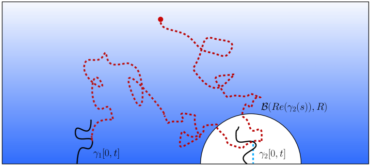
Figure 1: A Brownian motion with $\sigma_{t}<\varrho_{t}$.

The following lemma gives a dynamical interpretation of the weights $\lambda$ and $1-\lambda$.

Lemma 5.3

Let $x(t)=\operatorname{hcap}(\gamma_{1}(0,t])$ and $y(t)=\operatorname{hcap}(\gamma_{2}(0,t])$. Then $x(t)$ and $y(t)$ are differentiable in $t=0$ with

$$\dot{x}(0)=2\lambda\quad\text{and}\quad\dot{y}(0)=2(1-\lambda).$$

Proof.

Let $U_{1},U_{2}$ be the driving functions for the Loewner parametrization ($\gamma_{1},\gamma_{2})$. Without loss of generality we assume that $\Gamma_{1}$ is the left slit, i.e. $U_{1}(t)<U_{2}(t)$ for all $t\in[0,1].$

(i) In a first step we prove $x(t)\geq 2\lambda t$ for all $t\in[0,\tau]$ with some $\tau>0$. Let $n\in{\mathbb{N}}$ and consider the Loewner equation

$$\dot{g}_{t,n}(z)=\frac{2\alpha_{n,\lambda}(t)}{g_{t,n}(z)-U_{1}(t)}+\frac{2(1-\alpha_{n,\lambda}(t))}{g_{t,n}(z)-U_{2}(t)},\quad g_{0,n}(z)=z,$$

where $\alpha_{n,\lambda}$ is defined as in (4.2). Let $K_{n,t}$, $t\in[0,1]$, be the corresponding family of hulls. From Theorem 2.4, we know that ${\mathbb{H}}\setminus K_{n,t}\to{\mathbb{H}}\setminus(\gamma_{1}(0,t]\cup\gamma_{2}(0,t])$ for $n\to\infty$ in the sense of kernel convergence. Let $z_{0}\in(U_{1}(0),U_{2}(0))$ and denote by $z_{n}(t)$ the solution to

$$\dot{z}_{n}(t)=\frac{2\alpha_{n,\lambda}(t)}{z_{n}(t)-U_{1}(t)}+\frac{2(1-\alpha_{n,\lambda}(t))}{z_{n}(t)-U_{2}(t)},\quad z_{n}(0)=z_{0}.$$

It may not exist until $t=1,$ but during its interval of existence we have $z_{n}(t)-U_{2}(t)<0<z_{n}(t)-U_{1}(t)$ and

$$\frac{2}{z_{n}(t)-U_{2}(t)}\leq\dot{z}_{n}(t)\leq\frac{2}{z_{n}(t)-U_{1}(t)}.$$

From this it follows that there exist $\tau,A,B>0$, independent of $n,$ such that $z_{n}(t)$ exists until $t=\tau$ and

$$\max_{s\in[0,\tau]}U_{1}(s)<A<z_{n}(t)<B<\min_{s\in[0,\tau]}U_{2}(s).$$

Thus, for all $n\in{\mathbb{N}}$ and $t\in(0,\tau]$, we can write $K_{t,n}=C_{t,n}\cup D_{t,n}$, where $C_{t,n}$ and $D_{t,n}$ are disjoint subhulls of $K_{t,n}$ with

$${\mathbb{H}}\setminus C_{t,n}\to{\mathbb{H}}\setminus\gamma_{1}(0,t],\quad{\mathbb{H}}\setminus D_{t,n}\to{\mathbb{H}}\setminus\gamma_{2}(0,t].$$

The cluster sets of $C_{t,n}$ and $D_{t,n}$ with respect to $g_{t,n}$ are sets $I_{1}$ and $I_{2}$ respectively with $I_{1}\subset(-\infty,z_{n}(t))$ and $I_{2}\subset(z_{n}(t),+\infty).$ Hence, $C_{t,n}$ is the hull that is growing if and only if $\alpha_{n,\lambda}(t)=1.$

Let $x_{n}(t)=\operatorname{hcap}(C_{n,t})$. Then we get

$$x_{n}\left(\frac{k}{2^{n}}\right)= \sum_{j=1}^{k}\left(x_{n}\left(\frac{j}{2^{n}}\right)-x_{n}\left(\frac{j-1}{2^{n}}\right)\right)=\sum_{j=1}^{k}\left(x_{n}\left(\frac{j-1+\lambda}{2^{n}}\right)-x_{n}\left(\frac{j-1}{2^{n}}\right)\right)$$

$$\underset{\text{Lemma \ref{hcap} (c)}}{\geq} \sum_{j=1}^{k}2\left(\frac{j-1+\lambda}{2^{n}}-\frac{j-1}{2^{n}}\right)=\sum_{j=1}^{k}\frac{2\lambda}{2^{n}}=2\lambda\cdot\frac{k}{2^{n}}$$

for all $n\in{\mathbb{N}}$ and $k\in\{1,...,2^{n}\}$ with $k/2^{n}\leq\tau$.
As $x_{n}(t)\to x(t)$ for every $t\in[0,\tau],$ we conclude that $x(t)\geq 2\lambda t$ for any $t$ of the form $t=k/2^{n}\leq\tau.$ The set of all those $t$ is dense in $[0,\tau]$ and as $x(t)$ is a continuous function, we deduce $x(t)\geq 2\lambda t$ for every $t\in[0,\tau]$.

(ii) In a similar way as in step (i), now utilizing the Loewner equation

$$\dot{h}_{t,n}(z)=\frac{2(1-\alpha_{n,1-\lambda}(t))}{h_{t,n}(z)-U_{1}(t)}+\frac{2\alpha_{n,1-\lambda}(t)}{h_{t,n}(z)-U_{2}(t)}\,,\quad h_{0,n}(z)=z\,,$$

we obtain $y(t)\geq 2(1-\lambda)t$ for all $t\geq 0$ small enough.

(iii) Using the estimates in (i) and (ii), Lemma 5.2 gives

$$2\lambda t\leq x(t)\leq 2\lambda t+{\scriptstyle\mathcal{O}}(t)\qquad\text{for}\quad t\to 0,$$

i.e., $\dot{x}(0)$ exists and $\dot{x}(0)=2\lambda$. In the same way we obtain $\dot{y}(0)=2(1-\lambda)$. ∎

Lemma 5.4

Let $x(t)=\operatorname{hcap}(\gamma_{1}(0,t])$. Then the function $x:[0,1]\to[0,\infty)$ is continuously differentiable with

$$\dot{x}(0)=2\lambda\quad\text{and}\quad\dot{x}(t)>2\lambda\quad\text{for all}\;\;t\in(0,1]\,.$$

In addition,

$$\dot{x}(t)=\frac{2\lambda}{C(x(t),t)}\,,$$

with a continuous function $C:\{(x_{0},t)\,:\,0\leq x_{0}\leq t,0\leq t\leq 1\}\to(0,1]$, which is continuously differentiable w.r.t. $t$.

Proof.

For $j=1,2$ denote by $\theta_{j}(s)$ the parameterization of $\Gamma_{j}$ by its half–plane capacity. Let $t\in[0,1]$ and let $0\leq x_{0}\leq t.$ Then there exists a unique $y_{0}\in[0,1]$ such that $\theta_{1}[0,x_{0}]\cup\theta_{2}[0,y_{0}]$ has half–plane capacity $2t$. Apply the mapping $A:=g_{\theta_{1}[0,x_{0}]}$ on the two slits. We define $\chi(\Delta):=A(\theta_{1}(x_{0}+\Delta))$ for all $\Delta\geq 0$ small enough. Then we have by Lemma 3.1 (b), $\operatorname{hcap}(\chi[0,\Delta])=\operatorname{hcap}(\theta_{1}[0,x_{0}+\Delta])-\operatorname{hcap}(\theta_{1}[0,x_{0}])=2\Delta$. Next we apply the mapping $B:=g_{A(\theta_{2}[0,y_{0}])}.$ Let $\psi(\Delta):=B(\chi(\Delta))$. Now we have

$$\frac{\operatorname{hcap}(\psi[0,\Delta])}{2\Delta}\to B^{\prime}(\chi(0))^{2}\quad\text{for}\quad\Delta\to 0,$$

see [LSW01], Lemma 2.8. Note that $B^{\prime}(\chi(0))^{2}$ depends on $x_{0}$ and $t$ only. So let us define the function $C(x_{0},t):=B^{\prime}(\chi(0))^{2}.$ $C$ has the following properties:

• $(x_{0},t)\mapsto C(x_{0},t)$ is continuous: $A$ and $\chi(0)$ depend continuously on $x_{0}$. Furthermore, $y_{0}$ depends continuously on the pair $(x_{0},t),$ so $B$ depends continuously on $(x_{0},t)$ as well as $C(x_{0},t)=B^{\prime}(\chi(0))^{2}.$

• $C$ is continuously differentiable with respect to $t$: For fixed $x_{0}$, both the value $y_{0}$ and the mapping $B$ are continuously differentiable with respect to $t,$ see section 4.6.1 in [Law05]. Hence, as $\chi(0)$ is fixed, also $B^{\prime}(\chi(0))$ is continuously differentiable w.r.t. $t$.

• $C(x_{0},t)\in(0,1)$ for all $0\leq x_{0}<t\leq 1$: see Proposition 5.15 in [Law05].

Now we look at the case $x_{0}=x(t).$ Then $x(t+h)-x(t)=\operatorname{hcap}(\chi[0,\Delta(h)])=2\Delta(h)$ and we know that

$$\lim_{h\downarrow 0}\frac{\operatorname{hcap}(\psi[0,\Delta(h)])}{h}=2\lambda.$$

This follows by applying Lemma 5.3 to the slit $g_{t}(\Gamma_{1}\setminus\gamma_{1}[0,t])$. Thus

$$\lim_{h\downarrow 0}\frac{x(t+h)-x(t)}{h}=\lim_{h\downarrow 0}\frac{2\Delta(h)}{h}=\lim_{h\downarrow 0}\frac{2\Delta(h)\cdot\operatorname{hcap}(\psi[0,\Delta(h)])}{\operatorname{hcap}(\psi[0,\Delta(h)])\cdot h}=\frac{2\lambda}{C(x(t),t)}.$$

Hence, the right derivative of $x(t)$ exists and is continuous, so $x(t)$ is continuously differentiable, see Lemma 4.3 in [Law05], and

$$\dot{x}(t)=\frac{2\lambda}{C(x(t),t)}\,.$$

∎

6 Proof of Theorem 1.1, Part II (Uniqueness)

Let $\nu,\mu\in[0,1]$ be constant weights and $U_{1},U_{2},V_{1},V_{2}:[0,1]\to{\mathbb{R}}$ be continuous driving functions such that the solutions $g_{t}$ and $h_{t}$ of

$$\dot{g}_{t}=\frac{2\nu}{g_{t}-U_{1}(t)}+\frac{2(1-\nu)}{g_{t}-U_{2}(t)},\,g_{0}(z)=z\quad\text{and}\quad\dot{h}_{t}=\frac{2\mu}{h_{t}-V_{1}(t)}+\frac{2(1-\mu)}{h_{t}-V_{2}(t)},\,h_{0}(z)=z$$

satisfy $g_{1}=h_{1}=g_{\Gamma_{1}\cup\Gamma_{2}}.$

Assume $\nu>\mu$. Let $x_{1}(t)$ and $x_{2}(t)$ be the half–plane capacities of the generated part of $\Gamma_{1}$ at time $t$ with respect to $g_{t}$ and $h_{t}$, and let $y_{1}(t)$ and $y_{2}(t)$ be the corresponding half–plane capacities of $\Gamma_{2}.$ Then $\dot{x}_{1}(0)=\nu>\mu=\dot{x_{2}}(0)$ by Lemma 5.3. Consequently, $x_{1}(t)>x_{2}(t)$ for all $t\geq 0$ small enough. Since $x_{1}(1)=\operatorname{hcap}(\Gamma_{1})=x_{2}(1)$, there is a first time $\tau\in(0,1]$ such that $x_{1}(\tau)=x_{2}(\tau)$. Then $x_{1}(t)>x_{2}(t)$ for every $t\in(0,\tau)$, so $\dot{x}_{1}(\tau)\leq\dot{x}_{2}(\tau)$. On the other hand, Lemma 5.4 shows that

$$\dot{x}_{1}(\tau)=\frac{2\nu}{C(x_{1}(\tau),\tau)}>\frac{2\mu}{C(x_{2}(\tau),\tau)}=\dot{x}_{2}(\tau)\,,$$

a contradiction. Hence we know that $\nu\leq\mu$. By switching the roles of $\nu$ and $\mu$, we deduce $\nu=\mu$.

Next, again with the help of Lemma 5.4, we see that both functions $x_{1}$ and $x_{2}$ are solutions to the same initial value problem,

$$\dot{x}(t)=\frac{2\mu}{C(x(t),t)}\,,\quad x(0)=0\,,$$

where $(x_{0},t)\mapsto 2\mu/C(x_{0},t)$ is continuous, positive and Lipschitz continuous in $t$. However, the solution to such a problem is unique according to Theorem 2.7 in [CP03]. Hence $x_{1}=x_{2}$ and also $y_{1}=y_{2}$, so we have

$$H(t):=\theta_{1}[0,x_{1}(t)]\cup\theta_{2}[0,y_{1}(t)]=\theta_{1}[0,x_{2}(t)]\cup\gamma_{2}[0,y_{2}(t)]$$

for all $t.$ Using the geometric meaning of the driving functions (see Section 2), we finally get $U_{j}(t)=g_{H(t)}(\theta_{j}(x_{1}(t))=g_{H(t)}(\theta_{j}(x_{2}(t))=V_{j}(t)$ for $j=1,2$. This completes the proof of the uniqueness statement of Theorem 1.1.

University of Würzburg, Department of Mathematics, 97074 Würzburg, Germany
E-mail addresses:
roth@mathematik.uni-wuerzburg.de,
sebastian.schleissinger@mathematik.uni-wuerzburg.de

References

- [BBK05] M. Bauer, D. Bernard, and K. Kytölä, Multiple Schramm-Loewner evolutions and statistical mechanics martingales, J. Stat. Phys. 120 (2005), no. 5-6, 1125–1163.
- [BCD12] F. Bracci, M. D. Contreras, S. Díaz-Madrigal, Evolution families and the Loewner equation. I: The unit disc, J. Reine Angew. Math. 672 (2012), 1–37.
- [BS] Ch. Böhm and S. Schleißinger, preprint.
- [Car03] J. Cardy, Stochastic Loewner evolution and Dyson’s circular ensembles, J. Phys. A 36 (2003), no. 24, L379–L386.
- [CM02] L. Carleson and N. Makarov, Laplacian path models, J. Anal. Math. 87 (2002), 103–150, Dedicated to the memory of Thomas H. Wolff.
- [CP03] J. Angel Cid and Rodrigo López Pouso, On first-order ordinary differential equations with nonnegative right-hand sides, Nonlinear Anal. 52 (2003), no. 8, 1961–1977.
- [Dub07] J. Dubédat, Commutation relations for Schramm-Loewner evolutions, Comm. Pure Appl. Math. 60 (2007), no. 12, 1792–1847.
- [DV11] M. A. Durán and G.–L. Vasconcelos, Fingering in a channel and tripolar Loewner evolutions, Phys. Rev. E 84 (2011), 051602.
- [FR75] W. H. Fleming and R. W. Rishel, Deterministic and Stochastic Optimal Control, Springer, 1975.
- [GB92] V. V. Goryainov and I. Ba, Semigroup of conformal mappings of the upper half–plane into itself with hydrodynamic normalization at infinity, Ukrainian Math. J. 44 (1992), no. 10, 1209–1217.
- [Gra07] K. Graham, On multiple Schramm–Loewner evolutions, Journal of Statistical Mechanics: Theory and Experiment 2007 (2007), no. 03.
- [GS08] T. Gubiec and P. Szymczak, Fingered growth in channel geometry: a Loewner-equation approach, Phys. Rev. E (3) 77 (2008), no. 4, 041602, 12.
- [GM13] P. Gumenyuk and A. del Monaco, Chordal Loewner equation, eprint arxiv:1302.0898v2
- [Jur97] V. Jurdjevic, Geometric Control Theory, Cambrdige Univ. Press, 1997.
- [KL07] M. J. Kozdron and G. F. Lawler, The configurational measure on mutually avoiding SLE paths, Universality and renormalization, Fields Inst. Commun., vol. 50, Amer. Math. Soc., Providence, RI, 2007, pp. 199–224.
- [KSS68] P. P. Kufarev, V. V. Sobolev, and L. V. Sporyševa, A certain method of investigation of extremal problems for functions that are univalent in the half–plane, Trudy Tomsk. Gos. Univ. Ser. Meh.-Mat. 200 (1968), 142–164.
- [LLN09] S. Lalley, G. F. Lawler, and H. Narayanan, Geometric interpretation of half–plane capacity, Electron. Commun. Probab. 14 (2009), 566–571.
- [Law05] G. F. Lawler, Conformally invariant processes in the plane, Mathematical Surveys and Monographs, vol. 114, American Mathematical Society, Providence, RI, 2005.
- [LSW01] G. F. Lawler, O. Schramm, and W. Werner, Values of Brownian intersection exponents. I: Half–plane exponents, Acta Math. 187, No. 2 (2001), 237–273.
- [LMR] J. Lind, D.E. Marshall, and S. Rohde, Collisions and spirals of Loewner traces, Duke Math. J. 154 (2010), no. 3, 527–573.
- [LR] J. Lind and S. Rohde, Spacefilling curves and phases of of the Loewner equations, Indiana Univ. Math. J., to appear, eprint arXiv:1103.0071.
- [Loe23] K. Löwner, Untersuchungen über schlichte konforme Abbildungen des Einheitskreises. I., Math. Ann. 89 (1923), 103–121.
- [Pes36] E. Peschl, Zur Theorie der schlichten Funktionen, J. Reine Angew. Math. 176 (1936), 61–94.
- [Pro93] D. V. Prokhorov, Reachable set methods in extremal problems for univalent functions, Saratov University, 1993.
- [RW] S. Rohde and C. Wong, Half–plane capacity and conformal radius, Proc. Amer. Math. Soc., to appear, eprint arXiv:1201.5878.
- [RR94] M. Rosenblum and J. Rovnyak, Topics in Hardy Classes and Univalent Functions, Birkhäuser 1994.
- [Sch00] O. Schramm, Scaling limits of loop-erased random walks and uniform spanning trees, Isr. J. Math. 118 (2000), 221–288.