On the origin of X-ray spectra in luminous blazars

Abstract

Gamma-ray luminosities of some quasar-associated blazars imply jet powers reaching values comparable to the accretion power even if assuming very strong Doppler boosting and very high efficiency of gamma-ray production. With much lower radiative efficiencies of protons than of electrons, and the recent reports of very strong coupling of electrons with shock-heated protons indicated by Particle-in-Cell (PIC) simulations, the leptonic models seem to be strongly favored over the hadronic ones. However, the electron-proton coupling combined with the ERC (External-Radiation-Compton) models of gamma-ray production in leptonic models predict extremely hard X-ray spectra, with energy indices $\alpha_{x}\sim 0$.This is inconsistent with the observed 2-10 keV slopes of blazars, which cluster around $\alpha_{x}\sim 0.6$. This problem can be resolved by assuming that electrons can be efficiently cooled down radiatively to non-relativistic energies, or that blazar spectra are entirely dominated by the SSC (Synchrotron-Self Compton) component up to at least 10 keV. Here, we show that the required cooling can be sufficiently efficient only at distances $r<0.03$ pc. SSC spectra, on the other hand, can be produced roughly co-spatially with the observed synchrotron and ERC components, which are most likely located roughly at a parsec scale. We show that the dominant SSC component can also be produced much further than the dominant synchrotron and ERC components, at distances of $\gtrsim 10$ parsecs. Hence, depending on the spatial distribution of the energy dissipation along the jet, one may expect to see $\gamma$-ray/optical events with either correlated or uncorrelated X-rays. In all cases the number of e⁺e^- pairs per proton is predicted to be very low. The direct verification of the proposed SSC scenario, and particularly the question of the co-spatiality of the SSC component with other spectral components, requires sensitive observations in the hard X-ray band. This is now possible with the deployment of the NuSTAR satellite, providing the required sentitivity to monitor the details of the hard X-ray spectra of blazars in the range where the ERC component is predicted to start dominating over the SSC component.

1 Introduction

Images of extended jets in radio-galaxies and quasars show that jet energy is dissipated more or less smoothly over all spatial scales. But in powerful, FR II type radio sources, a large fraction of energy is very efficiently transmitted up to hundreds of kiloparsecs and dissipated there in terminal shocks. Studies of energy content of radio lobes indicate that they are powered by jets at rates sometimes comparable or even exceeding the accretion power (Rawlings & Saunders 1991; Punsly 2007; Fernandes et al. 2011). Such extreme energetics is independently confirmed by studies of luminous blazars (Ghisellini et al. 2010; Ghisellini et al. 2011). These objects, with relativistically boosted jets pointing almost exactly at us, allow tracing the jet structure at parsec/subparsec distances from the black hole. Their structure on such scales is explored by multiwavelength studies of variability. However, the multi-band time series of blazars are complex, precluding a consensus regarding the physics of AGN jets — their power, matter content, magnetization, cross-sectional structure, etc. This is not surprising, given that on such scales a variety of processes may contribute to the jet evolution and its nonthermal activity. Presumably, a conversion from the magnetic to the matter energy flux dominated flow takes place already at subparsec scales (Sikora et al. 2005). This conversion could be triggered by MHD instabilities, and governed by efficiency of the magnetic reconnection (Begelman 1998; Giannios & Spruit 2006; Lyubarsky 2010). Non-steady and non-axisymmetric jet launching, as is predicted by the scenario which involves MCAF (Magnetically-Choked Accretion Flows; McKinney et al. 2012), may strongly amplify these processes and generate strong internal shocks (Spada et al. 2001). Finally, due to interaction of the flow with external medium, oblique/reconfinement shocks are expected to be formed (Daly & Marscher 1988; Komissarov & Falle 1997; Nalewajko & Sikora 2009).

Given the complexity of the jet structure, one might expect that dissipation processes in blazars are not limited to a single zone, but rather they operate independently over two or more sites at once, and with different and possibly variable efficiencies. Hence, since different radiation spectra are produced at different sites, one might expect a broad range of correlations and time lags between different spectral bands (see, e.g., Janiak et al. 2012). However, attempts to use multiwavelength observations to associate the specific spectral portions with a given dissipation site are still hampered by insufficient models of particle acceleration, particularly regarding the behavior electrons in the presence of ions. Electrons need to tap a significant fraction of dissipated energy in order to explain large luminosities of blazars, otherwise this energy would go to protons which only under very specific conditions can radiate efficiently, or can efficiently trigger processes leading to the production of secondary electrons/positrons (Sikora 2011). A variety of mechanisms were suggested to preheat electrons up to the thermal level of the shocked protons, and allow them to participate in the diffusive shock acceleration process (e.g. Hoshino et al. 1992; Hoshino & Shimada 2002). Recent Particle-In-Cell (PIC) simulations demonstrated strong electron-proton coupling in shocks (Sironi & Spitkovsky 2011), and thus confirmed the expected potential of the leptonic models to generate very luminous events in blazars.

In order to map the structure of nuclear jets in quasars, it is also necessary to know the geometry of external radiation sources, which provide seed photons for the ERC production of $\gamma$-rays. At least the structures responsible for broad emission lines are expected to be stratified and flattened (see Wills & Brown 1986; Krolik et al. 1991; Horne et al. 1991; Arav et al. 1998; Gaskell et al. 2007; Czerny & Hryniewicz 2011). Both strong proton-electron coupling and such geometries are critical ingredients in our approach to establish the sites of the observed radiation spectra in luminous blazars.

This paper is organized as follows: in Section 2, we discuss the implications of very large $\gamma$-ray luminosities and of strong electron-proton coupling for radiative scenarios; Section 3 formulates the connection of the energy dissipation efficiency with the average electron injection energy and e⁺e^--pair content; in Section 4, we investigate possible mechanismsof X-ray production in luminous blazars in light of the strong electron-proton coupling and the large electron injection energy. Our main results are discussed in Section 5 and summarized in Section 6.

2 Jet powers in luminous $\gamma$-ray blazars

The radiative output of luminous blazars associated with FSRQs (Flat-Spectrum Radio Quasars) is often strongly dominated by $\gamma$-rays. For observers located at an angle $1/\Gamma$ to the jet axis, the apparent $\gamma$-ray luminosity of such objects is

$$L_{\gamma}\simeq\eta_{\gamma}\eta_{p/e}\eta_{\rm diss}\,\Gamma^{2}L_{j,0}\,,$$ (1)

where $\eta_{\rm diss}$ is the overall dissipation efficiency, $\eta_{p/e}$ is the fraction of dissipated energy channeled to accelerated protons or electrons, $\eta_{\gamma}$ is the fraction of energy of the accelerated particles emitted in the $\gamma$-ray band and $L_{j,0}$ is the jet power before dissipation region. Depending on whether $\gamma$-rays are produced by directly accelerated/heated electrons (leptonic models) or by protons and products of their interactions with photons and/or matter (hadronic models), $\eta_{p/e}=\eta_{e}$ or $\eta_{p}$, respectively.

Noting that the maximal jet power is limited by the accretion power (McKinney et al. 2012 and refs. therein):

$$\frac{L_{j,0}}{\dot{M}_{d}c^{2}}=\frac{L_{\gamma}\epsilon_{d}}{\eta_{\gamma}\eta_{p/e}\eta_{\rm diss}\Gamma^{2}L_{d}}\,\lesssim 1\,,$$ (2)

which gives

$$\eta_{\gamma}\eta_{p/e}\eta_{\rm diss}\gtrsim\frac{1}{4}\frac{L_{\gamma,49}(\epsilon_{d}/0.3)}{(\Gamma/20)^{2}(L_{d}/0.3L_{\rm Edd})M_{\rm BH,9}}\,,$$ (3)

where $\dot{M}_{d}$ is the disk accretion rate, $L_{d}$ is the accretion disk luminosity, $\epsilon_{d}$ is the disk radiative efficiency, and $M_{\rm BH,9}=M_{\rm BH}/10^{9}M_{\odot}$. This means that all efficiencies must be high. However there are certain constraints on some of them. Very demanding energetics of extended, FR II radio sources (Rawlings & Saunders 1991; Punsly 2007; Fernandes et al. 2011) indicates that the jet cannot lose most of its energy before reaching the terminal shocks in hot spots, therefore, $\eta_{\rm diss}$ is expected to be less than $\sim 0.5$. Even stronger constraints on $\eta_{\rm diss}$ are provided by models of reconfinement/oblique shocks (Nalewajko 2012) as well as internal, relativistically propagating shocks (Spada et al. 2001). Regarding $\eta_{p}$ no severe constraints exist, at least in the shock models. Likewise, given a very strong coupling between protons and electrons in shocked plasmas, as indicated by PIC simulations (Sironi & Spitkovsky 2011), no severe constraints are imposed on $\eta_{e}$. For $n_{e}=n_{p}$, they can share their total energy equally, e.g. $\eta_{e}\simeq\eta_{p}\simeq 0.5$. Efficiency of the gamma-ray production, $\eta_{\gamma}$, may have a very broad range depending on a distance from the black hole and on the particle injection spectrum. Efficient cooling of protons is possible only if they are injected very close to the black hole, at $r<100R_{g}$, and if most of them are injected with ultrarelativistic energies (Sikora 2011). In the case of the power-law injection the latter condition implies the injection spectral index $p<1$.

In leptonic models, $\gamma$-rays can be efficiently produced by relativistic electrons up to several parsecs. Because of the strong electron-proton coupling, electrons are preheated up to relativistic energies with the quasi-Maxwellian distribution with similar average energy as protons. The Maxwellian distribution naturally explains the formation of very hard low-energy tail of injected electrons. All the above favors the leptonic radiative models, and only such will be investigated below.

3 Energy dissipation efficiency and average electron injection energy

Blazars can be powered by kinetic energy of cold protons, as well as by various forms of internal energy – magnetic or macro-turbulent. The kinetic one can be dissipated via the reconfinement/oblique shocks (Daly & Marscher 1988; Komissarov & Falle 1997; Nalewajko & Sikora 2009), the macro-turbulent one – via the internal shocks (Spada et al. 2001), and the magnetic one – via the reconnection (Lovelace, Newman & Romanova 1997; Lyubarsky 2010; Nalewajko et al. 2011). While the dissipation of jet energy in a reconfinement shock does not involve motion of the dissipation sites, internal shocks and reconnection layers form a sequence of moving sites. However, noting that the blazar high states, albeit very variable, last usually much longer than the time scale of passing of the flow through the distance range where most of the blazar radiation is produced, one may approximate the dissipation zone as steady-state in all cases.

Assuming $n_{e}/n_{p}\ll m_{p}/m_{e}$ one can write the jet power in the form $L_{j}=L_{p}+L_{\rm int}$, where $L_{p}$ is the flux of kinetic energies of cold protons,

$$L_{p}=(dN_{p}/dt)m_{p}c^{2}(\Gamma-1)\,,$$ (4)

and $L_{\rm int}$ is the flux of internal energies. For the conserved proton number flux, $dN_{p}/dt={\rm const}$, that provides formula for an efficiency of the jet energy dissipation within a given region

$$\eta_{\rm diss}=\frac{(L_{j,0}-L_{j})}{L_{j,0}}=1-\frac{(\Gamma-1)(1+\sigma)}{(\Gamma_{0}-1)(1+\sigma_{0})}\,,$$ (5)

where $\sigma=L_{\rm int}/L_{p}$, $\Gamma$ is the jet Lorentz factor, and quantities with the subscript ’0’ are the initial values of the variable / parameter.

3.1 Average energy of injected electrons

Electrons tap energy at a rate

$$\frac{dN_{e,\rm inj}}{dt}\bar{\gamma}_{\rm inj}\,m_{e}c^{2}\Gamma=\eta_{e}\eta_{\rm diss}L_{j,0}\,,$$ (6)

where $\bar{\gamma}_{\rm inj}m_{e}c^{2}\Gamma$ is the average energy gained by an electron and $dN_{e,\rm inj}/dt=\int_{\gamma_{\rm min}}^{\gamma_{\rm max}}{Q_{\gamma}\,{\rm d}\gamma}$ is the electron injection rate. Assuming that each electron is accelerated once gives

$$\frac{dN_{e,inj}}{dt}=\frac{dN_{e}}{dt}=\frac{n_{e}}{n_{p}}\,\frac{dN_{p}}{dt}\,,$$ (7)

and combining Eqs.(6), (7) and (4) we obtain that for $\Gamma\gg 1$:

$$\bar{\gamma}_{\rm inj}=\frac{n_{p}m_{p}}{n_{e}m_{e}}\,\frac{\eta_{e}\eta_{\rm diss}}{(1-\eta_{\rm diss})}\,(1+\sigma)\,.$$ (8)

3.2 Pair content

By modeling the blazar spectra, one can estimate the value of $\bar{\gamma}_{\rm inj}$, and using Eq. (8) one may estimate the e⁺e^--pair content:

$$\frac{n_{e}}{n_{p}}=\left(\frac{m_{p}}{m_{e}}\right)\left(\frac{\eta_{\rm diss}}{1-\eta_{\rm diss}}\right)\,\frac{(\eta_{e}/0.5)(1+\sigma)}{\bar{\gamma}_{\rm inj}}\,,$$ (9)

For $\sigma<1$, $\eta_{\rm diss}<0.5$, and $\eta_{e}=0.5$ (implied by the strong electron-proton coupling), Eq. (9)
gives $n_{e}/n_{p}<10$ for $\bar{\gamma}_{\rm inj}=100$, and $n_{e}\sim n_{p}$ for $\bar{\gamma}_{\rm inj}=500$. Similar constraint on a pair content has been derived, but using different arguments, by Ghisellini & Tavecchio (2012). 

4 Spectral consequences of the strong proton-electron coupling

Strong coupling between protons and electrons implies the break in the electron injection spectrum just below $\bar{\gamma}_{\rm inj}$ and formation of an extremely hard low-energy tail, with the index $p<1$ ($Q_{\gamma}\propto\gamma^{-p}$). In the slow-cooling regime, i.e. where the electron energy losses are dominated by adiabatic losses, such an injection function leads to the low portion of the electron-energy-distribution with the slope $s=1$ ($N_{\gamma}\propto\gamma^{-s}$), and radiation flux index $\alpha=0$ ($F_{\nu}\propto\nu^{-\alpha}$). Since typically the soft/mid X-ray spectra in luminous blazars have much softer slopes ($\alpha_{x}\sim 0.6$: Abdo et al. 2010a; Ghisellini et al. 2011; Giommi et al. 2012), they cannot be low energy tails of the ERC spectral component if produced in the slow cooling regime. One can exclude also production of such spectra by superposition of the SSC component with the very hard low-energy ERC component, because that would require fine tuning of model parameters, particularly if the SSC spectrum in the X-ray band has a slope $\alpha>1$. But there are still two other options: (i) production of soft/mid X-rays by the ERC process in the fast cooling regime; (ii) the SSC process with the luminosity peak at $h\nu_{x}\gtrsim 30$ keV. Both are examined below.

4.1 X-ray spectra as the low energy tail of the ERC component in the fast cooling regime?

Due to efficient radiative losses, the low-energy portions of the ERC spectra extend down to $h\nu_{c}\simeq\gamma_{c}^{2}\Gamma^{2}\nu_{\rm ext}$ with the slope $\alpha\simeq 0.5$, where

$$\gamma_{c}\simeq\frac{m_{e}c^{2}}{\sigma_{T}}\,\frac{\Gamma}{ru_{\rm ext}^{\prime}}$$ (10)

is the cooling break, and

$$u_{\rm ext}^{\prime}={g_{u}\xi L_{d}\Gamma^{2}\over 4\pi r^{2}c}\,,$$ (11)

is the energy density of the external radiation in the jet co-moving frame, $\xi$ is the fraction of the accretion disc luminosity, $L_{d}$, reprocessed in the BLR and dusty torus, and $g_{u}$ is the numerical factor which depends on the geometry of the external radiation sources. For stratified and flattened source geometries the value of $g_{u}$ is expected to be of the order of $0.1$ (see Appendix A and Fig. A1). Since for $\gamma<\gamma_{c}$ the adiabatic losses start to dominate and the spectrum breaks down to $\alpha\sim 0$, in order to explain the much softer observed X-ray spectra, radiative cooling of electrons should be efficient down to their lowest energies. Having from Eqs. (10) and (11)

$$\gamma_{c}\simeq\frac{r}{4.3\times 10^{16}\,{\rm cm}}\,\frac{1}{(g_{u}/0.1)(\xi/0.1)(\Gamma/20)L_{d,47}}\,,$$ (12)

one can see that electrons can be cooled down to $\gamma_{c}\sim 1$ when the event is located at $r\lesssim 0.01$ pc.

In such a case, one could expect a bulk-Compton (BC) excess in the X-ray spectra (Begelman & Sikora 1987). At such close proximity to the accretion disk, the ERC cooling is dominated by Comptonization of the direct accretion disk radiation (Dermer & Schlickeiser 2002). Noting that typical energy of external photons at these distances is of the order $\sim 1$ eV, one can find the observed energy of the BC feature:

$${\rm h}\nu_{\rm BC}\sim\frac{0.4(\Gamma/20)^{2}}{(1+z)}\,{\rm keV}\,.$$ (13)

Such a feature cannot be detected at cosmological distances, unless $\Gamma>20$.

One might also consider electron cooling at somewhat larger distances, taking into account the uncertainties of parameters $g_{u}$ and $\xi$. Because high ionization lines, which are produced closer to the black hole than the low ionization lines, form much less flattened geometry, the value of $g_{u}$ in the inner BLR can be larger than adopted by us fiducial value $0.1$. Also the value of $\xi$ can be larger than 0.1 according to some analyses (Kollatschny & Zetzl 2013). Noting these uncertainties, one cannot exclude the possibility that both parameters are underestimated by a factor few, and that the distance at which $\gamma_{c}$ reaches value $\sim 1$ is $\sim 0.1$ pc, where external radiation is dominated by the broad emission lines. However in such a case, energy of the BC feature is predicted to be located at

$${\rm h}\nu_{\rm BC}\sim\frac{4(\Gamma/20)^{2}}{(1+z)}\,~{}[{\rm keV}]\,.$$ (14)

Noting that typical Lorentz factors implied by ERC(BLR) models are $\Gamma\sim 15$ (see, e.g., Celotti & Ghisellini 2008, Table A1) and that X-ray spectra of most FSRQs show no steepening nor flattening in the 0.1-2.4 keV band (Sambruna 1997; Lawson & McHardy 1998), that prediction seems to contradict with observations.

4.2 Production of X-ray spectra with $\alpha<1$ by the SSC process

When the electron injection function at $\gamma>\bar{\gamma}_{\rm inj}$ has a slope $2<p<3$, the production of radiation around the spectral component maxima (hereafter: spectral peaks) will be dominated by electrons with energies around either $\bar{\gamma}_{\rm inj}$ or $\gamma_{c}$. Hence, noting that the distance at which both values are equal is

$$r_{\rm ci} \equiv r(\gamma_{c}=\bar{\gamma}_{\rm inj})=$$

$$= 2.2\times 10^{19}\,\left(\frac{\Gamma}{20}\right)\left(\frac{g_{u}}{0.1}\right)\left(\frac{\xi}{0.1}\right)\left(\frac{\bar{\gamma}_{\rm inj}}{500}\right)L_{d,47}\,[{\rm cm}]\,,$$

and that cooling break energy increases with the distance from the black hole, the spectral peaks will be determined by electrons with $\gamma\sim\bar{\gamma}_{\rm inj}$ at distances $r<r_{\rm ci}$, and by electrons with $\gamma\sim\gamma_{c}$ at distances $r>r_{\rm ci}$. In case of $p>3$ the spectral peaks will be associated with the injection energy over all distances.

4.2.1 Association of the SSC peak with the average electron energy injection

Electrons injected with the sharp, low energy break at $\bar{\gamma}_{\rm inj}$ and the slope $p>2$ at larger energies produce SSC spectral component with the peak at

$$\nu_{\rm ssc,i}\simeq\bar{\gamma}_{\rm inj}^{2}\nu_{\rm syn,i}=c_{B}B^{\prime}\bar{\gamma}_{\rm inj}^{4}\Gamma\,,$$ (16)

where $c_{B}\simeq 3.7\times 10^{6}\,{\rm Gauss}^{-1}s^{-1}$.

Assuming that magnetic field intensity decreases with the distance like $B^{\prime}\propto 1/r$, and is scaled according to the relation $u_{B}^{\prime}=u_{\rm ext}^{\prime}/q$, where $q\equiv L_{\gamma}/L_{\rm ir/opt}$, we obtain

$$B^{\prime}=\frac{\Gamma}{r}\,\sqrt{\frac{2g_{u}\xi L_{d}}{\pi cq}}\,.$$ (17)

The requirement that X-ray spectra are produced by the SSC process with $\alpha_{x}<1$ up to tens of keV’s (Ajello et al. 2009) implies the location of the SSC peak in the range $10-100$ keV. Then, Eqs. (16) and (17) give

$$\bar{\gamma}_{\rm inj} \simeq 660\,r_{\rm pc}^{1/4}\,\left(\frac{{\rm h}\nu_{\rm ssc,i}}{30{\rm keV}}\right)\,\left[\frac{(q/10)}{(g_{u}/0.1)(\xi/0.1)L_{d,47}}\right]^{1/4}\times$$ (18)

$$\times\left(\frac{\Gamma}{20}\right)^{-1/2}\,.$$

where $r_{\rm pc}\equiv r/1$ pc. For such injection energies, for $n_{e}=n_{p}$ and $\sigma<1$, Eq.(8) implies the energy dissipation efficiency $\eta_{\rm diss}\sim 42\%$ at $r\sim 1$ pc.

4.2.2 Association of the SSC peak with the cooling break

For $r>r_{\rm ci}$, the SSC peak is located at

$$\nu_{\rm ssc,peak}=\nu_{\rm ssc,c}=c_{B}B\Gamma\gamma_{c}^{4}\,.$$ (19)

This equation, together with Eqs. (4.2), (12) and (17), gives the distance at which the SSC peak associated with the cooling break will be located at ${\rm h}\nu_{\rm ssc,c}=30$ keV:

$$r_{\rm ssc,c} \simeq 1.3\times 10^{20}\,\left(\frac{\Gamma}{20}\right)^{2/3}\left[\left(\frac{g_{u}}{0.1}\right)\left(\frac{\xi}{0.1}\right)L_{d,47}\right]^{7/6}\times$$ (20)

$$\times\left(\frac{q}{10}\right)^{1/6}\,\left(\frac{{\rm h}\nu_{\rm ssc,c}}{30{\rm keV}}\right)^{1/3}\,[{\rm cm}]\,;$$

and the value of the cooling break energy:

$$\gamma_{c} \simeq 3.0\times 10^{3}\,\left(\frac{\Gamma}{20}\right)^{-1/3}\left[\left(\frac{g_{u}}{0.1}\right)\left(\frac{\xi}{0.1}\right)L_{d,47}\right]^{1/6}\times$$ (21)

$$\times\left(\frac{q}{10}\right)^{1/6}\left(\frac{{\rm h}\nu_{\rm ssc,c}}{30{\rm keV}}\right)^{1/3}\,.$$

4.3 Can the observed X-ray spectra be produced co-spatially with $\gamma$-rays and optical radiation?

Correlations of optical and $\gamma$-ray variabilities, often observed in FSRQs, suggest a co-spatiality of their emission zones. In the framework of the ERC model for $\gamma$ rays, this allows to use two observables — $q=L_{\gamma}/L_{\rm IR/opt}$ and $w=\nu_{\rm\gamma,peak}/\nu_{\rm IR/opt}$ — to estimate the location of that zone. This comes from relations

$$q=\frac{L_{\gamma}}{L_{\rm IR/opt}}\simeq\frac{u_{\rm ext}^{\prime}}{u_{B}^{\prime}}\,$$ (22)

and

$$w=\frac{\nu_{\rm\gamma,peak}}{\nu_{\rm IR/opt}}=\frac{\nu_{\rm erc}}{\nu_{\rm syn}}\,.$$ (23)

These equations imply two possible regions where a co-spatial ERC and synchrotron emission may take place: one within the BLR, where ERC is seeded by broad emission lines; and one at distances larger by factor $\nu_{\rm BLR}/\nu_{\rm HD}\sim 30$, where ERC seeding is provided by IR photons from the dusty torus (Sikora et al. 2009 and refs. therein). Such a ‘degeneracy’, in the sense of the same synchrotron and ERC spectral peak locations at two different distances, is broken for the SSC component. This is because the production of spectral peaks at these two distances involves different – by a factor of $\sqrt{30}$ – energies of electrons. And noting that $\nu_{\rm ssc}\propto{\gamma}^{4}B^{\prime}$ where $B^{\prime}\propto 1/r$, we expect very different locations of the SSC peaks. While in the outer dust region domain the SSC peak can be produced at $\sim 30$ keV energies, within the BLR the SSC peaks are located at $\sim\left(\sqrt{30}\right)^{4}/30=30$ times lower energies, i.e. at $\sim 1$ keV.

Hence, within the BLR the X-ray spectra with $\alpha_{x}<1$ cannot be produced by the SSC process operating co-spatially with the gamma-ray emission via ERC. In order to reproduce the entire broad-band spectra with IR/optical and $\gamma$-rays produced in BLR, the X-rays must originate either from the SSC process located at distances $r>r_{\rm ci}>r_{\rm BLR}$ (see 4.2.2), or from the low energy tail of the ERC component located at distances $r<r_{\rm BLR}$ (see 4.1). Since the time scales of the X-ray variations are usually longer than those of the $\gamma$-ray variations, larger distances of the X-ray production are more likely. Furthermore, $\gamma$-rays produced co-spatially with X-rays at $r>r_{\rm ic}$ can explain the VHE radiation observed in some luminous blazars (3C 279: Aleksić et al. 2011a; PKS 1222+216: Aleksić et al. 2011b; Tanaka et al. 2011; PKS 1510-089: H.E.S.S. Collaboration 2013; Barnacka et al. 2013), which in the BLR is expected to be strongly absorbed (see Tavecchio & Ghisellini 2012 and refs. therein). At the same time, a contribution from the synchrotron emission produced at $r>r_{\rm ic}$ to sub-mm radiation can explain variations in this band on the times scales of weeks (Sikora et al. 2008), and can suppress the variability amplitude in the FIR band (Nalewajko et al. 2012). Such a two-zone model can be verified by searching for correlations between sub-mm, X-ray, and TeV variabilities.

5 Discussion

The origin of X-ray emission in FSRQs was long ago recognized as an important probe of the jet physics with implications for the nature of the gamma-ray emission. In the EC scenario, the X-ray emission would probe the low-energy (transrelativistic) electrons, and there was a hope that X-ray spectra would reveal a so-called bulk-Compton component produced by a population of cold electrons (Begelman & Sikora 1987). Lack of strong observational evidence of the bulk-Compton feature (although see Kataoka et al. 2008, Ackermann et al. 2012) places constraints on the e⁺e^- pair content, according to which $n_{e}/n_{p}<30$ (Sikora & Madejski 2000).

As we demonstrate in Section 3.2, the pair content is further constrained, down to $n_{e}/n_{p}<$ a few, if noting that the electrons and protons are strongly coupled, according to PIC simulations of relativistic shocks (Sironi & Spitkovsky 2011). The main part of this paper is devoted to the spectral consequences of such a coupling. The $e-p$ coupling implies extremely hard low-energy tails of the electron injection function, and therefore extremely efficient radiative cooling is required to explain the X-ray spectra with slopes clustered around $\alpha_{x}\sim 0.6$. As shown in Section 4.1, such spectra can be reproduced only at very small distances from the black hole, where seeding of the ERC process is dominated by direct radiation from the accretion disk.

Another option is that the production of X-rays is dominated by the SSC process (Kubo et al. 1995). As we demonstrate in Section 4.2.1, consistency of the theoretical SSC spectral slopes with the observed X-ray indices is achievable provided that electrons contributing to the spectral peaks have energies $\gamma_{\rm peak}>500$. Such energies are too large to explain the location and separation of the synchrotron and ERC peaks in the BLR, but are of the same order as those predicted by the models which locate the blazar zone on distance scales of the dusty torus. Hence, on these larger scales the X-ray spectra can be produced co-spatially with the optical emission and $\gamma$ rays, explaining the occassionally observed correlation between all these spectral components, as observed e.g. in 3C 454.3 (Bonnoli et al. 2010; Vercellone et al. 2011; Wehrle et al. 2012).

In Section 4.2.2, we consider the case of X-ray production at distances where the cooling break energy, $\gamma_{c}$, becomes larger than the average injection energy, $\bar{\gamma}_{\rm inj}$. For $\bar{\gamma}_{\rm inj}>500$, this corresponds to $r>10$ pc. If the X-rays produced by the SSC in this region dominate over the X-rays produced by the SSC process in the BLR, while the synchrotron and ERC components are produced in BLR, this can explain the lack or very limited correlation of the X-ray variations with the optical and $\gamma$-ray variations, as observed e.g. in 3C 279 (Hayashida et al. 2012).

If the SSC component really dominates the X-ray emission, and at the same time the EC component dominates the gamma-ray emission, these components must intersect at some intermediate photon energy. If this transition takes place in the hard X-ray band, it can be easily probed by NuSTAR. Some indications of such a transition can be seen in the spectrum of 3C454.3, where the Swift/BAT points are located somewhat above extrapolation of XRT data (see Fig. 4 in Bonnoli et al. 2011). This seems to be also consistent with the Suzaku data (Abdo et al. 2010b) and INTEGRAL data (Vercellone et al. 2011). Even if NuSTAR will not detect any spectral break, it will still place strong constraints on the low-energy end of the ERC component.

6 Conclusions

Strong electron-proton coupling in relativistic jets assures that a large fraction of the dissipated energy is tapped by electrons. This, and very low radiative efficiency of hadrons injected with spectral indices $p>1$, strongly favor the leptonic radiation models of the luminous blazar spectra. The SSC origin of X-rays with the observed X-ray slopes $\alpha_{X}<1$ implies a very large average electron injection energy. Together with the condition of the high efficiency of energy dissipation, that implies a rather modest electron-positron pair content. A co-spatial production of the dominant SSC component with the observed synchrotron and ERC components is possible on parsec distances, where ERC is produced by Comptonization of hot dust radiation. Lack of correlation of the X-ray variability with the optical and $\gamma$-ray variations may suggest the origin of X-ray emission at $r\gtrsim 10$ pc, with the synchrotron and $\gamma$ rays produced in the BLR.

Appendix A Energy density of radiation from planar external sources

A.1 Radiation energy density

Intensity from an element of the axisymmetric optically thin planar source is

$$I_{\rm ext}=j_{\rm ext}s=j_{\rm ext}\frac{2h}{\cos{\theta_{\rm ext}}}=\frac{1}{8\pi^{2}R\cos{\theta_{\rm ext}}}\frac{\partial L_{\rm ext}}{\partial R}\,,$$ (A1)

where $2h$ is the thickness of the source, and $R$ is the radius of the planar source ring.

Intensity from an element of the axisymmetric optically thick planar source, neglecting limb darkening, is

$$I_{\rm ext}=\frac{F_{\rm ext}}{\pi}=\frac{1}{4\pi^{2}R}\frac{\partial L_{\rm ext}}{\partial R}\,.$$ (A2)

These intensities differ by factor $2\cos\theta_{\rm ext}$, and they can be written together as

$$I_{\rm ext}=\frac{f_{d}(\theta_{\rm ext})}{8\pi^{2}R\cos\theta_{\rm ext}}\frac{\partial L_{\rm ext}}{\partial R}\,,$$ (A3)

where for optically thin source $f_{d}(\theta_{\rm ext})=1$, and for optically thick source $f_{d}(\theta_{\rm ext})=2\cos\theta_{\rm ext}$.

Energy density of radiation from the planar source in the jet co-moving frame at a distance $r$ is then equal to

$$u_{\rm ext}^{\prime}(r)=\frac{1}{c}\int{I_{\rm ext}^{\prime}d\Omega_{\rm ext}^{\prime}}=\frac{1}{c}\int{\frac{I_{\rm ext}}{{\cal D}_{\rm ext}^{2}}d\Omega_{\rm ext}}=\frac{\Gamma^{2}}{4\pi c}\int_{R_{1}}^{R_{2}}\frac{(1-\beta\cos\theta_{\rm ext})^{2}f_{d}(\theta_{\rm ext})}{r^{2}+R^{2}}\,\frac{\partial L_{\rm ext}}{\partial R}\,dR\,.$$ (A4)

In the above, we used the following relations:

$${\cal D}_{\rm ext} = \frac{1}{\Gamma(1-\beta\cos{\theta_{\rm ext}})}\,,$$ (A5)

$$d\theta_{\rm ext} = \frac{\cos\theta_{\rm ext}\,dR}{\sqrt{r^{2}+R^{2}}}=\frac{r\,{\rm d}R}{r^{2}+R^{2}}\,,$$ (A6)

$${\rm d}\Omega_{\rm ext} = \sin\theta_{\rm ext}\,{\rm d}\theta_{\rm ext}\,{\rm d}\phi_{\rm ext}=\frac{rR\,dR\,d\phi_{\rm ext}}{(r^{2}+R^{2})^{3/2}}\,.$$ (A7)

A.2 Planar external sources

A.2.1 Broad-line-region and dusty torus

It is increasingly accepted that neither broad-line regions (BLR) nor dusty tori (DT) have spherical geometry. More likely, they are both stratified and flattened, and as such they can be much better approximated by planar, vertically thin rings enclosed within distance ranges $[R_{\rm BLR,1};R_{\rm BLR,2}]$ and $[R_{\rm DT,1};R_{\rm DT,2}]$, respectively. Luminosity produced within a ring of thickness ${\rm d}R$ located at distance $R$ from the black hole, is

$$\frac{\partial L_{\rm ext}}{\partial R}\,{\rm d}R=\xi_{\rm CF}L_{d}C_{R}R^{-s}\,{\rm d}R\,,$$ (A8)

where $\xi_{\rm CF}$ is the covering factor of the central source contributed by the ring (in general, it can depend on $R$ but we assume it is constant), and

$$C_{R}=\left\{\begin{array}[]{ccc}\frac{s-1}{1/R_{1}^{s-1}-1/R_{2}^{s-1}}&{\rm for}&s\neq 1\\ \frac{1}{\ln(R_{2}/R_{1})}&{\rm for}&s=1\end{array}\right.\quad.$$ (A9)

Here, we assumed that the external source is optically thin (in the sense that there is no shadowing of clouds by other clouds), and that the luminosity has a power-law distribution with $R$.

Recent models of DT and BLR (Elitzur & Shlosman 2006; Elitzur 2008; Czerny & Hryniewicz 2011), BLR reverberation and stratification studies (Peterson 1993; Gaskell et al. 2007; Bentz et al. 2006; Kaspi et al. 2007; Mor & Netzer 2011) and interferometric MIR measurements of DT (Kishimoto et al., 2011) suggest that $R_{\rm BLR,1}\sim 0.1R_{\rm sub}$, $R_{\rm BLR,2}\sim R_{\rm DT,1}=R_{\rm sub}$, and $R_{\rm DT,2}\sim 10R_{\rm sub}$, where

$$R_{\rm sub}=1.6\times 10^{-5}L_{d}^{1/2}(1800\,{\rm K}/T_{\rm sub})^{2.8}\,$$ (A10)

(Mor & Netzer 2011) and $T_{\rm sub}$ is the sublimation temperature of the graphite grains (its exact value depends on the grain size).

The BLR spectra, $\nu L_{\rm BLR,\nu}$ have a peak around $10$ eV, and low-energy tails which can be approximated by a power-law function with an index $\alpha_{\rm BLR}\sim 0$ (Poutanen & Stern 2010). Using monoenergetic approximation, we adopt ${\rm h}\nu_{\rm BLR}=10$ eV. The DT spectra are $\nu L_{\rm IR,\nu}\sim{\rm const}$ in the wavelength range $2-20{\rm\mu m}$ and decrease fast beyond that range (see, e.g., Fig. 4 in Nenkova et al. 2008, and Fig. 1 in Hönig et al. 2011). They can be roughly reproduced by assuming that $\nu_{\rm DT}=10^{14}(R_{\rm DT,1}/R)^{\alpha_{\rm DT}}$ Hz, where $\alpha_{\rm DT}=\log(\nu_{2}/\nu_{1})/\log(R_{\rm DT,1}/R_{\rm DT,2})$.

Our choice of indices $s$ is: $s_{\rm BLR}=2$, in order to have the peak of BLR luminosity close to $R_{\rm BLR,1}$, where contribution from strongest lines Ly${\alpha}$ and C IV is maximal; and $s_{\rm DT}=1$ in order to provide $\nu L_{\rm DT,\nu}\sim{\rm const}$ for the relation $\nu_{\rm DT}\propto R^{-\alpha_{\rm DT}}$ assumed above.

A.2.2 Accretion disk

The total rate at which energy is dissipated in a Keplerian accretion disc in a ring between $R$ and $R+{\rm d}R$ at a distance $R\gg R_{\rm BH}$ is

$$\frac{\partial L_{\rm d}}{\partial R}\,{\rm d}R=\frac{3GM_{\rm BH}\dot{M}}{2R^{2}}{\rm d}R\,,$$ (A11)

where $\dot{M}=L_{\rm d}/(\eta_{\rm d}c^{2})$.

A.3 Geometrical correction $g_{u}$

We calculate the geometrical correction term

$$g_{u}\equiv\frac{4\pi r^{2}cu_{\rm ext}^{\prime}}{\xi L_{\rm d}\Gamma^{2}}\,$$ (A12)

for planar external radiation sources, and present it in Fig. 1.

Since the geometries of external radiation sources are not perfectly planar, the real values of $g_{u}$ are expected to be a bit larger than presented in Fig. 1. We consider $g_{u}\sim 0.1$ to be reasonable order of its magnitude.

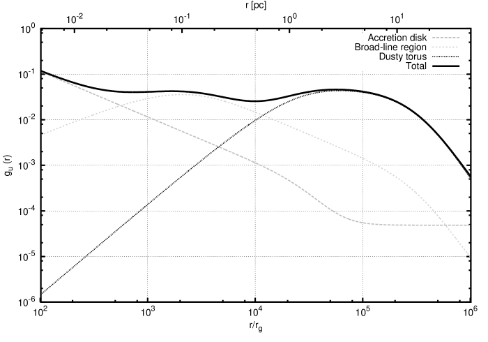
Figure 1: Geometrical correction factor $g_{u}$ as defined in Eq. A12 for external radiation planar sources: accretion disk, broad-line region and dusty torus. Parameters used in calculations: $M_{BH}=10^{9}M_{\odot}$, $\dot{M}_{d}c^{2}/L_{Edd}=10$ and $\eta_{diss}=0.5$.

References

- Abdo et al. (2010a) Abdo, A. A., Ackermann, M., Agudo, I., et al. 2010a, ApJ, 716, 30
- Abdo et al. (2010b) Abdo, A. A., Ackermann, M., Ajello, M., et al., 2010b, ApJ, 716, 835
- Ackermann et al. (2012) Ackermann, M., Ajello, M., Ballet, J., et al. 2012, ApJ, 751, 159
- Ajello et al. (2009) Ajello, M., Costamante, L., Sambruna, R. M., et al. 2009, ApJ, 699, 603
- Aleksić et al. (2011a) Aleksić, J., Antonelli, L. A., Antoranz, P., et al. 2011, A&A, 530, A4
- Aleksić et al. (2011b) Aleksić, J., Antonelli, L. A., Antoranz, P., et al. 2011, ApJ, 730, L8
- Arav et al. (1998) Arav, N., Barlow, T. A., Laor, A., Sargent, W. L. W., & Blandford, R. D. 1998, MNRAS, 297, 990
- Barnacka et al. (2013) Barnacka, A., Moderski, R., Behera, B., Brun, P., & Wagner, S. 2013, arXiv:1307.1779
- Begelman (1998) Begelman, M. C. 1998, ApJ, 493, 291
- Begelman & Sikora (1987) Begelman, M. C., & Sikora, M., 1987, ApJ, 322, 650
- Bentz et al. (2006) Bentz, M. C., Peterson, B. M., Pogge, R. W., Vestergaard, M., & Onken, C. A. 2006, ApJ, 644, 133
- Bonnoli et al. (2011) Bonnoli, G., Ghisellini, G., Foschini, L., Tavecchio, F., & Ghirlanda, G. 2011, MNRAS, 410, 368
- Celotti & Ghisellini (2008) Celotti, A. & Ghisellini, G. 2008, MNRAS, 385, 283
- Czerny & Hryniewicz (2011) Czerny, B., & Hryniewicz, K. 2011, A&A, 525, L8
- Daly & Marscher (1988) Daly, R. A., & Marscher, A. P. 1988, ApJ, 334, 539
- Dermer & Schlickeiser (2002) Dermer, C. D., & Schlickeiser, R. 2002, ApJ, 575, 667
- Elitzur (2008) Elitzur, M. 2008, New A Rev., 52, 274
- Elitzur & Shlosman (2006) Elitzur, M., & Shlosman, I. 2006, ApJ, 648, L101
- Fernandes et al. (2011) Fernandes, C. A. C., Jarvis, M. J., Rawlings, S., et al. 2011, MNRAS, 411, 1909
- Gaskell et al. (2007) Gaskell, C. M., Klimek, E. S., & Nazarova, L. S. 2007, arXiv:0711.1025
- Ghisellini & Tavecchio (2010) Ghisellini, G. & Tavecchio, F. 2010, MNRAS, 409, L79
- Ghisellini et al. (2010) Ghisellini, G., Tavecchio, F., Foschini, L., et al. 2010, MNRAS, 402, 497
- Ghisellini et al. (2011) Ghisellini, G., Tagliaferri, G., Foschini, L., et al. 2011, MNRAS, 411, 901
- Giannios & Spruit (2006) Giannios, D., & Spruit, H. C. 2006, A&A, 450, 887
- Giommi et al. (2012) Giommi, P., Polenta, G., Lähteenmäki, A., et al. 2012, A&A, 541, A160
- H.E.S.S. Collaboration (2013) H.E.S.S. Collaboration, Abramowski, A., Acero, F., et al. 2013, A&A, 554, A107
- Hayashida et al. (2012) Hayashida, M., Madejski, G. M., Nalewajko, K., et al., 2012, ApJ, 754, 114
- Horne et al. (1991) Horne, K., Welsh, W. F., & Peterson, B. M. 1991, ApJ, 367, L5
- Hoshino & Shimada (2002) Hoshino, M., & Shimada, N. 2002, ApJ, 572, 880
- Hoshino et al. (1992) Hoshino, M., Arons, J., Gallant, Y. A., & Langdon, A. B. 1992, ApJ, 390, 454
- Hönig et al. (2011) Hönig, S. F., Leipski, C., Antonucci, R., & Haas, M. 2011, ApJ, 736, 26
- Janiak et al. (2012) Janiak, M., Sikora, M., Nalewajko, K., Moderski, R., & Madejski, G. M. 2012, ApJ, 760, 129
- Kaspi et al. (2007) Kaspi, S., Brandt, W. N., Maoz, D., et al. 2007, ApJ, 659, 997
- Kataoka et al. (2008) Kataoka, J., Madejski, G., Sikora, M., et al., 2008, ApJ, 672, 787
- Kishimoto et al. (2011) Kishimoto, M., Hönig, S. F., Antonucci, R., et al. 2011, A&A, 536, A78
- Kollatschny & Zetzl (2013) Kollatschny, W., & Zetzl, M. 2013, A&A, 558, A26
- Komissarov & Falle (1997) Komissarov, S. S., & Falle, S. A. E. G. 1997, MNRAS, 288, 833
- Krolik et al. (1991) Krolik, J. H., Horne, K., Kallman, T. R., et al. 1991, ApJ, 371, 541
- Kubo et al. (1998) Kubo, H., Takahashi, T., Madejski, G., et al. 1998, ApJ, 504, 693
- Lawson & McHardy (1998) Lawson, A. J., & McHardy, I. M. 1998, MNRAS, 300, 1023
- Lovelace et al. (1997) Lovelace, R. V. E., Newman, W. I., & Romanova, M. M. 1997, ApJ, 484, 628
- Lyubarsky (2010) Lyubarsky, Y. 2010, ApJ, 725, L234
- McKinney et al. (2012) McKinney, J. C., Tchekhovskoy, A., & Blandford, R. D. 2012, MNRAS, 423, 3083
- Mor & Netzer (2012) Mor, R., & Netzer, H. 2012, MNRAS, 420, 526
- Nalewajko (2012) Nalewajko, K. 2012, MNRAS, 420, L48
- Nalewajko & Sikora (2009) Nalewajko, K., & Sikora, M. 2009, MNRAS, 392, 1205
- Nalewajko et al. (2011) Nalewajko, K., Giannios, D., Begelman, M. C., Uzdensky, D. A., & Sikora, M. 2011, MNRAS, 413, 333
- Nalewajko et al. (2012) Nalewajko, K., Sikora, M., Madejski, G. M., et al. 2012, ApJ, 760, 69
- Nenkova et al. (2008) Nenkova, M., Sirocky, M. M., Nikutta, R., Ivezić, Ž., & Elitzur, M. 2008, ApJ, 685, 160
- Peterson (1993) Peterson, B. M. 1993, PASP, 105, 247
- Poutanen & Stern (2010) Poutanen, J., & Stern, B. 2010, ApJ, 717, L118
- Punsly (2007) Punsly, B. 2007, MNRAS, 374, L10
- Rawlings & Saunders (1991) Rawlings, S., & Saunders, R. 1991, Nature, 349, 138
- Sambruna (1997) Sambruna, R. M. 1997, ApJ, 487, 536
- Sikora (2011) Sikora, M. 2011, IAU Symposium, 275, 59
- Sikora & Madejski (2000) Sikora, M., & Madejski, G. 2000, ApJ, 534, 109
- Sikora et al. (2005) Sikora, M., Begelman, M. C., Madejski, G. M., & Lasota, J.-P. 2005, ApJ, 625, 72
- Sikora et al. (2008) Sikora, M., Moderski, R., & Madejski, G. M., 2008, ApJ, 675, 71
- Sikora et al. (2009) Sikora, M., Stawarz, Ł., Moderski, R., Nalewajko, K., & Madejski, G. M. 2009, ApJ, 704, 38
- Sironi & Spitkovsky (2011) Sironi, L., & Spitkovsky, A. 2011, ApJ, 726, 75
- Spada et al. (2001) Spada, M., Ghisellini, G., Lazzati, D., & Celotti, A. 2001, MNRAS, 325, 1559
- Tanaka et al. (2011) Tanaka, Y. T., Stawarz, Ł., Thompson, D. J., et al. 2011, ApJ, 733, 19
- Tavecchio & Ghisellini (2012) Tavecchio, F., & Ghisellini, G. 2012, arXiv:1209.2291
- Vercellone et al. (2011) Vercellone, S., Striani, E., Vittorini, V., et al. 2011, ApJ, 736, L38
- Wehrle et al. (2012) Wehrle, A. E., Marscher, A. P., Jorstad, S. G., et al. 2012, ApJ, 758, 72
- Wills & Browne (1986) Wills, B. J., & Browne, I. W. A. 1986, ApJ, 302, 56